CFD Study of the Impact of Variable Cant Angle Winglets on Total Drag Reduction


DICCA, Università degli Studi di Genova, Via Montallegro 1, 16145 Genova, Italy
*
Author to whom correspondence should be addressed.
Aerospace 2018, 5(4), 126; https://doi.org/10.3390/aerospace5040126
Submission received: 24 September 2018
/
Revised: 24 November 2018
/
Accepted: 26 November 2018
/
Published: 3 December 2018
(This article belongs to the Special Issue Bio-Inspired Aerospace System)
Abstract
:Winglets are commonly used drag-reduction and fuel-saving technologies in today’s aviation. The primary purpose of the winglets is to reduce the lift-induced drag, therefore improving fuel efficiency and aircraft performance. Traditional winglets are designed as fixed devices attached at the tips of the wings. However, because they are fixed surfaces, they give their best lift-induced drag reduction at a single design point. In this work, we propose the use of variable cant angle winglets which could potentially allow aircraft to get the best all-around performance (in terms of lift-induced drag reduction), at different angle-of-attack values. By using computational fluid dynamics, we study the influence of the winglet cant angle and sweep angle in the performance of a benchmark wing at a Mach number of 0.8395. The results obtained demonstrate that by carefully adjusting the cant angle, the aerodynamic performance can be improved at different angles of attack.
1. Introduction
Aircraft winglets are small wing extensions attached at the wingtips, which are angled upward or downward (but operational requirements and ground clearances favor winglets bent upwards). They can also bend smoothly up like birds’ wingtip feathers in flight. In Figure 1, it can be seen how the wingtip feathers of different birds are bent up and separated (like the fingers of a spreading hand). This wingtip feather slotted configuration is thought to reduce the lift-induced drag caused by wingtip vortices. Tucker [1] showed that the presence or absence of these tip slots has a significant effect on the drag of birds. He found that the drag of a Harris hawk gliding freely at equilibrium in a wind tunnel increased markedly when the tip slots were removed by clipping the primary feathers. The slots also appear to reduce drag by vertical vortex spreading, because the greater wingspan and other differences in the bird with intact tip slots did not entirely account for its lower drag.
During the 1970s oil crisis, commercial airlines and aircraft manufacturers explored many ways to reduce fuel consumption because of the high cost of jet fuel. It was not until the late 1970s that R.T. Whitcomb, an engineer at NASA Langley Research Center, further developed the concept of winglets and pioneered the design of the modern winglet as a mean to reduce cruise drag and improve aircraft performance [2]. Whitcomb was inspired by an article in Science Magazine on the flight characteristics of soaring birds and their use of tip feathers to control flight. Whitcomb designed a winglet using advanced airfoil concepts integrated into a swept, tapered planform that would interact with the wingtip airflow to reduce drag.
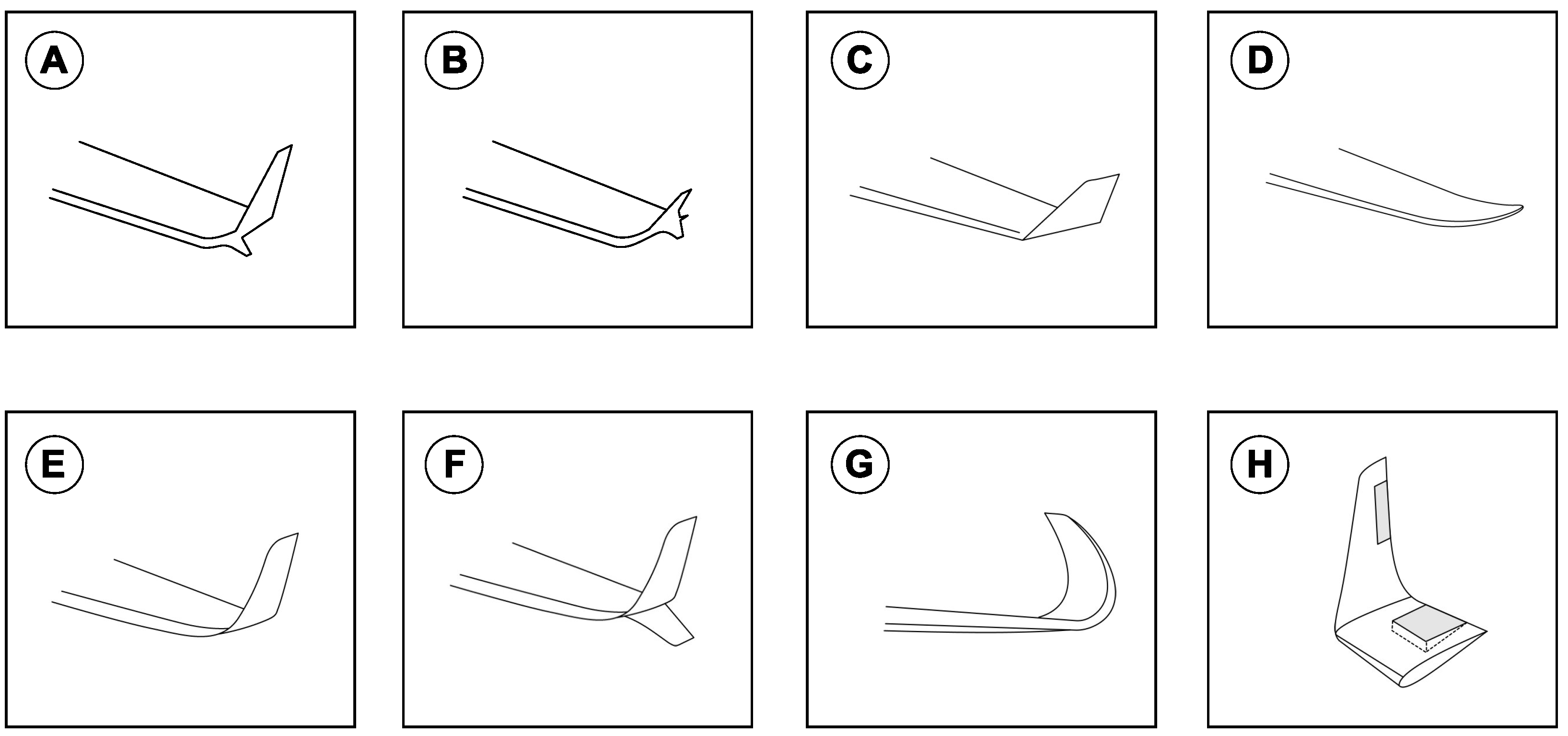
Whitcomb’s work [3], marks the first time a winglet was seriously considered for large and heavy aircraft. Since Whitcomb breakthrough work on winglets, many variations have been designed (as depicted in Figure 2), but all of them have been designed as passive or fixed devices attached at the wingtips. That is, the angle between the wing plane and the winglet plane (or cant angle) does not change; therefore, they are designed to give the best lift-induced drag reduction at one design point and depending on the aircraft mission, they are usually optimized for a given flight condition (e.g., in medium- and long-range aircraft, cruise conditions, where they operate most of the times).
Hereafter, we study the use of variable cant angle winglets for drag reduction. The proposed adaptive winglet resembles the up-curved wingtip feathers of birds that contributes to enhancing flight efficiency in birds, as demonstrated by Tucker [1]. However, contrary to natural fliers, where the wingtip feathers are slotted and they bend in response to the forces experienced on them, in the proposed device, we use a single surface and the bending is achieved mechanically.
In the suggested winglet configuration, the cant angle can be changed from a planar configuration up to a vertical layout (including intermediate cant angles) and vice-versa. Therefore, the winglet can be adjusted at different flight conditions to get the best lift-induced drag reduction for the given flight phase. Similar solutions have been already proposed, but most of them focused on the use of shape memory alloy materials [4,5,6,7], foldable wings during ground operations [8,9,10,11], and complaint surfaces [12,13,14,15]; but just a few of them have addressed variable cant angle winglets for drag reduction while flying [16,17,18,19].
The concept presented hereafter represents an innovative approach that the authors’ hope holds potential to realize the goal of improving aircraft efficiency by reducing fuel consumption, cutting carbon dioxide and nitrogen oxide emissions, and lowering the perceived external noise; as drafted in the reports ACARE Vision 2020 [20] and ACARE Flight Path 2050 [21].
2. A Brief Review of Lift-Induced Drag and Its Reduction Using Winglets
Finite span wings generate lift due to the pressure imbalance between the bottom surface (high pressure) and the top surface (low pressure), as illustrated in Figure 3A. As a consequence of this pressure differential, cross flow components of velocity are generated. The higher-pressure air under the wing flows around the wingtips and tries to displace the lower pressure air on the top of the wing. This motion generates a trailing edge vortex (as illustrated in Figure 3A, and at the tips, where the flow curls, it generates large vortices, as sketched in Figure 3B. These structures are referred to as wingtip vortices and high velocities and low pressure exist at their cores. These vortices (the trailing edge vortex and wingtip vortices), produce a downward flow in the neighborhood of the wing, known as the downwash and is denoted with the letter w in Figure 4A. The downwash interacts with the free-stream velocity to induce a local relative wind deflected downward in the vicinity of each airfoil section of the wing. The presence of the downwash reduces the angle-of-attack that each section of the wing effectively sees, and it creates a component of drag, the lift-induced drag.
In Figure 4A, the angle between the airfoil chord line and the direction of the undisturbed free-stream is the angle-of-attack (AOA), which we will call geometric AOA. In this figure, the local relative wind is inclined downward due to the downwash w, which gives rise to the induced angle-of-attack or . Therefore, the angle-of-attack actually seen by the local airfoil section is the angle between the chord line and the local relative wind, or the effective angle-of-attack defined as . Even if the wind is at a geometric AOA, the local airfoil section always sees a smaller angle. This variation of the local AOA is more pronounced towards the wingtips, where the downwash is stronger. As depicted in Figure 4A, in the presence of the downwash, the local lift vector is inclined by the angle . As it can be seen in this figure, there is a component of the local lift vector in the direction of the undisturbed free-stream; that is, the presence of the downwash creates drag. This drag is what we call lift-induced drag and is an unavoidable consequence of lift generation in finite span wings.
A scenario similar to the downwash of the wing can be found at the winglets. Consider a section of the winglet as illustrated in Figure 4B. At the winglets, the tip vortex is rolling up, therefore is generating a sidewash which induces a velocity component pointing towards the fuselage. As for the wings, the induced velocity component will create a local relative wind that will tilt the local lift vector, and for well-designed winglets the force component parallel to the undisturbed free-stream will point forward, therefore generating thrust (in analogy to sails in a sailboat). Consequently, the thrust generated by the winglet counteracts any skin friction and interference drag generated by the winglet.
Well-designed winglets will reduce the trailing vortex strength and the average wing downwash, therefore, the intensity of the wingtip vortex, by modifying the pressure distribution (which is related to the spanwise lift distribution) and shifting the shed vorticity away from the wing plane. They will also counteract the skin friction and interference drag of the winglets by generating a thrust force induced by the sidewash [3,22]. All this translates into less total drag due to the reduction of lift-induced drag and the parasite drag generated by the winglet.
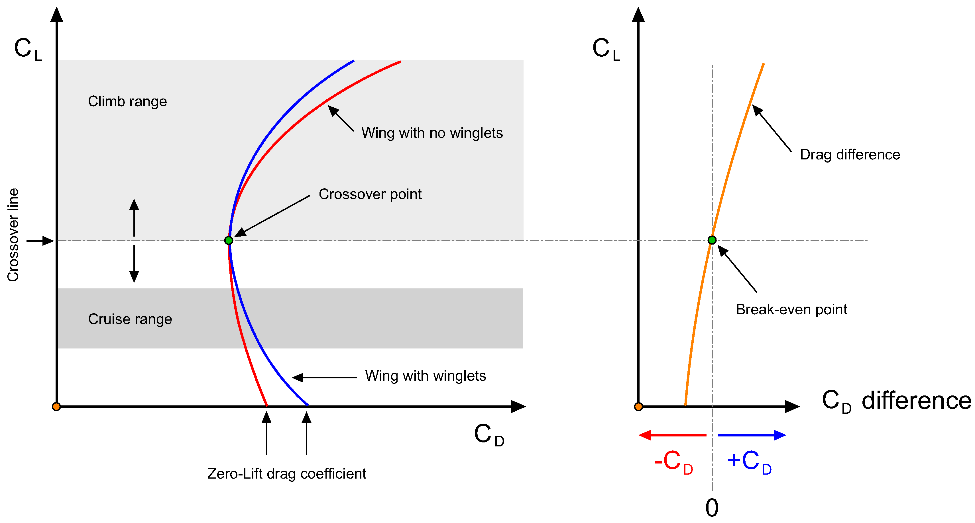
Winglets do not all look the same (as illustrated in Figure 2); nevertheless, their ultimate goal is always lift-induced drag reduction. However, winglets also increase parasite drag; hence, winglets are aerodynamically viable only when the reduction of lift-induced drag is larger than the increment in parasite drag, and this situation is illustrated in Figure 5. In this figure, we show the drag polars of two hypothetical wings, one wing with no winglets and one wing with winglets installed. In this figure, we can evidence that when operating above the crossover line or the line that passes through the crossover point (which is the point where the two polars intersect), the total drag of the wing with winglets is lower than the total drag of the wing with no winglets. Conversely, when operating below the crossover line, the total drag of the wing with no winglets is lower than the total drag of the wing with winglets. Therefore, to justify the use of winglets in the hypothetical situation illustrated in this figure, we should look at the performance of the wing at a given flight condition. Thus, if the wing were to operate most of the time in climb conditions (the light grey region in Figure 5), the use of winglets is justified because the wing with winglets generates less drag for the same lift coefficient. On the other hand, if the wing were to operate in cruise conditions in an ordinary basis (the dark grey region in Figure 5), the use of winglets is not justified as more drag is generated for the same lift coefficient.
To follow up from the previous discussion, the justification of the use of winglets can be based on the location of the crossover point in the drag polar. Therefore, the lower the crossover point location in the vertical axis is, the more desirable the use of winglets is.
3. Wing Model, Computational Domain, Boundary Conditions, and Initial Conditions
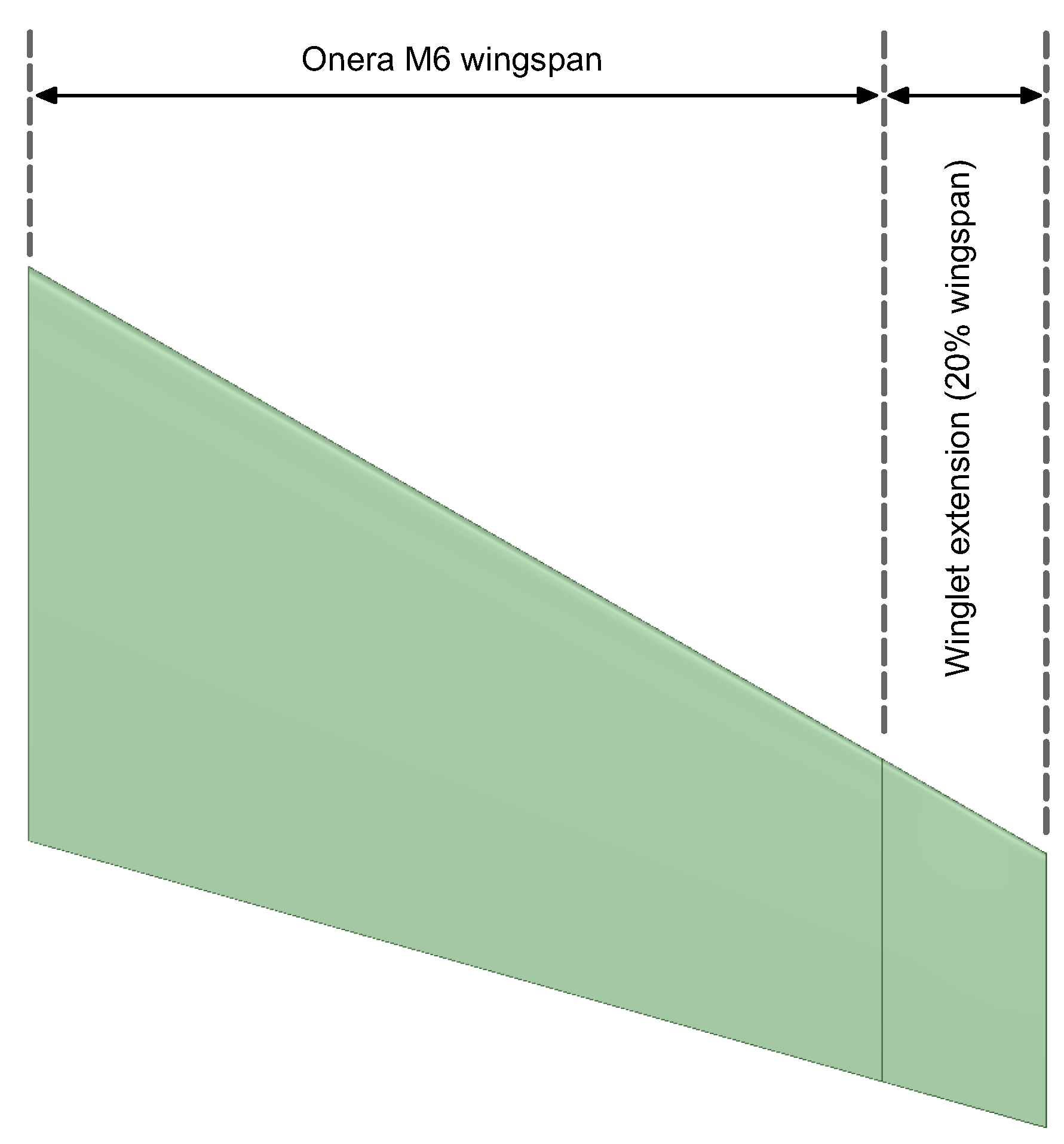
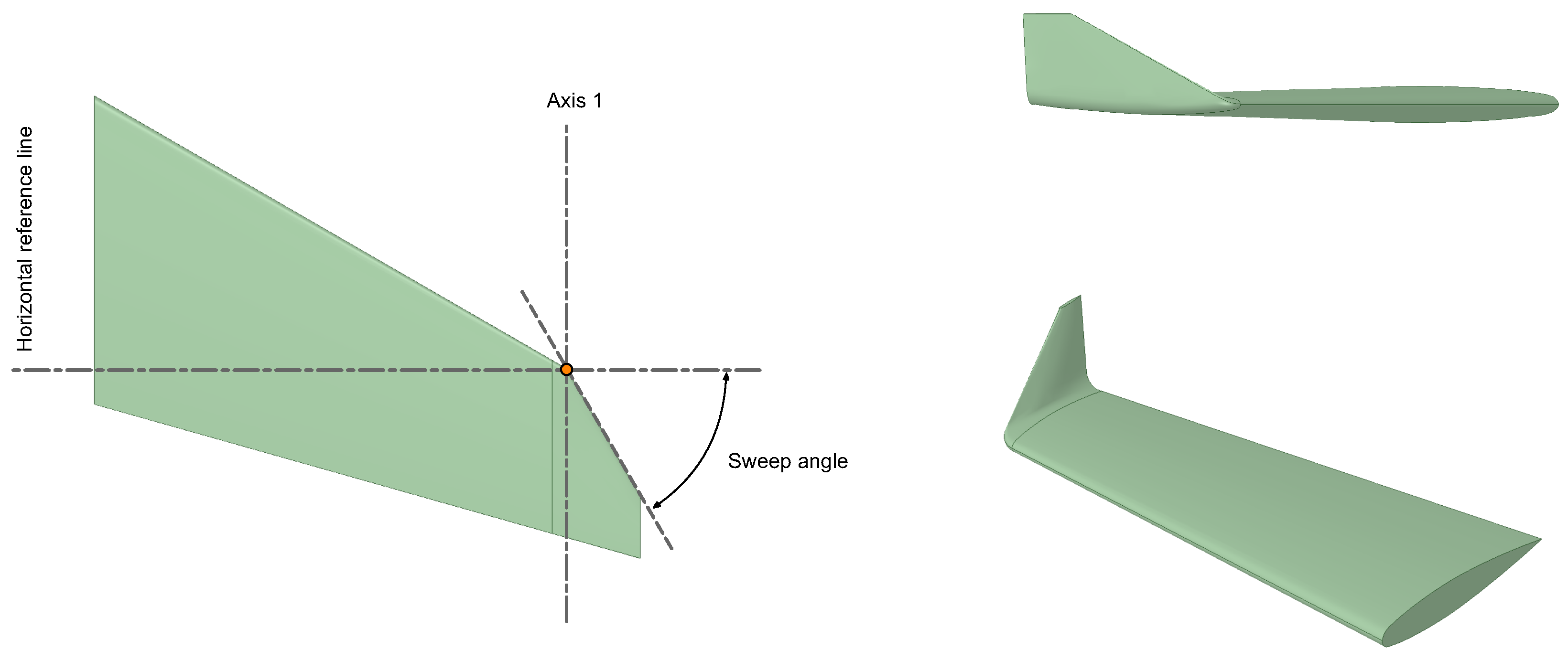
The wing model used in this study is the Onera M6, as described in references [23,24]. To model the variable cant angle winglet, an extension to the baseline Onera M6 wing was added (as shown in Figure 6). Then, the cant angle is modeled by adding a small curvature radius at the wingtip join with the winglet, in such a way as to guarantee a smooth transition between the wing and the winglet (as illustrated in Figure 7). The winglet span used in this study corresponds to a 20% of the wingspan of the baseline wing. This value was chosen based on previous studies conducted by different authors [3,25,26], where they suggest the use of winglet’s span values between 10% and 20% of the wingspan. Additionally, we also studied the influence of the winglet’s sweep angle on the aerodynamic performance of the wing. The sweep angle of the winglet is defined as illustrated in Figure 8. In Table 1 we report the cant angles, sweep angles, and angle-of-attack values used in this study. For completeness, in Table 2 we show the wetted area of each wing used hereafter.
In Figure 9, a sketch of the computational domain and the boundary conditions layout is shown. The far-field boundary in this figure corresponds to a Dirichlet type boundary condition and the outflow to a Neumann type boundary condition. The boundaries were placed far enough of the wing surface so there are no significant gradients normal to the surface boundaries. The wing was modeled as a no-slip wall, where we used continuous wall function boundary conditions for the turbulence variables. In all cases, the average distance from the wing surface to the first cell center off the surface is approximately four viscous wall units ( ). A hybrid mesh was used for all the simulations, with prismatic cells close to the wing surface and tetrahedral cells for the rest of the domain. A typical mesh is made up of approximately 3.6 to 4.1 million cells, depending on the winglet’s cant and sweep angle.
The lift force L and drag force D are calculated by integrating the pressure and wall-shear stresses over the wing surface; then, the lift coefficient and drag coefficient are computed as follows:
where is the air density (measured in ), the free-stream velocity (measured in m/s), and is the wing reference area (measured in m). During this study, air thermophysical properties were computed for air at sea-level and K.
During the parametric study, the AOA was changed by adjusting the incidence angle value of the inlet velocity and all forces were computed in the reference system aligned with the inlet velocity. All the computations were initialized using free-stream values and the incoming flow is characterized by a turbulence intensity value equal to 5.0%. All the turbulence variables were initialized following the guidelines given in references [27,28].
4. Numerical Method and Validation
The compressible Reynolds-Averaged Navier-Stokes (RANS) equations are solved by using the finite volume solver Ansys Fluent [29]. The cell-centered values of the variables are interpolated at the face locations using a second-order centered difference scheme for the diffusive terms. The convective terms at cell faces are interpolated by means of a second-order upwind scheme. For computing the gradients at cell-centers, the least squares cell-based reconstruction method is used. To prevent spurious oscillations, a multi-dimensional gradient limiter is used. The pressure-velocity coupling is achieved by means of the SIMPLE algorithm, where we used the default under-relaxation parameters. As the solution takes place in collocated meshes, the Rhie-Chow interpolation scheme is used to prevent the pressure checkerboard instability. For turbulence modeling, the SST model is used [27,28]. The turbulence quantities, namely, turbulent kinetic energy and specific dissipation rate , are discretized using the same scheme as for the convective terms. In this study, the air was modeled as an ideal gas, and we used the two coefficients Sutherland equation to compute the dynamic viscosity.
Before proceeding to the parametric study, we assessed the accuracy of the numerical scheme and mesh resolution used. In this validation study, we compared the numerical solution outcome against the data of the physical experiments at the same operating conditions described in the report [23], that is, Reynolds number equal to , Mach number equal to 0.8395, and angle-of-attack equal to .
In Figure 10, we plot the pressure coefficient values obtained from the numerical simulations against the experimental values at different wingspan locations, where is computed as follows,
in this equation, p is the pressure (measured in Pascal), and the subscript ∞ indicates the free-stream values. As it can be seen in Figure 10, the numerical solution shows a similar trend to the distribution obtained in the wind tunnel experiments. Additionally, in Table 3 we compare the and values obtained in the current study against the values obtained using different CFD solvers [24]. In this validation study, the reference area used for and computations is equal to 0.7532 m (as reported in reference [23]). In this table, we can evidence a good match among all solvers, even if the meshes and solution methods are different. Based on these results, we can state that the selected numerical scheme, turbulence model, and mesh resolution are adequate to resolve the physics involved.
As a side note, the turbulence model used in reference [24] was the Spalart-Allmaras whereas in this study we used the SST. Also, we did not model the rounded wingtip as described in references [23,24]. These two factors represent a source of uncertainty that might have affected the results presented in Table 3, which however we deem to be negligible for the purposes of this study.
5. Results and Discussion
Hereafter, we discuss the results of the aerodynamic performance of the wing with a variable cant angle winglet in reference to the baseline wing (original Onera M6 wing). To gather the data, an extensive campaign of simulations was carried out, as per the design space listed in Table 1. In this parametrical study, the reference area used for and computations is equal to 1.0 m. The computations were carried out in parallel using twelve processors, and each simulation took approximately 4 to 6 h. In this section, we discuss the results at Mach number equal to 0.8395, which might correspond to a typical velocity encountered at cruise conditions on medium- and long-range subsonic civil transport aircraft [30,31].
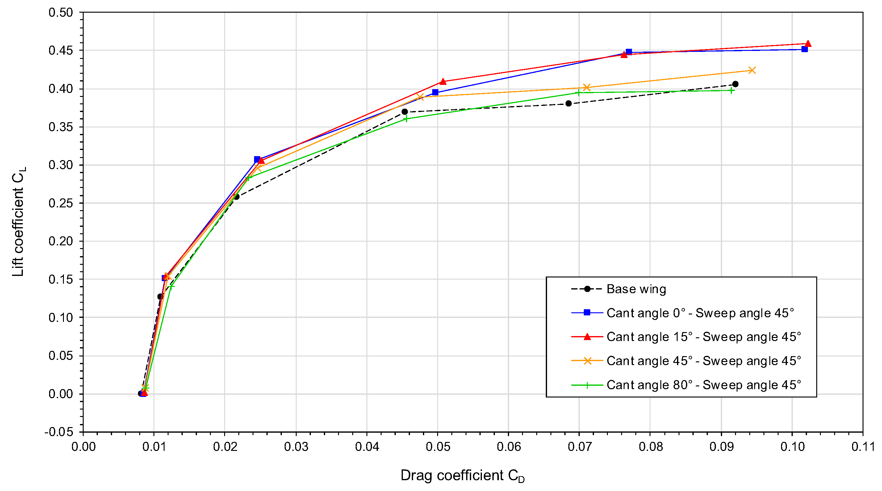
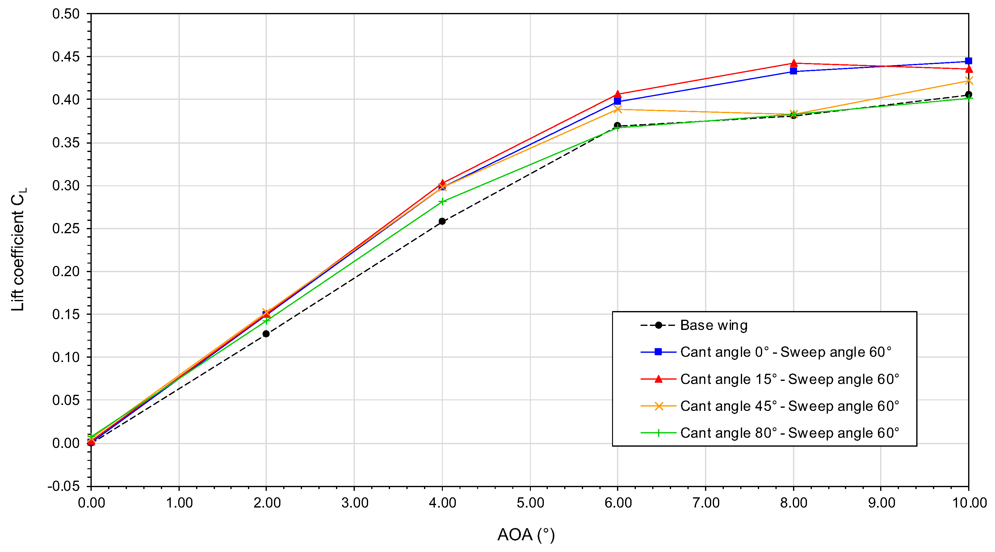
Let us now use the drag polars plotted in Figure 11, Figure 12 and Figure 13 to study the influence of the winglet cant angle and sweep angle on the aerodynamic performance of the wing. By looking at these figures, we can notice the influence of the sweep angle on the drag polars, that is, as we increase the sweep angle, the drag polar curves are shifted upwards and this trend contributes to an improvement of the aerodynamic performance, i.e., for the same lift coefficient less drag is produced.
To better highlight the influence of the sweep angle on the aerodynamic performance, in Figure 14 we plot the drag polars for fixed cant angles and different sweep angles. From this figure, it is clear that as we increase the sweep angle the crossover point is shifted downwards, up to the point that the performance of the wing with winglets is better in the whole envelope of the drag polar. Particular attention should be pay to the case with a cant angle equal to , where for sweep angle of the crossover point is located approximately at of AOA.
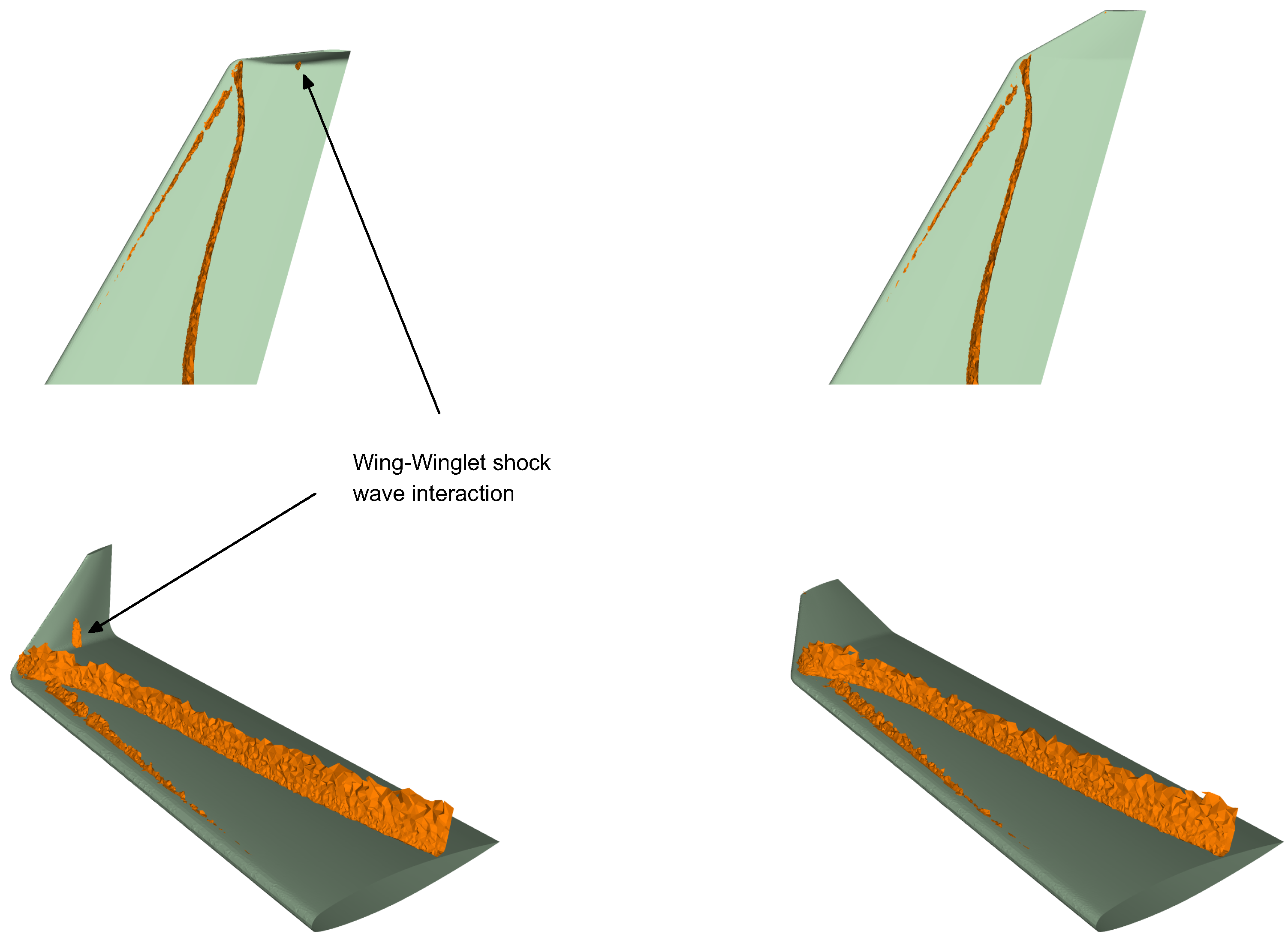
The effect of the winglet sweep angle on the aerodynamic performance can be explained by the fact that at higher sweep angles less parasite drag is produced. Another factor that contributes to the drag reduction at high Mach number, is the impact of the sweep angle on the wave drag (which we do not quantify in this study). This particular wing is known to generate a shock wave system on the wing surface; this shock wave interacts with the winglet (as depicted in Figure 15), therefore increasing the wave drag. In the figure, we illustrate the wing-winglet shock wave interaction for a winglet with a sweep angle of . For lower winglet sweep angle values ( and ), this interaction is stronger. The wing-winglet shock wave interaction might also cause boundary layer separation and buffeting. Hence, as for wings designed for high-speed, the sweep-back angle has a positive effect in reducing the wave drag in the winglets.
By quantifying the minimum drag coefficient in the drag polar plotted in Figure 11 (wing with winglet sweep angle equal to ) , we can note that the of the configuration with a cant angle of is about 30% larger than that of the base configuration, approximately 20% larger than the of the configuration with winglet cant angle equal to , and approximately 24% larger than the of the remaining winglet configurations. This trend clearly indicates that this wing-winglet design (wing with winglet sweep angle equal to ) generates a lot of parasite drag.
If we now look at Figure 12 (wing with winglet sweep angle equal to ), the situation is different, in this figure all cases generate approximately the same . However, the of the wing with a winglet at a cant angle of is approximately 2.5% larger than the of the other configurations. Finally, in Figure 13 (wing with winglet sweep angle equal to ), we observe a situation similar to the one illustrated in Figure 12, but in this case the of the wing with a winglet at a cant angle of is approximately 1.5% larger than the of the other cant angle configurations. It is also important to note that in Figure 13, none of the configurations with winglet installed have a detrimental crossover point. At low AOA (less than ), the wings with winglet generate little less drag or the difference is negligible with respect to the baseline wing. For AOA larger than the difference in for the same is more evident.
Based on these results, it was found that the winglet sweep angle has a strong influence on the aerodynamic performance of the wing and the best performance is obtained for a sweep angle equal to . Therefore, for the remainder of this section we will only discuss the results of a wing with a winglet sweep angle value equal to .
Continuing with our discussion, let us assume some hypothetical targets for the cruise and climb lift coefficients. For instance, let us say that cruise condition requires a lift coefficient close to 0.2 (which approximately corresponds to the maximum ratio [33,34]), and the maximum cruise climb lift coefficient is expected to be around 0.3 (which approximately corresponds to the maximum ratio and is on the limit of the linear regime of the lift curve). These results are shown in Table 4 and Table 5, and as it can be seen, the largest drag reduction is obtained at a cant angle value of . These results also show how the winglets reduce the drag by artificially increasing the wingspan, as it can be evidenced for cant angles equal to and .
In Figure 16, the behavior of the lift coefficient is displayed as a function of the angle-of-attack. We can observe in this figure that up to an AOA of , the lift curves display a linear behavior. We can also observe that the slope of the lift curve is almost the same for the cases with cant angle between and ( per degree). For the case with cant angle equal to the slope is lower ( per degree), but still is higher than that of the baseline wing ( per degree). Again, these results correlate well with the fact that winglets artificially increase the effective span of the wing; therefore, they have a direct impact on the lift behavior.
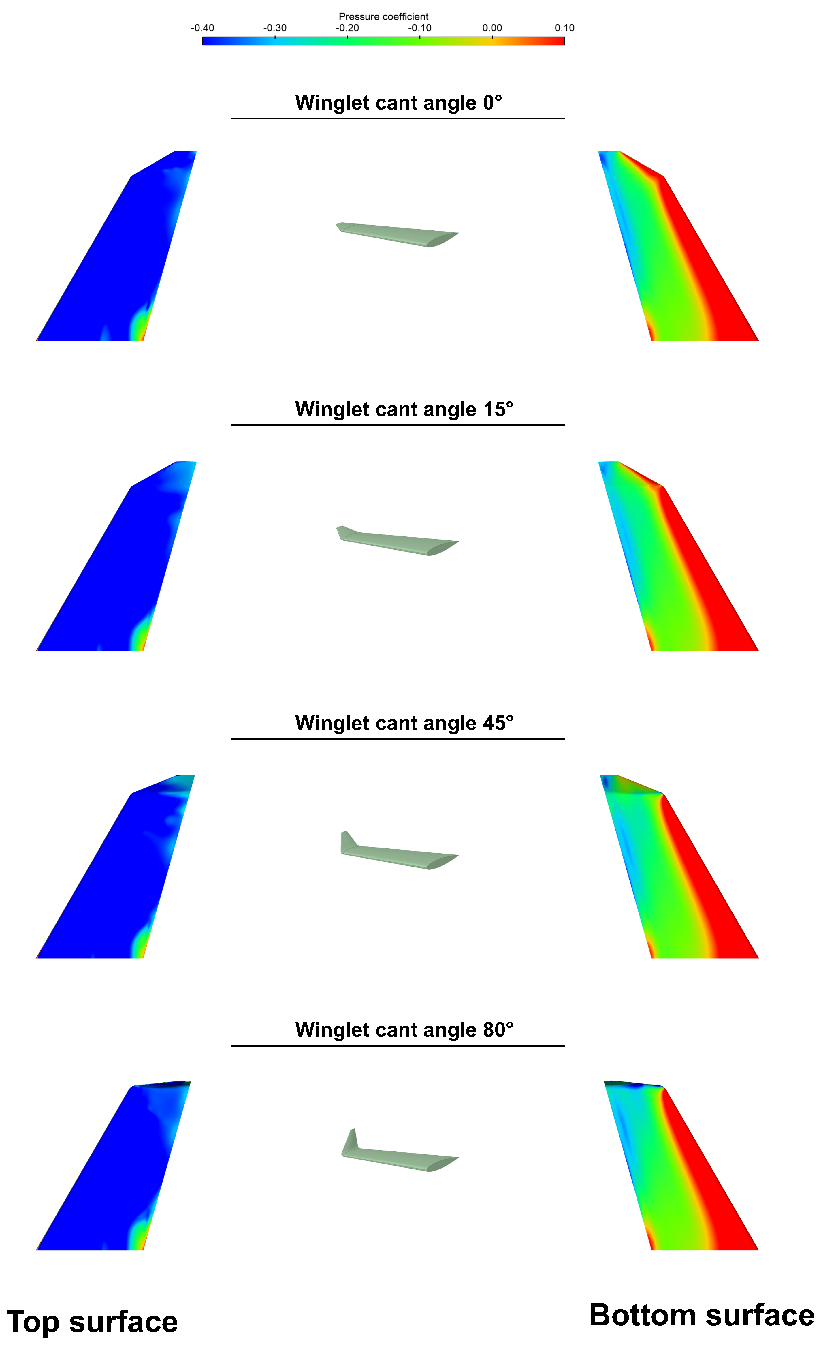
We can also observe in Figure 16 a reduction of the maximum lift coefficient for the cases with winglets at cant angle values equal to and . This decrease of the is directly related to the reduction of the pressure differential towards the wingtip as the winglet’s cant angle is increased. To understand the reason for the reduction of the pressure differential, let us look at Figure 17 where the pressure coefficient on the wing surface is displayed for all the winglet configurations. In this figure, we can observe that as we increase the cant angle the winglet will work as a wall that will reduce the pressure differential between the bottom and top surfaces of the wing. This reduction of the pressure differential, which is stronger towards the wingtip, is responsible for the decrement of the and the slope of the lift curve. As the cant angle is reduced, the decrement in the pressure differential is lessened, therefore increases, as it can be confirmed in Figure 16. The winglet effect of reduction of the pressure differential also affects drag. However, in this case its impact is positive, that is, the reduction of the pressure differential will diminish the drag and the intensity of the wingtip vortices. It is important to mention that computing and capturing the stall pattern in CFD is a difficult task; however, as we do not expect that the wing will operate at values close to in cruise conditions, uncertainties in the computation of can be tolerated.
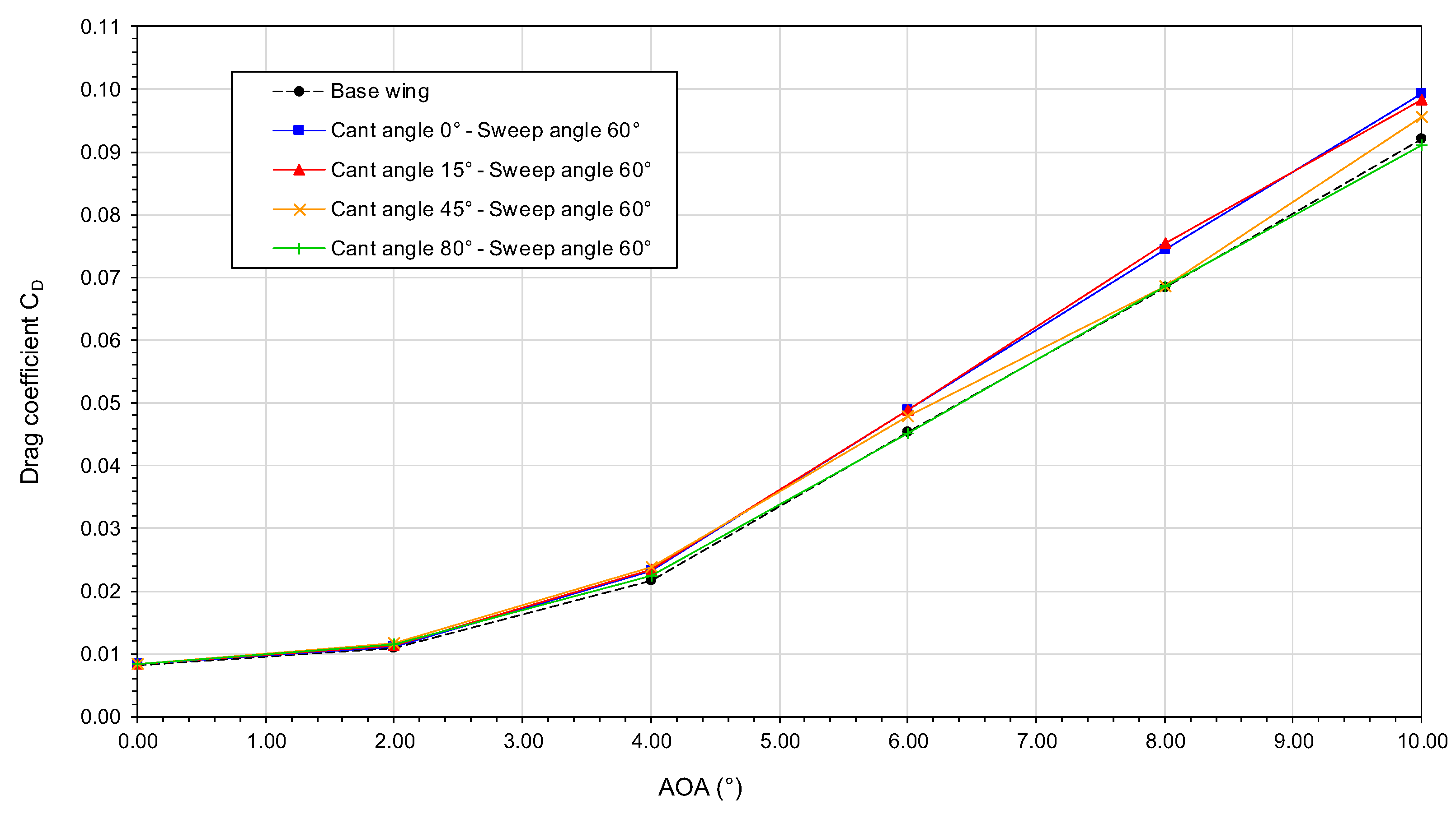
In Figure 18, we plot the behavior of the drag coefficient as a function of the angle-of-attack. In this figure, we can observe that for AOA values ranging from to all the winglet configurations generate almost the same drag or less drag than the baseline wing. Then, as we pass by AOA higher cant angles ( and ) translate in less drag for the same AOA value. As the wing profile is symmetric, the minimum drag is attained at AOA , and the use of the winglet does not appear to shift the horizontal location of in Figure 18.
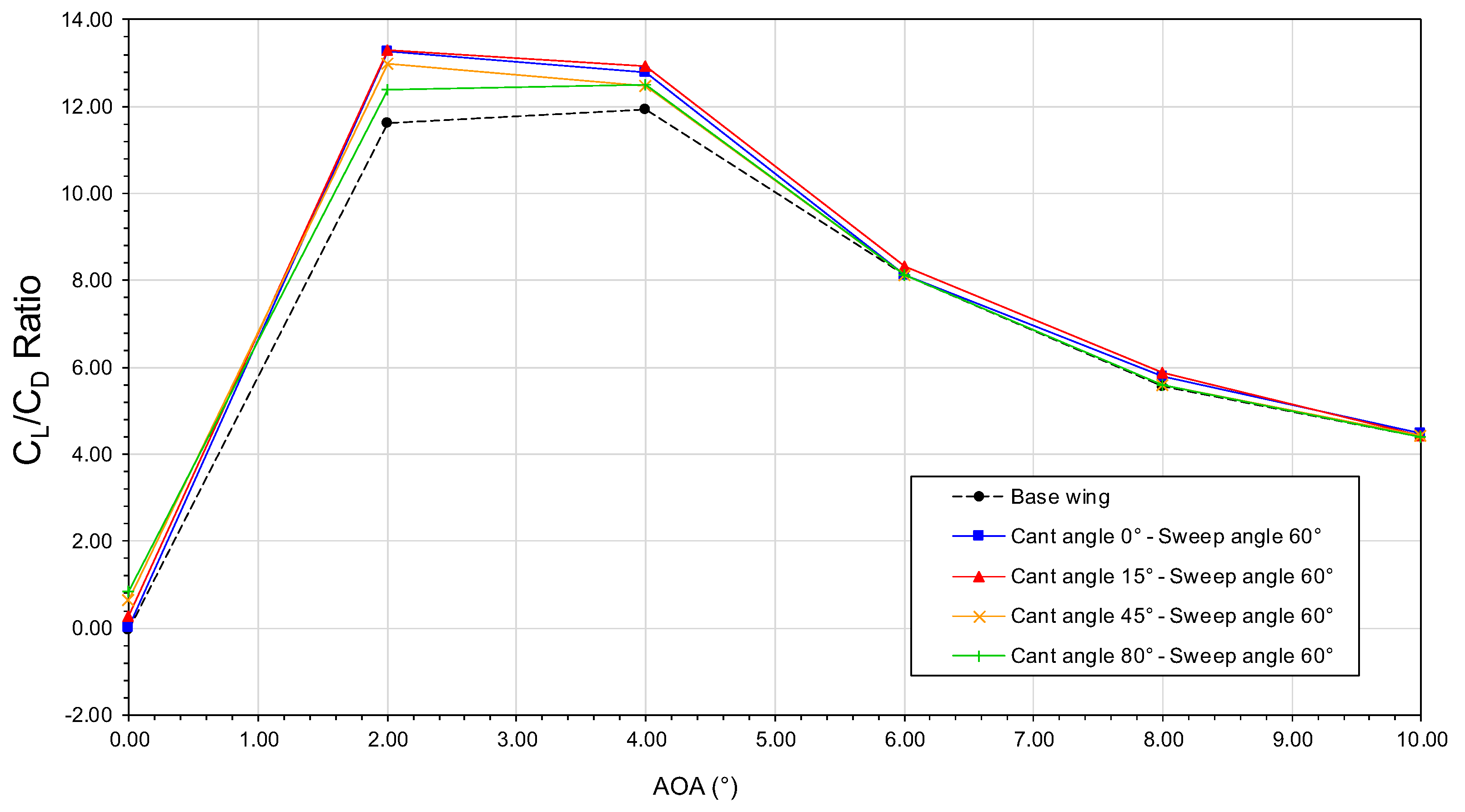
The behavior of the lift-to-drag ratio () as a function of the angle-of-attack is plotted. In Figure 19. In this figure, it is found that increases very rapidly up to about , at this point the maximum value is reached; then gradually drops mainly because drag increases more rapidly than lift. The main point of interest about the curve is the fact that this ratio is maximum at an angle-of-attack of about for all the configurations; in other words, it is at this AOA that the wings will generate as much as possible with a small production.
From the previous discussion, it is clear that there is not a single winglet configuration that can give the best all-around drag reduction at every AOA. It was also clear that the winglet configuration with a sweep angle equal to gave the best results for different cant angle values. Based on the results obtained, it is recommended to use a cant angle of at cruise conditions, which will give the largest drag reduction for a given lift. At cruise level climb, it is recommended to use a cant angle of , this selection is based on the fact that it generates fewer wing bending moments (as the slope of the lift curve is lower). In our analysis, we did not favor configurations with a cant angle value equal to due to wing-winglet shock wave interactions that might cause boundary layer separation and buffeting effects, and because they reduce the slope of the lift curve and the maximum lift coefficient. However, as it is not expected to reach in cruise conditions, the device studied might also be used as a load alleviation mechanism, where in case of strong gusts or turbulence, the cant angle can be increased to reducing in this way the slope of the lift curve, therefore decreasing the wing bending moments.
6. Conclusions and Future Perspectives
In this manuscript, we have studied the use of variable cant angle winglets which could potentially allow aircraft to get the best all-around performance in terms of drag reduction over different angle-of-attack values. While the wing studied does not correspond to an actual wing used in civil transport aircraft, the insight gathered can be used to set the guidelines for the adjustment of the winglet cant angle during flight.
All the quantitative results obtained suggest that by carefully controlling the winglet cant angle, noticeable drag reductions for the same lift value can be obtained. The proposed device can be used in cruise and cruise climb conditions, and in the case of strong gusts or turbulence, it can be used as a load alleviation mechanism. Furthermore, it was also found that large winglet sweep angle values have a positive impact on the aerodynamic performance of the wing-winglet configurations.
It is clear that to obtain the best trade-off between benefits and shortcomings, a multi-disciplinary design optimization study should be conducted, together with the use of more realistic wing geometries and additional winglet design variables, such as toe-angle, taper ratio, and span. We also envisage conducting a fight performance study using more realistic wing-winglet configurations. Nevertheless, the concept studied represents an innovative approach that might help in reducing drag, saving fuel, cutting CO and NO emissions, and lowering perceived noise. Variable cant angle winglets can also help to extend airplanes range and increase payload.
Author Contributions
Conceptualization, J.G.; Methodology, J.G.; Software, J.G., M.S. and K.W.; Validation, M.S. and K.W.; Formal Analysis, J.G., M.S. and K.W.; Investigation, J.G., M.S. and K.W.; Resources, J.G.; Data Curation, J.G., M.S. and K.W.; Writing—Original Draft Preparation, M.S. and K.W.; Writing—Review & Editing, J.G.; Visualization, J.G., M.S. and K.W.; Supervision, J.G.
Funding
This research received no external funding.
Conflicts of Interest
The authors declare no conflict of interest.
References
- Tucker, V.A. Drag reduction by wing tip slots in a gliding Harris’ hawk, Parabuteo unicinctus. J. Exp. Biol. 1995, 198, 775–781. [Google Scholar] [PubMed]
- Chambers, J.R. Concept to Reality: Contributions of the Langley Research Center to U.S. Civil Aircraft of the 1990s; NASA History Series SP-2003-4529; DIANE Publishing Company: Collingdale, PA, USA, 2003. [Google Scholar]
- Whitcomb, R.T. A Design Approach and Selected Wind Tunnel Results at High Subsonic Speeds for Wing-Tip Mounted Winglets; Technical Report NASA-TN-D-8260; NASA Langley Research Center: Hampton, VA, USA, 1976.
- Sankrithi, M.; Frommer, J. Controllable Winglets. U.S. Patent US7744038B2, 29 August 2010. [Google Scholar]
- Moholt, M.; Othmane, B. Spanwise Adaptive Wing. Presented at the 3rd Annual Convergent Aeronautics Solutions Showcase and Innovation Faire, Newport News, VA, USA, 19–20 September 2017. [Google Scholar]
- Kamlet, M. NASA Tests New Alloy to Fold Wings in Flight. Available online: https://www.nasa.gov/centers/armstrong/feature/nasa-tests-new-alloy-to-fold-wings-in-flight.html (accessed on 15 November 2018).
- Hubler, M.; Nissle, S.; Gurka, M.; Breuer, U. Fiber-reinforced polymers with integrated shape memory alloy actuation: An innovative actuation method for aerodynamics applications. CEAS Aeronaut. J. 2016, 7, 567–576. [Google Scholar] [CrossRef]
- Allen, J. Articulating Winglets. U.S. Patent US5988563A, 23 November 1999. [Google Scholar]
- Fox, S.; Kordel, J.; Townsend, K.; Lassen, M.; Gardner, M.; Good, M. Wing Fold System Rotating Latch. U.S. Patent US9469392B2, 18 October 2016. [Google Scholar]
- Axford, T.; Fong, T.; Alexander, S. An Aircraft with a Foldable Wing Tip Device. Great Britain Patent GB201407197D0, 11 August 2014. [Google Scholar]
- VIDEO: Boeing 777X Folding Wingtip. Available online: https://www.boeing.com/777x/reveal/video-777x-Folding-Wingtip/ (accessed on 15 November 2018).
- Miller, E.J.; Lokos, W.A.; Cruz, J.; Crampton, G.; Stephens, C.A.; Kota, S.; Ervin, G.; Flick, P. Approach for Structurally Clearing an Adaptive Compliant Trailing Edge Flap for Flight. In Proceedings of the 46th Society of Flight Test Engineers International Annual Symposium, Lancaster, CA, USA, 14–17 September 2015. [Google Scholar]
- Kota, S.; Osborn, R.; Ervin, G.; Maric, D. Mission Adaptive Compliant Wing—Design, Fabrication and Flight Test. In Proceedings of the RTO Applied Vehicle Technology Panel (AVT) Symposium, Evora, Portugal, 20–24 April 2009. [Google Scholar]
- Kota, S. Future Airplanes Will Fly On Twistable Wings. IEEE Spectrum, 31 August 2016. [Google Scholar]
- George, F. Aviation Partners, FlexSys to Bring Wing Morphing to Market. Available online: http://aviationweek.com/nbaa-2015/aviation-partners-flexsys-bring-wing-morphing-market (accessed on 15 November 2018).
- Barriety, B. Aircraft with Active Control of the Warping of its Wings. U.S. Patent US6827314B2, 7 December 2004. [Google Scholar]
- Bourdin, P.; Gatto, A.; Friswell, M.I. Aircraft Control via Variable Cant-Angle Winglets. J. Aircr. 2008, 45, 414–423. [Google Scholar] [CrossRef] [Green Version]
- Beechook, A.; Wang, J. Aerodynamic analysis of variable cant angle winglets for improved aircraft performance. In Proceedings of the 19th International Conference on Automation and Computing, London, UK, 13–14 September 2013. [Google Scholar]
- Panagiotou, P.; Efthymiadis, M.; Mitridis, D.; Yakinthos, K. A CFD-aided investigation of the morphing winglet concept for the performance optimization of the fixed-wing MALE UAVs. In Proceedings of the AIAA Applied Aerodynamics Conference, Atlanta, GA, USA, 25–29 June 2018. [Google Scholar]
- European Aeronautics: A Vision for 2020; Technical Report, Advisory Council for Aviation Research and Innovation in Europe; European commission: Brussels, Belgium, 2001.
- Krein, A.; Williams, G. Flightpath 2050: Europe’s vision for aeronautics. In Innovation for Sustainable Aviation in a Global Environment: Proceedings of the Sixth European Aeronautics Days; IOS Press: Amsterdam, The Netherlands, 2012; p. 63. [Google Scholar]
- Kroo, I. DRAG DUE TO LIFT: Concepts for Prediction and Reduction. Annu. Rev. Fluid Mech. 2001, 33, 587–617. [Google Scholar] [CrossRef]
- Schmitt, V.; Charpin, F. Pressure Distributions on the ONERA-M6-Wing at Transonic Mach Numbers; Technical Report AGARD Report 138; NATO: Brussels, Belgium, 1979. [Google Scholar]
- Turbulence Modeling Resource—3D ONERA M6 Wing Validation. Available online: https://turbmodels.larc.nasa.gov/onerawingnumerics_val.html (accessed on 15 November 2018).
- Shollenberger, C.A. Application of an Optimized Winglet Configuration to an Advanced Commercial Transport; Technical Report NASA-CR-159156; NASA: Washington, DC, USA, 1979.
- Smith, L.; Campbell, R. Effects of Winglets on the Drag of a Low-Aspect-Ratio Configuration; Technical Report NASA-TP-3563; NASA: Washington, DC, USA, 1996.
- Wilcox, D.C. Turbulence Modeling for CFD; DCWIndustries: La Cañada Flintridge, CA, USA, 2010. [Google Scholar]
- Menter, F.R. Two-equation eddy-viscosity turbulence models for engineering applications. AIAA J. 1994, 32, 1598–1605. [Google Scholar] [CrossRef] [Green Version]
- Ansys Academic Research, Release 19, Help System, Ansys Fluent Theory Guide; ANSYS, Inc.: Canonsburg , PA, USA, 2018.
- McCormick, B.W. Aerodynamics, Aeronautics, and Flight Mechanics; Wiley: Hoboken, NJ, USA, 1994. [Google Scholar]
- Eurocontrol—Aircraft Performance Database. Available online: https://contentzone.eurocontrol.int/aircraftperformance/ (accessed on 15 November 2018).
- Lovely, D.; Haimes, R. Shock detection from computational fluid dynamics results. In Proceedings of the AIAA 14th Computational Fluid Dynamics Conference, Norfolk, VA, USA, 1–5 November 1999. [Google Scholar]
- Raymer, D.P. Aircraft Design: A Conceptual Approach; AIAA Education Series: Reston, VA, USA, 2016. [Google Scholar]
- Sadraey, M.H. Aircraft Design: A Systems Engineering Approach; Wiley: Hoboken, NJ, USA, 2013. [Google Scholar]
Figure 1.
Birds’ wingtip feathers. (A) Great Horned Owl; (B) Swainson’s Hawk; (C) Long-Tailed Duck; (D) Bald Eagle. Images courtesy of Ad Wilson (www.naturespicsonline.com) and Rob McKay (http://robmckayphotography.com).
Figure 1.
Birds’ wingtip feathers. (A) Great Horned Owl; (B) Swainson’s Hawk; (C) Long-Tailed Duck; (D) Bald Eagle. Images courtesy of Ad Wilson (www.naturespicsonline.com) and Rob McKay (http://robmckayphotography.com).

Figure 2.
Different types of winglets and wingtip devices commonly used. (A) Whitcomb winglet; (B) Tip fence; (C) Canted winglet; (D) Raked wingtip; (E) Blended winglet; (F) Blended split winglet; (G) Sharklet; (H) Active wnglets.
Figure 2.
Different types of winglets and wingtip devices commonly used. (A) Whitcomb winglet; (B) Tip fence; (C) Canted winglet; (D) Raked wingtip; (E) Blended winglet; (F) Blended split winglet; (G) Sharklet; (H) Active wnglets.

Figure 3.
(A) Illustration of lift generation due to pressure imbalance and its associated wingtip and trailing edge vortices; (B) Illustration of wingtip vortices rotation and the associated downwash and upwash.
Figure 3.
(A) Illustration of lift generation due to pressure imbalance and its associated wingtip and trailing edge vortices; (B) Illustration of wingtip vortices rotation and the associated downwash and upwash.

Figure 4.
(A) Illustration of lift-induced drag due to downwash; (B) Illustration of forces generated at the winglets.
Figure 4.
(A) Illustration of lift-induced drag due to downwash; (B) Illustration of forces generated at the winglets.

Figure 5.
Comparison of drag polars for a clean wing and a wing with winglet installed, where is the drag coefficient and is the lift coefficient. In the left image, the light grey area represents the climb range of the wings, and the dark grey area represents the cruise range of the wings. In the right image, we show the drag difference, where negative means drag increment and positive means drag reduction. The difference is expressed as the subtraction between the wing with winglets and the wing with no winglets.

Figure 6.
Wing and winglet extension. The winglet span used in this study corresponds to a 20% of the wing span of the original Onera M6 wing.
Figure 6.
Wing and winglet extension. The winglet span used in this study corresponds to a 20% of the wing span of the original Onera M6 wing.

Figure 7.
Winglet cant angle definition (left image). The winglet extension is bent upwards about the axis 1 (right image). This axis is located 40 mm away from the wingtip. For all cases studied, the curvature radius is no more than 30 mm.
Figure 7.
Winglet cant angle definition (left image). The winglet extension is bent upwards about the axis 1 (right image). This axis is located 40 mm away from the wingtip. For all cases studied, the curvature radius is no more than 30 mm.

Figure 8.
Left image: winglet sweep angle definition. Right image: winglet geometry corresponding to a cant angle of and a sweep angle of .
Figure 8.
Left image: winglet sweep angle definition. Right image: winglet geometry corresponding to a cant angle of and a sweep angle of .

Figure 9.
Computational domain and boundary conditions (all dimensions are in meters). The illustration is not to scale.
Figure 9.
Computational domain and boundary conditions (all dimensions are in meters). The illustration is not to scale.

Figure 10.
Plot of the pressure coefficient on the wing surface at different sections. Comparison of numerical and experimental results.
Figure 10.
Plot of the pressure coefficient on the wing surface at different sections. Comparison of numerical and experimental results.

Figure 11.
Drag polar at Mach number 0.8395, winglet sweep angle and different values of cant angle.
Figure 11.
Drag polar at Mach number 0.8395, winglet sweep angle and different values of cant angle.

Figure 12.
Drag polar at Mach number 0.8395, winglet sweep angle and different values of cant angle.
Figure 12.
Drag polar at Mach number 0.8395, winglet sweep angle and different values of cant angle.

Figure 13.
Drag polar at Mach number 0.8395, winglet sweep angle and different values of cant angle.
Figure 13.
Drag polar at Mach number 0.8395, winglet sweep angle and different values of cant angle.

Figure 14.
Drag polar at Mach number 0.8395. Each image corresponds to a fix cant angle and three different values of sweep angle.
Figure 14.
Drag polar at Mach number 0.8395. Each image corresponds to a fix cant angle and three different values of sweep angle.

Figure 15.
Shock wave system for AOA and two different values of winglet’s cant angle. The shock wave region was computed using the criterion of Lovely and Haimes [32]. The left image corresponds to a winglet cant angle of and the right image to a cant angle value of .
Figure 15.
Shock wave system for AOA and two different values of winglet’s cant angle. The shock wave region was computed using the criterion of Lovely and Haimes [32]. The left image corresponds to a winglet cant angle of and the right image to a cant angle value of .

Figure 16.
Lift coefficient versus angle-of-attack at Mach number 0.8395, winglet sweep angle and different values of cant angle.
Figure 16.
Lift coefficient versus angle-of-attack at Mach number 0.8395, winglet sweep angle and different values of cant angle.

Figure 17.
Pressure coefficient on the wing surface. Winglet sweep angle equal to and wing AOA equal to .
Figure 17.
Pressure coefficient on the wing surface. Winglet sweep angle equal to and wing AOA equal to .

Figure 18.
Drag coefficient versus angle-of-attack at Mach number 0.8395, winglet sweep angle and different values of cant angle.
Figure 18.
Drag coefficient versus angle-of-attack at Mach number 0.8395, winglet sweep angle and different values of cant angle.

Figure 19.
Lift-to-drag ratio versus angle-of-attack at Mach number 0.8395, winglet sweep angle and different values of cant angle.
Figure 19.
Lift-to-drag ratio versus angle-of-attack at Mach number 0.8395, winglet sweep angle and different values of cant angle.


Table 1.
Design space explored in this study. All the angles are defined in degrees.
| Winglet cant angle | 0, 15, 45, 80 | |
| Winglet sweep angle | 30, 45, 60 | |
| Angle-of-attack | 0, 2, 4, 6, 8, 10 |
Table 2.
Wetted area of each wing used in this study.
| Wing | Wetted Area () |
|---|---|
| Baseline wing (original Onera M6 wing with no wingtip) | 1.5952 |
| Wing with winglet—Winglet sweep angle equal to | 1.7881 |
| Wing with winglet—Winglet sweep angle equal to | 1.7694 |
| Wing with winglet—Winglet sweep angle equal to | 1.7388 |
Table 3.
Comparison of and obtained with different solvers (data taken from reference [24]). The comparison is done for meshes with similar cell count.
Table 3.
Comparison of and obtained with different solvers (data taken from reference [24]). The comparison is done for meshes with similar cell count.
| Solver–Mesh Type | ||
|---|---|---|
| CFL3D–Structured mesh | 0.2661 | 0.0173 |
| USM3D–Tetrahedra + Prismatic mesh | 0.2649 | 0.0186 |
| FUN3D–Pure prismatic mesh | 0.2659 | 0.0172 |
| Current solution–Hybrid mesh (tetrahedra + prisms) | 0.2597 | 0.0188 |
Table 4.
and drag reduction percentage for a target equal to 0.2. The drag reduction percentage was computed with respect to the baseline wing (positive values indicate drag reduction).
Table 4.
and drag reduction percentage for a target equal to 0.2. The drag reduction percentage was computed with respect to the baseline wing (positive values indicate drag reduction).
| Winglet Cant Angle | Winglet Sweep Angle | Drag Reduction (%) | |
|---|---|---|---|
| 0.015359 | ≈ | ||
| 0.015220 | ≈ | ||
| 0.015706 | ≈ | ||
| 0.016007 | ≈ |
Table 5.
and drag reduction percentage for a target equal to 0.3. The drag reduction percentage was computed with respect to the baseline wing (where positive values indicate drag reduction).
Table 5.
and drag reduction percentage for a target equal to 0.3. The drag reduction percentage was computed with respect to the baseline wing (where positive values indicate drag reduction).
| Winglet Cant Angle | Winglet Sweep Angle | Drag Reduction (%) | |
|---|---|---|---|
| 0.023835 | ≈ | ||
| 0.023187 | ≈ | ||
| 0.024437 | ≈ | ||
| 0.027446 | ≈ |
© 2018 by the authors. Licensee MDPI, Basel, Switzerland. This article is an open access article distributed under the terms and conditions of the Creative Commons Attribution (CC BY) license (http://creativecommons.org/licenses/by/4.0/).
Share and Cite
MDPI and ACS Style
Guerrero, J.; Sanguineti, M.; Wittkowski, K. CFD Study of the Impact of Variable Cant Angle Winglets on Total Drag Reduction. Aerospace 2018, 5, 126. https://doi.org/10.3390/aerospace5040126
AMA Style
Guerrero J, Sanguineti M, Wittkowski K. CFD Study of the Impact of Variable Cant Angle Winglets on Total Drag Reduction. Aerospace. 2018; 5(4):126. https://doi.org/10.3390/aerospace5040126
Chicago/Turabian StyleGuerrero, Joel, Marco Sanguineti, and Kevin Wittkowski. 2018. "CFD Study of the Impact of Variable Cant Angle Winglets on Total Drag Reduction" Aerospace 5, no. 4: 126. https://doi.org/10.3390/aerospace5040126
Note that from the first issue of 2016, this journal uses article numbers instead of page numbers. See further details here.