CFD-Based Aeroelastic Sensitivity Study of a Low-Speed Flutter Demonstrator
by
Vladyslav Rozov
1,*, 
Andreas Volmering
1,
Andreas Hermanutz
2,
Mirko Hornung
2 and
Christian Breitsamter
1 1
Chair of Aerodynamics and Fluid Mechanics, Department of Mechanical Engineering, Technical University of Munich, Boltzmannstr. 15, D-85748 Garching, Germany
2
Institute of Aircraft Design, Department of Mechanical Engineering, Technical University of Munich, Boltzmannstr. 15, D-85748 Garching, Germany
*
Author to whom correspondence should be addressed.
Aerospace 2019, 6(3), 30; https://doi.org/10.3390/aerospace6030030
Submission received: 6 February 2019
/
Revised: 22 February 2019
/
Accepted: 1 March 2019
/
Published: 6 March 2019
(This article belongs to the Special Issue Aeroelasticity)
Abstract
:The goal of developing aircraft that are greener, safer and cheaper can only be maintained through significant innovations in aircraft design. An integrated multidisciplinary design approach can lead to an increase in the performance of future derivative aircraft. Advanced aerodynamics and structural design technologies can be achieved by both passive and active suppression of aeroelastic instabilities. To demonstrate the potential of this approach, the EU-funded project Flutter Free Flight Envelope Expansion for Economical Performance Improvement is developing an unmanned aerial vehicle with a high-aspect-ratio-wing and clearly defined flutter characteristics. The aircraft is used as an experimental test platform. The scope of this work is the investigation of the aeroelastic behaviour of the aircraft and the determination of its flutter limits. The modeling of unsteady aerodynamics is performed by means of the small disturbance CFD approach that provides higher fidelity compared to conventional linear-potential-theory-based methods. The CFD-based and the linear-potential-theory-based results are compared and discussed. Furthermore, the sensitivity of the flutter behaviour to the geometric level of detail of the CFD model is evaluated.
1. Introduction
The success of aircraft manufacturers depends on the continuous improvement of the efficiency and the reduction of the aircraft operating costs. These tasks can be fulfilled today by incremental enhancements. Such modifications are e.g., new materials, aerodynamic optimizations, more efficient engines, etc. [1]. On the one hand, this approach ensures that development costs are kept at a given level. On the other hand, only a limited scope for improvement is possible.
The potential of the strategy can be extended by an integrated design approach [2]. It is characterized by the fact that aeroelastic and flight control aspects are taken into account at an early design stage. This strategy may help to overcome existing limitations in incremental design refinements by expanding the design space. Hence, it leads to a further increase in the performance of the aircraft. Flexible wing technology is a promising field of application of the integrated design approach. The primary objective is to increase the efficiency of a wing without increasing its structural weight, while maintaining or even extending the flight envelope. The task can be accomplished mainly by increasing the wing span (and thus the aspect ratio) of the wing. The resulting aeroelastic challenges are addressed by aeroelastic tailoring and active load control.
The potential of the integrated design approach is demonstrated within the EU-funded project Flutter Free FLight Envelope eXpansion for ecOnomical Performance improvement (FLEXOP). One of the main objectives is to design and build a cost-effective experimental test platform with a high-aspect-ratio-wing. Novel multidisciplinary methods and tools for aeroelastic design and active control are developed and validated on three different wing configurations with clearly defined structural and aeroelastic properties. Active flutter control methods are tested on the “flutter” wing. In order to ensure a cost-efficient realization of the test articles, the wing was designed in such a way that it has both a low flutter speed and a low flutter frequency of flutter-critical structural modes. Due to the strict design limitations, methods for exact flutter prediction are particularly important throughout the entire development process.
To reduce uncertainties regarding the flutter limit, this work uses a small disturbance CFD (SD-CFD) method for modelling the unsteady aerodynamics. The method is based on the full set of Euler equations. Therefore, in contrast to linear-potential-theory-based methods, it offers better accuracy with respect to complex three-dimensional flows as well as thickness and compressibility effects [3]. The technique was first developed for turbomachinery applications [4] and later extended to external aerodynamics.
The applicability of SD-CFD technique to subsonic, transonic and supersonic inviscid external flow problems was shown in e.g., [5]. The extension of the methodology towards viscous flows was demonstrated in [6,7,8,9].
Various researchers have shown that the method can be employed to several realistic engineering problems. The applications range from the calculation of dynamic stability derivatives [10,11] to aero-servo-elastic investigations [12] to the generation of reduced order models [13]. However, in the context of this work the method is used for the CFD-based computation of the generalized aerodynamic forces for use in conventional linear flutter analysis.
In this work, the aeroelastic behaviour of the FLEXOP model is investigated. Thereby, the SD-CFD results are compared to the results generated by the doublet lattice method (DLM). DLM is a potential-theory-based method that found widespread application in industrial aircraft design. Its developement is outlined in [14,15,16]. In addition, the sensitivity of the flutter limit to the geometric level of detail of the aerodynamic model is evaluated. Therefore, the influence of the actuator fairing mounted under the wing on the flutter limit is analysed.
2. Theory and Numerical Methods
In the following, the CFD-based methodology for aeroelastic analysis is presented. The equations of aeroelasticity and the SD-Euler equations are discussed. Moreover, the concept of generalized aerodynamic forces (GAF) is introduced in the context of flutter analyses.
2.1. Equations of Aeroelasticity
Starting point for a CFD-based aeroelastic analysis is a system of equations that describes the dynamics of a structural system under the influence of external unsteady forces . These equations are typically formulated in terms of physical coordinates, i.e., displacements and rotations. It is convenient to reduce the order of the system by transferring it to generalized coordinates. Thus, the equations of motion can be written as follows
is the modal matrix comprising N mode shapes . It defines the transformation between the physical and the generalized coordinates:
The diagonal matrices and contain generalized mass, damping and stiffness for each modal coordinate. The vector of generalized aerodynamic forces is computed by means of CFD simulations within this work. Dynamic pressure and the cube of the grid reference length arise in Equation (1) due to a nondimensional formulation of the CFD code. Pressure-induced aerodynamic forces acting on each mode i can be computed as follows:
The vector represents a chunk of describing the local deflection of mode i. It can be seen that the contribution of the pressure-induced load to the generalized aerodynamic force is weighted by the scalar product of the local modal deflection and the surface normal vector .
In accordance with the classical aeroelastic stability analysis, sufficiently small structural deflections are considered in the context of this work. Hence, the relation between structural deflections and unsteady aerodynamic forces is linear. It follows that the aerodynamic response to a transient structural excitation can be described employing the principle of superposition [17]. Therefore, generalized aerodynamic forces are computed by means of the convolution integral
where denotes the impulse response matrix formulated in terms of generalized coordinates. However, the frequency domain formulation of Equation (1) is used within this work. It is the well-established flutter equation, which can be written as:
In this context, is the angular velocity and is a dimensionless frequency parameter usually defined in terms of the semi-chord and freestream velocity :
The transfer matrix of generalized forces is denoted by . Each complex element can be used to evaluate the magnitude and phase of the force acting on the modal coordinate i due to a harmonic motion of the generalized coordinate j with a unit amplitude at a frequency .
2.2. Modelling of Unsteady Aerodynamics by Means of SD CFD Methodology
This section recapitulates the SD CFD methodology that is employed for unsteady aerodynamics modelling in this work. The relevant equations and aspects of the Euler solver AER-Eu and the SD-Euler solver AER-SDEu are also discussed.
SD CFD methods can be derived either from the Euler or the Navier-Stokes equations by assuming a sufficiently small, harmonic disturbance of the flow quantities around a reference state. The formulation in the frequency domain eliminates the time dependence of the problem. The consequence is a one order of magnitude faster analysis of unsteady aerodynamics compared to time-accurate CFD simulations [5]. The flow governing equations are solved directly for the complex first harmonic of the disturbed flow.
The SD-Euler solver AER-SDEu developed in [5] at the Chair of Aerodynamics and Fluid Mechanics of the Technical University of Munich is used here. It is based on the solver AER-Eu that computes nonlinear Euler equations formulated in terms of curvilinear coordinates , , :
The equations describe the conservation of mass, momentum, and energy. The vector Q is composed of conservative flow variables and F, G and H define the convective fluxes of Q in -, -, -direction. The equations are discretized by means of the finite volume (FV) method. The SD Euler equations can be derived from the nonlinear Euler equations by introducing small harmonic oscillations of the flow variables and the geometrical metrics of the computational grid around a reference state. Given a variable defining a flow quantity or a geometrical metric , the oscillation can be expressed as:
whereas the bar denotes the reference state variable and the hat denotes the disturbance amplitude that is complex-valued for flow quantities and real-valued for geometrical metrics. A linearization of Equation (7) using small disturbance assumptions defined by Equation (8) yields a set of linear PDEs [5]:
The system of equations is solved for the vector of disturbance parts of the flow variables . The superscript refers to terms determined by the disturbance components of the flow variables and the reference grid metric. The superscript denotes inhomogeneous terms that depend on the reference flow state and the disturbance components of the grid metric. Based on the known reference state of the flow and the given movement of the grid, the -terms are calculated prior to the iterative solution process. The difference between the reference grid and the deformed grid is used to determine the disturbance components of the grid metric. Therefore, both grids are required as inputs to the SD solver. Due to the dependence of Equation (9) from , the solution of the SD equations must be performed for each reduced frequency of interest. Nevertheless, as mentioned above, the SD equations can be solved more efficiently than the time-accurate nonlinear Euler equations due to their linear nature and the absence of time dependency. Numerical aspects regarding the solvers AER-Eu and AER-SDEu can be found in [5].
Once a SD solution is computed for a certain reduced frequency , unsteady aerodynamic loads harmonically acting with upon the structure are known. Subsequently, the matrix can be evaluated directly as follows for an entry [18]:
where denotes the reference state of the vector surface element. Moreover, refers to the disturbance of the vector surface element due to modal deflection of mode j.
3. The Flutter Suppression Demonstrator FLEXOP
3.1. UAV Configuration
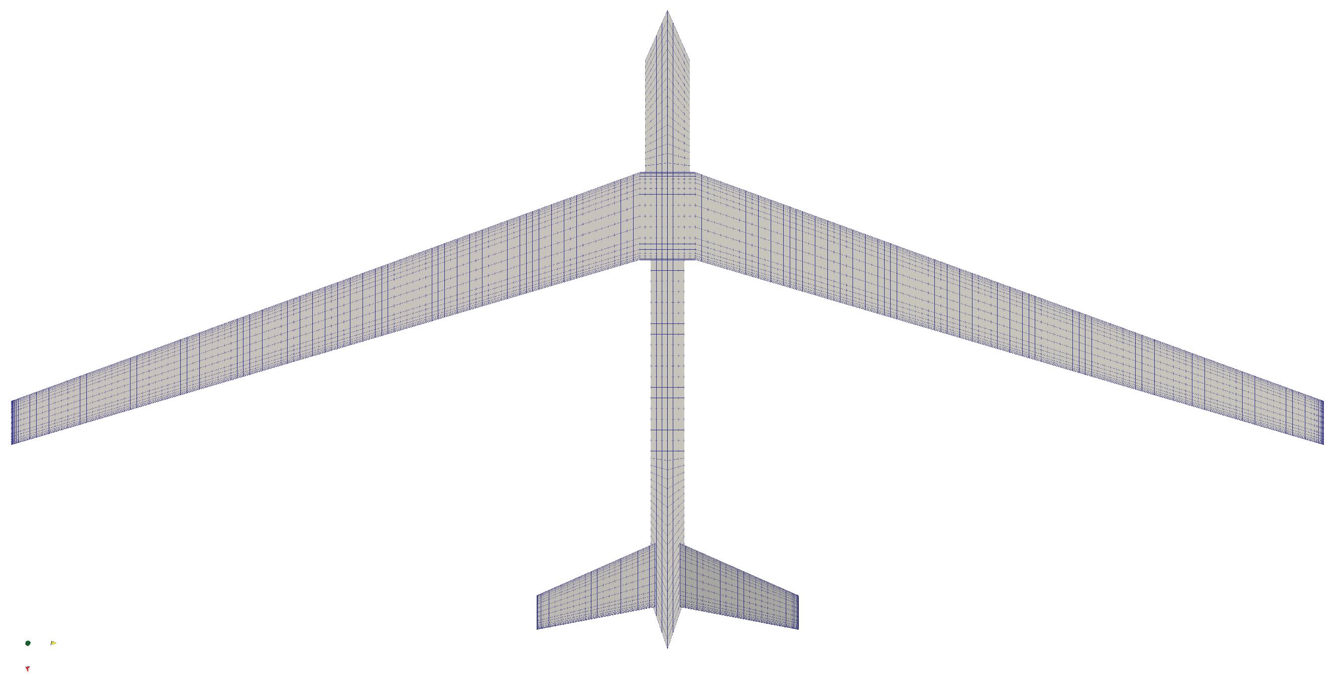
The total takeoff weight of the aircraft including all its components and fuel is 65 kg. The wing with a leading edge sweep of has a high aspect ratio of , a span of m and a reference area of m. The mean aerodynamic chord (MAC) is m and the length of the fuselage is m. The planform geometry of the FLEXOP UAV is depicted in Figure 1, where the actuator positions are indicated in blue.
Due to its modular design, the FLEXOP UAV can be equipped with three different wing configurations with clearly predefined aeroelastic properties. The tail control surfaces are arranged in a V-tail configuration. A turbojet engine mounted on top of the fuselage provides thrust. In contrast to the inertia of the engine, its aerodynamic influence is neglected in this study.
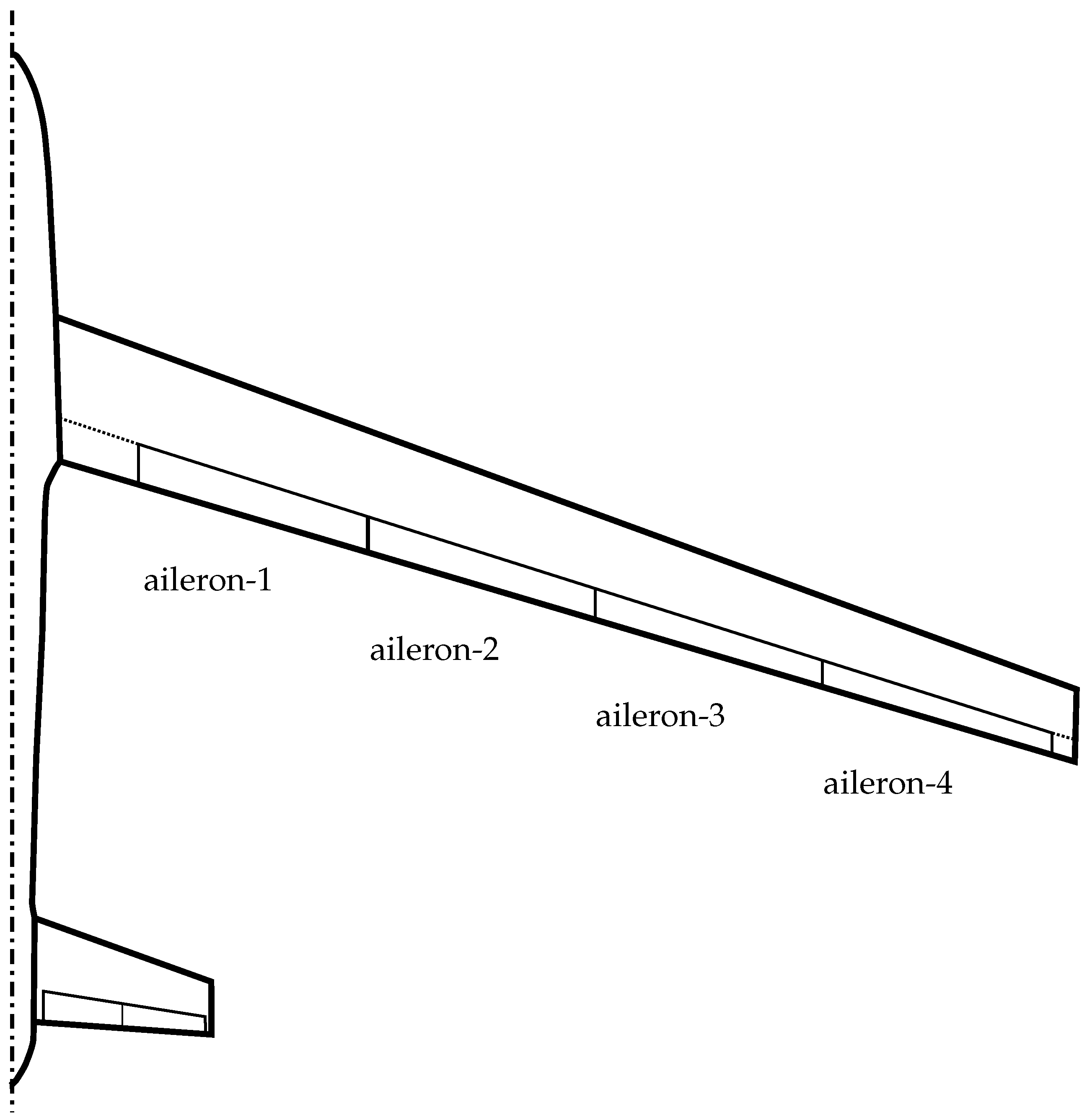
Figure 2 depicts the aileron layout. The wing is equipped with four ailerons located between and of the semi-span. The spanwise length of each control surface is of the semi-span and the hinge line is situated at of the local chord.
The active flutter suppression is performed by means of a rotary actuator situated at approximately of the semi-span on each wing. The final position of the actuators is a result of a sensitivity study performed by Wuestenhagen et al. [20]. The inertia of the actuators has been used as an additional degree of freedom to affect the aeroelastic behaviour of the UAV. The position has been chosen in such a way that the symmetric and antisymmetric flutter mechanisms are well separated in terms of flutter frequency and speed. This measure is aimed at simplifying the controller design for flutter suppression.
For effective flutter suppression, the drive must meet strict requirements regarding the actuation frequency and the phase lag leading to a relatively large component design. As a result, the actuator cannot be installed inside the wingbox and must be mounted below the wing. The computer aided design (CAD) rendering of a part of the wing with the attached actuator is shown in Figure 3. The actuator (black) drives the outermost control surface of the wing via a rod (blue). The assembly is housed in a fairing to reduce aerodynamic drag. A rectangular tube is mounted on the side of the fairing. It is aligned in flow direction and contains a weight (red). The aeroelastic characteristics of the UAV equipped with the flutter wing can be adjusted by shifting the weight along the tube.
A simplified actuator geometry is derived to take the aerodynamic influence of the actuator into account. Figure 4 compares the original CAD model with the simplified surface geometry used for the CFD simulations. Furthermore, the rectangular tube is omitted within the CFD modeling since its aerodynamic influence is expected to be negligible.
The following study analyzes two UAV configurations. While the FLEXOP baseline configuration (FBC) neglects the aerodynamic influence of the flutter suppression actuators, the FLEXOP actuator configuration (FAC) takes their influence into account.
3.2. Finite Element Model
The elasto-dynamic behaviour of the aircraft depending on the stiffness and mass distribution is modeled by means of the finite element (FE) method of MSC/NASTRAN [21]. A high-fidelity half model representation comprising beam, shell and solid elements is used. Therefore, the classical laminate theory [22] is employed to describe the anisotropic stiffness properties of the shell elements with respect to the modeling of the composite structures. To avoid stiffness deviations caused by shell offsets, each structural component is set up as a single part. In an additional assembly process, the structural parts are connected via elements representing joints such as adhesive bonds and screw connections. The advantage of this approach is a highly accurate representation of the components masses. Fuselage and empennage are modeled in a simplified manner as beam and mass elements. All aircraft components are connected via rigid elements as represented in Figure 5.
The FEM modeling of the ailerons is depicted in Figure 6. The control surfaces are designed as a sandwich and are attached to the rear spar at two points with a fixed and a floating bearing. To take the stiffness of the ailerons into account, skin and core are modelled with shell and solid elements. The rotational degree of freedom along the hinge line is present for each control surface. The aileron support is provided by the servo connection via the flap-rod and the servo lever arm. Bearings are defined between the servo lever arm, the flap-rod and the aileron mounting point so that the actuation kinematics is modelled accurately and the effects of the ailerons on the structural dynamics are taken into account.
Furthermore, the MSC/NASTRAN implementation of DLM [23] is used to generate unsteady aerodynamic loads. The applied doublet lattice representation of the FLEXOP UAV is shown in Figure 7.
An interface is implemented to exchange displacement and load information between the structural and aerodynamic models. Therefore, the half-wing is divided into 60 sections of equal span width. A FE representation of a wing section is shown in Figure 8a. Each section consists of 7 reference nodes located along the wing section camberline as shown in Figure 8b. The modal displacements are interpolated from the reference nodes (blue in Figure 8a) to the doublet lattice by thin-plate spline (TPS) interpolation [24]. To introduce the aerodynamic load into the structure, it is first mapped using TPS technique from the doublet grid to the reference nodes. Then it is transferred by rigid connections (black) to the master node in the middle of the section. Eventually, the load is introduced from the master node into the the main and rear spar via rigid interpolation elements (cyan) to avoid artificial stiffening.
The eigenmodes of the aircraft are computed by means of the MSC/NASTRAN-implementation of the Lanczos algorithm [25]. As a free-flying aircraft is investigated, only symmetry boundary conditions have to be defined. Symmetric or antisymmetric eigenmodes are enforced by clamping the relevant degrees of freedom as defined in Table 1. Translational and rotational degrees of freedom are denoted by U and respectively. The indices specify the coordinate direction of the corresponding degree of freedom.
The first six eigenmodes correspond to rigid body motions. They are generated for SD-CFD-based analysis purposes by translating and rotating the UAV geometry around the x-, y- and z-axes. The elastic eigenmodes (modes 7–16) along with their associated natural frequency are illustrated in Figure 9. For illustration purposes the modes are rescaled such that the maximum deflection amplitude is .
3.3. CFD Setup
A half model of the aircraft is used for the SD-CFD investigations. The structured grid is generated using ICEM CFD HEXA [26]. A multi-block topology approach is used. The chosen blocking strategy allows the actuator geometry to be included for aerodynamic as well as aeroelastic investigations. The antisymmetric boundary condition for SD-CFD introduced in [27] is applied at the symmetry plane to simulate antisymmetric mode deflections by means of a half-model CFD grid. The computational domain is shown in Figure 10. The symmetry plane is depicted in blue and the far-field boundary condition is shown in red.
The distance to the far-field in x-direction is set to 15 and 14 semi-spans upstream and downstream of the aircraft, respectively. The far-field in y- and z-directions is chosen to be at a distance of 15 semi-spans.
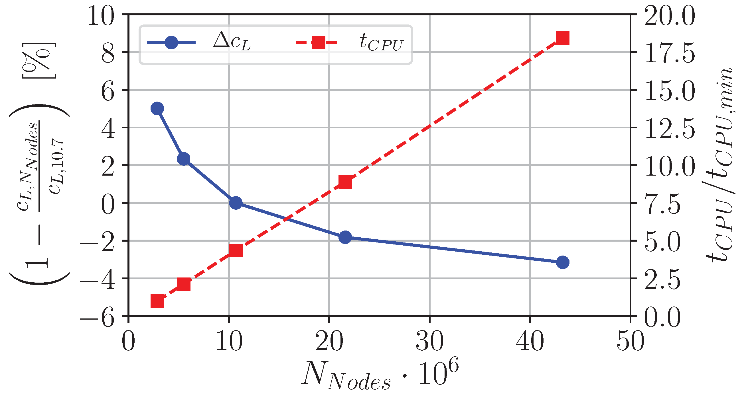
A grid sensitivity study is carried out to ensure an independence of the CFD solution from the grid resolution. Since a large number of CPU-intensive simulations has to be performed, the grid resolution should provide a sufficient solution quality with reasonable computational effort. Thus, steady-state CFD solutions based on grids with different resolutions are assessed with regard to the convergence trend over the number of cells. The Euclidean norm of the density change over an iteration normalized with the respective value after the first iteration is used as a termination criterion for all simulations. Therefore, a termination criterion of is used for the sensitivity study. Five grids with different resolutions comprising approx. , , , and million cells are compared. Figure 11 shows the lift coefficient increment for different grid resolutions with respect to the medium resolution with million cells.
A relatively big change in the lift coefficient is observed when the number of cells is increased from to million cells. A further increase of the number of cells in the domain leads only to a slight increase of the lift coefficient on the one hand and to a significant rise of the computational effort on the other hand. Furthermore, a closer look at local -distributions at different spanwise positions of the wing shows that increasing the resolution leads only to minor changes of in the front area of the wing suction side. Exemplarily, a comparison of the chordwise -distribution at , and for different grid resolutions is shown in Figure 12.
On the basis of the aforementioned considerations, the CFD grid with medium resolution and million FV-cells is chosen for further aeroelastic investigations.
The first grid-line is placed at a normal distance of mm from the wall. It is approximately . The wing geometry is discretized with 113 chordwise and 129 spanwise cells. The surface grid of FAC is shown in Figure 13.
Perturbed grids are required as an input for the computation of the -terms depicted in Equation (9). Therefore, the original surface CFD grid is deformed with respect to the shape of each structural mode. To ensure comparability with the DLM results, the same modal displacement information is used for the SD-CFD model. Thus, the modal displacements from the FE reference nodes are mapped to the CFD surface grid using TPS interpolation. Subsequently, the outer region of the computational domain is adjusted according to the surface grid deflection. This task is accomplished by means of the transfinite interpolation [28]. The amplitudes of the structural modes have to be rescaled to meet linearity requirements.
A sensitivity study is conducted to eliminate possible adverse effects of the deflection amplitude on the SD-CFD solution that may result from rounding errors or deteriorated grid quality. The perturbed grids based on different amplitude scalings of a modal shape are generated for several modes under investigation. The scalings are characterized by the maximum deflection amplitude . Subsequently, SD-CFD simulations are performed for each scaling to calculate oscillatory aerodynamic derivatives. A range of is found, where the oscillatory aerodynamic derivatives are linear over for all investigated modal shapes and reduced frequencies. Figure 14 shows exemplarily the real and imaginary parts of and across for mode 8 and as well as mode 22 and . It can be seen that oscillatory aerodynamic derivatives normalized with the maximum deflection amplitude do not vary over the range mm. This is also the case for the other modes and frequencies. Thus, for all SD simulations the mode shapes are rescaled such that the maximum deflection does not exceed 1 mm or approximately .
4. Results
This section presents the results of the conducted flutter analysis using SD-CFD-based and modal FE data. In addition, the SD-CFD-based results are compared with the results generated with MSC/NASTRAN-DLM in terms of the predicted flutter boundary and -trends. Furthermore, the aerodynamic influence of the actuator on the aeroelastic behaviour of the UAV is discussed.
4.1. Results of the Steady State CFD Simulation
The aeroelastic study is carried out for flight conditions corresponding to the envisaged flutter flight test. The load factor is . The Mach number of is chosen that approximately corresponds to the Mach number of the envisaged flight test. The density is , which corresponds to an altitude of 800 m above MSL according to the international standard atmosphere model. Trim calculations, performed by MSC/NASTRAN, yielded a trim condition at an angle of incidence of . This value is used throughout all simulations. Moreover, the predicted deformation of the wing due to static aeroelasticity at -flight is marginal. The deflection in z-direction at the wing tip does not exceed of the semi-span. Thus, the static wing deformation is neglected within this study and the jig shape is taken as the reference shape of the aircraft to reduce the modelling complexity.
The result of the steady-state AER-Eu-simulation at the previously described freestream conditions is used as a reference state for the SD simulations. Steady aerodynamic loads are visualized by means of the pressure coefficient contour plot in Figure 15. The pressure coefficient distribution is characteristic for a low-mach-number aircraft with a high-aspect-ratio wing. Suction regions can be observed at the upper side of the wing.
4.2. Aeroelastic Behavior of the Baseline Configuration
The aeroelastic analysis is performed in terms of modal coordinates. A set of the first 16 eigenmodes is used for all investigations. Unsteady aerodynamics is evaluated by means of SD- as well as DLM-model at the reduced frequencies of . In the case of the SD-based approach, the generalized aerodynamic forces are computed according to Equation (10). Subsequently, the flutter equation is solved by means of the well-established p-k method [29] for the speed range from to . For all results presented below the structural damping is set to zero.
The flutter analysis yields two aeroelastic modes which become unstable in the speed range of interest. The corresponding root locus plot is shown in Figure 16. In addition, V-f and V-g trends are presented in Figure 17.
The symmetric mode 9 and the antisymmetric mode 8 become undamped at and , respectively. The frequency at the stability boundary is for mode 9 and for mode 8. An overview of the quantities characterizing the flutter boundaries is provided in Table 2.
A flutter mode can be considered as a linear combination of structural eigenmodes with complex amplitude ratios. Absolute values of the amplitude ratios describe the participation of structural eigenmodes in a flutter mechanism. The velocity trends of these quantities are shown in Figure 18. Velocity trends of modal amplitude ratios representing participation of strucural eigenmodes in both flutter mechanisms are shown in Figure 18. At low velocities, the aeroelastic degree of freedom 9 can be mostly attributed to the first symmetric wing torsion (see Figure 9c). As the air speed increases, the ratio of the first symmetric wing bending raises significantly. When approaching the flutter speed, the amount of the second symmetric wing bending becomes also considerable. Hence, the symmetric flutter mechanism is mostly dominated by the coupling of the first and second symmetric wing bending with the first symmetric wing torsion. The aeroelastic degree of freedom 8 almost coincides with the first antisymmetric wing bending (see Figure 9b) under wind-off conditions. With increasing air speed, the first antisymmetric wing torsion (see Figure 9d) gains influence. Furthermore, this also applies to a lesser extent to the rigid body mode associated with the rolling motion. Thus, the antisymmetric flutter mechanism is prevailed by the interaction of the first antisymmetric wing bending, first antisymmetric wing torsion and the roll motion.
If solely elastic modes are considered by the p-k-method, only the symmetric flutter mechanism occurs. Thus, taking the rolling motion into account is crucial for the aeroelastic mode 8 to become unstable in the velocity range of the flight tests.
The magnitudes of the complex-valued aeroelastic modes 9 and 8 are illustrated in Figure 19. They are rescaled to of the magnitudes obtained by the p-k-method for illustration purposes.
4.3. Sensitivity of the Flutter Limits Concerning the Size of the GAF Dataset
The sensitivity of the flutter limits to the number of considered structural eigenmodes as well as the number of reduced frequencies is investigated. Figure 20 shows the variation of the relative difference of flutter speeds and flutter frequencies to the reference values over . The reference values for flutter speeds and flutter frequencies have been calculated based on the full set of 30 eigenmodes and 10 reduced frequencies. On the basis of 16 structural eigenmodes, it is possible to calculate the flutter limit with a deviation of less than with regard to the flutter speed and with regard to the flutter frequency for both flutter modes. Based on this study, a set containing the first 16 structural eigenmodes is sufficient to accurately capture the flutter behavior of the aircraft. The sensitivity of flutter limits to the number of considered reduced frequencies is shown in Figure 21 for the SD-CFD-based aeroelastic investigation. The reference values are again based on calculations considering the full set of 30 eigenmodes and 10 reduced frequencies. The subset of data at the lowest and highest reduced frequencies is used as a starting point. Flutter speeds are recomputed by adding data evaluated at the next higher reduced frequency to the data-subset. The flutter speeds as well as frequencies are converged for both flutter modes by taking into account five reduced frequencies . Therefore, the employed dataset can be regarded as sufficiently resolved across the range to ensure an accurate flutter analysis for this low-speed aircraft configuration.
To reduce the number of required simulations for the FAC, the matrix evaluated for the first 16 eigenmodes at 6 reduced frequencies is used as the input for all flutter investigations employing the p-k-method.
4.4. Comparison of SD-CFD-Based and DLM-Based Results
The results of the flutter analysis based on the SD-CFD-model are juxtaposed against the results based on a linear-potential-theory-method. For this purpose, the data are computed by means of MSC/NASTRAN-DLM. The comparison of the most relevant elements for both flutter mechanisms is presented in Figure 22. Here, the aerodynamic interactions of symmetric or antisymmetric first wing bending (structural modes 7 or 8) and wing torsion (structural modes 9 or 10) are represented in the complex plane. A good agreement of characteristic shapes is observed across all elements. However, for low there is an offset in the real-part between the SD-CFD-based and the DLM-based results. Moreover, the difference in imaginary and real parts increases with increasing .
Subsequently, the equation of aeroelasticity is solved once again by means of the p-k-method using DLM-based data. The results are consistent to the SD-CFD-based investigation yielding unstable behaviour of aeroelastic degrees of freedom 9 and 8. Nevertheless, deviations in lead to slightly different frequency and damping ratio trends of the flutter modes (see Figure 23). In general, while the agreement of the frequency and damping for mode 9 is very good, the deviation for mode 8 is higher. At lower speeds, damping values are well matched for both degrees of freedom. However, the analysis based on the DLM model results in higher damping for mode 9 and 8 starting at and , respectively, compared to the SD-CFD-based approach. As a consequence, the flutter boundaries are shifted towards higher velocities for the DLM modeling in comparison to the SD-CFD modeling. Hence, SD-CFD-based results yield lower flutter speeds in contrast to the DLM-based results.
Moreover, deviations with regard to the frequency trend of mode 8 are observed comparing the two methods for aerodynamic modeling. For DLM-based aerodynamics, the eigenfrequency of the aeroelastic degree of freedom 8 is almost constant up to . With higher speed the frequency decreases. In contrast, the frequency trend obtained by the SD-CFD approach increases at lower velocities and decreases at higher velocities showing a maximum at approximately . Therefore, mainly the aforementioned difference leads to a frequency deviation at the flutter limit for mode 8.
The frequency trend of the aeroelastic degree of freedom 9 obtained by DLM matches with that obtained by SD-CFD up to . Hence, the deviation in the flutter frequency of mode 9 is solely due to the difference in the damping behaviour and, thus, also in the flutter velocity predicted by DLM and SD-CFD aerodynamics. Table 3 gives an overview of the computed stability limits when using both models for the unsteady aerodynamics. The deviations of the flutter limits are expressed as a percentage of the SD-CFD-based results.
It is expected that the results of SD-CFD provide higher accuracy compared with DLM since SD-CFD as a high-fidelity-method takes the effects of thickness and aerodynamic interferences into account.
4.5. Aeroelastic Influence of the Actuator
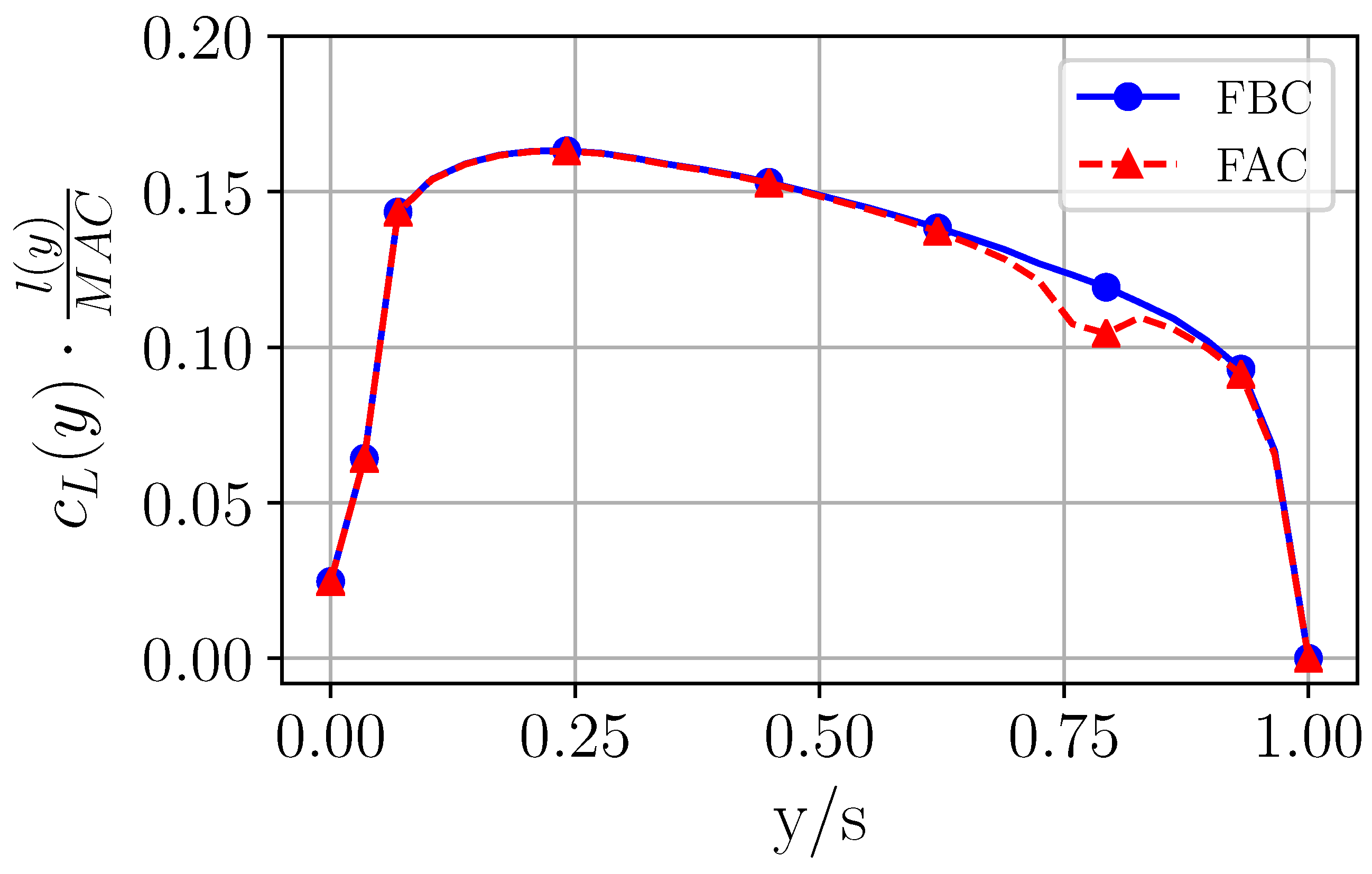
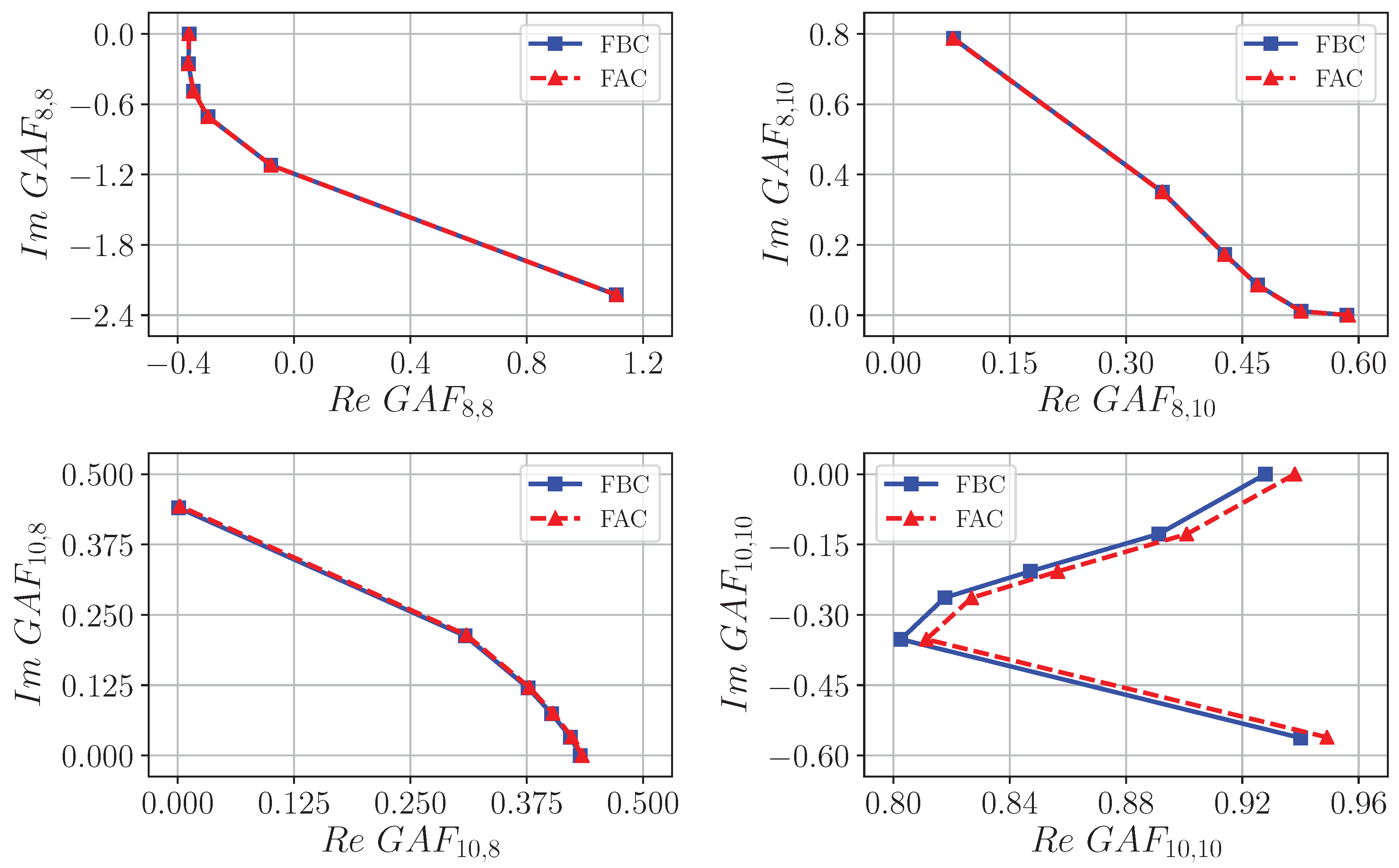
To complement the sensitivity study in [20] as well as to exclude negative effects on flutter controllability, also the influence of the actuators on unsteady aerodynamics is investigated. Here, the advantage of SD-CFD methods to capture complex flow phenomena and thickness effects is exploited to address the problem. A steady-state simulation of FAC is carried out for the same flow conditions as for the FBC. The difference of the spanwise lift distribution due to the presence of the actuator is shown in Figure 24. A distinct breakdown of the aerodynamic load can be observed at the location of the actuator for the FAC compared to the FBC.
Unsteady simulations are conducted for the range of reduced frequencies as justified by the aforementioned sensitivity study. As the first step, the derivative of with respect to the y-direction is considered (see Figure 25). This quantity can be interpreted as the local wing section contribution to . Exemplarily, structural modes 7 and 9 are taken into account that are most relevant for the symmetric flutter mechanism. The unsteady aerodynamics is evaluated for , which is close to the flutter frequency.
It is interesting to notice that the wing section contribution to all considered modal generalizations is almost zero up to approx. of the semi-span. The absolute value of the contribution increases to the outboard of the wing. As expected, deviations in the real as well as imaginary part of the derivative can be observed at the actuator position when comparing the FAC and the FBC. Furthermore, the generalization involving unsteady loads due to the harmonic motion of mode 7 (elements with ) leads to large differences in the real part compared to other mode generalizations. However, the largest encountered deviations can be regarded as minor in the context of aeroelastic investigations.
Subsequently, also elements representing the interaction of symmetric and antisymmetric modes of wing bending and torsion that determine both flutter mechanisms are considered. The complex plane representation of relevant elements is shown in Figure 26. As expected, the aforementioned differences between the FAC and the FBC in terms of the spanwise wing section contribution to generalized aerodynamic forces lead to deviations in elements. Although the modification of the generalized aerodynamic forces by the actuator over the considered range of the reduced frequencies is discernible, it can be regarded as marginal.
Finally, the aerodynamic influence of the actuator is evaluated using conventional linear flutter analysis. The analysis is conducted employing the p-k-method. The same dimensionality of the dataset regarding the number of reduced frequencies and structural modes is used as the input for the analysis of the FAC and the FBC. The resulting velocity trends of the damping ratio and frequency for both flutter modes are depicted in Figure 27.
The overview of resulting stability limits is presented in Table 4. The deviation is well below one percent for both the flutter frequency and the speed when comparing the FAC with the FBC. It can, therefore, be concluded that the aerodynamic influence of the actuator on the flutter behaviour of the aircraft is negligible.
5. Conclusions
The scope of this work is the comprehensive aeroelastic analysis of the FLEXOP demonstrator UAV using the small disturbance CFD (SD-CFD) approach for unsteady aerodynamic modeling. The general SD-based methodology for flutter prediction is outlined and the modelling of the UAV using FE and CFD is presented. Sensitivity studies are carried out, which are used to identify suitable parameters for SD-CFD calculations and the required database size for flutter analysis. The SD-CFD-based flutter analysis is performed yielding two aeroelastic modes that become unstable in the speed range of interest.
The focus of this work is on the application of SD-CFD for the modelling of unsteady aerodynamic loads. Nevertheless, a comparison is drawn between SD-CFD-based aerodynamic and linear-potential-theory-based DLM modelling to gain confidence in the flutter behaviour of the aircraft. The comparative analysis is made on the basis of relevant generalized aerodynamic forces and the results of the subsequent flutter analysis. The employed p-k method yields consistent results regarding the flutter mechanisms across both models for unsteady aerodynamics. Nevertheless, the SD-based flutter results are more conservative with regard to the predicted stability limits. SD-CFD results are expected to provide higher accuracy due to the full aerodynamic shape representation, thus including all interference effects. Furthermore, the use of SD-CFD facilitates the assessment of the influence of the actuator fairing on the unsteady aerodynamics and thus on the flutter behaviour of the UAV. The investigation shows that the unsteady aerodynamic effects due to the presence of the actuator fairing are negligible.
The future work will include further aeroelastic investigations of the flutter demonstrator using the calibrated structural model after the ground vibration test. In addition, aeroelastic effects due to the wing flexibility will be a matter of forthcoming study.
Author Contributions
Conceptualization, V.R.; methodology, V.R., A.V. and A.H.; software, V.R. and A.V.; validation, V.R.; formal analysis, V.R. and A.V.; investigation, V.R., A.V. and A.H.; data curation, V.R.; writing—original draft preparation, V.R.; writing—review and editing, V.R.; visualization, V.R., A.V. and A.H.; supervision, C.B. and M.H.; project administration, C.B. and M.H.; funding acquisition, C.B. and M.H.
Funding
The research leading to these results is part of the FLEXOP project. This project has received funding from the European Union’s Horizon 2020 research and innovation programme under grant agreement No 636307.
Acknowledgments
The authors gratefully acknowledge the Gauss Centre for Supercomputing e.V. (www.gauss-centre.eu) for funding this project by providing computing time on the Linux-Cluster at Leibniz Supercomputing Centre (www.lrz.de).
Conflicts of Interest
The authors declare no conflict of interest.
References
- Scheelhaase, J.; Grimme, W.; O’Sullivan, M.; Naegler, T.; Klötzke, M.; Kugler, U.; Scheier, B.; Standfuß, T. Klimaschutz im Verkehrssektor—Aktuelle Beispiele aus der Verkehrsforschung. Wirtschaftsdienst 2018, 98, 655–663. [Google Scholar] [CrossRef]
- Price, M.; Raghunathan, S.; Curran, R. An Integrated Systems Engineering Approach to Aircraft Design. Prog. Aerosp. Sci. 2006, 42, 331–376. [Google Scholar] [CrossRef]
- Hall, K.C.; Crawley, E.F. Calculation of Unsteady Flows in Turbomachinery Using the Linearized Euler Equations. AIAA J. 1989, 27, 777–787. [Google Scholar] [CrossRef]
- Hall, K.C.; Clark, W.S. Linearized Euler Predictions of Unsteady Aerodynamic Loads in Cascades. AIAA J. 1993, 31, 540–550. [Google Scholar] [CrossRef]
- Kreiselmaier, E.; Laschka, B. Small Disturbance Euler Equations: Efficient and Accurate Tool for Unsteady Load Prediction. J. Aircr. 2000, 37, 770–778. [Google Scholar] [CrossRef]
- Pechloff, A.; Laschka, B. Small Disturbance Navier-Stokes Method: Efficient Tool for Predicting Unsteady Air Loads. J. Aircr. 2006, 43, 17–29. [Google Scholar] [CrossRef]
- Iatrou, M. Ein Navier-Stokes-Verfahren Kleiner Störungen Für Instationäre Vorgänge—Anwendung auf Transportflugzeuge. Ph.D. Thesis, Technische Universität München, München, Germany, 2010. [Google Scholar]
- Dufour, G.; Sicot, F.; Puigt, G.; Liauzun, C.; Dugeai, A. Contrasting the Harmonic Balance and Linearized Methods for Oscillating-Flap Simulations. AIAA J. 2010, 48, 788–797. [Google Scholar] [CrossRef] [Green Version]
- Thormann, R.; Widhalm, M. Linear-Frequency-Domain Predictions of Dynamic-Response Data for Viscous Transonic Flows. AIAA J. 2013, 51, 2540–2557. [Google Scholar] [CrossRef]
- Weishäupl, C.; Laschka, B. Small Disturbance Euler Simulations for Delta Wing Unsteady Flows due to Harmonic Oscillations. J. Aircr. 2004, 41, 782–789. [Google Scholar] [CrossRef]
- Da Ronch, A.; McCracken, A.; Badcock, K.J.; Widhalm, M.; Campobasso, M.S. Linear Frequency Domain and Harmonic Balance Predictions of Dynamic Derivatives. J. Aircr. 2013, 50, 694–707. [Google Scholar] [CrossRef] [Green Version]
- Revalor, Y.; Daumas, L.; Forestier, N. Industrial Use of CFD for Loads and Aero-Servo-Elastic Stability Computations at Dassault Aviation. In Proceedings of the 14th International Forum on Aeroelasticity and Structural Dynamics, Paris, France, 26–30 June 2011. [Google Scholar]
- Winter, M.; Heckmeier, F.M.; Breitsamter, C. CFD-based Aeroelastic Reduced-Order Modeling Robust to Structural Parameter Variations. Aerosp. Sci. Technol. 2017, 67, 13–30. [Google Scholar] [CrossRef]
- Albano, E.; Rodden, W.P. A Doublet-Lattice Method for Calculating Lift Distributions on Oscillating Surfaces in Subsonic Flows. AIAA J. 1969, 7, 279–285. [Google Scholar] [CrossRef]
- Giesing, J.P.; Kalman, T.P.; Rodden, W.P. Subsonic Unsteady Aerodynamics for General Configurations. In Proceedings of the 10th Aerospace Sciences Meeting, San Diego, CA, USA, 17–19 January 1972. [Google Scholar]
- Rodden, W.P.; Giesing, J.P.; Kalman, T.P. Refinement of the Nonplanar Aspects of the Subsonic Doublet-Lattice Lifting Surface Method. J. Aircr. 1972, 9, 69–73. [Google Scholar] [CrossRef]
- Wright, J.R.; Cooper, J.E. Introduction to Aircraft Aeroelasticity and Loads; Aerospace series; Wiley: Chichester, UK, 2008. [Google Scholar]
- Fleischer, D. Verfahren Reduzierter Ordnung zur Ermittlung Instationärer Luftkräfte. Ph.D. Thesis, Technische Universität München, München, Germany, 2014. [Google Scholar]
- Rozov, V.; Hermanutz, A.; Breitsamter, C.; Hornung, M. Aeroelastic Analysis of a Flutter Demonstrator with a Very Flexible High-Aspect-Ratio Swept Wing. In Proceedings of the 17th International Forum on Aeroelasticity and Structural Dynamics, Como, Italy, 25–28 June 2017. [Google Scholar]
- Wuestenhagen, M.; Kier, T.; Meddaikar, Y.M.; Pusch, M.; Ossmann, D.; Hermanutz, A. Aeroservoelastic Modeling and Analysis of a Highly Flexible Flutter Demonstrator. In 2018 Atmospheric Flight Mechanics Conference; American Institute of Aeronautics and Astronautics: Reston, VA, USA, 2018. [Google Scholar] [CrossRef]
- MSC. Software. Release Guide; MSC.Software Corporation: Newport Beach, CA, USA, 2018. [Google Scholar]
- Gürdal, Z.; Haftka, R.T.; Hajela, P. Design and optimization of laminated composite materials; A Wiley-Interscience Publication, Wiley: New York, NY, USA, 1999. [Google Scholar]
- MSC. Software. Aeroelastic Analysis User’s Guide; MSC.Software Corporation: Newport Beach, CA, USA, 2018. [Google Scholar]
- Duchon, J. Splines Minimizing Rotation-Invariant Semi-Norms in Sobolev Spaces. Construct. Theory Funct. Sev. Var 1977, 85–100. [Google Scholar]
- Lanczos, C. An Iteration Method for the Solution of the Eigenvalue Problem of Linear Differential and Integral Operators. J. Res. Natl. Bur. Stand. 1950, 45, 255–282. [Google Scholar] [CrossRef]
- ANSYS. ANSYS ICEM CFD User Manual; ANSYS, Inc.: Canonsburg, PA, USA, 2012. [Google Scholar]
- Rozov, V.; Winter, M.; Breitsamter, C. Antisymmetric Boundary Condition for Small Disturbance CFD. J. Fluids Struct. 2019, 85, 229–248. [Google Scholar] [CrossRef]
- Gordon, W.J.; Hall, C.A. Construction of Curvilinear Co-Ordinate Systems and Applications to Mesh Generation. Int. J. Nume. Methods Eng. 1973, 7, 461–477. [Google Scholar] [CrossRef]
- Hassig, H.J. An Approximate True Damping Solution of the Flutter Equation by Determinant Iteration. J. Aircr. 1971, 8, 885–889. [Google Scholar] [CrossRef]
Figure 1.
Planform of the FLEXOP UAV based on [19].
Figure 1.
Planform of the FLEXOP UAV based on [19].

Figure 2.
Aileron layout of the FLEXOP configuration.

Figure 3.
CAD rendering of the flutter suppression actuator.

Figure 4.
CAD model (left) and the CFD model (right) of the actuator.

Figure 5.
FE model of the FLEXOP UAV.

Figure 6.
FEM modeling of the ailerons.

Figure 7.
Doublet lattice representing FLEXOP UAV.

Figure 8.
Aero-structural load interface.

Figure 9.
First ten structural elastic eigenmodes. Displacement and contours are given as . Labels “sym” and “asym” denote symmetric and antisymmetric modes, respectively.
Figure 9.
First ten structural elastic eigenmodes. Displacement and contours are given as . Labels “sym” and “asym” denote symmetric and antisymmetric modes, respectively.

Figure 10.
Discretized computational domain of the FLEXOP half model with the medium resolution.

Figure 11.
Variation of the lift coefficient and normalized CPU time for different grid resolutions specified by the number of cells . The medium resolution is taken as the reference.
Figure 11.
Variation of the lift coefficient and normalized CPU time for different grid resolutions specified by the number of cells . The medium resolution is taken as the reference.

Figure 12.
Comparison of chordwise -distributions for different grid resolutions of the FBC.

Figure 13.
Surface grid of FAC.

Figure 14.
Comparison of and across for mode 8 and as well as mode 22 and .

Figure 15.
Contour plot of the steady-state distribution at and (AER-Eu).

Figure 16.
Root locus of the FBC for the first 16 eigenmodes and a speed range from to .

Figure 17.
Frequency and damping trends of the FBC for the first 16 eigenmodes and a speed range from to .
Figure 17.
Frequency and damping trends of the FBC for the first 16 eigenmodes and a speed range from to .

Figure 18.
Velocity trends of the absolute values of the modal amplitude ratios representing the participation of the strucural eigenmodes.
Figure 18.
Velocity trends of the absolute values of the modal amplitude ratios representing the participation of the strucural eigenmodes.

Figure 19.
Displacement of the flutter modes. Displacement and contours are given as . Grey: non-deformed aircraft.
Figure 19.
Displacement of the flutter modes. Displacement and contours are given as . Grey: non-deformed aircraft.

Figure 20.
Sensitivity of the flutter limits with regard to the number of considered modes.

Figure 21.
Sensitivity of the flutter limits with regard to the number of considered reduced frequencies.
Figure 21.
Sensitivity of the flutter limits with regard to the number of considered reduced frequencies.

Figure 22.
Comparison of SD-CFD and DLM with regard to resulting GAF entries of the dominant flutter modes at .
Figure 22.
Comparison of SD-CFD and DLM with regard to resulting GAF entries of the dominant flutter modes at .


Figure 23.
Comparison of SD-CFD and DLM modeling with regard to the resulting behaviour of the flutter modes.
Figure 23.
Comparison of SD-CFD and DLM modeling with regard to the resulting behaviour of the flutter modes.

Figure 24.
Comparison of steady-state wing loads for the FBC and the FAC.

Figure 25.
Comparison of the FBC and the FAC with regard to the resulting wing section contribution to at .
Figure 25.
Comparison of the FBC and the FAC with regard to the resulting wing section contribution to at .


Figure 26.
Comparison of the FBC and the FAC with regard to resulting GAF entries of the dominant flutter modes at .
Figure 26.
Comparison of the FBC and the FAC with regard to resulting GAF entries of the dominant flutter modes at .


Figure 27.
Comparison of SD-CFD and DLM modeling with regard to the resulting behaviour of the flutter modes.
Figure 27.
Comparison of SD-CFD and DLM modeling with regard to the resulting behaviour of the flutter modes.


Table 1.
Boundary conditions at the plane of symmetry of the aircraft.
| Symmetric Boundary Condition | Antisymmetric Boundary Condition |
|---|---|
Table 2.
Flutter boundaries of FBC.
| Mode 9 | Mode 8 | |
|---|---|---|
Table 3.
Overview of the predicted flutter limits based on SD-CFD and DLM modeling.
| Mode 9 | Mode 8 | ||||
|---|---|---|---|---|---|
| SD-CFD | DLM | SD-CFD | DLM | ||
| − | − | ||||
| − | − | ||||
| − | − | ||||
Table 4.
Overview of the predicted flutter limits of the FBC and the FAC based on SD-CFD.
| Mode 9 | Mode 8 | ||||
|---|---|---|---|---|---|
| FBC | FAC | FBC | FAC | ||
| − | − | ||||
| − | − | ||||
| − | − | ||||
© 2019 by the authors. Licensee MDPI, Basel, Switzerland. This article is an open access article distributed under the terms and conditions of the Creative Commons Attribution (CC BY) license (http://creativecommons.org/licenses/by/4.0/).
Share and Cite
MDPI and ACS Style
Rozov, V.; Volmering, A.; Hermanutz, A.; Hornung, M.; Breitsamter, C. CFD-Based Aeroelastic Sensitivity Study of a Low-Speed Flutter Demonstrator. Aerospace 2019, 6, 30. https://doi.org/10.3390/aerospace6030030
AMA Style
Rozov V, Volmering A, Hermanutz A, Hornung M, Breitsamter C. CFD-Based Aeroelastic Sensitivity Study of a Low-Speed Flutter Demonstrator. Aerospace. 2019; 6(3):30. https://doi.org/10.3390/aerospace6030030
Chicago/Turabian StyleRozov, Vladyslav, Andreas Volmering, Andreas Hermanutz, Mirko Hornung, and Christian Breitsamter. 2019. "CFD-Based Aeroelastic Sensitivity Study of a Low-Speed Flutter Demonstrator" Aerospace 6, no. 3: 30. https://doi.org/10.3390/aerospace6030030
Note that from the first issue of 2016, this journal uses article numbers instead of page numbers. See further details here.