Verification of Boundary Conditions Applied to Active Flow Circulation Control


VZLU—Czech Aerospace Research Centre, 199 05 Prague, Czech Republic
*
Author to whom correspondence should be addressed.
Aerospace 2019, 6(3), 34; https://doi.org/10.3390/aerospace6030034
Submission received: 30 November 2018
/
Revised: 2 March 2019
/
Accepted: 4 March 2019
/
Published: 8 March 2019
(This article belongs to the Special Issue 8th EASN-CEAS Workshop on Manufacturing for Growth and Innovation)
Abstract
:Inclusion of Active Flow Control (AFC) into Computational Fluid Dynamics (CFD) simulations is usually highly time-consuming and requires extensive computational resources and effort. In principle, the flow inside of the fluidic AFC actuators should be incorporated into the problem under consideration. However, for many applications, the internal actuator flow is not crucial, and only its effect on the outer flow needs to be resolved. In this study, the unsteady periodic flow inside the Suction and Oscillatory Blowing (SaOB) actuator is analyzed, using two CFD methods of ranging complexity (URANS and hybrid RANS-LES). The results are used for the definition and development of the simplified surface boundary condition for simulating the SaOB flow at the actuator’s exit. The developed boundary condition is verified and validated, in the case of a low-speed airfoil with suction applied on the upper (suction) side of the airfoil and oscillatory blowing applied on the lower (pressure) side, close to the trailing edge—a fluidic Gurney flap. Its effect on the circulation is analyzed and compared to the experimental data.
1. Introduction
Active Flow Control (AFC) is considered to be a useful technique in enhancing the performance of existing designs. However, it is challenging to include AFC when already in the design phase. The reason for this is the high geometric complexity of the AFC flow actuators (jets, suction holes, internal structure, and tubing) which should be incorporated, in the case of full resolution. Consequently, the required resources increase due to various reasons. First, it adds complexity to the computational grids, which, in the case of full resolution, need to include the internal shape of the actuators themselves. Furthermore, a heavy workload is needed during the grid generation process, which is far from being automatic. A second, and in some sense complementary, issue is the growth of the problem size in terms of the number of grid points, which leads to increased wall-time and Central Processing Unit (CPU) resources needed to solve the problem. This is even more significant in the case of actuator arrays, where even the effort to simulate the AFC internal flows easily exceeds the typical size of the corresponding problem without AFC. Moreover, the flow is usually inherently unsteady by nature, especially in the case of pulsed or oscillatory blowing, which requires time-consuming and unsteady calculations, as well as a statistical evaluation of the results. Moreover, there might be a large time-scale separation between mean flow phenomena and the AFC actuator internal flow frequencies. While it is desirable to simplify AFC in the Computational Fluid Dynamics (CFD) simulation (i.e., to simulate the effect of AFC, rather than to spend resources on the physical modeling of the AFC system), this cannot be done without sufficient knowledge about the internal flow of the actuator or the character of the actuator exit flow [1,2].
It has become quite popular to control flows in many aeronautical, transport, and industrial applications [3,4,5]. A number of computational studies rely on a uniform flow field at the AFC device exit [6,7,8,9,10]. It is evident that a realistic jet exit flow field is needed, in order to define appropriate boundary conditions [2,11,12] and to obtain physically consistent interactions between the actuator and the outer flow. This can be done by modeling the actuator geometry, or at least a significant part like the actuator exit nozzle, to enable development of the velocity profile and to obtain a more realistic flow field at the exit from the actuators [13,14,15,16]. The functional representation for the nozzle oscillatory velocity profiles of the SaOB (Suction and Oscillatory Blowing) actuator was developed in [12], which can be used as surface boundary conditions for complex AFC simulations. Although this representation was only 2D, it matched the measured velocity profile at the nozzle’s exit quite well. Moreover, a proper orthogonal decomposition, to create a reduced-order model of the actuator’s effect on the flow-field, was also studied [17] with the aid of Particle Image Velocimetry (PIV) experimental data.
Our goal is divided into several consecutive steps. First, we study the unsteady internal flow in a single SaOB actuator [18]. This is done by the CFD simulation using an Unsteady Reynolds Average Navier–Stokes (URANS) solver with a k– type turbulence model [19], and using hybrid Reynolds Average Navier–Stokes (RANS)-Large Eddy Simulation (LES) turbulence modeling [20]. The use of two approaches with different levels of complexity, validated using the experimental data [21], allows better insight and confidence in the computational methods. This approach, although still quite heavy on resources, is an alternative to the even more demanding LES simulations [22], which require a computational force that is out of reach, in most cases.
Based on the data from these CFD simulations, the unsteady inflow boundary condition for the simulation of the SaOB actuator has been defined, as briefly described previously in [23]. It is based on the use of Gaussian functions to obtain a spatial representation of the velocity field, combined with a harmonic function to represent the time evolution. The boundary condition, instead of the complex internal structure of the actuators, further enables conservation of the complexity of the problem under consideration, in a reasonable range. It is possible to save the load of millions of grid points by substitution of the internal structure of the actuator by the boundary condition at the actuator’s exit. It is also possible to consider actuator arrays and the incorporation of AFC during the design process, by this approach.
The second level of validation is presented by considering a subsonic flow around a quasi-2D airfoil with an integrated SaOB actuator. The increase of the lift was observed with the AFC active. The comparison of our CFD results with the experimental data [21] shows that the effect of the SaOB actuator was replicated in the simulation.
The structure of the paper is as follows. In Section 2, the principle of the SaOB actuator is briefly described, the computational problem is defined, and the CFD methods are presented. The data extracted from the CFD simulations are used, in Section 3, for the definition of the surface boundary condition. The mathematical background is briefly explained and the level of agreement between the data and the analytical description is presented. Section 4 covers the application of the simplified boundary condition to the case of a quasi-2D airfoil to enhance its circulation. The calculated values are compared to the experimental data. The conclusion briefly sums up the achieved results, and outlines other possible applications.
2. Characterization of the SaOB Actuator
Oscillatory blowing is an effective tool for increasing the momentum of the flow inside the boundary layer—which can be used, for example, for flow separation control. Periodic blowing through a series of narrow slots enhances the shear-layer mixing and transfer of high-momentum fluid from the outside of the shear layer to the near wall region, which delays the boundary-layer separation. In the present paper, the actuator is used as a fluidic Gurney flap to enhance airfoil circulation.
The actuator is a combination of an ejector and a bi-stable fluidic amplifier. When a jet stream from the pressure supply is ejected into a bigger conduit, a low-pressure region is created, due to entrainment (Figure 1a). The cavity behind the jet is open to the outer environment, through the suction ports. As a result, the pressure gradient between the internal jet area and the external environment causes air to be sucked into the cavity. This additional mass flow depends on the actual pressure gradient. This, on one hand, increases the total mass flow through the actuator and, on the other hand, it naturally causes suction—which can be further exploited by positioning the suction holes in a desirable area. Moreover, only the pressure source is needed. The oscillations of the flow between the right and left output slots (Figure 1b) is caused by the natural flow switching, controlled by the flow through the feedback tube connecting the control ports (control left and control right, see Figure 1b). No moving parts are needed to obtain oscillation.
The SaOB actuator is very effective, especially in the low range of the blowing momentum coefficient, (see Equation (3)), in comparison with other types of fluidic actuators (steady, pulsed blowing, sweeping jets, and so on). It can be used for many applications, from flow separation control to maneuvering [21,24].
2.1. CFD Simulation of the Isolated SaOB Actuator
The CFD simulations were focused on the internal flow-field and on the flow at the nozzle exit of the single SaOB actuator. These simulations corresponded to the bench-top test of the SaOB in the laboratory, in still-air ambient conditions [21]. The geometrical setup of the detailed actuator interior layout is shown in Figure 2.
As we can see, a realistic geometry of the SaOB actuator was utilized, and its geometrical details were fully resolved. In terms of boundary conditions, the pressure supply and suction ports were represented by the inflow boundary conditions. The total pressure, total temperature, and flow direction were prescribed at these boundaries, a boundary condition usually denoted as total states inlet or stagnation pressure condition. Flow direction was set as perpendicular to the geometry of the boundary conditions. The total pressure at the pressure supply boundary was varied, to obtain a wide range of working points for the comparison between CFD computations and the experimental data (available from [21]). The ambient atmospheric conditions were prescribed at the suction ports. The exit nozzles of the SaOB actuator were connected to the rectangular domain, which simulated the flat plate of the wind tunnel wall. To consider the effect of neighboring actuators, periodic boundary conditions were prescribed at the sides of the computational domain. The SaOB walls were represented by the adiabatic no-slip wall conditions. The outer flow freestream velocity was set to a value close to zero, to mimic the no-flow condition of the experiment, and then to 25 m/s, to study interaction with the outer flow. The boundary conditions in the CFD solver were implemented as weak boundary conditions; that is, they were imposed by the boundary flux, rather than assigned directly.
The internal grid of the SaOB actuator and of the computational domain was created in the Pointwise grid generation software. The grid was refined in the regions of interest (ejector, output nozzles, and the region in the vicinity of the actuator outputs). The hybrid grid grew from the mostly quad-dominant surface grid into the volume, to create a sufficiently fine grid representation in the boundary layer, and the unstructured tetra cells filled the rest of the volume. Due to unsteady nature of the flow and the large variation in the local velocities, it was challenging to set grid parameters a priori. Therefore, the grids were tuned according to preliminary results, to provide acceptable convergence, and , as recommended for the use of turbulence models. The computations were very expensive, in terms of computational time and resources. Therefore, a systematic grid convergence study is not presented. However, since the problem was solved in two steps (URANS and SST-DDES on a heavily-refined grid), the consistency of results is considered as a partial substitute.
The number of grid points is presented in Table 1, where the principal parts of the actuator grid are highlighted. The first cell height range was due to different settings in the centre of the SaOB central channel and in the control ports, where the velocity was much lower. The growth rate from the first cell height was set close to 1.2. While the grid had about 5.5 million grid points for the URANS campaign [25], it was uniformly refined—starting from the finer surface grid—to about 12 million, just inside the actuator, for the SST-DDES turbulence model study [26]; see Figure 3.
All simulations were carried out in a Finite Volume Navier–Stokes solver, Edge [27]. It was designed as a solver for the Navier–Stokes equations on unstructured meshes. The data structure inside the solver is edge-based, and the code was constructed as cell-vertex. It employs multi-grid and residual smoothing acceleration for steady-state problems. Moreover, the time accurate (unsteady) simulations use an implicit dual-time stepping approach, where, in each time step, a steady-like problem is converged to with a sequence of inner iterations. The maximum number of inner iterations was determined by the drop in the density residual (2 orders of magnitude), or by the maximum number of inner iterations reached (100–300, depending on the case). The spatial discretization of the convective terms relied on the Jameson-Schmidt-Turkel (JST) scalar scheme [28], which is of the second order of accuracy.
All simulations were run as a fully turbulent (i.e., no laminar region or laminar-to-turbulent transition was prescribed). The turbulence model used for the URANS simulations was Wallin & Johansson’s EARSM + Hellsten k– model [19], and the SST-DDES model, as presented in [20], was employed for the hybrid RANS-LES calculations.
The physical time step was varied for particular cases, depending on the oscillation frequency, to reach an adequate number of time steps per cycle of the blowing velocity, from one actuator’s outlet the other, while switching.
This was defined by the sampling rate. The sampling rate of the oscillation frequency was kept at a similar level for all simulated cases. Its value was high enough to obtain a smooth description of the oscillating frequency. This means that the physical time step was varied from 0.00002 s, corresponding to the lowest oscillation frequency, to 0.00001 s, for the highest oscillation frequency. This gave approximately 200 time steps per oscillation period. The typical snapshot of the flow inside the actuator is presented in Figure 4.
2.2. CFD Results and Interpretation
The main aim of this study was to obtain the time-dependent flow field variables at the SaOB actuator exit nozzle for different supply pressures. These results serve as a source of data for boundary condition definition. Furthermore, comparison between URANS with the k– model and the hybrid RANS-LES, model represented by the SST-DDES simulation, brings more confidence in the computational results.
A basic comparison can be made using the experimental results (as in [21]), where the actuator exit peak velocity and oscillation frequency were evaluated; see Figure 5. The comparison of the maximum outlet nozzle velocity and the oscillation frequency, which naturally develops due to the flow inside the actuator, is presented. The frequency range of between and was obtained; which relates to the maximum actuator outlet velocities, in the range between and .
A good agreement between the experimental data and the computational results of the URANS and hybrid RANS-LES simulations was achieved. It has to be noted that there was a certain degree of non-symmetry in the results (between the left–right actuator outputs) that was observed both in the experimental data [21] (where it can be attributed to the manufacturing tolerances of the actuators) and also in the CFD results, which is probably due to a not fully-symmetric grid and the S-shaped feedback channel. The data were averaged from both output nozzles before they were presented. More details on the evaluation of the data are given in Section 3. The linear trend between the oscillation frequency and the peak velocity at the nozzle exit was preserved for all the results mentioned here.
The velocity profile at the actuator’s exit was highly non-uniform in both directions (streamwise and spanwise), see Figure 6. This was not necessarily a drawback, since it enhanced mixing inside the boundary layer. As the velocity profile was subject to a complex flow field inside the actuator, it was necessary to accurately simulate the internal flow, capture local separations, and so on. In our case, the non-uniformity of the flow could also be attributed to the shape of the exit nozzle (see Figure 4), which deflected the flow from the streamwise direction to the perpendicular normal direction. The flow was, thus, due to its momentum attached to the outer wall, along the outlet nozzle radius.
Figure 7 shows a comparison of the SaOB actuator exit nozzles at the time instant when the peak value was achieved. While the URANS results were spatially interpolated (due to probe recording done during the simulations), the hybrid RANS-LES results showed instantaneous values from the cut through the computational domain in the same spatial position. There was no significant deviation between both peak velocity profiles, although it is possible to see some differences in the velocity profile of the ‘inactive’ actuator outlet (left outlet, in the case that the right outlet is in the peak velocity phase, and vice versa). The residuals of the flow through the nominally inactive outlet nozzle contributed to the nonzero mass flux through this outlet. However, the momentum there was relatively small. Another nice property of the velocity profile is that it was fairly self-similar for different operational states of the SaOB actuator; see Section 3. This has been observed not only in [23], for the present version of the SaOB actuator, but also in [22], for a slightly different geometry.
3. Definition of the Boundary Condition
The time-dependent flow-field variables at the actuator’s exit were extracted from the CFD simulations and approximated by the surrogate model. The main character of the flow was periodic with the frequency of the flow oscillation, corresponding to different inlet pressures into the SaOB actuator.
A wide range of usage of surrogate modeling had been seen in the field of computational science in recent decades. There are many mathematical approaches that provide surrogate modeling: Kriging, Response surface method [6], artificial neural networks [29], Gaussian processes [30], and so on. In this case, an analytical function, describing the character of the flow field, was used. More specifically, the normal and spanwise components of velocity were described as a sum of the two-dimensional Gaussian functions multiplied by the sine function; the generic form is:
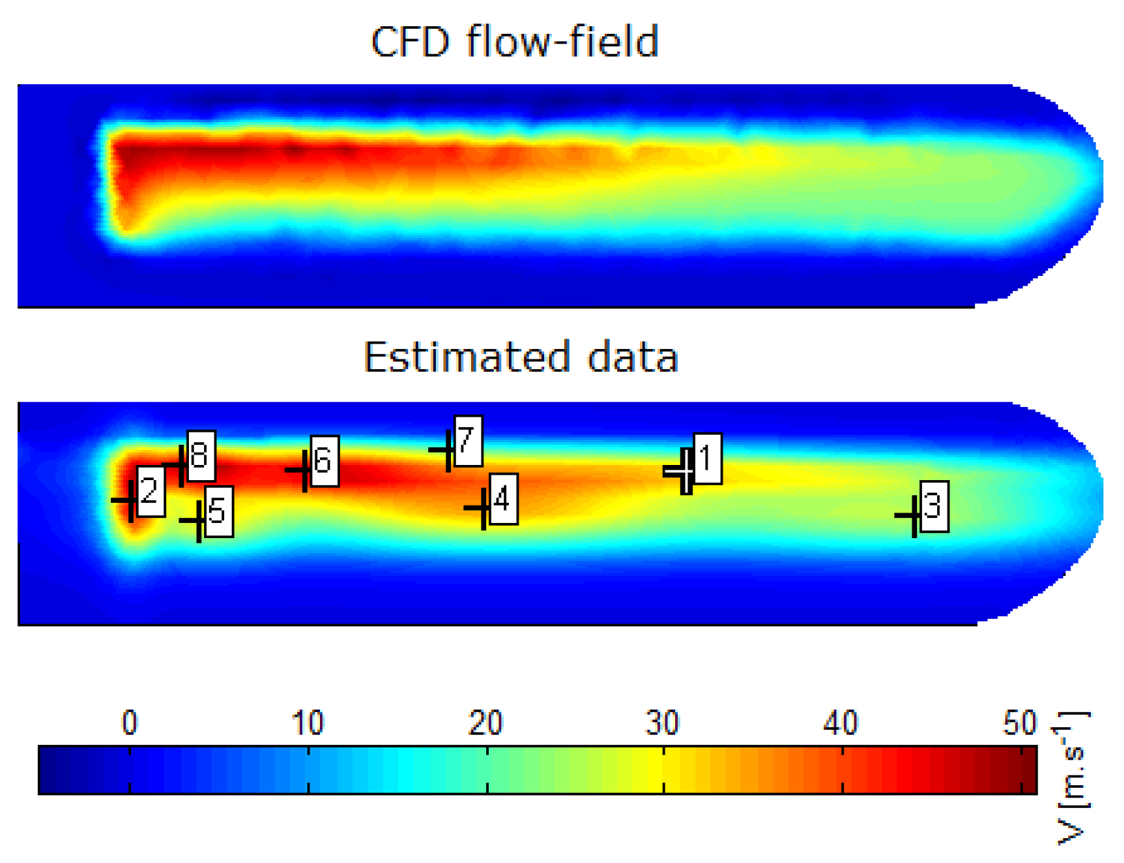
The Gaussian itself is defined by the five parameters , and is related to the spatial distribution of the velocity profile. The character of the oscillations is described by the sine function, specified by an additional three parameters with obvious physical meanings (oscillation frequency f, phase shift , and mean value ). The comparison between the calculated and approximate velocity at the nozzle exit is depicted in Figure 8. The numbered signs depict the locations of the Gaussians. The difference between the CFD and the approximated data was very small and could be neglected at this stage.
The velocity distribution from the CFD simulations, for various peak outlet velocities of the SaOB actuator, are shown in Figure 9. It shows how the values of maximum outlet velocities were extracted for the evaluation, as in Figure 5. It can also be seen that the shape of the velocity profile was essentially independent of the particular case (i.e., inlet pressure to the SaOB actuator), and that the velocity profiles are reasonably self-similar.
An optimization procedure was defined to obtain parameters that provided a minimum value of the cost function. Two parts of the cost function were defined to fulfill the desired characteristics of time dependent flow-field (see Figure 10) and total volume flow rate through the actuator. Therefore, the cost function is defined as:
where and are estimated and computed flow-field variables (velocities), respectively; and are estimated and computed volume flow rates, respectively; k is the number of samples (time instances); a and b are optimization weights; and is a design vector describing the flow variable, as in Equation (1). In this case, only eight steps () were used, which we considered sufficient, given the harmonic nature of the oscillations. The coefficient of determination = 99.15% for the mass flow evolution fit between the CFD data and the analytical function, which suggests that the process was described with sufficient accuracy.
Three different oscillation frequencies, across the entire range tested during the bench-top test, were calculated by this boundary condition for verification purposes. The courses of the volume flow rate, based on the vertical component of the blowing velocity, dependent on time, are depicted in Figure 10. The solid lines show the volume flow computed by the CFD, and the dashed lines are based on the prescribed values of the boundary condition. It was found that this functional representation enables the use of several parameters, common for the particular SaOB actuator, and only a few (the frequency f, and the amplitudes ) needed to be adjusted. Moreover, a linear dependence between the frequency and amplitudes was observed for this range of operational states (i.e., when the frequency of the oscillations is altered, only the amplitudes needed to be uniformly scaled). This scaling had to be determined, based on the evaluation of a range of cases.
4. Application to Circulation Control
The boundary condition with variable velocity profiles, as defined in Section 3, was applied to the low-speed airfoil, AR2, with the wind tunnel conditions according to [21]. Both possible regimes of the SaOB actuator were evaluated, namely full (including both suction and oscillatory blowing parts) and without suction (only oscillatory blowing). The experimental data were used for comparison with the CFD results presented here.
The computational domain consisted of one spanwise segment of the airfoil, incorporating only one pair of the SaOB outlet nozzles. The domain was set as periodic in the spanwise direction to simulate a row synchronized actuators, and it was extended to approximately 100 airfoil chords in the streamwise and normal directions. The suction was placed at 82% of the chord (on the upper surface of the airfoil) and the location of the blowing slots was at 95% of the chord (on the lower surface, near the trailing edge), see Figure 11.
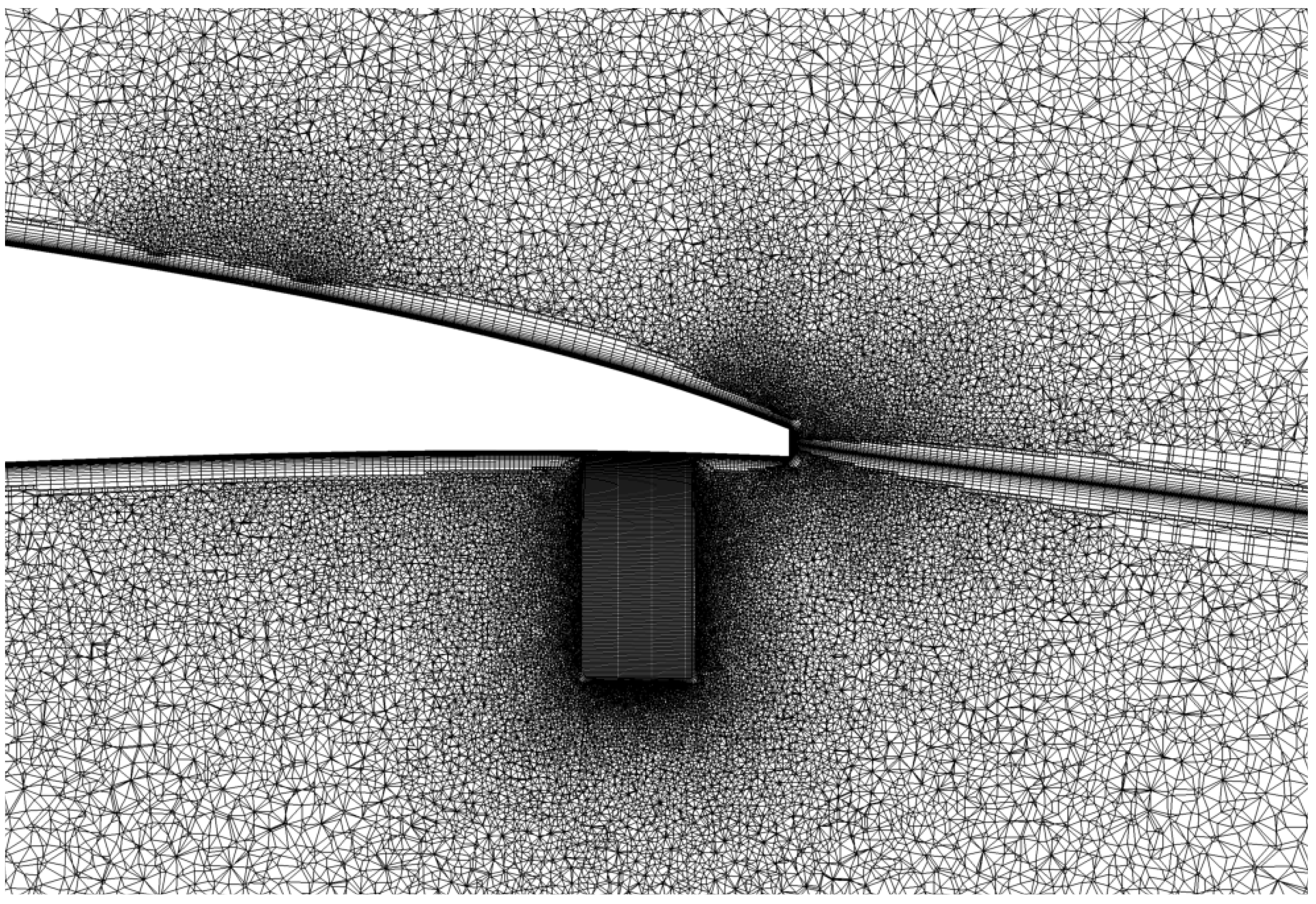
The computational grid had 5,978,534 nodes in total. The airfoil was resolved with approximately 800 points in the streamwise direction (around whole airfoil) with a fine resolution close to the leading edge, trailing edge, and near the positions of the suction and blowing slots. It was tuned to achieve the usual requirements for , with a Reynolds number of 600,000, based on the chord length and the freestream velocity m/s. Figure 12 shows the spanwise cut through the grid in the area of the trailing edge in detail.
4.1. CFD Simulations with the SaOB Boundary Condition
For the simulation of the effect of the oscillatory blowing part of the SaOB actuator, the velocity profile (defined by Equation (1)) was applied at the blowing slots, see Figure 11 (cyan). For the effect of the full SaOB, the additional surface boundaries for suction were added into the computational grid on the upper surface of the airfoil, see Figure 11 (green). The boundary conditions used at these suction holes prescribed mass flow, according to [31]. The parameters defined by Equation (1) were varied, to obtain the blowing velocity and oscillation frequency over the whole range of considered supply pressures used during the verification process.
The momentum coefficient was calculated, according to the equation:
where the area of the SaOB outlet slot and the maximum outlet velocity are put into relation with the reference area of the airfoil and the freestream velocity . The cut in the plane, normal to the streamwise direction, is shown in Figure 13. The case of full SaOB at and of only the oscillatory blowing (i.e., with the suction ports inactive) are depicted. Small differences between the values are visible, namely a slightly higher suction peak on the upper surface of the airfoil (the color map is reversed) is visible, and the stagnation point moved.
4.2. CFD Results and Experimental Data Comparison
The effect of ACF on , relative to the baseline configuration without any AFC, was evaluated and compared with the experimental data for Angle of Attack (AoA) = [21,24], see Figure 14.
The values of from the CFD simulations were in a good agreement with the experimental data. Although some differences still persisted, especially in the lower range of . These differences could be explained by small suction rates, where a small change could cause a relatively high effect.
The case of oscillatory blowing without added suction was simulated simply by switching the outflow boundary condition off and assigning the adiabatic wall boundary condition to the area of the suction ports. Figure 15 shows the integral values of , in relation to the .
It is possible to see that was slightly underestimated between the minimum and maximum values of the considered range; however, the trend was very similar. It has to be mentioned that the differences between measured and calculated values were within . This difference could be the result of the different experimental and CFD calibrations. In CFD, the was given by setting the oscillatory blowing boundary condition, while, in the experiment, was correlated with supply pressure. Suction through the openings was considered during the bench-top test calibration. The suction flow increased the mass flow rate through the actuator’s outlets, which resulted in the slightly higher blowing velocity—and, hence, a higher .
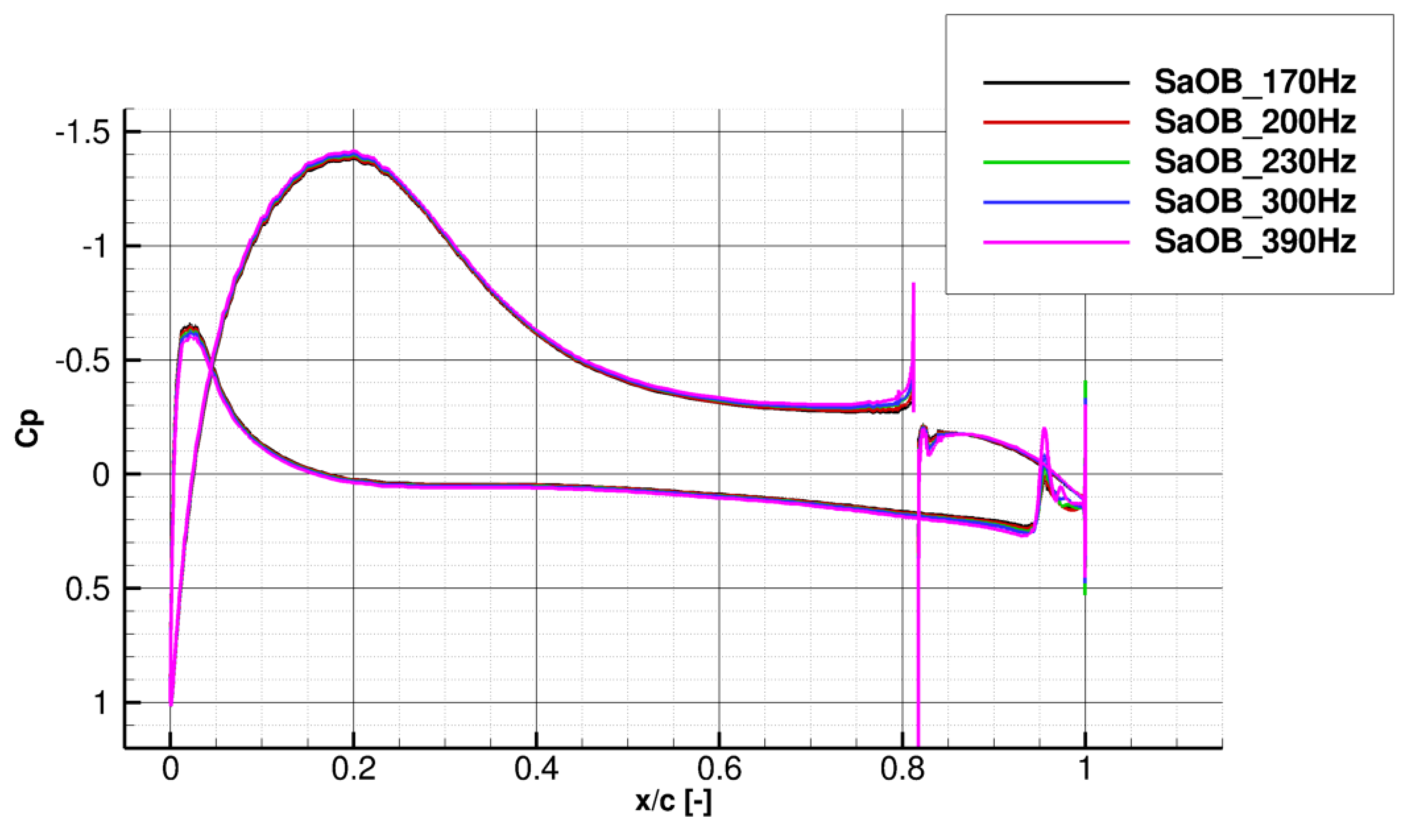
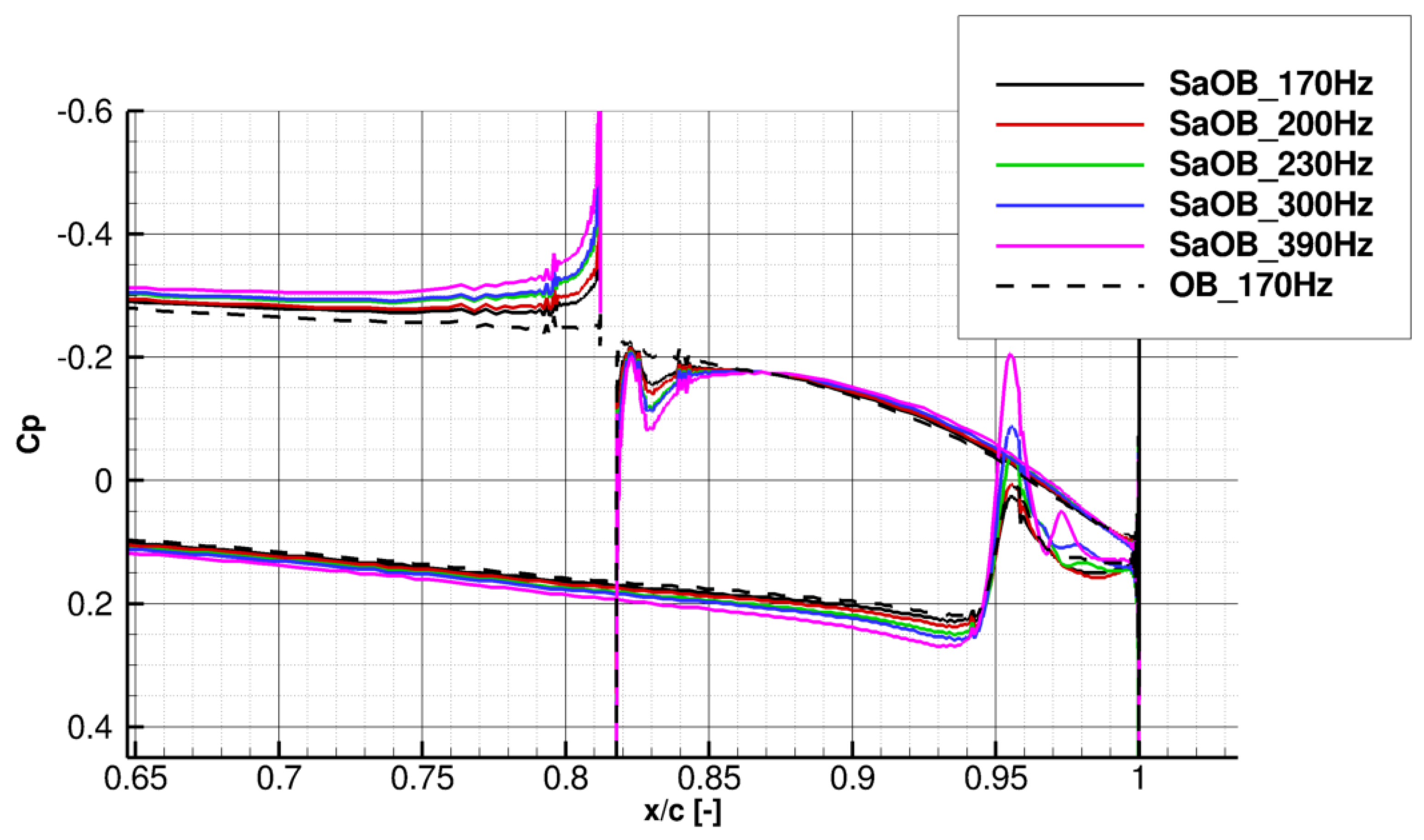
The local distribution provides another way to assess the results. As was already seen in Figure 13, small differences can be expected. Figure 16 shows the systematic change of due to suction (on the upper side of the airfoil), and also upstream of the oscillatory blowing (on the lower side of the airfoil). The oscillation frequency was used to denote specific cases; however, the maximum blowing velocity changes accordingly, as well. The detail of the trailing edge region distribution is shown in Figure 17, where both the SaOB and oscillatory blowing are visible. It can be seen that the effect of oscillatory blowing (without suction) was limited mostly to the variation on the lower side of the airfoil, upstream of the oscillatory blowing slots. This explains why the effect of SaOB was significantly higher, see Figure 14 and Figure 15. This also shows how important it is to carefully select the positioning of the AFC devices.
5. Conclusions
The time-dependent simplified boundary condition of the SaOB, based on the URANS simulations of the actuator’s internal flowfield in still-air ambient conditions, has been defined. The developed boundary condition has been implemented into the CFD code, and verified for different blowing velocities and oscillation frequencies in the case of a low-speed airfoil, where steady suction and oscillatory blowing were applied at the upper and lower surfaces, respectively. Both cases have been simulated and validated against the experimental data. The obtained results are in a very good agreement with the experimental data; nevertheless, some differences in still exist, especially in the case of pure oscillatory blowing without suction. These differences in could be related to the calibration of both (experimental and CFD) methods. While the experimental data relate the blowing velocity to the supply pressure into the SaOB actuator, calibrated in still-air conditions, the CFD directly prescribes velocity components at the actuator boundary condition.
Although the simulations still need to be run in unsteady mode with a sufficiently small time step, applying this simplified boundary condition will allow for a reduction in grid points, by omitting the complex internal geometry of the actuator and, hence, save computational resources and time.
This simplified boundary condition will also enable efficient simulations of actuator arrays, used in low-speed as well as high-speed engineering applications, and will make the direct application of the AFC to the design process more feasible. Our follow-up work will be focused on the use of the presented boundary condition on additional typical aerodynamic applications, as in the case of separation control of the high-lift configuration with an ultra-high bypass ratio engine—the primary goal of the project under which the work has been performed.
Author Contributions
P.V. defined the problem, performed the calculations, extracted and analyzed the data, and provided parts of the manuscript. P.H. established the functional representation and provided parameters for the boundary condition definition. A.P. implemented the code, performed part of the calculations, analyzed the data, and finalized the manuscript.
Funding
The work presented in this paper and the research leading to these results has received funding from the European Commission under the Clean Sky 2 programme H2020-EU.3.4.5.1.—IADP Large Passenger Aircraft, grant agreement ID 754307, INAFLOWT project.
Acknowledgments
This work also was supported by The Ministry of Education, Youth, and Sports of the Czech Republic from the Large Infrastructures for Research, Experimental Development, and Innovations project IT4Innovations National Supercomputing Center LM2015070. Furthermore, the authors wish to thank our colleague Miroslav Šmíd for providing computational grids, and to Avraham Seifert and Danny Dolgopyat, who provided the experimental data.
Conflicts of Interest
The authors declare no conflict of interest.
Abbreviations
The following abbreviations are used in this manuscript:
| AFC | Active Flow Control |
| AoA | Angle of Attack |
| CFD | Computational Fluid Dynamics |
| CPU | Central Processing Unit |
| Jet momentum coefficient, | |
| DDES | Delayed Detached Eddy Simulation |
| f | frequency (Hz) |
| LES | Large Eddy Simulation |
| PIV | Particle Image Velocimetry |
| RANS | Reynolds Average Navier–Stokes |
| SST | Menter’s Shear Stress Transport (turbulence model) |
| Reference area | |
| Outlet slot area | |
| t | Time (s) |
| Maximum jet velocity (m/s) | |
| Free stream velocity (m/s) | |
| URANS | Unsteady Reynolds Average Navier–Stokes |
| Maximum velocity from the SaoB actuator nozzle (m/s) |
References
- Blaylock, M.; Chow, R.; Cooperman, A.; van Dam, C.P. Comparison of pneumatic jets and tabs for Active Aerodynamic Load Control. Wind Energy 2014, 17, 1368–1384. [Google Scholar] [CrossRef]
- Rumsey, C. Successes and Challenges for Flow Control Simulations (Invited). In Proceedings of the 4th Flow Control Conference, Fluid Dynamics and Co-located Conferences, AIAA 2008-4311, Seattle, WA, USA, 23–26 June 2008. [Google Scholar] [CrossRef]
- Lengers, M. Industrial assessment of overall aircraft driven local active flow control. In Proceedings of the 29th Congress of the International Council of the Aeronautical Sciences, St. Petersburg, Russia, 7–12 September 2014. [Google Scholar]
- Seifert, A.; Shtendel, T.; Dolgopyat, D. From lab to full scale Active Flow Control drag reduction: How to bridge the gap? J. Wind Eng. Ind. Aerodyn. 2015, 147, 262–272. [Google Scholar] [CrossRef]
- Morgulis, N.; Seifert, A. Fluidic flow control applied for improved performance of Darrieus wind turbines. Wind Energy 2016, 19, 1585–1602. [Google Scholar] [CrossRef]
- Vrchota, P.; Hospodář, P. Response Surface Method Application to High-Lift Configuration with Active Flow Control. J. Aircr. 2012, 49, 1796–1802. [Google Scholar] [CrossRef]
- Galbraith, M. Numerical Simulations of a High-Lift Airfoil Employing Active Flow Control. In Proceedings of the 44th AIAA Aerospace Sciences Meeting, Reno, Nevada, 9–12 January 2006. [Google Scholar] [CrossRef]
- Yousefi, K.; Saleh, R. Three-dimensional suction flow control and suction jet length optimization of NACA 0012 wing. Meccanica 2015, 50, 1481–1494. [Google Scholar] [CrossRef] [Green Version]
- Huang, L.; Huang, P.G.; LeBeau, R.P.; Hauser, T. Numerical Study of Blowing and Suction Control Mechanism on NACA0012 Airfoil. J. Aircr. 2004, 41, 1005–1013. [Google Scholar] [CrossRef]
- Yousefi, K.; Saleh, R. The Effects of Trailing Edge Blowing on Aerodynamic Characteristics of the NACA 0012 Airfoil and Optimization of the Blowing Slot Geometry. J. Theor. Appl. Mech. 2014, 52, 165–179. [Google Scholar] [CrossRef]
- Rumsey, C.L.; Nishino, T. Numerical study comparing RANS and LES approaches on a circulation control airfoil. Int. J. Heat Fluid Flow 2011, 32, 847–864. [Google Scholar] [CrossRef] [Green Version]
- Schatzman, D.M.; Wilson, J.; Maron, L.; Palei, V.; Seifert, A.; Arad, E. Suction and oscillatory blowing interaction with boundary layers. In Proceedings of the 53rd AIAA Aerospace Sciences Meeting, AIAA SciTech Forum, Kissimmee, FL, USA, 5–9 January 2015. [Google Scholar]
- Lakebrink, M.T.; Mani, M.; Winkler, C. Numerical Investigation of Fluidic Oscillator Flow Control in an S-Duct Diffuser. In Proceedings of the 55th AIAA Aerospace Sciences Meeting, Grapevine, TX, USA, 9–13 January 2017. [Google Scholar]
- Vrchota, P. Active Flow Separation Control Applied at Wing-Pylon Junction of a Wing Section in Landing Configuration. In Proceedings of the 55th AIAA Aerospace Sciences Meeting, Grapevine, TX, USA, 9–13 January 2017; p. 0491. [Google Scholar]
- Vatsa, V.; Koklu, M.; Wygnanski, I. Numerical Simulation of Fluidic Actuators for Flow Control Applications. In Proceedings of the 6th Flow Control Conference, Fluid Dynamics and Co-located Conferences, New Orleans, LA, USA, 25–28 June 2012. AIAA 2012-3239. [Google Scholar] [CrossRef]
- Kara, K. Numerical Study of Internal Flow Structures in a Sweeping Jet Actuator. In Proceedings of the 33rd AIAA Applied Aerodynamics Conference, Atlanta, GA, USA, 16–20 June 2015. AIAA 2015-2424. [Google Scholar]
- Troshin, V.; Palei, V.; Shtendel, T.; Seifert, A. Characterization of the Suction and Oscillatory Blowing Actuator in Still Air. In Proceedings of the 54th Israel Annual Conference on Aerospace Sciences, Tel Aviv, Israel, 19–20 February 2014. [Google Scholar]
- Arwatz, G.; Fono, I.; Seifert, A. Suction and oscillatory blowing actuator modeling and validation. AIAA J. 2008, 46, 1107–1117. [Google Scholar] [CrossRef]
- Wallin, S.; Johansson, A.V. An explicit algebraic Reynolds stress model for incompressible and compressible turbulent flows. J. Fluid Mech. 2000, 403, 89–132. [Google Scholar] [CrossRef]
- Gritskevich, M.S.; Garbaruk, A.V.; Schütze, J.; Menter, F.R. Development of DDES and IDDES Formulations for the k–ω Shear Stress Transport Model. Flow Turbul. Combust. 2012, 88, 431–449. [Google Scholar] [CrossRef]
- Dolgopyat, D.; Seifert, A. Active Flow Control Virtual Maneuvering System Applied to Conventional Airfoil. AIAA J. 2019, 57, 72–89. [Google Scholar] [CrossRef]
- Kim, J.; Moin, P.; Seifert, A. Large-Eddy Simulation-Based Characterization of Suction and Oscillatory Blowing Fluidic Actuator. AIAA J. 2017, 55, 2566–2579. [Google Scholar] [CrossRef]
- Vrchota, P.; Prachař, A.; Hospodář, P.; Dolgopyat, D.; Seifert, A. Development and Verification of Simplified Boundary Condition of SaOB Actuator. In Proceedings of the 58th Israel Annual Conference on Aerospace Sciences, Tel Aviv, Israel, 14–15 March 2018. [Google Scholar]
- Dolgopyat, D.; Seifert, A. Conventional Airfoil Active Flow Control Virtual Maneuvering System. In Proceedings of the 55th Israel Annual Conference on Aerospace Sciences, Tel Aviv, Israel, 25–26 February 2015. [Google Scholar]
- Vrchota, P.; Prachař, A.; Hospodář, P.; Dolgopyat, D.; Seifert, A. Development of Simplified Boundary Condition of SaOB Actuator Based on High-Fidelity CFD Simulations. In Proceedings of the 52nd 3AF International Conference on Applied Aerodynamics—Progress in Flow Control, Lyon, France, 27–29 March 2017. [Google Scholar]
- Prachař, A.; Vrchota, P. Characterization of the Suction-and-Oscillatory-Blowing actuator by the hybrid RANS-LES CFD. In Proceedings of the 2018 Flow Control Conference, AIAA AVIATION Forum, Atlanta, GA, USA, 25–29 June 2018. [Google Scholar] [CrossRef]
- Eliasson, P. EDGE, a Navier-Stokes Solver for Unstructured Grid; ISTE Ltd.: London, UK, 2002; pp. 527–534. [Google Scholar]
- Swanson, R.C.; Radespiel, R.; Turkel, E. On Some Numerical Dissipation Schemes. J. Comput. Phys. 1998, 147, 518–544. [Google Scholar] [CrossRef] [Green Version]
- Zhang, X.S. Neural Networks in Optimization; Springer Science & Business Media: Berlin/Heidelberg, Germany, 2013; Volume 46. [Google Scholar]
- Rasmussen, C.E.; Williams, C.K.I. Gaussian Processes for Machine Learning (Adaptive Computation and Machine Learning); The MIT Press: Cambridge, MA, USA, 2005. [Google Scholar]
- Jirasek, A. Mass flow boundary conditions for subsonic inflow and outflow boundary. AIAA J. 2006, 44, 939–947. [Google Scholar] [CrossRef]
Figure 1.
Schematic rendering of the Suction and Oscillatory Blowing (SaOB) actuator: (a) Ejector, and (b) switching valve (adopted from [18]).
Figure 1.
Schematic rendering of the Suction and Oscillatory Blowing (SaOB) actuator: (a) Ejector, and (b) switching valve (adopted from [18]).

Figure 2.
The geometry of the SaOB actuator; the shade color represents the adiabatic wall boundary conditions.
Figure 2.
The geometry of the SaOB actuator; the shade color represents the adiabatic wall boundary conditions.

Figure 3.
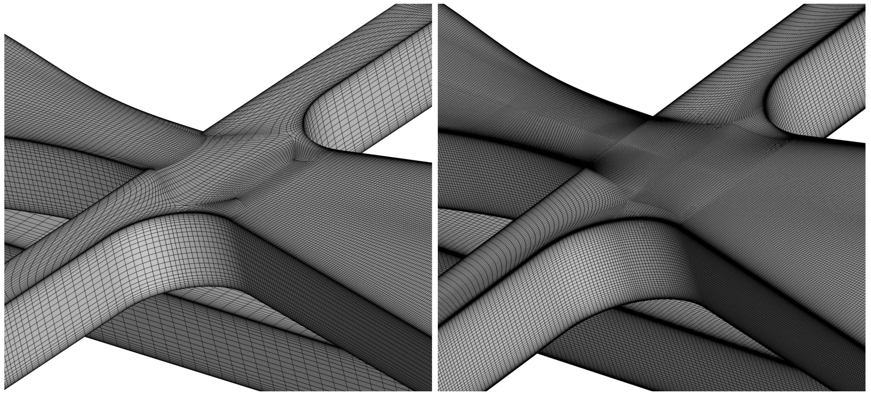
Detail of the surface computational grids for the URANS calculations with 5.5 million grid points (left) and for the hybrid SST-DDES (right), refined to nearly 21 million grid points in total, with 12 million inside the actuator. See Table 1 for details.
Figure 3.
Detail of the surface computational grids for the URANS calculations with 5.5 million grid points (left) and for the hybrid SST-DDES (right), refined to nearly 21 million grid points in total, with 12 million inside the actuator. See Table 1 for details.

Figure 4.
Snapshot of typical flow inside the SaOB actuator. The main areas, with respect to the character of the flow, are highlighted, adopted from [26].
Figure 4.
Snapshot of typical flow inside the SaOB actuator. The main areas, with respect to the character of the flow, are highlighted, adopted from [26].

Figure 5.
Comparison of the Computational Fluid Dynamics (CFD) results with the experimental data [21].
Figure 5.
Comparison of the Computational Fluid Dynamics (CFD) results with the experimental data [21].

Figure 6.
Normalized velocity at the actuator exit at the peak velocity phase (left nozzle), adopted from [26].
Figure 6.
Normalized velocity at the actuator exit at the peak velocity phase (left nozzle), adopted from [26].

Figure 7.
Comparison of exit velocity profile, normalized by the maximum velocity. The URANS results (dashed) and SST-DDES simulations (solid) are shown. Green lines represent the peak velocity snapshot for the left outlet nozzle, and red lines represent peak velocity for the right nozzle.
Figure 7.
Comparison of exit velocity profile, normalized by the maximum velocity. The URANS results (dashed) and SST-DDES simulations (solid) are shown. Green lines represent the peak velocity snapshot for the left outlet nozzle, and red lines represent peak velocity for the right nozzle.

Figure 8.
Comparison of the calculated and approximated vertical velocity components, corresponding to the same time instant. A snapshot of the CFD flowfield (top) is compared to the approximation using Gaussians (bottom). The numbered marks represent the coordinates , as in Equation (1).
Figure 8.
Comparison of the calculated and approximated vertical velocity components, corresponding to the same time instant. A snapshot of the CFD flowfield (top) is compared to the approximation using Gaussians (bottom). The numbered marks represent the coordinates , as in Equation (1).

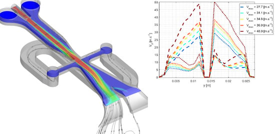
Figure 9.
Determination of the peak velocity from the surface interpolation of the velocity field at the nozzle exits. The left figure displays velocity profiles at the peak velocity time instant in the right and the left outlet nozzles of the SaOB actuator, respectively. The dashed and dotted black lines show a spanwise cut through the maximum velocity location. The graph on the right displays velocity profiles at the peak velocities of (approximately) 28 m/s, 31 m/s, 35 m/s, 37 m/s, and 49 m/s (colors are according to line legend). The dashed lines represent velocity peaks at the left nozzle, dotted lines are the right nozzle peaks.

Figure 10.
Volume flow rates—calculated and prescribed by the boundary condition model—for three different SaOB working states.
Figure 10.
Volume flow rates—calculated and prescribed by the boundary condition model—for three different SaOB working states.

Figure 11.
Detail of the CFD surface grid around trailing edge of the AR2 airfoil. The cyan surface represents blowing slots, the green color marks the circular suction holes.
Figure 11.
Detail of the CFD surface grid around trailing edge of the AR2 airfoil. The cyan surface represents blowing slots, the green color marks the circular suction holes.

Figure 12.
Detail of the spanwise cut through the CFD grid close to the trailing edge of the AR2 airfoil. A structured block, to resolve oscillatory blowing and the wake, is included.
Figure 12.
Detail of the spanwise cut through the CFD grid close to the trailing edge of the AR2 airfoil. A structured block, to resolve oscillatory blowing and the wake, is included.

Figure 13.
Comparison of full suction and oscillatory blowing (top) and plain oscillatory blowing (bottom) cases. Both simulations were run with an oscillation frequency of 300 Hz, and Angle of Attack (AoA) = 0°.
Figure 13.
Comparison of full suction and oscillatory blowing (top) and plain oscillatory blowing (bottom) cases. Both simulations were run with an oscillation frequency of 300 Hz, and Angle of Attack (AoA) = 0°.

Figure 14.
Comparison of the experimental data (taken from [21]) with the CFD results. Steady suction and oscillatory blowing actuator active.
Figure 14.
Comparison of the experimental data (taken from [21]) with the CFD results. Steady suction and oscillatory blowing actuator active.

Figure 15.
Comparison of the experimental data (see [21]), and the CFD results. Oscillatory blowing without suction. Black lines represent trend.
Figure 15.
Comparison of the experimental data (see [21]), and the CFD results. Oscillatory blowing without suction. Black lines represent trend.
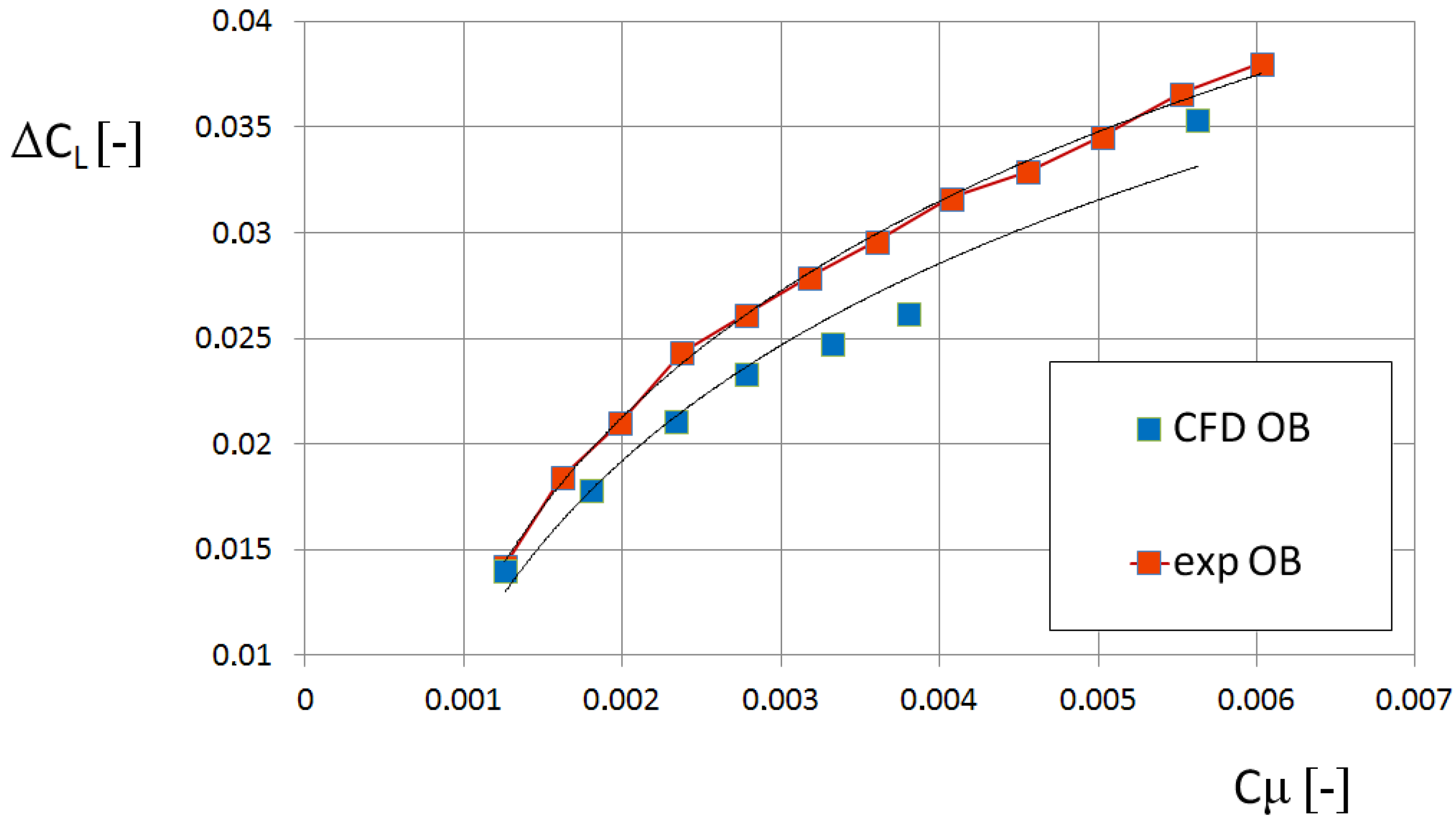
Figure 16.
distribution of the SaOB cases.

Figure 17.
Detail of distribution at the trailing edge region. SaOB case (top) and oscillatory blowing (bottom). Oscillatory blowing for low is added to the upper figure, for reference.
Figure 17.
Detail of distribution at the trailing edge region. SaOB case (top) and oscillatory blowing (bottom). Oscillatory blowing for low is added to the upper figure, for reference.


Table 1.
Grid parameters for the URANS and SST-DDES grid cases.
| Grid Part | URANS Grid | SST-DDES Grid | ||
|---|---|---|---|---|
| # Points | First Cell (mm) | # Points | First Cell (mm) | |
| Total | 5,418,072 | – | 20,770,098 | – |
| Feedback tube | 398,033 | 0.01 | 3,882,487 | 0.003 |
| Nozzle and outputs | 2,668,014 | 0.01–0.001 | 7,819,016 | 0.008–0.001 |
© 2019 by the authors. Licensee MDPI, Basel, Switzerland. This article is an open access article distributed under the terms and conditions of the Creative Commons Attribution (CC BY) license (http://creativecommons.org/licenses/by/4.0/).
Share and Cite
MDPI and ACS Style
Vrchota, P.; Prachař, A.; Hospodář, P. Verification of Boundary Conditions Applied to Active Flow Circulation Control. Aerospace 2019, 6, 34. https://doi.org/10.3390/aerospace6030034
AMA Style
Vrchota P, Prachař A, Hospodář P. Verification of Boundary Conditions Applied to Active Flow Circulation Control. Aerospace. 2019; 6(3):34. https://doi.org/10.3390/aerospace6030034
Chicago/Turabian StyleVrchota, Petr, Aleš Prachař, and Pavel Hospodář. 2019. "Verification of Boundary Conditions Applied to Active Flow Circulation Control" Aerospace 6, no. 3: 34. https://doi.org/10.3390/aerospace6030034
Note that from the first issue of 2016, this journal uses article numbers instead of page numbers. See further details here.