Technical Note

Correlated Bayesian Model of Aircraft Encounters in the Terminal Area Given a Straight Takeoff or Landing

Massachusetts Institute of Technology, Lincoln Laboratory, Lexington, MA 02421, USA
*
Author to whom correspondence should be addressed.
Aerospace 2022, 9(2), 58; https://doi.org/10.3390/aerospace9020058
Submission received: 1 November 2021 / Revised: 13 January 2022 / Accepted: 18 January 2022 / Published: 24 January 2022
(This article belongs to the Collection Air Transportation—Operations and Management)

Abstract

:
The integration of new airspace entrants into terminal operations requires design and evaluation of Detect and Avoid systems that prevent loss of well clear from and collision with other aircraft. Prior to standardization or deployment, an analysis of the safety performance of those systems is required. This type of analysis has typically been conducted by Monte Carlo simulation with synthetic, statistically representative encounters between aircraft drawn from an appropriate encounter model. While existing encounter models include terminal airspace classes, none explicitly represents the structure expected while engaged in terminal operations, e.g., aircraft in a traffic pattern. The work described herein is an initial model of such operations where an aircraft landing or taking off via a straight trajectory encounters another aircraft landing or taking off, or transiting by any means. The model shares the Bayesian network foundation of other Massachusetts Institute of Technology Lincoln Laboratory encounter models but tailors those networks to address structured terminal operations, i.e., correlations between trajectories and the airfield and each other. This initial model release is intended to elicit feedback from the standards-writing community.

1. Introduction

The National Airspace System (NAS) is a complex and evolving system that enables safe and efficient aviation. New airspace entrants are leveraging the NAS in new, novel, and different ways than traditional aviation with a pilot onboard. To enable growth in the industry, expansion of applications, and new economic opportunities, new entrants must integrate into the NAS without degrading overall safety or efficiency of the existing operations. To help achieve this, standards developing organizations, such as ASTM International and RTCA, have established and continue to update performance-based standards for Detect and Avoid (DAA) systems.
DAA systems are designed as an electronic means of compliance to the primarily visual-based separation responsibilities of a pilot and to comply with applicable operating rules of Title 14 of the Code of Federal Regulations (14 CFR). Some of these rules include 14 CFR §91.3, 91.111, 91.113(b), 91.115, 91.123, and 91.181(b) [1], which prescribe that aircraft must not operate carelessly or recklessly; not operate so close to another aircraft so as to create a collision hazard, see and avoid other aircraft, and give way to other aircraft that have the right of way.
DAA is part of a multi-layered airspace conflict management architecture and DAA is often not employed until prior strategic mitigations have failed [2]. While there is a singular standard for crewed aircraft collision avoidance, there are a variety of DAA standards that are primarily organized by size of the aircraft; expected operations by airspace class or altitude; and how prescriptive the standard is written.
A foundational element to these standards is modeling and simulation activities to design and evaluate the safety and suitability of a DAA system. Monte Carlo simulations in particular enable surveillance systems and algorithms to be tested under an exhaustive set of circumstances not possible through live flight testing. The simulations are often validated through human-in-the-loop experiments and flight testing. For example, an update to the standard prescribing a collision avoidance system for crewed aircraft was validated in part using this approach [3].

1.1. Motivation

As part of the modeling and simulation activities, the Massachusetts Institute of Technology Lincoln Laboratory (MIT LL) statistical encounter models have been used to model aircraft behavior. These are trained on real-world observations of individual aircraft or observations of encounters between two aircraft. The majority of these models are uncorrelated [4,5,6,7], which assume that the aircraft are not participating in the air traffic control system and their behavior is independent of other aircraft. Conversely, a correlated model assumes that aircraft behavior and the relatively geometry between aircraft was dependent upon an air traffic service. For example, air traffic control will separate aircraft to minimize the possible effects of wake turbulence. While wake turbulence is not explicitly modeled, a correlated model will be trained using aircraft tracks that have been separated by air traffic control to minimize the wake turbulence risk. Currently [8], sampling a correlated model generates track information for two aircraft while sampling an uncorrelated model generates independent track information for one aircraft.
While MIT LL previously developed [9] and updated [10] an en route correlated model, it was designed to model encounters that occur away from airports in terminal airspaces, or while one or both aircraft are merely passing through the terminal airspace. This en route model does not represent the standardized approach and departure routes that describe the permissible flight paths for large airports, or smaller airports employing a standardized flight pattern to regulates flow into and out of the airport. The lack of a model tailored to terminal operation is a capability gap identified by the aviation standards developing organization, RTCA, Special Committee (SC)-228 developing a variety of aviation performance standards, including DAA standards being developed in multiple phases [11]. Other standards efforts by RTCA SC-147 and ASTM F38 have also expressed interested in a terminal airspace model, particularly for metropolitan areas.
Specifically, RTCA SC-228 and the FAA have requested the model development to support modeling and simulation related to DAA Minimum Operating Performance Standards (MOPS), DO-365. Revision A of DO-365 was previously validated primarily in simulation [12]; and published as revision A [1]. Revision B was published in 2021, addressing some terminal operations that were out of scope for revision A.

1.2. Scope

The model development scope was directly informed by the terms of reference of RTCA SC-228 [11], specifically those associated with DO-365 revision B. Considered were geographically limited operations and operations within a terminal environment, which include Class D airspace, towered airfields within Class E airspace, non-towered airfields within Class E airspace, non-towered airfields within Class G airspace, takeoff and landing operations in Class C, D, E, and G airspace, and off-airfield launch and recovery sites within Class G airspace. Notably, operations in Class B airspace, which generally are the most complex and busiest, and 14 CFR Part 135 cargo operations were out of scope per the RTCA SC-228 terms of reference.
RTCA SC-228 defined the terminal environment as within 8 nautical miles laterally and 3000 feet vertically of a runway. We adopted a slightly larger definition of 8 nautical miles laterally and 5000 vertically of a runway. We defined an encounter as when two aircraft are within 4 nautical miles laterally and 2000 feet vertically of each other for at least one second. Aircraft must overlap in time for at least thirty seconds too. To manage model complexity, we only considered encounters with exactly two aircraft and assumed at least one aircraft lands via a straight-in approach or an analogous departure route.

1.3. Objectives and Contributions

The primary objective is to develop a statistical model that represents aircraft behavior in the terminal environment and then sample this model to create an encounter set to support safety analyses. Since terminal airspaces can be traffic dense, the developed model needs to be cognizant of the airspace structure that provides implicit coordination and communicates intent amongst all the airspace users. Although every airport is different and traffic patterns likewise vary, assessing encounters specific to the traffic at one airport is not sufficient to deem a DAA system safe for terminal operations at all airports. Traffic patterns may be tailored to account for various configurations of runways as well as external factors like surrounding terrain or other natural or human-made features
Accordingly, the primary contribution was a set of Dynamic Bayesian models representative of single-runway airports in Class C, D, or E/G airspace and potentially representative of Class B. These models characterized the interaction between two aircraft. One aircraft must be either on a straight-in approach or straight-out departure while the other can approach or depart without restrictions, along with simply transiting through the airspace. Similar to other recently developed models [13], this terminal model considered the type of aircraft (e.g., fixed-wing and rotorcraft). Discussion of our materials and methods is described in sufficient detail to allow others to replicate and build on the contributions.
The primary contribution was preceded by an initial prototype model (version 1.0) narrowly scoped to aircraft on straight-in approach to a Class D single-runway airport encountering a second aircraft either landing or taking off; and a subsequent prototype (version 2.0) that added Class E/G single-runway airports, straight-out departures, and transiting aircraft. A dataset of sampled encounters using the version 1.0 was publicly released, but the Bayesian models for the two prototypes were not made publicly available. Only version 3.0 was released as open source software in July 2021 [14], with software to sample the models first released in October 2021 [8].
As of January 2021, the primary objective has not been fully and model development of the terminal or metropolitan environments are ongoing.

2. Materials and Methods

This section briefly overviews the training datasets, assumptions, prior art, and method to train a statistical model based on classified aircraft tracks.

2.1. Materials and Datasets

Two sets of data were used to train two separate encounter models: (1) FAA collected terminal radar track data over the period January through September 2015 at select airports throughout the NAS and (2) 190+ days of data over the period January 2019 through February 2020 from the OpenSky Network, a database consisting of ADS-B and Mode S reports [15]. The first is referred to as the “terminal area radar” dataset while the ADS-B dataset is referred to as the “aerodromes” dataset because the dataset is based on observations of aircraft in near airports in Class B, C, and D airspaces across the United States. Notably, the aerodromes dataset differed from the Mondays dataset, another curated from the OpenSky Network to train the recent uncorrelated encounter models [16].
These two sources of data have different assumptions and surveilled different types of aircraft. Training multiple models enabled us to assess the sensitivity of the models to different biases, while mitigating some weakness for a given dataset. Biases include the type of aircraft observed, the metadata associated with each surveilled track, or surveillance error. Data near fixed-runway airports in Class C, D, E, and G airspaces were in scope for version 3.0 of the model.
The terminal area radars data provided to MIT LL included standard aviation transponders with Mode A, C, and S capabilities. The OpenSky Network surveils aircraft only equipped with ADS-B, where ADS-B aircraft also generally support Mode C while not all Mode C aircraft are also equipped with ADS-B. However, the terminal area radars have a more limited spatial and temporal scope, whereas the OpenSky Network has better theoretical surveillance coverage. Additionally, the OpenSky Network was freely and easily available whereas the terminal area radar data were not.
Table 1 reports that each dataset had billions of interpolated observations of aircraft at altitudes below 5000 feet AGL, based on barometric altitude reports, and prior to any spatial filtering performed as part of model training. Appendix A discusses the datasets in more detail.

2.2. Assumptions

Encounters consist of two aircraft, with the first aircraft referred to as the ownship and the other aircraft referred to as the intruder. Many, not all, of our assumptions were derived from DO-365B. Important assumptions for developing and training the model included:
  • An encounter is when ownship and intruder are within 4 nautical miles laterally and 2000 feet vertically of each other for at least one second over at least a thirty second duration;
  • Ownship is on a straight-in takeoff or approach;
  • Intruder aircraft may be landing, taking off, or transiting the area;
  • Intruder aircraft may not be landing or taking off from a nearby airport;
  • Sampled trajectories are constrained to within 8 NM of the airfield and 5000 ft above airfield elevation (minimum altitude is 200 ft above airport elevation); and
  • Sampled trajectories are a maximum of 300 s in length.

2.3. Prior Art

The trained models align with the Bayesian network framework of other MIT LL encounter models [5] but are reformulated to account for the structured behavior aircraft employ when landing or taking off. Like the existing radar-based en route correlated encounter model [10], this terminal encounter model represents the relative geometry of two aircraft. While the other correlated model defined relative geometry based on the horizontal and vertical separation between aircraft, the geometry of this terminal encounter model was based on the relative geometry between each aircraft and the runway.
Notably, our approach also does not identify and model turning points, a concept popularized by Gariel et al. [17]. Mahboubi and Kochenderfer [18] demonstrated that a turning point model performs well on simulated data; due to its reliance on noisy heading rates, it has difficulty with real-world data. Our approach also differs from Barrett [19] et al. who used an unsupervised cluster algorithm to identify departure and approach procedures and fit the clusters to a generative model based on intra-cluster covariance matrices. Barrett [19] et al. was inspired by the clustering approach previous proposed by Li et al. [20,21]. Similar to these other efforts, we also do not leverage filed or amended flight plans like Krozel [22] or Georgiou et al. [23]. Additionally, we did not consider aircraft trajectories on the surface, such as Churchill and Bloem [24].

2.4. Methods Overview

Our approach clustered and classified tracks based on assumptions of airport design, approach and departure routes, and aviation heuristics, such as the 1 in 60 rule (one degree offset angle equates to one nautical mile displacement at 60 nautical miles from a origin). Additionally, we did not employ unsupervised learning techniques as we wanted to take advantage of known physical states during takeoff or landing operations. Namely, aircraft taking off or landing should have a low AGL altitude when close to the runway and that aircraft transiting over the airport would do so at higher altitudes. Consequently, our approach was computationally efficient, enabling us to train a model based on billions of observations. Furthermore, RTCA and ASTM committee members, the immediate users of the trained model, preferred for our newly trained model to be consistent with previous encounter models. Consequently, the model was trained using a similar Bayesian framework, and we did not explore training other types of models, such as a random forest model. Our approach consists of the following:
  • Download and pre-process (i.e., interpolate, outlier detection, etc.) training data;
  • Coarsely spatially filter training data to terminal airspace;
  • Classify track intent (e.g., landing, taking off, transiting) for training data within terminal airspace;
  • Given classified tracks, identify encounters between aircraft;
  • Train model using identified encounters;
  • Sample model to create representative encounters.

3. Track Filtering and Encounter Identification

This section discusses the filtering of tracks based on spatial and temporal conditions and how encounters between two aircraft were classified.

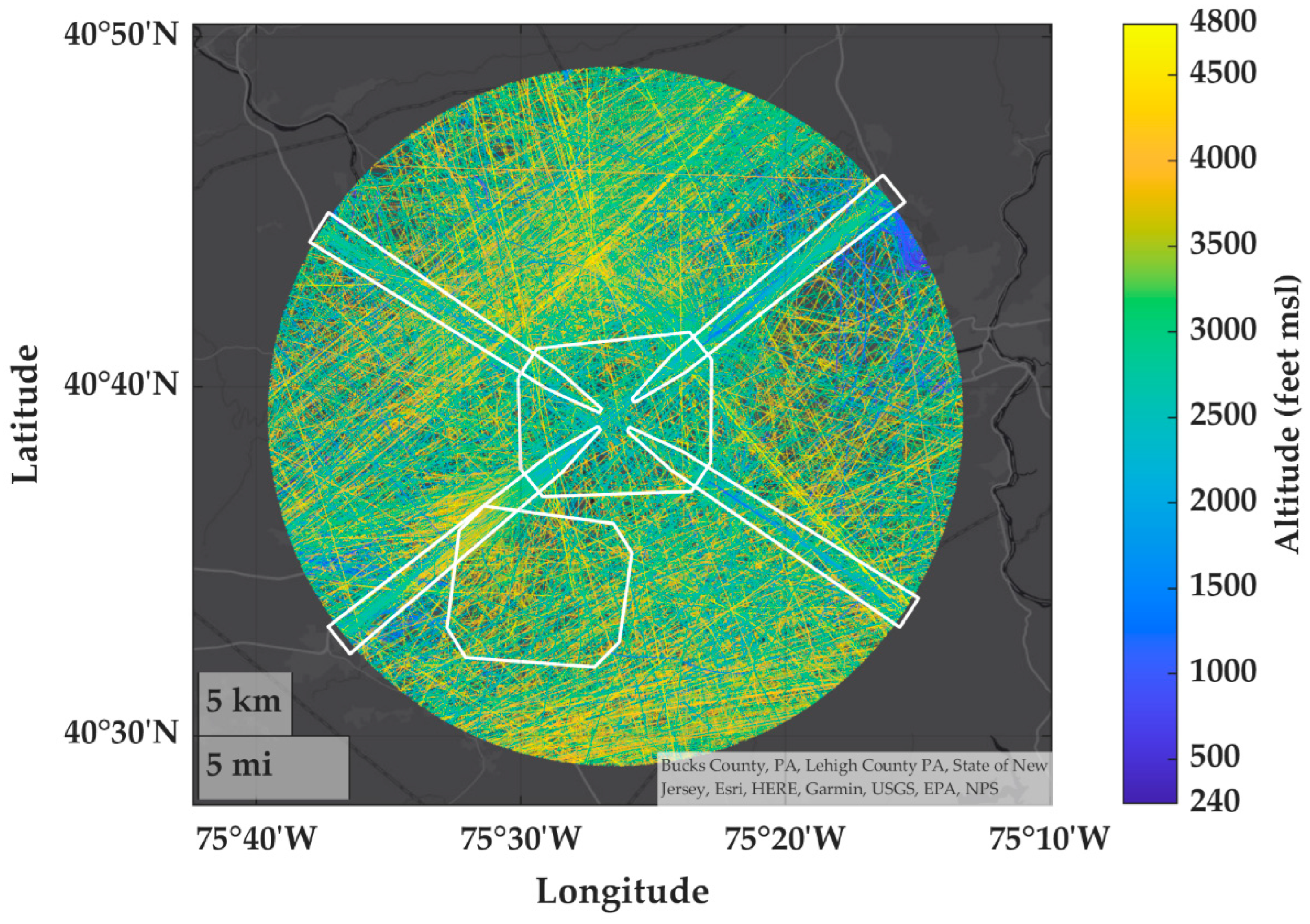
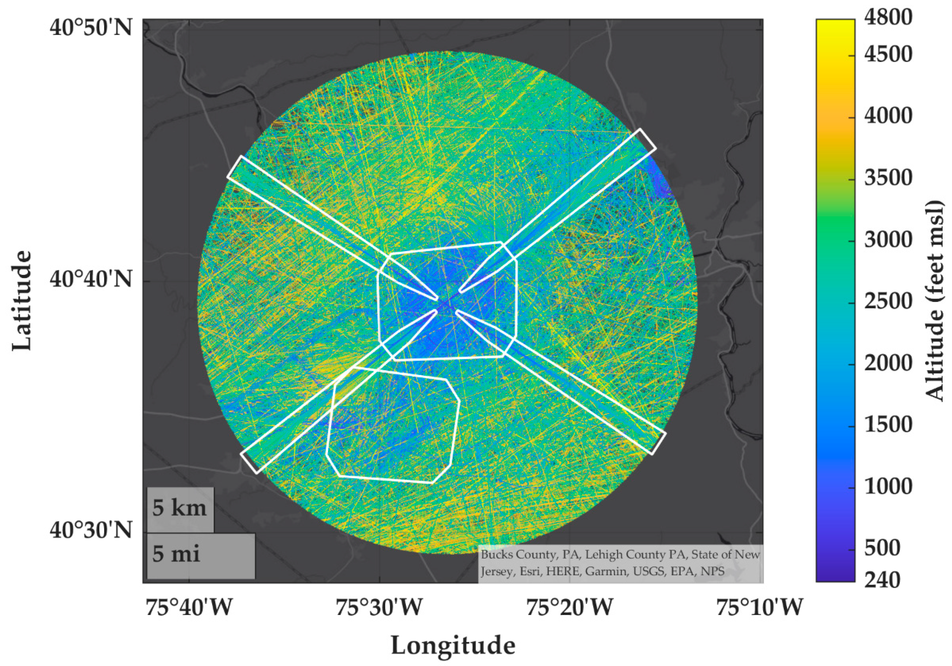
3.1. Initial Spatial Filtering

Initial spatial filtering was primarily executed to reduce the computational complexity and requirements subsequent processing steps. All track segments at least 30 s in duration (assuming one second updates), within a 10 NM radius of an airport of interest, and up to 4000 ft altitude relative to the airport surface were identified as within the vicinity of an airport. The FAA airport open dataset (https://ais-faa.opendata.arcgis.com/datasets/e747ab91a11045e8b3f8a3efd093d3b5_0, accessed on 5 November 2020) was used to define the latitude and longitude coordinates of the airports. Additionally, observations with transponders squawking specific special use transponder codes, such as those reserved for law enforcement aircraft, were also filtered out. Refer to Appendix C for a complete list of these codes. Tracks that did meet all these conditions were filtered out and not considered in the subsequent processing. Parallelized across 1008 xeon-e5 processes on the LLSC TX-Green with a block task distribution, 782 s was required to identify 19,293,916 OpenSky ADS-B tracks and 10,045 s for 36,701,193 terminal radar Mode C tracks.
To assess the potential local geospatial biases of the different datasets and visualize the surveillance coverage, we calculated the joint distributions of the relative distance and altitude between the airport and all the nearby data. The joint distributions are visualized as contours. While the initial filtering includes altitudes up to 4000 feet relative to the airport, the contours in Figure 1, Figure 2, Figure 3, Figure 4, Figure 5 and Figure 6 are illustrated with relative altitude up to 2500 feet for readability and to promote discussion about the lower altitudes, which are of greater interest. Across the figures, discussion focuses on airspace near Renton Municipal (RNT), Seattle-Tacoma International (SEA), Nantucket (ACK), Martha’s Vineyards (MVY), Laurence G. Hanscom Field (BED), and Boston-Logan (BOS).
Figure 1 illustrates distributions for RNT, a single-runway Class D airport approximately 4 nautical miles northeast of SEA. It supports colloquial statements such as “5% of the identified traffic based on the OpenSky Network near RNT was within 2 nautical miles and 1000 feet or less of the airport,” or “50% of the identified traffic based on the terminal area radar dataset was at least 6 nautical miles and 500 feet above RNT.” RNT exemplifies the effect of nearby airports on identified tracks. Because the OpenSky Network is a distributed network of sensors, there was potentially less of an observation bias towards one specific location. This bias was exemplified by the gradual gradient approximately 4 nautical miles from the OpenSky Network-based tracks and the steep gradient from the terminal area radars dataset. The terminal radar located at SEA was expectantly observing nearby very low altitude.
However, not all low-altitude traffic can be attributed to nearby airports. Of the more than 21 million points from the OpenSky Network dataset near RNT, 921,958 or approximately 4%, were associated with rotorcraft. Similarly, approximately 4% and 6% of OpenSky Network-based data were rotorcraft for Fort Lauderdale-Hollywood (FLL) and Addison (ADS), yet 12% and 15% were rotorcraft for BED and Sacramento (SMF). The tendency to observe rotorcraft operating at lower altitudes has also been observed when training the uncorrelated encounter models [7].
Next, we illustrate some the advantages and disadvantages of crowdsourced data by analyzing the Class D airports for ACK and MVY, islands off the southern coast of Massachusetts. The islands are more than 50 nautical miles from the nearest terminal area radar and approximately 26 nautical miles apart from each other.
Due to the distance away from the terminal radars, it was expected that neither airport would have any processed tracks from that dataset. Foremost, particularly with MVY, the OpenSky Network provided hundreds of flight hours for ADS-B equipped aircraft for a location where the other dataset had no coverage. However, these crowdsourced sensors often have limited range, which is exemplified by comparing the distance contours for ACK and MVY. These contours suggested that a sensor was located on Martha’s Vineyard, as MVY had relatively good low-altitude coverage but that all observations near ACK were also from this MVY-based sensor. See Appendix B for other examples of how surveillance coverage for a location differs between the datasets.
All of the discussed biases can be observed when comparing BED to BOS. BOS is located approximately one nautical mile from the densely populated downtown of Boston while BED is located in the less populated suburbs approximately 13 nautical miles away from BOS. This region is unique in that the terminal area radar, MOD, is located at BED, a Class D airport, and not BOS, the nearest Class B airport. The proceeding discussion suggests that BOS should benefit from a greater nearby population density for the OpenSky Network-based data and that BED should have a greater percentage of tracks below 500 feet for the terminal radar data due to the location of the radar. This hypothesis was supported by percent differences between BOS and BED, with BOS having 119.5% more observations for the Open Sky Network-based data and 72.3% more using terminal radar dataset. The percent difference indicates that a greater percentage of data was gained from switching the target airport of BED in the suburbs to BOS in the city. Additionally, note that for distances greater than 2.5 nautical miles with the terminal area radars, the 5% contour relative to BED is below 500 feet in Figure 5 but above 500 feet in Figure 6 relative to BOS. This indicates a greater percentage of low-altitude traffic below 500 feet observed by the terminal area radars were observed closer to the radar’s location at BED than away from the radar at BOS.
Figure 1, Figure 2, Figure 3, Figure 4, Figure 5 and Figure 6 all indicate that aircraft are rarely observed within 2 nautical miles and no more than 500 feet above airports. While the contours are dependent upon the surveillance performance, the general shape and conclusions drawn from the different airports are similar. The surveillance performance differs for each of the airports Figure 1, Figure 2 and Figure 3 also indicated that aircraft operate largely above 500 feet AGL. Assuming the contours are representative, the associated aircraft behavior aligns with many FAA regulations, such as 14 CFR § 91.119—Minimum safe altitudes or 14 CFR § 91.129—Operations in Class D airspace. Namely, aircraft rarely should operate low and close to airports and that the majority of the time aircraft are not operating in the terminal environment.

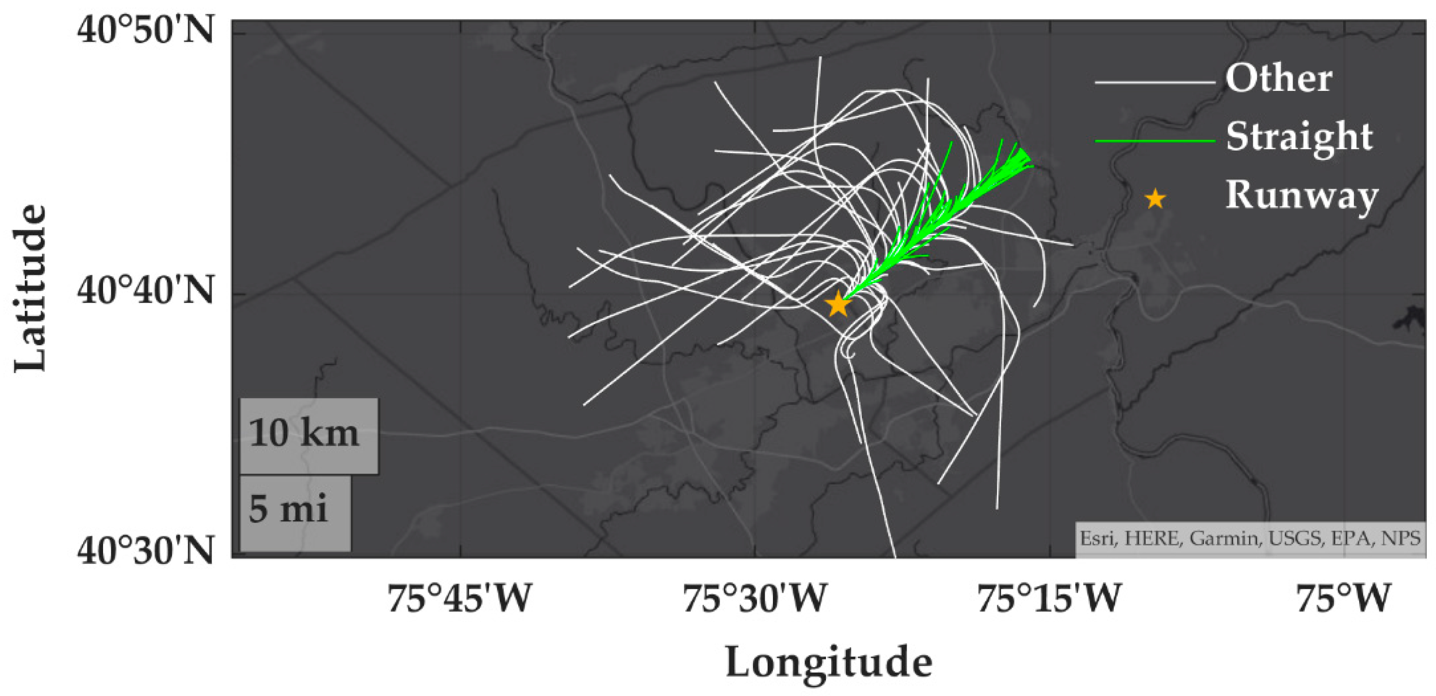
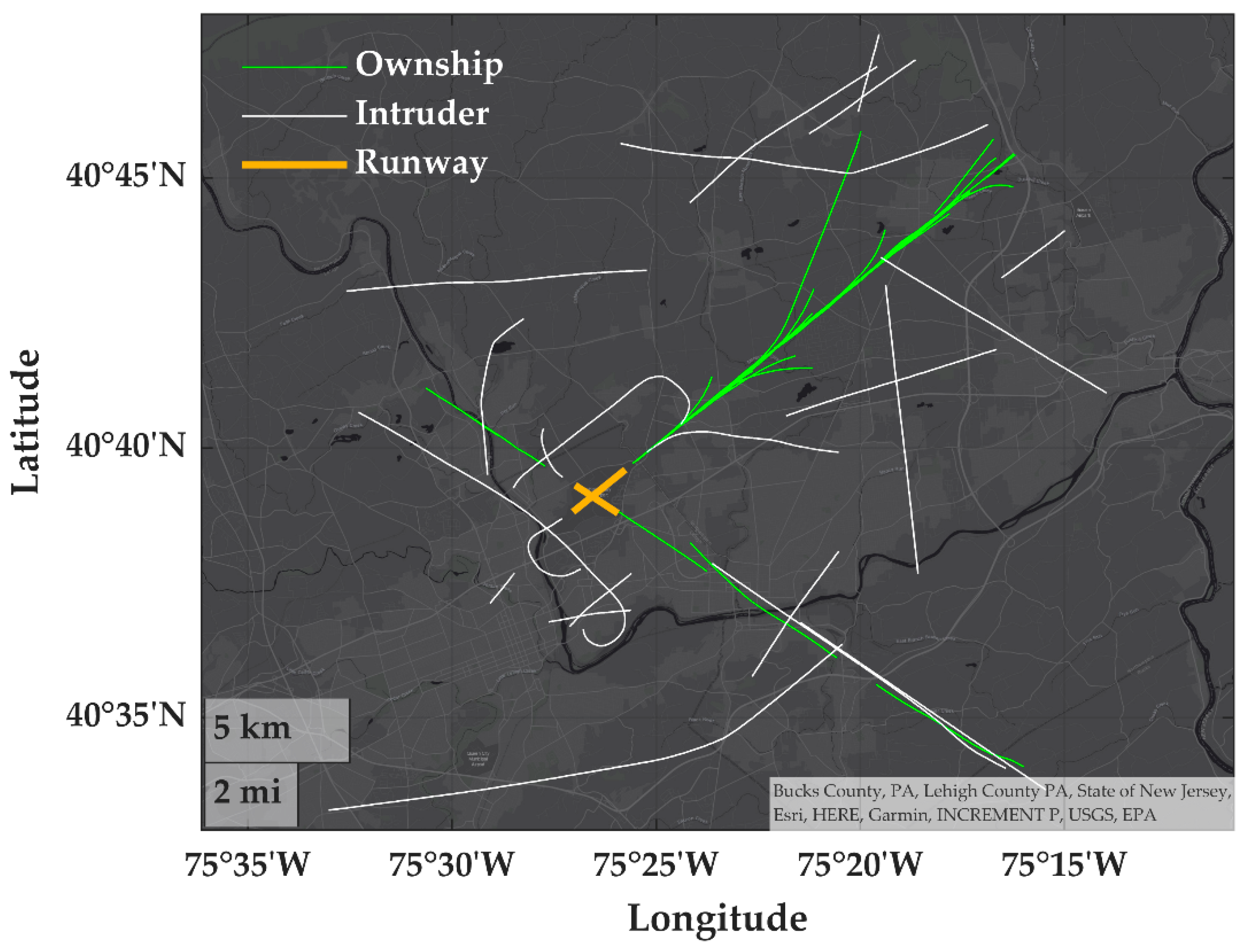
3.2. Track Intent and Runway Identification

After the initial filtering, we identified the intent for the tracks and which runway a track was interacting with when taking off or landing. Tracks are considered independently. For this processing step, there were six different intents identified. A transiting intent was indicative of a track not interacting with any runways and assumed to be transiting through the airspace. General aviation cross country flights or en route aircraft are example behaviors we sought to identify as transiting. There were two landing intents, straight and other, where straight corresponds to a straight-in landing and other is any other type of landing. Similarly, there were two takeoff intents, one for straight-out and another for all other types.

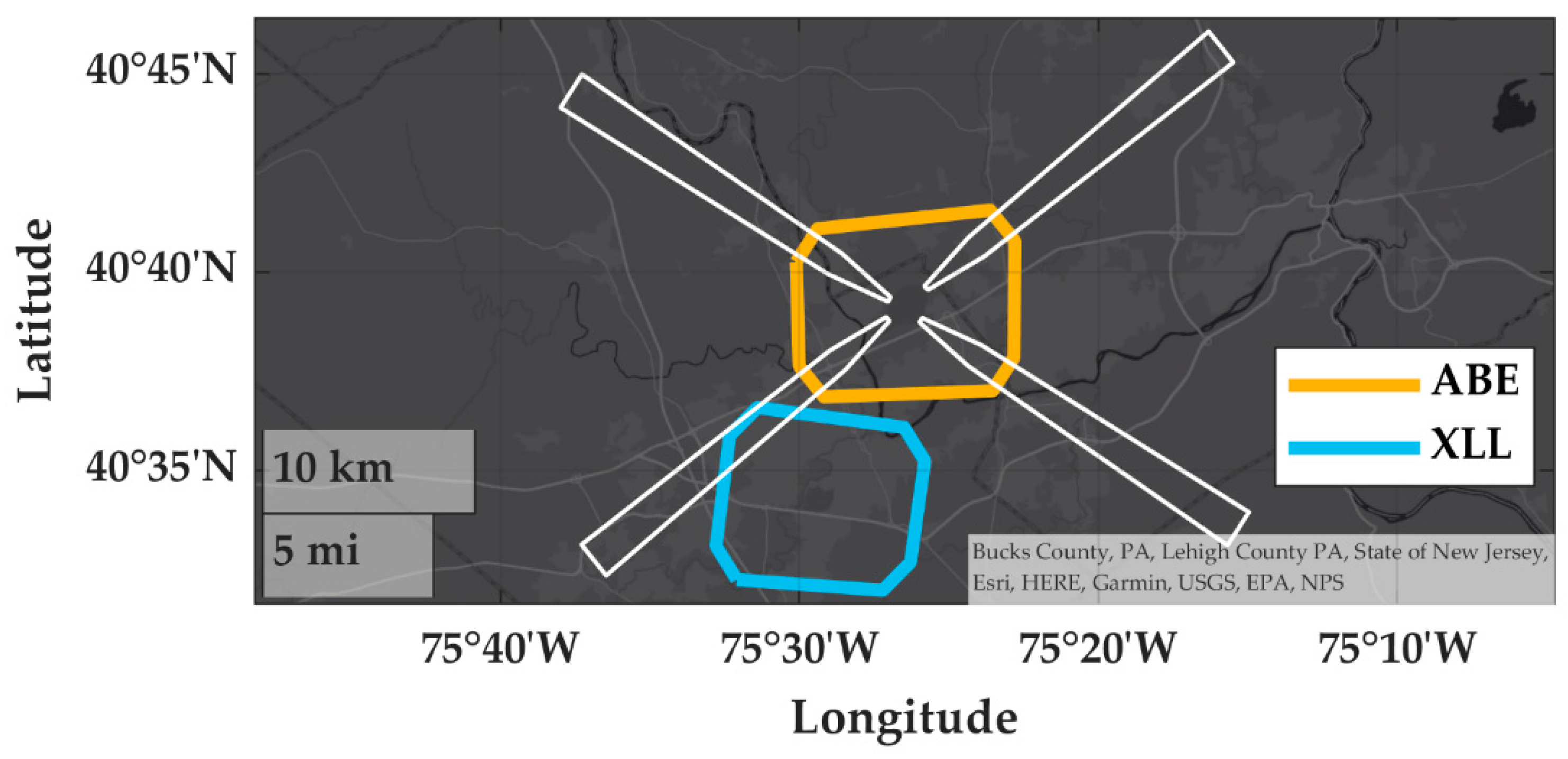
3.2.1. Clustering Using Airport Boundaries

First, we identified if a track was operating near the airport of interest or near any airports within 10 nautical miles of the airport of interest. For each airport, an airport bounding polygon was created based on assumed airport design and traffic pattern. Assumptions based on airport design and runway approach and departure standards were based on the FAA Advisory Circular (AC) 150/5300-13A, Airport Design, which could differ than the approach surfaces defined in 14 CFR § 77. For each runway, an approach and departure corridor was generated as trapezoids (isosceles trapezium) (Trapezoid shape based on dimensions B, C, D from Figure 3-2 and Table 3-2 from AC 150/5300-13A), extending 2.5 nautical miles out from the runway, and 800 and 3800 feet along the narrowest and widest parallel sides. The traffic pattern was estimated by a circle centered on the airport with a radius of 1.2 nautical miles, which is greater than the two miles, prescribed by the FAA airplane flying handbook [25], that aircraft should be to remain well clear from the pattern. To generate the airport boundary, a boundary was created around all the estimated approach surfaces and traffic pattern.
Figure 7 illustrates the boundaries for Newark Liberty (EWR), Downtown Manhattan/Wall Street (JRB), and Linden (LDJ) and shows that airport boundaries can overlap. Since the model assumes intruder aircraft are not taking off or landing from nearby airports, the proximity and overlap of airport boundaries was important. If a track flew through the airport boundary for any nearby airport, at any altitude, it could not be classified as taking off or landing from the airport of interest. Although this criterion was stringent, it was intended to minimize the risk of including undesired tracks landing and taking off from other airports when training the model.
Additionally, note that JRB is the Downtown Manhattan heliport without a fixed runway. Without runway information, no trapezoids were calculated and the airport boundary was just the traffic circle. LDJ has a single runway, so an airport boundary for LDJ based only on the trapezoids would be narrow and just as wide as the trapezoid which would insufficiently cover the traffic pattern. However, for larger airports, like EWR, the traffic circle may barely extend past the runways.

3.2.2. Clustering Using Runway Corridors

Next, if a track was within the airport boundary for only the airport of interest, we determined if the track was also within the runway two-dimensional approach and departure corridor. These corridors were similar to the airport boundary trapezoids but also extended 8 nautical miles from each runway (Shape based on dimensions B, C, D, E from Figure 3-2 and Table 3-2 from AC 150/5300-13A). A track must be in a runway’s corridor for at least 30 s. Each runway corridor was assessed independently and a track could be assigned multiple runways.
Figure 8 illustrate these corridors for Lehigh Valley International (ABE). The Allentown Queen City Municipal (XLL) airport boundary intersects with one of the ABE runway corridors. Given the requirement that a track can only intersect the airport boundary for the airport of interest, the majority of the tracks in the overlapping could not considered as taking off or landing from ABE.

3.2.3. Vertical Rate, Altitude, and Relative Heading

If a track segment satisfied the spatial and temporal requirements based on the runway corridor, it was furthered assessed based on vertical rate, altitude, and the relative distance from the runway. If these additional criteria were met, the track was classified as either taking off or landing. The vertical rate of the track when it was in the corridor was assessed to help determine if a track was taking off or landing. The vertical rate had magnitude and duration components. When in a corridor, the magnitude of the vertical rate had to be at least 300 feet per minute for a specific duration. This threshold duration could either be the time to vertically transit from the minimum and maximum track altitudes or 30% of the entire duration the track is in a corridor. These criteria also were iterated upon between version 3.0 and 2.0 of the models. It was initially 50% and 500 feet per minute but the initial criteria excluded tracks with many points in the corridors or with slower vertical rates near a runway. If the vertical rate was negative and the track decreased altitude, it was classified as landing; and vice versa for takeoffs.
To be classified as taking off or landing, when in a corridor, the track must fly within 2.5 nautical miles and 750 feet from the end of the runway of interest. This lateral and vertical criterion corresponds to the aviation heuristic 1 in 60 rule and an assumed 3 degree glide slope. This criterion was notably iterated on during model development. For version 2.0 of the model, the criterion was not based on an assumed 3 degree glide slope and was instead, 1 nautical mile and 475 feet.
Finally, to determine if the takeoff was straight-out or the landing was straight-in, we calculated the magnitude heading relative to the runway for all track points in the corridor. If the 95th percentile of all relative headings was 30 degrees or less, the track was classified with an intent of either straight landing or take off. Otherwise it was classified as a non-straight landing or takeoff. For straight takeoff and landings, any points immediately before or after the track enters or exits the corridor that satisfied a 40 degree relative heading threshold were also assigned a straight landing or take off intent.
For the other intents, a change in altitude criteria was used to classify points outside of a corridor. For takeoffs, after exiting the corridor, points until the maximum altitude was achieved were as labeled as with the takeoff intent. Conversely points descending from the maximum altitude prior to entering the corridor were labeled with a landing intent. For example, Figure 9 illustrates classified tracks for an ABE runway.

3.2.4. Transiting Aircraft

If the minimum altitude for all points within a corridor was greater than 1500 feet relative to the runway and the maximum altitude was less than 5000 feet, then the track would be labeled with an intent of transit. If a track intersected any airport boundary but none of the corridors, the same altitude criteria was applied to determine if the track was transiting over the airport. For example, any tracks that intersected solely the XLL boundary would need a minimum altitude of 1500 feet to be classified as transiting. This criterion was successful in filtering out low-altitude traffic operating from nearby airports, while not filtering en route traffic flying above the airport. Figure 10 illustrate transiting aircraft for ABE and Figure 11 illustrates the notional condition if the altitude criteria were changed from 1500 to 0 feet relative to ABE. Note the lack of low-altitude tracks colored blue within the centered ABE boundary in Figure 10 but the presence of low-altitude tracks in Figure 11. This difference illustrates tracks established in the traffic pattern around ABE that satisfied the airport boundary but failed to satisfied the runway corridors criteria. Also evident was the low-altitude traffic operating near XLL that was southwest from ABE and filtered out in Figure 10.

3.3. Encounter Identification

The previous step only identified the intent (e.g., landing, taking off, transiting) of independent tracks, the next step was to identify encounter between aircraft where the horizontal and vertical separation was simultaneously was 4 nautical miles laterally or less and 2000 feet vertically or less. First, for encounters where one aircraft had an intent of a straight-in landing or straight-out takeoff. we determined if there was at least one second overlap in UTC time, with potentially hundreds of thousands of encounters satisfying this temporal criterion. We then filtered to encounters with at least thirty seconds of overlap in time while satisfying the loss of separation requirement.

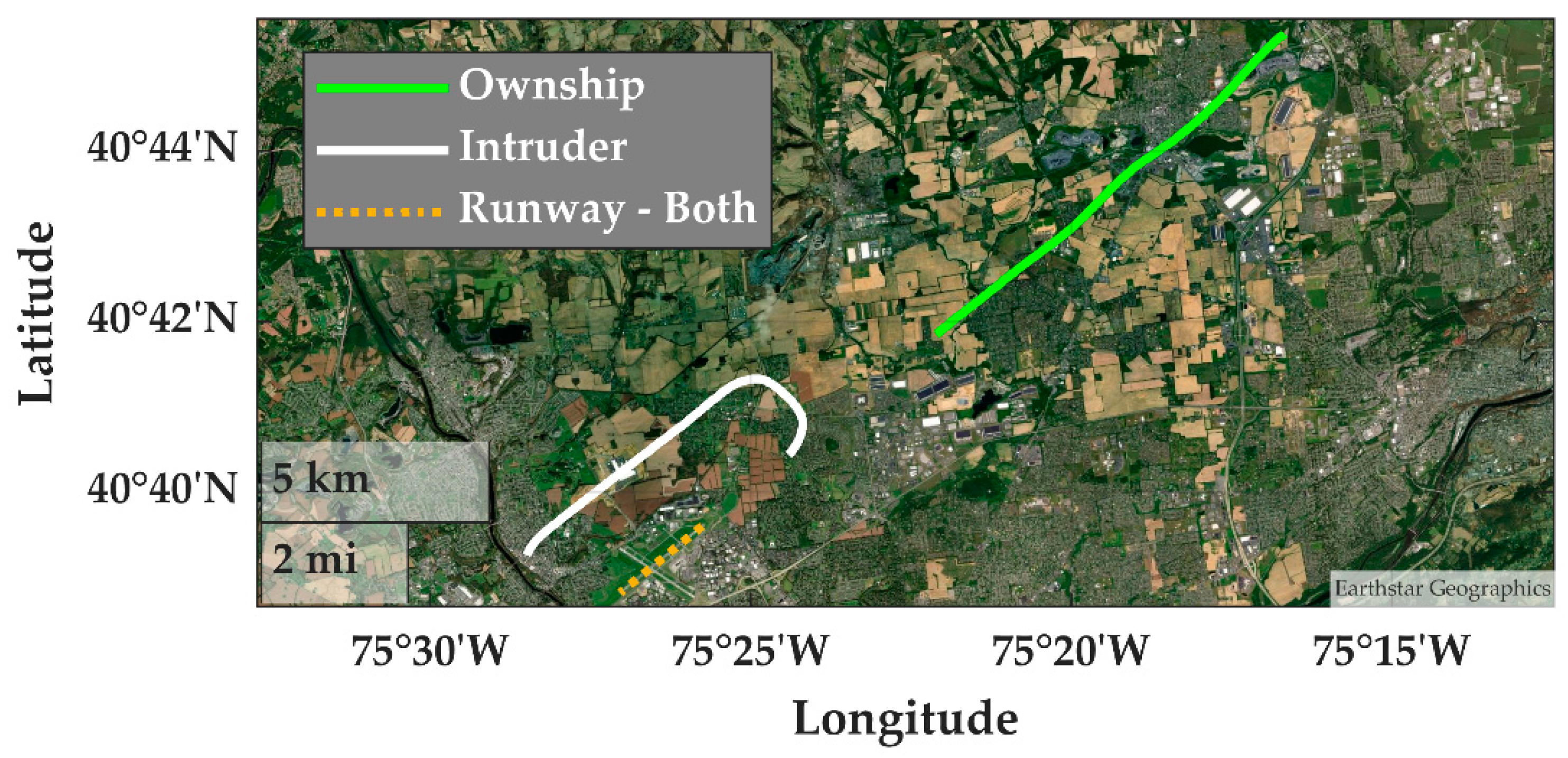
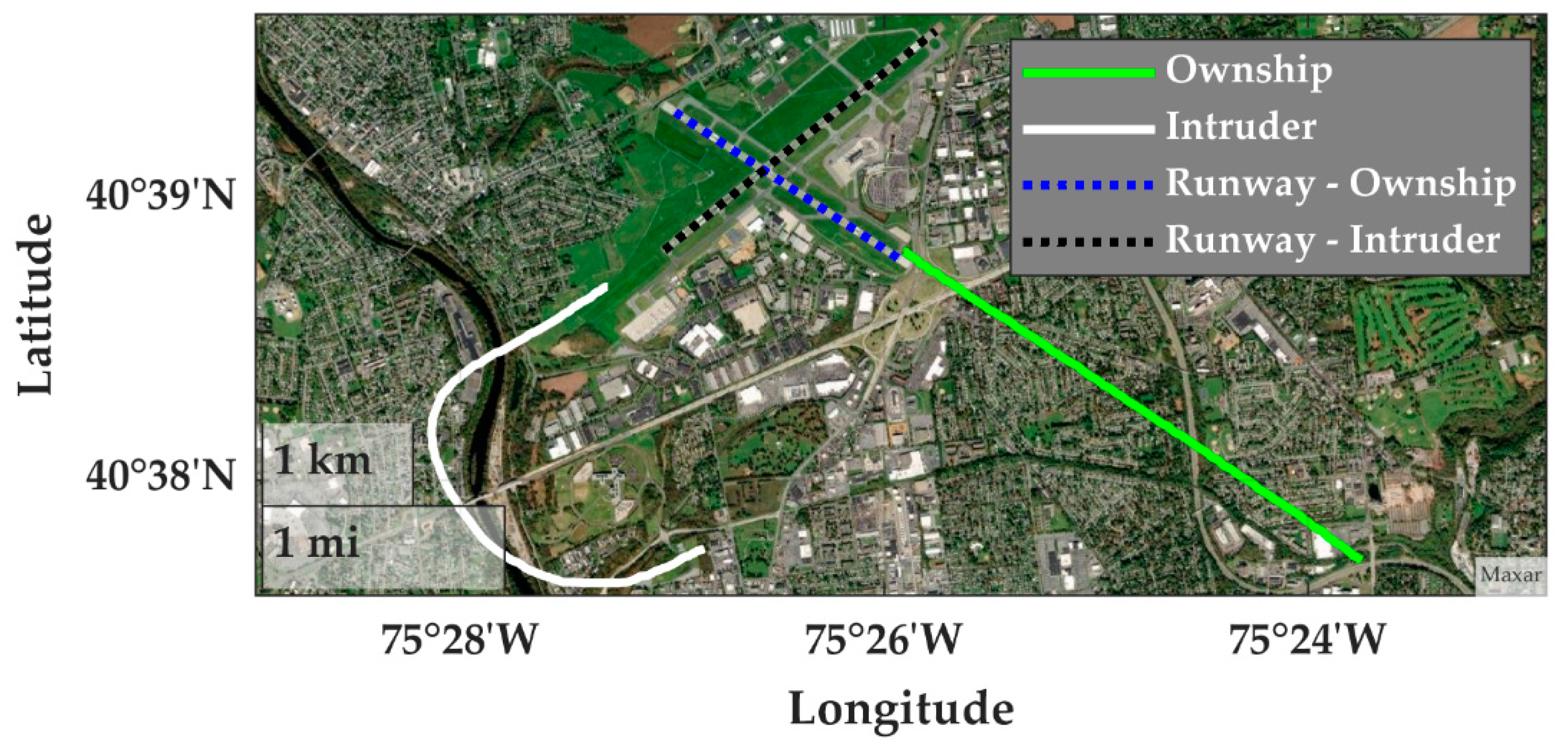
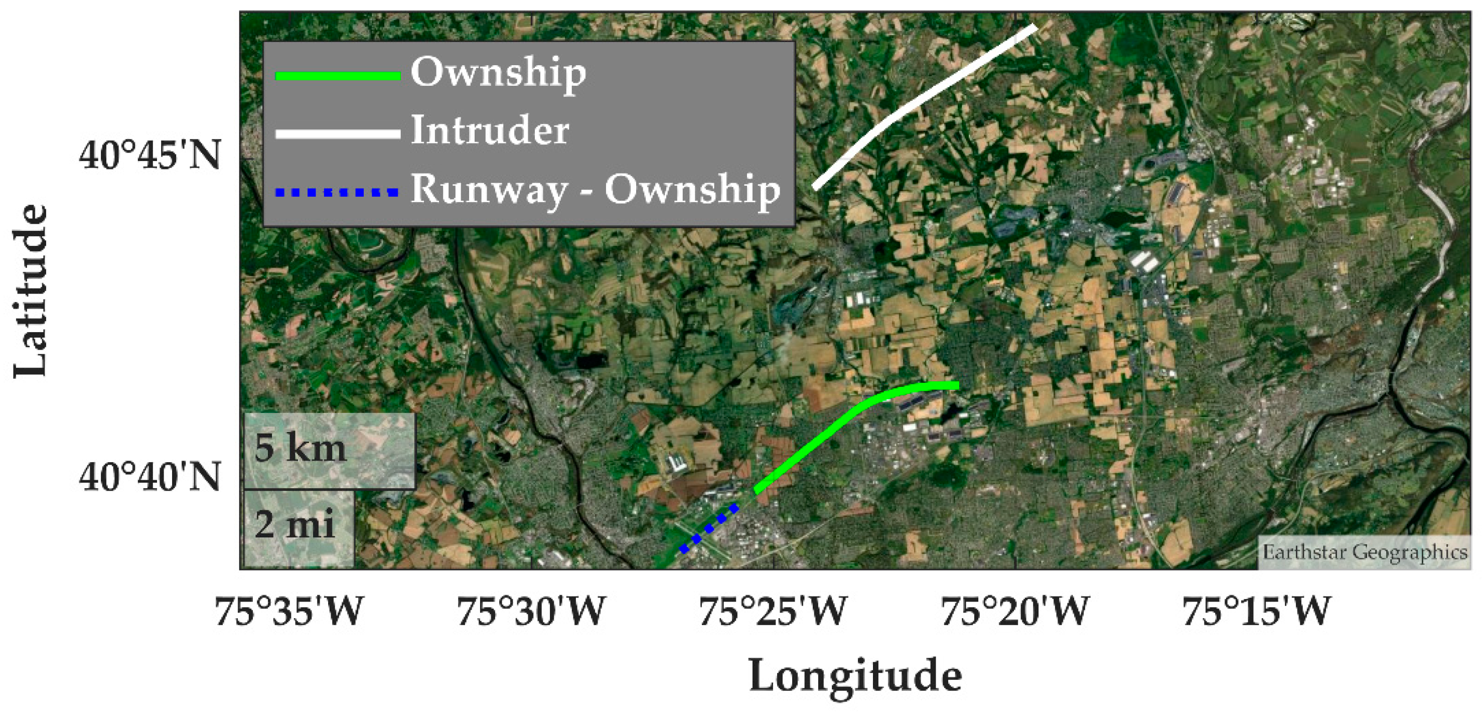
3.3.1. Example Training Encounters

Figure 12, Figure 13 and Figure 14 illustrate example encounters identified at ABE. Figure 12 and Figure 13 illustrates an encounter where ownship is landing and the intruder is either also landing or taking off. These figures highlight the heading constraints on the ownship. While both aircraft are landing, the final approach and landing for the intruder can be highly variable across encounters, whereas ownship must always have a minor relative heading difference from the runway. Figure 14 demonstrates that ownship may exhibit some minor turning behavior due to the relative heading threshold of 30 degrees or less and that aircraft, particularly intruders, can be oriented many nautical miles away from the runway.

3.3.2. Encounter Quantities

Table 2 summarizes how the data were filtered from the initial spatial filtering to the final set of identified encounters for three representative airports.
While we had significantly less data for ABE than LBJ, ABE had more potential encounters that satisfied the intent criteria for potential encounters and had more encounters identified. This was attributed to the differences of the airspace and design of airports near ABE or LBJ. In particular, the immediate proximity of LBJ to the larger EWR (Figure 13) resulted in the majority of the tracks filtered out for consideration as ownship. Furthermore, the majority of traffic was likely operating from or to EWR, so the large quantity of data was more reflective of EWR than the smaller LBJ. Similarly, as discussed in Section 2.2, we observed significantly more traffic near ADS due the greater population density of the Dallas Fort Worth metroplex and increased traffic around the Class B airports of DFW and DAL. While ABE had less than one-tenth of the data as ADS, more potential ownship tracks were identified per observation points for ABE than ADS. Appendix D illustrates the identified encounters for ABE when using the aerodromes dataset.
Table 3 reports the number of encounters used to train the current encounter geometry model given airspace class and data source. While the OpenSky Network-based training dataset had a greater spatial and temporal scope, it was limited to only identifying encounters between aircraft that both had ADS-B equipped.

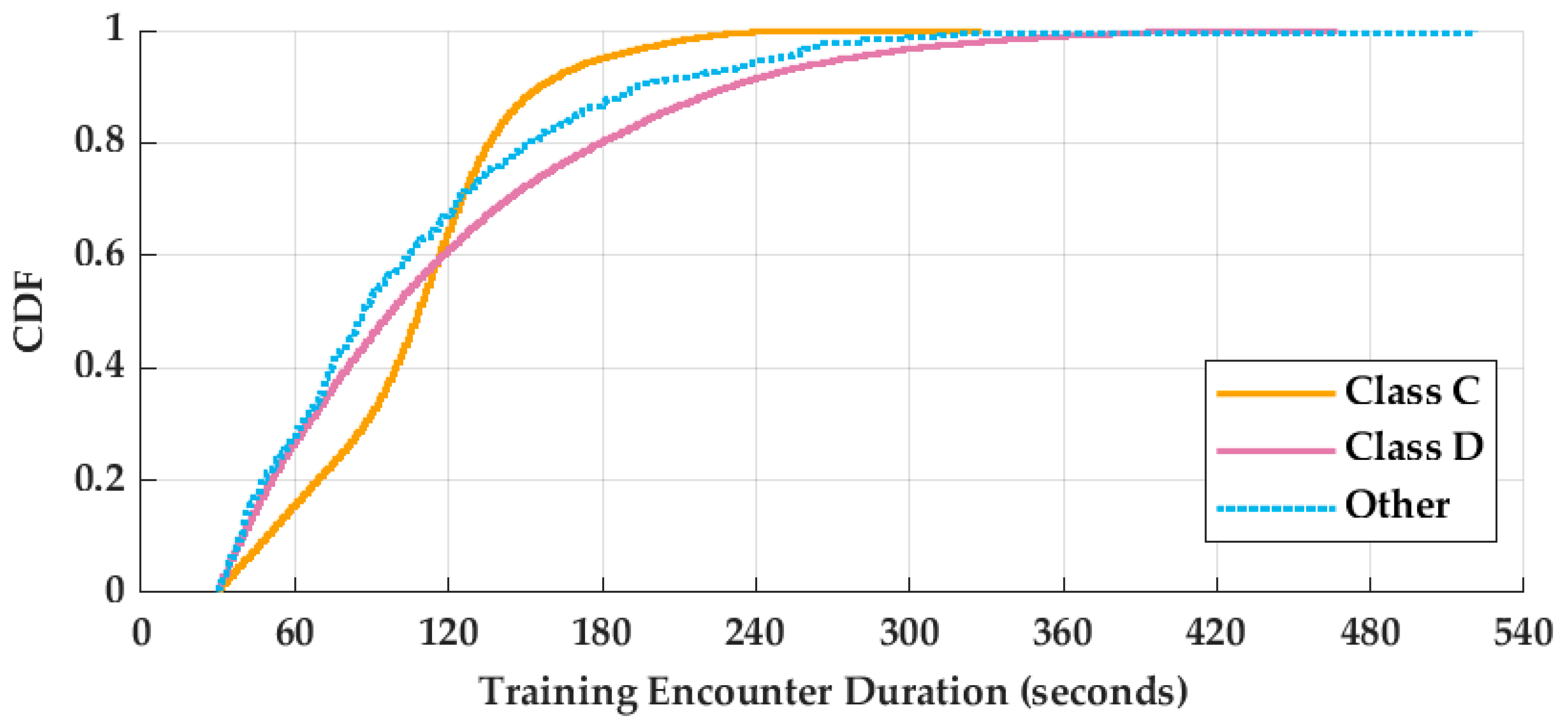
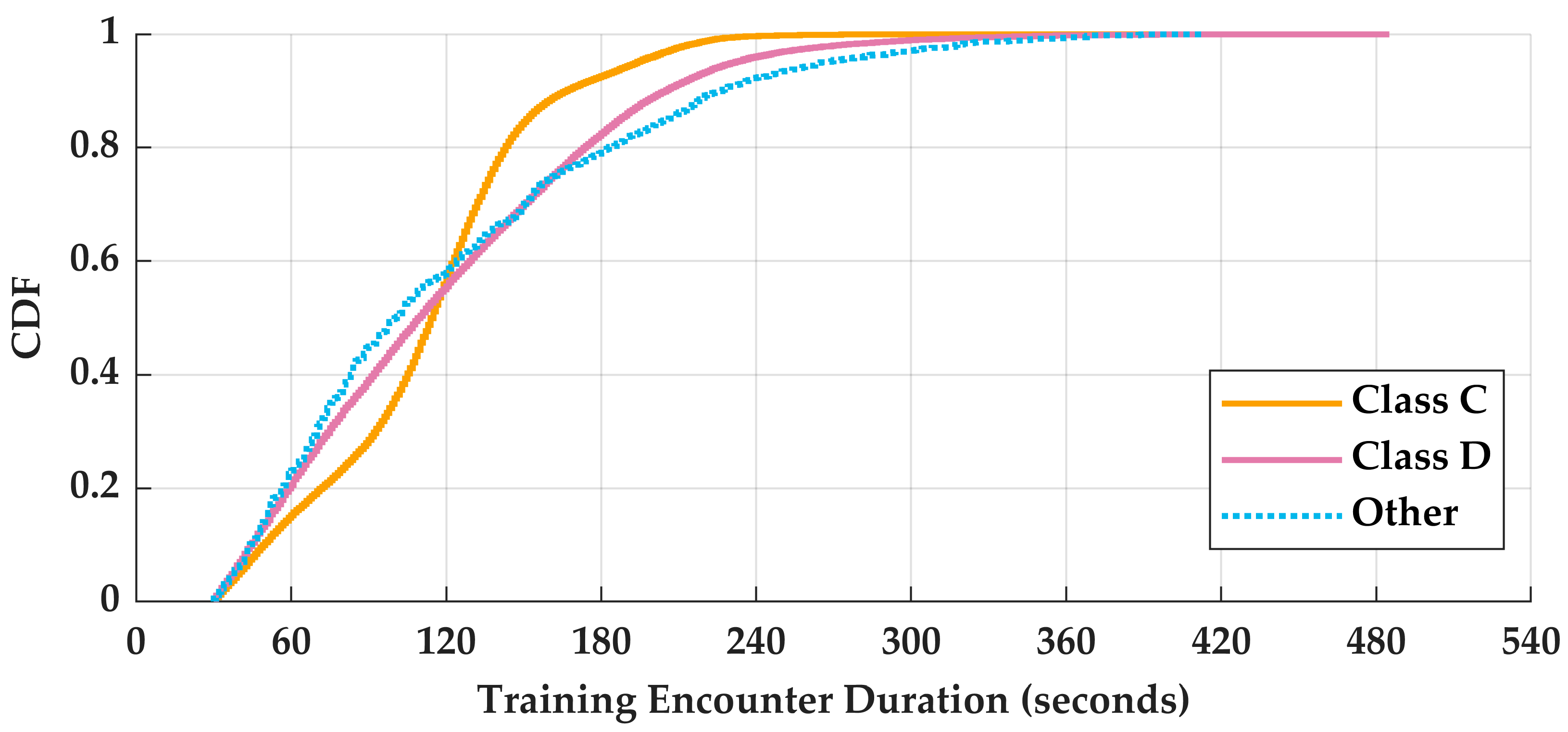
3.3.3. Encounter Duration

For all airspace classes when using the aerodromes dataset, the median duration of identified encounters for model training was at least 87 s and 10% or fewer encounters had a duration of 39 s or less, as illustrated by Figure 15. The median was at least 100 s when using the terminal area radars dataset. These two statistics indicate that the requirement for an encounter to be at least 30 s was not overly burdensome and not a significant factor when rejecting an encounter for model training. Figure 16 illustrates if the duration requirement increased to 60 s when using the aerodromes dataset, approximately one-third of the current Class D and other encounters would be rejected, while only 15% of Class C encounters would be rejected. Comparably, approximately one-quarter of the current Class D and Other encounters and a smaller percentage of Class C encounters would be rejected when using the terminal area radars dataset.
While the duration of training encounters had a minimal dependence on airspace class or dataset, the quantity of encounters identified for each airport of interest was biased towards a small percentage of airports. Table 4 reports the distribution of how many encounters were identified for an airport. For example, Table 4 reports that no encounters were identified for 29 Class C airports and that at least 100 encounters were identified at 24 Class C airports when using the OpenSky Network-based aerodromes dataset.
94% of the Class E or G (Other) airports when using the OpenSky Network-based aerodromes dataset and 89% of other airports with the terminal area radar dataset had no encounters identified. For the terminal area radars dataset, 48% of encounters in Other airspace were identified from 1% of the airports (n = 4) with any data after the initial spatial filtering.

4. Training the Dynamic Bayesian Network

This section describes the model structure, rejection sampling of the model, and example sampled encounters from the model.

4.1. Model Training and Structure

With encounters identified, the statistical models could now be trained. The terminal model consisted of an encounter geometry model and a trajectory propagation model. The first component, the encounter geometry model, describes the geometrical conditions of two encounter aircraft at their point of closest approach. The second component, the trajectory generation model, then describes the flight path for each aircraft leading to and continuing from their point of closest approach. Like the RADES-based correlated model, this was a generic model with no dependency on geography or locations.

Relative Local Coordinate System

Encounters are described in a coordinate system where all altitudes are relative to the mean runway elevation. Angular units are represented on a standard polar grid increasing in counterclockwise orientation. When training the model, the aircraft trajectories are rotated using a two-dimensional rotation matrix such that the runway the ownship is using lays directly on the y-axis, with the runway mean position located at (0,0). The runway is assumed to be a single point, rather than a vector or polygon. When training the model, positions and distances are relative to the mean runway position for the airport of interest. Since we trained a generalized model, this is a potential source of bias and error, as the mean runway position will vary for different airports.
Additionally, the runway is oriented above ownship on the y-axis: that is, ownship has a relative angular position (bearing) with a range of [180, 360] degrees. When projected onto a Cartesian coordinate system, the y-axis is oriented from 270 to 90 degrees, and x-axis from 180 to 0 degrees.
Figure 17 illustrates the bearing distribution for the ownship forward trajectory model, with similar distributions within the ownship backwards trajectory model. As bearing is a relative position, the distribution given a landing or takeoff intent are similar.
Bearing is the angular position, whereas heading is the correspondingly angular vector, that is the direction of flight. Figure 18 illustrates the heading distribution for the ownship forward trajectory model. Unlike the bearing distribution in Figure 17, the heading distribution is dependent upon whether ownship is taking off or landing. When landing, the average heading is 90 degrees, as the ownship is flying along the negative y-axis towards the mean runway position at (0,0); whereas when taking off, the ownship is flying away from the runway such that the mean heading is 270 degrees. The heading and bearing also reflect that ownship takeoffs and landing were constrained to be straight-out or straight-in; the distribution for the intruder models are different with the distribution over a wider range of values.
The differences with the intruder distributions is best illustrated by Figure 19 with the bearing and heading distributions of the intruder forward trajectory model given that the intruder is transiting through the airspace. Compared to the more constrained ownship distributions, the intruder distribution has a wider distribution over bearing and a significantly more encompassing distribution over the full 360 degrees range of headings. The intruder bearing distribution is reflective of the encounter separation criteria. Since ownship predominantly has a bearing in the range of [260, 280] degrees and encounters occur when aircraft are close to each other, it is not surprising that the intruder has a similar mean bearing. However, since transiting intruders are not flying to or from the mean runway position at (0,0), they operate more liberally throughout the airspace, as represented by the more diverse heading distribution.

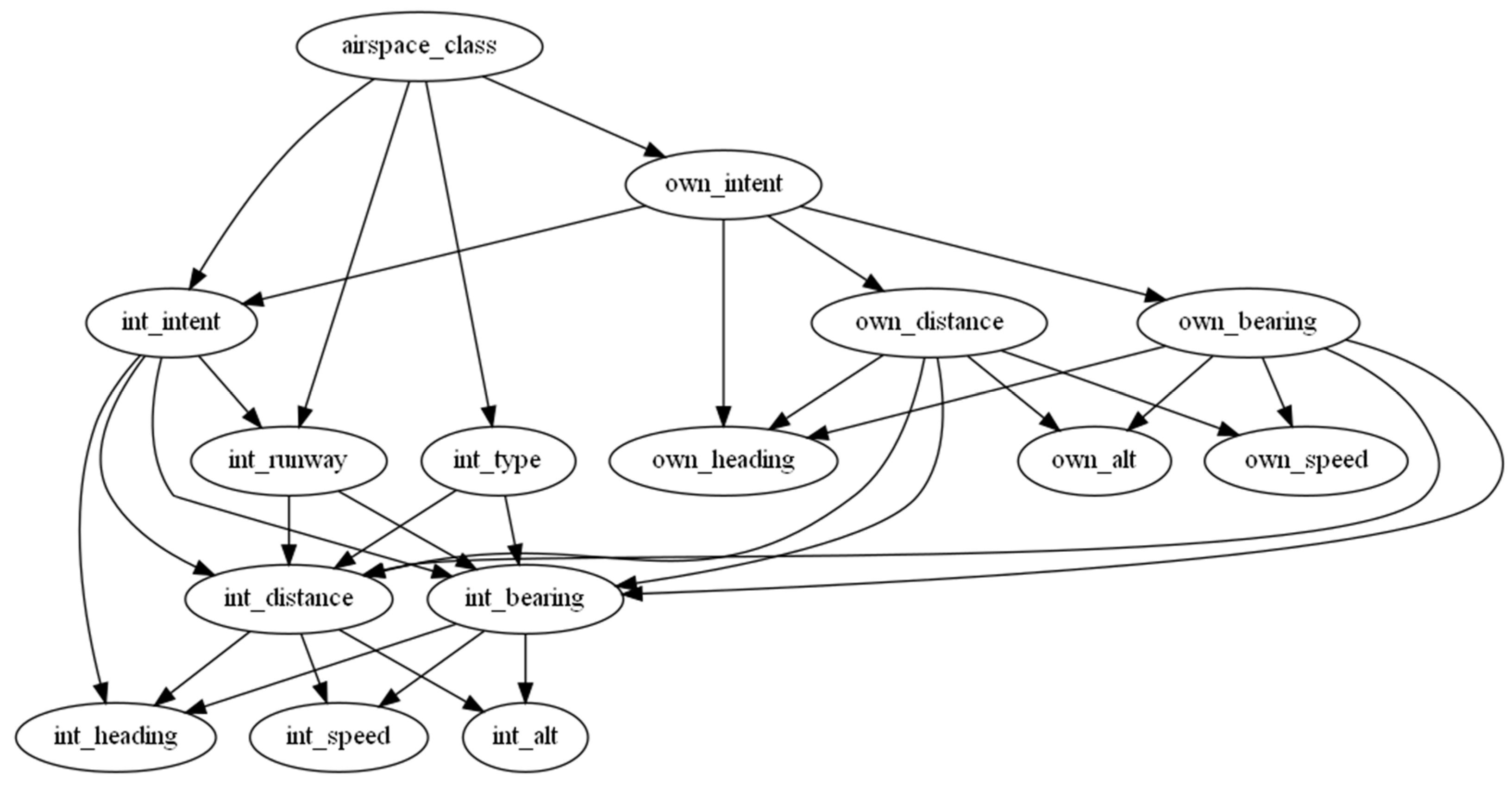
4.2. Encounter Geometry Model

The encounter geometry model describes the position, speed, and direction of two aircraft at their horizontal closest approach. Some variables were smoothed using a locally weight temporal smoother with a Gaussian kernel. It uses the following variables:
  • Airspace class: Airspace class of the airport.
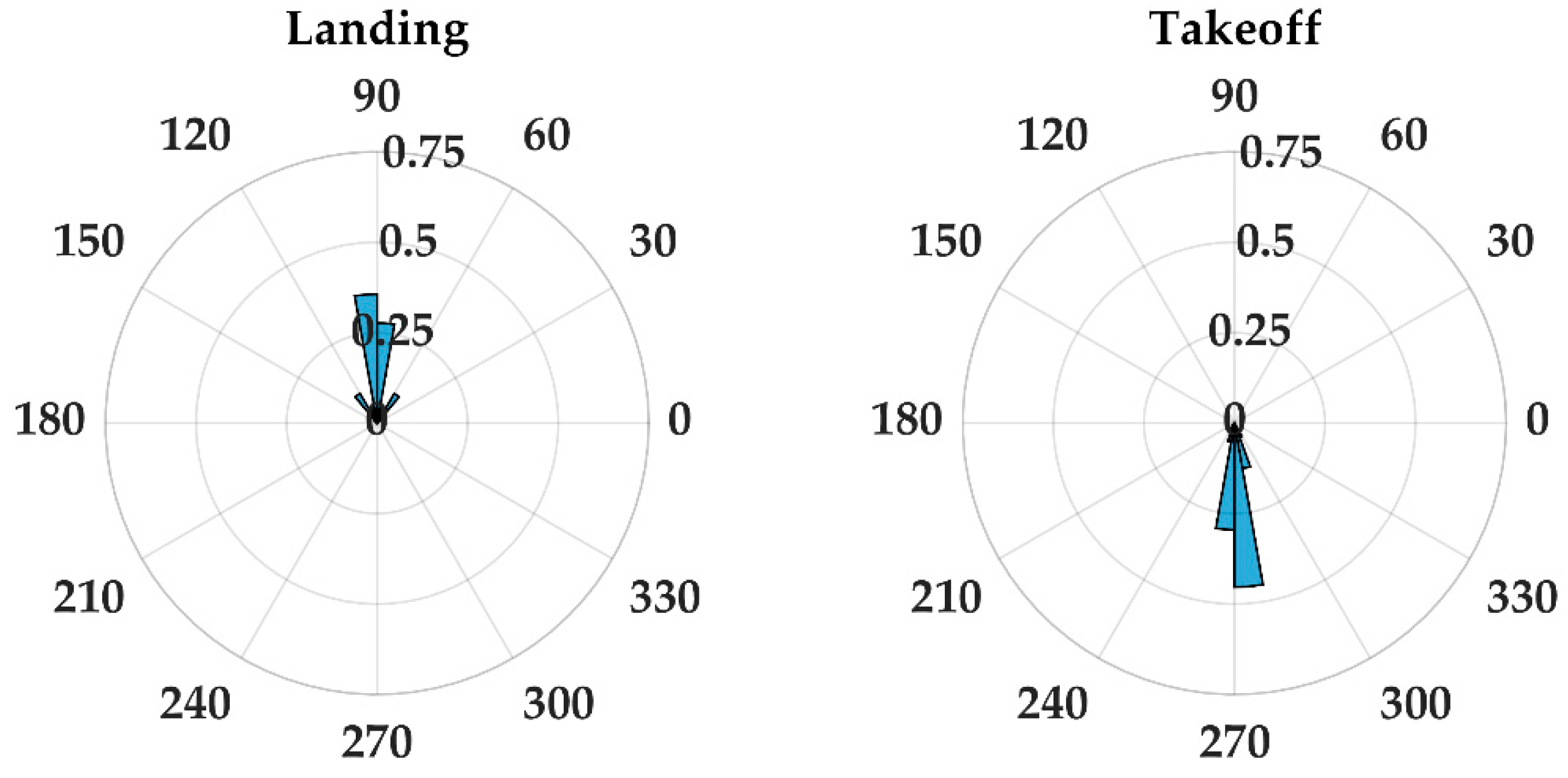
  • Ownship intent: The intent of the ownship of either a straight landing or take off.
  • Intruder intent: The intent of the intruder of either landing, taking off, or transiting. Unlike the ownship, the intruder’s intent is not assumed to be straight.
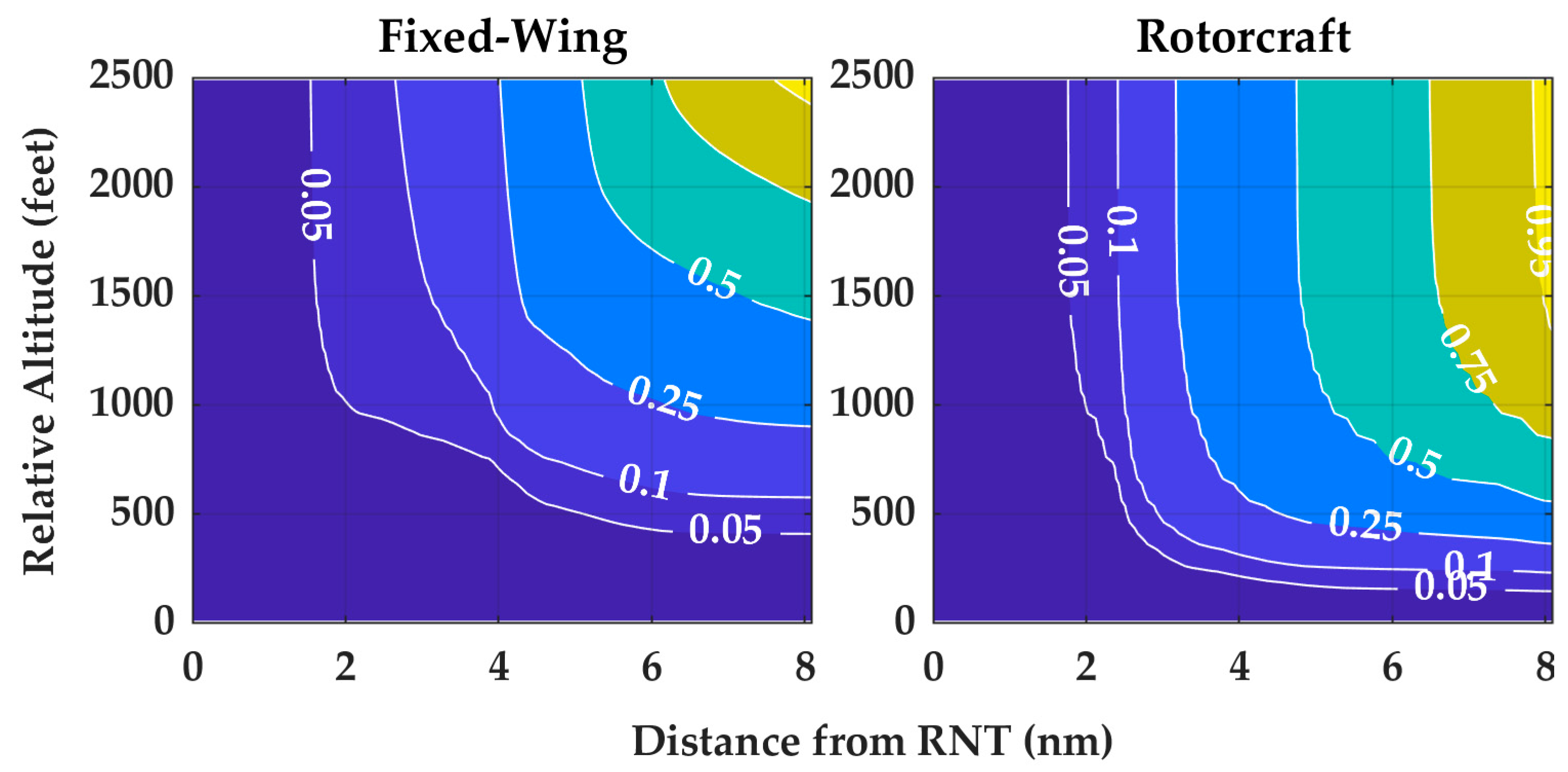
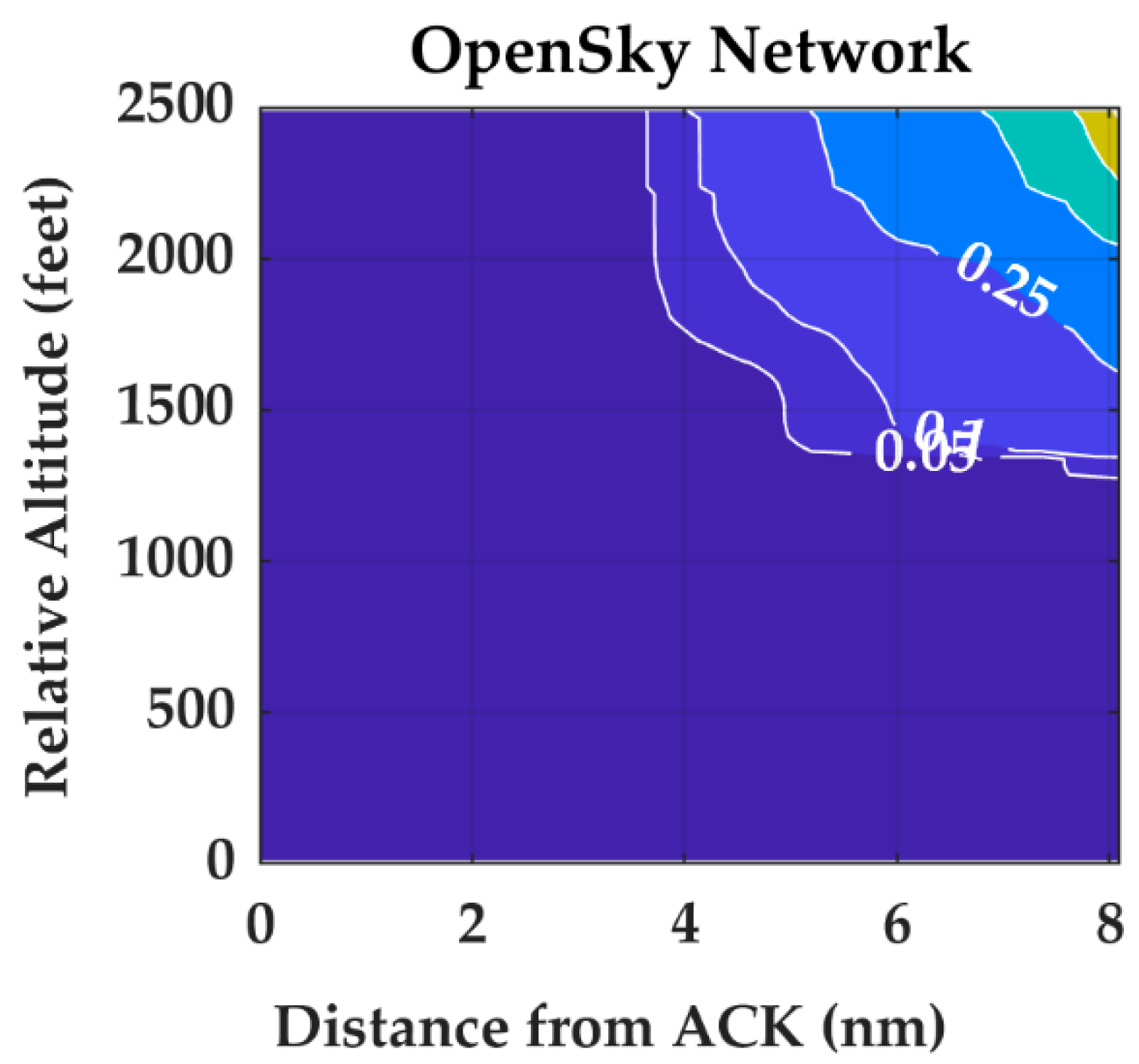
  • Intruder type: The type of aircraft of the intruder: can either be fixed-wing or rotorcraft. Note that while the OpenSky Network-based uncorrelated models are individually organized by aircraft type [7], aircraft type is an explicit model variable here.
  • Intruder runway: The runway the intruder was leveraging relative to the ownship. Designated as “same” if both aircraft were operating from the same runway; parallel” if the intruder was operating from a runway that did not intersect the ownship’s runway; as “crossing” if the intruder was operating from a runway that intersected the ownship’s runway; and “none” if the intruder intent was transiting.
  • Ownship distance from runway: The horizontal distance between the ownship position at CPA and the runway mean position.
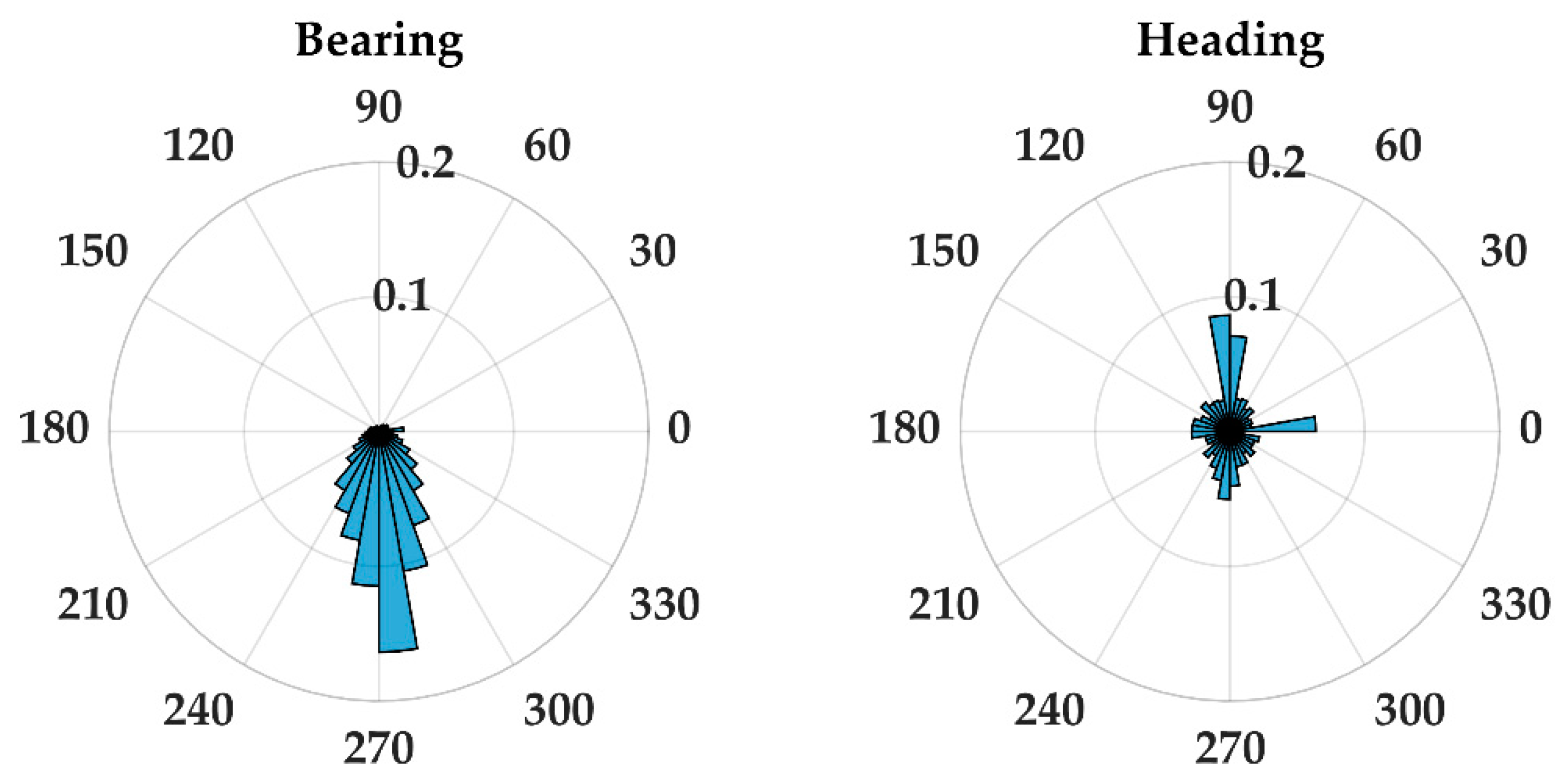
  • Ownship bearing from runway: The polar angle of the ownship’s position at CPA.
  • Ownship altitude: The altitude of the ownship relative to the runway elevation at CPA.
  • Ownship speed: The smoothed speed of the ownship at CPA as estimated by a finite difference of the trajectory position data.
  • Ownship heading: The direction of flight of the ownship at CPA.
  • Intruder distance from runway: The horizontal distance between the intruder position at CPA and the runway mean position.
  • Intruder bearing from runway: The polar angle of the intruder’s position at CPA.
  • Intruder altitude: The altitude of the intruder relative to the runway elevation at CPA.
  • Intruder speed: The smoothed speed of the intruder at CPA as estimated by a finite difference of the trajectory position data.
  • Intruder heading: The direction of flight of the intruder at CPA.
These variables were associated via a graphical model (Figure 20) that indicates dependency relationships. Those variables in turn are dependent on several other variables. In this graph, the variables are nodes and the dependencies are directed edges. The model has conditional probabilities, so the graph can be referred to as a Bayesian network.
Some variables, as identified in Table 5 below, are inherently discrete. Other variables, identified in Table 6 below, are inherently continuous. For representation in this model, the continuous values in the observed data must be discretized during training.

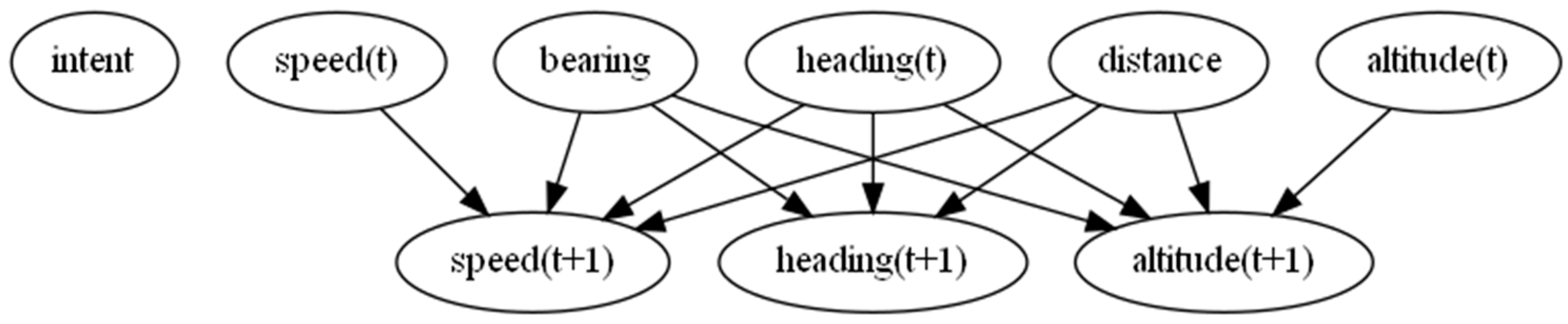
4.3. Trajectory Propagation Model

The trajectory generation models describe how the position of the two encountering aircraft evolves before and after their closest point of approach (CPA). While the encounter generation model considered the relatively geometry between aircraft, the trajectory propagation models assumed track independence, with ownship and intruder models trained separately. The training data for this model were the independent sets of ownship and intruder tracks from identified encounters.
The ownship and intruder trajectory propagation models have a similar model structure with a difference in the temporal variables. The forward propagation models transition from time (t) to (t + 1) after CPA has occurred, while the backwards propagation model is for time (t) to (t − 1) prior to CPA. Specifically, they use the following variables:
  • Intent: The aircraft’s intent, same as defined for the encounter geometry model;
  • Distance from runway: The horizontal distance between the aircraft position and the runway mean position over time;
  • Bearing angle from runway: The polar angle of the aircraft’s position;
  • Heading angle: The direction of flight of the aircraft;
  • Altitude: The altitude of the aircraft relative to the runway elevation over time;
  • Speed: The smoothed speed of the aircraft over time as estimated by a finite difference of the trajectory position.
Similar to the encounter geometry model, the trajectory model is also a Bayesian network but since the trajectory models also incorporate time dependencies, it is referred to as a Dynamic Bayesian network. This model structure was based on the Dynamic Bayesian network of the uncorrelated encounter models, which did not model distance or bearing with respect to some spatial point. Illustrated in Figure 21, the aircraft’s track at the next time step is dependent on its current track, its bearing from the runway, and its distance from the runway.
All variables in the trajectory generation model, defined in Table 7, are inherently continuous. Some cutpoints are different from those for the same variable in the encounter geometry model (e.g., altitude is more finely discretized here). For a given training dataset, different forward and backwards propagation models are trained for each intent of landing, taking off, and transiting. Forwards propagation models are trained on time-ordered trajectory data while backwards propagation models use reverse-time-ordered trajectory data for training. Future work may consolidate these models.

4.4. Model Sampling and Encounter Generation

Once the model has been trained with the observed trajectory data, it can be sampled to generate new encounters (“synthetic encounters”). Encounter generation is completed in three steps: sampling the geometry model, sampling the trajectory models, and rejecting or accepting the encounter based on general assumptions or aircraft performance.

4.4.1. Sampling the Encounter Geometry Model

First the encounter geometry is sampled to generate aircraft positions at CPA given distance and bearing relative to a runway’s mean position. The encounter geometry model is sampled with a uniform prior (i.e., absent any additional information, that all combinations of variables are equally likely). Figure 22 and Figure 23 illustrate 500 samples from the geometry model where ownship is taking off and the intruder is landing or transiting.
These figures illustrate two important elements of the model. First, the coordinate system is oriented such that ownship’s runway is parallel to the y-axis, with positive down the runway from the threshold. This results in ownship predominately operating to the “south” of the runway and the cone shape of ownship’s position is indicative of the 30 degree heading requirements for a straight landing or taking off. Second, the intruder position is dependent on its intent. Note in Figure 22 that a cluster of intruder positions are near (0,0). This cluster is not evident in Figure 23 and when transiting, the intruder at CPA is more dispersed. This was expected as transiting aircraft should not be operating predominantly along an approach or departure route. This is an outcome of the intent classification described in Section 2.3 and visually demonstrates how encounter geometry is dependent on aircraft intent.

4.4.2. Sampling the Trajectory Models to Propagate Tracks

Next, the ownship and intruder trajectories are successively sampled using the associated forwards and backwards trajectory generation models. Trajectories are propagated up to 120 one second timesteps before and after CPA, with initial positions provided by the geometry model sample. Propagation is achieved by successively sampling a trajectory model’s variables from the top of the graph to the bottom, applying the learned conditional probabilities in conjunction with Bayes Rule. The trajectory models are sampled using a non-transitioning prior: absent observed information, dynamic variables remain constant. It is important to use these priors because the large space of discrete-valued variable combinations make it likely that there are gaps in the conditional probability tables. Sampling only gives discrete values for each of the model variables. Continuous values for the continuous variables must subsequently be sampled. In all cases, the model assumes this sampling will be from a uniform distribution within the relevant bin.
Unlike previous encounter models, with which all transition events throughout an encounter can be sampled at once, the trajectory models can only be applied one time step at a time, with the new aircraft position being computed after each step. The new aircraft position is used to calculate the distance and bearing the track is away from the runway, with distance and bearing being model variables. This is required because distance from or bearing to the runway are not temporal variables in the Dynamic Bayesian network.
Additionally, unlike other MIT LL developed models, tracks do not need to fully overlap in time. It is possible for an encounter to start or end with only one aircraft in the vicinity of the runway. For example, an encounter could start at t = −120 s (prior to CPA) with the intruder initially positioned within 8 nautical miles of the runway. An ownship could be initialized at t = −30 s near the runway at a low altitude to simulate the ownship beginning to takeoff. In this example, CPA would occur at t = 0. At t = 30 s, the intruder could be more 8 nautical miles from the runway and no more track updates would be generated for it. From t = 31 and onward, only ownship would be simulated.

4.4.3. Rejection Sampling

Given an encounter of two aircraft tracks, we assess if its valid or should be rejected. If an encounter fails any of the described criteria, it is rejected and the encounter generation process is restarted with a new sample from the encounter geometry model. Criteria are organized into three categories: those based on training assumptions, assumptions unique to ownship, and dynamic constraints. The criteria based on training assumptions are designed such that the sampled synthetic encounters are subject to similar constraints and assumptions used to identify encounters for training:
  • Encounter CPA must occur within 5 s of the sampled CPA;
  • Tracks must overlap at least 30 s in time;
  • If taking off or landing, a track must have at least one track update within 2.5 nautical miles of the runway mean position;
  • For track updates within 2.5 nautical miles of the runway mean position, at least one point must have an altitude of 750 feet or less;
  • A track must have sufficient quantity of updates with a vertical rate magnitude of 300 feet per minute or greater. If landing, the rate must be negative and if taking off, the rate must be positive;
  • A track ends if it is within 0.25 nautical miles or more than 8 nautical miles away from the runway.
Similar to when classifying track intent, ownship must satisfy a relative heading criterion, so it is representative of a straight landing or takeoff. The ownship heading criteria is dependent upon intent:
  • If landing, at least 95% of heading updates need to be 90 ± 30 degrees;
  • If taking off, at least 95% of heading updates need to be 270 ± 30 degrees.
The last set of criteria ensure that aircraft ownship or intruder satisfied a set of dynamic limits. The publicly available sampling software [8] has a default four sets of dynamic limits based on assumptions of different aircraft by RTCA SC-28. Dynamic limits were minimum and maximum speed; acceleration; and minimum and maximum vertical rate. Please refer to Appendix E for the specific dynamic limits as of publication.

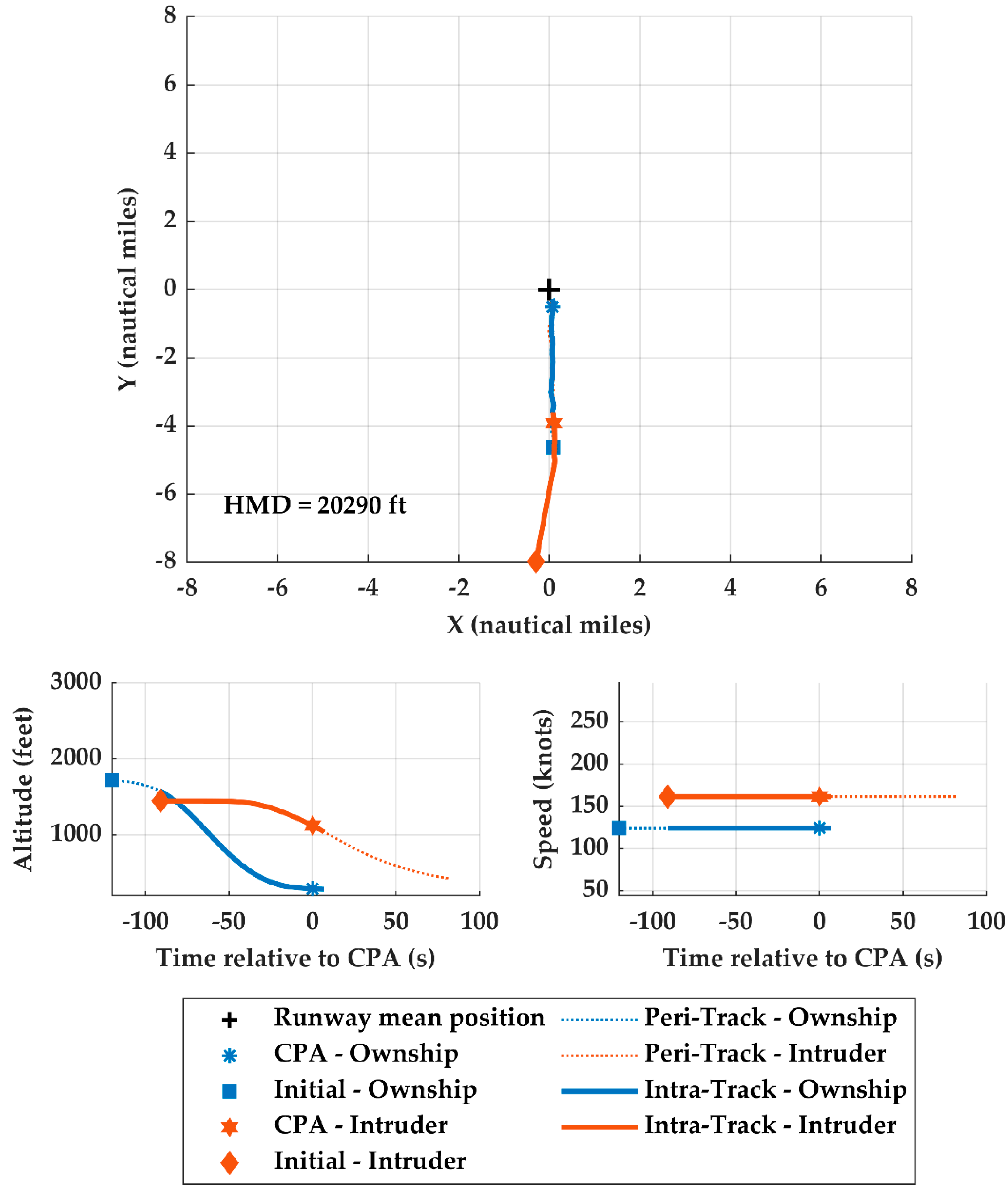
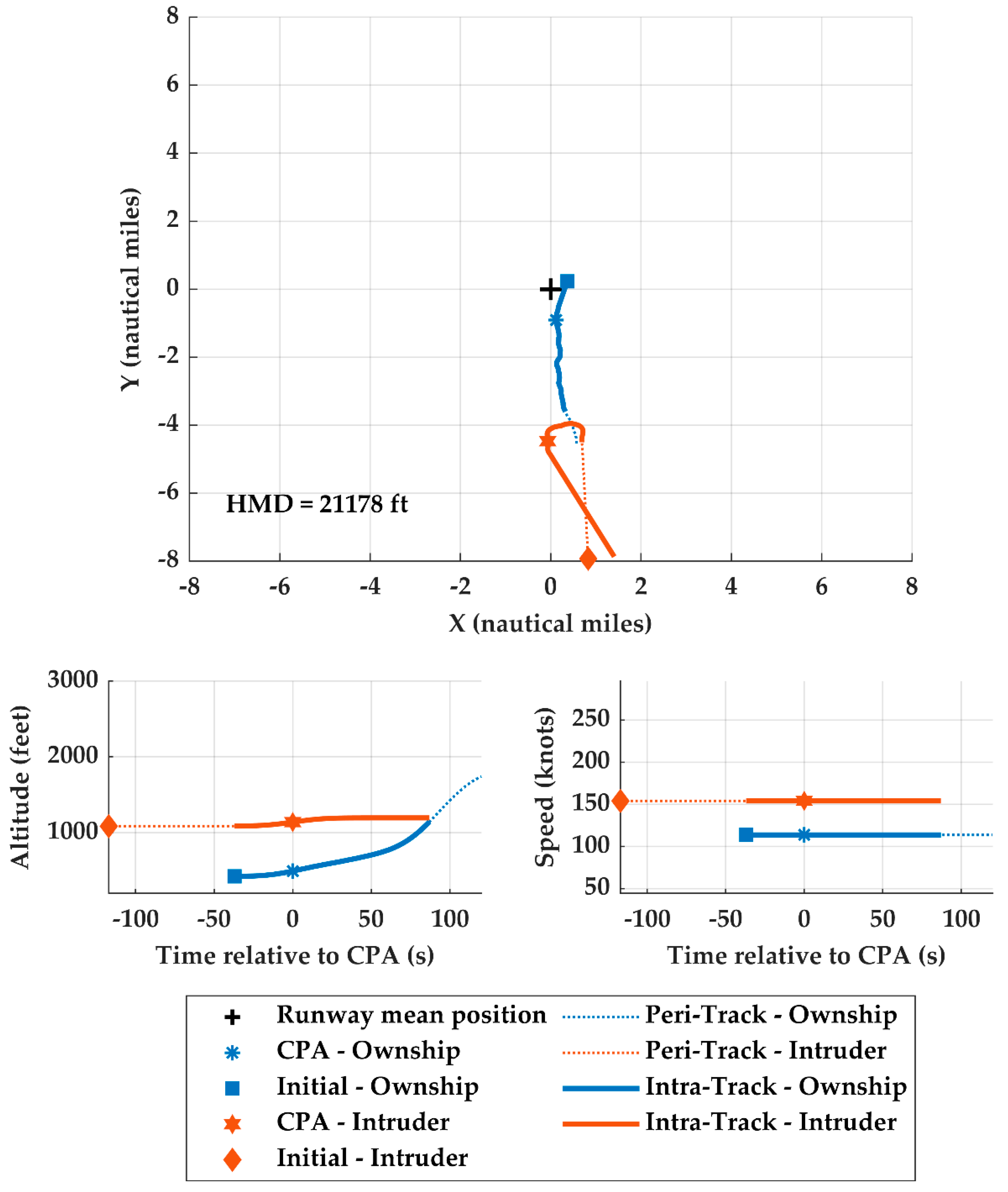
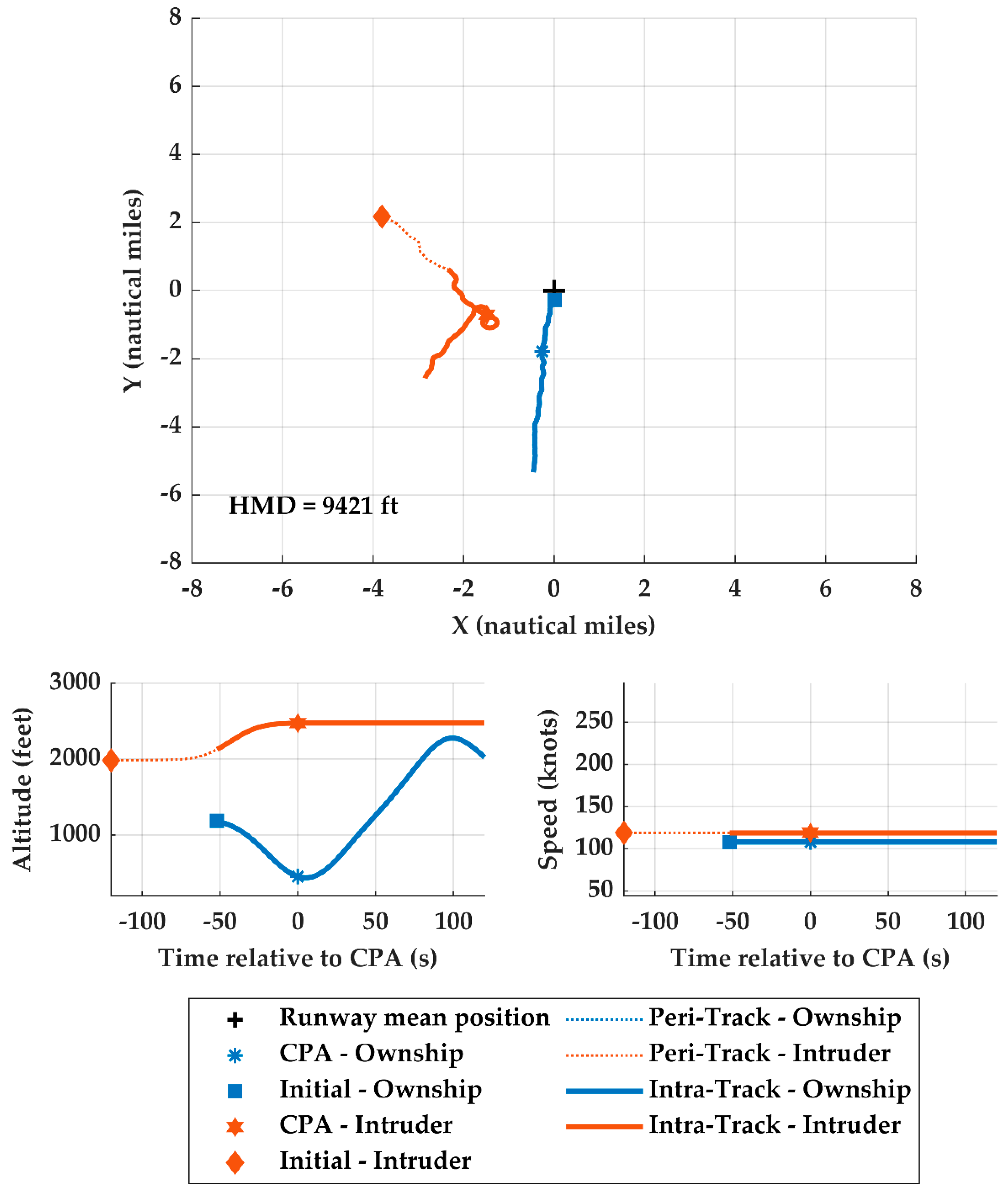
4.5. Example Nominal Encounters

Figure 24, Figure 25 and Figure 26 illustrate example encounters sampled from the model trained from terminal area radar tracks. Sampled encounters assume a generic aircraft type, and not necessarily reflective of the desired range of dynamics from Table 7. Examples are intended to highlight the advantages and disadvantages of the model and rejection sampling approach to create encounters. In all the examples, the runway is oriented parallel to the y-axis. Tracks are illustrated as peri- or intra-. Track updates when only one aircraft is simulated at the timestep are noted as peri- while track updates when both aircraft are simulated are intra-.

4.5.1. Sampled Nominal Landing Encounter

Figure 24 illustrates a sampled encounter where both aircraft are landing. While ownship must land straight, the intruder happens to also land straight but is not required to do so. The encounter starts at 120 s prior to CPA with only the ownship track simulated until 91 s prior to CPA when the intruder track is initialized approximately 8 nautical miles away from the runway. The ownship track ends shortly after CPA because it had a low enough altitude and close enough to the runway such that the tracks end. The intruder aircraft continues to be simulated until it ends at 82 s after CPA.
This illustrate how model structure influences the simulated kinematics. Both vertical rate and speed are estimated from track updates with vertical rate derived from the difference between altitude reports and speed based on distance and bearing from the runway. Altitude is a temporal variable with (t) and (t + 1) variables in the trajectory model but distance and bearing from the runway are not. Consequently, vertical rate is better modeled and more realistic. We rarely observe speed changes in sampled tracks.

4.5.2. Sampled Encounter with Transiting Intruders

Figure 25 illustrates an ownship taking off, like Figure 24, but has an intruder transiting through the airspace. Ownship exhibits similar features as in the previous examples with minimal heading changes, a reasonable vertical rate, and a constant speed. Since the coordinate system is centered on the assumed runway mean position, rather than an end of a runway, a track can be initialized anywhere near the origin, not necessarily on the y-axis. More importantly, this example illustrates how a transiting intruder behaves differently than one taking off or landing. The intruder has a relatively constant altitude, more heading changes, and flies relatively farther away from the runway.

4.5.3. Sampled Encounter Idiosyncrasies

Figure 26 illustrates an ownship taking off and an intruder transiting the airspace. The intruder maintains a relatively higher altitude and more lateral movement. Similar to the previous examples, ownship has minimal heading changes but exhibits an interesting altitude and vertical rate behavior. The ownship has an initial position within 2.5 nautical miles of the runway but at an altitude greater than 750 feet. The previously described rejection sampling criteria is that at least one track update within 2.5 nautical miles of the runway must have an altitude of 750 feet or less and given that ownship is taking off, a sufficient number of track updates need to have a vertical rate of at least 300 feet per minute. Since the ownship immediately descends to an altitude below 750 feet, it satisfied the altitude criteria when near the runway. As the track climbs after CPA, it then also satisfied the vertical rate criteria. This example illustrates an advantage of using encounter models to support Monte Carlo simulations for safety evaluations. In practice, not all takeoffs have a smooth vertical ascent and not all landings have smooth descents. This encounter also is not physically impossible. While encounters like this, it is reasonable to include them in safety assessments because they stress DAA systems in novel ways.

5. Sampled Encounter Dataset

To characterize the model samples at scale, one million encounters were generated each from models trained on the terminal radar tracks and OpenSky Network. Ownship used “RTCA228-A1” dynamic constraints while the intruder used the “generic” constraints. For each of these million encounters, there was a uniform distribution over airspace class, ownship intent, and intruder intent. The encounters were simulated using a basic 6 degrees-of-freedom dynamics model in the DEGAS simulation environment [26]. We characterized the encounter sets based on aircraft kinematic states at CPA and the horizontal miss distance (HMD) and vertical miss distance (VMD) at CPA. Distributions were compared between the different models to characterize if the different training datasets led to different sampled encounters. Ultimately, training data sources have different biases and assumptions, so generating encounter sets using both modeled improved the robustness of the final simulation results.

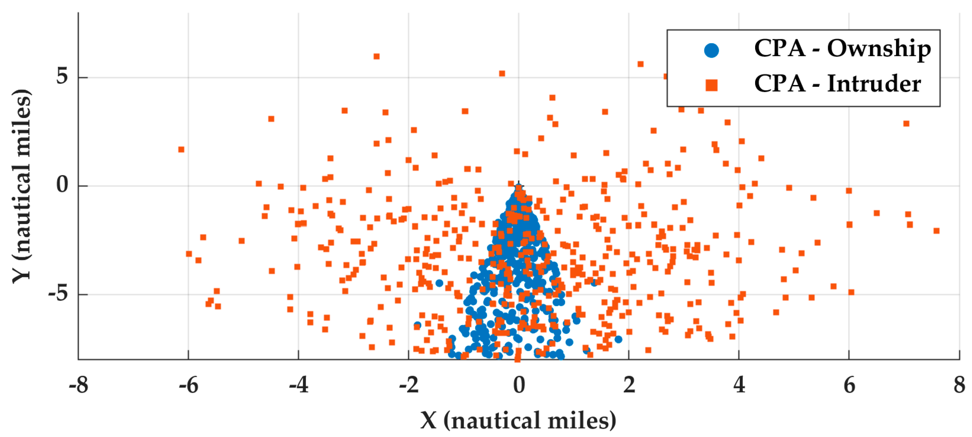
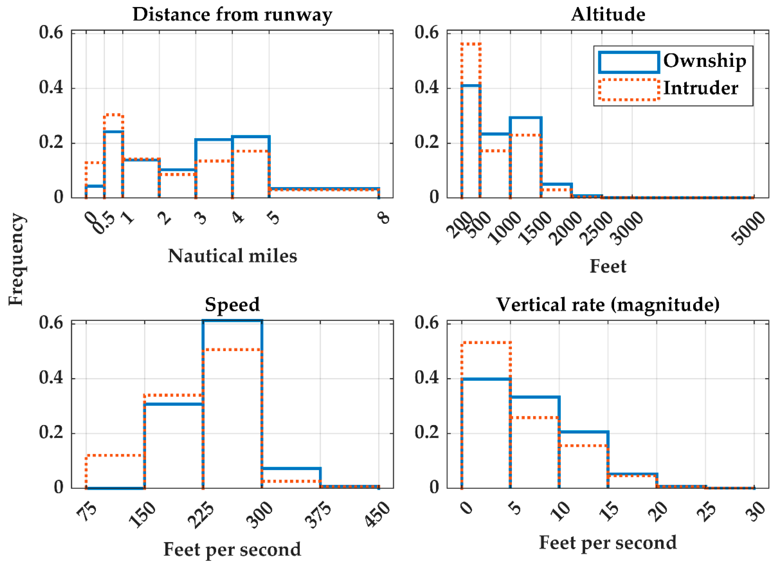
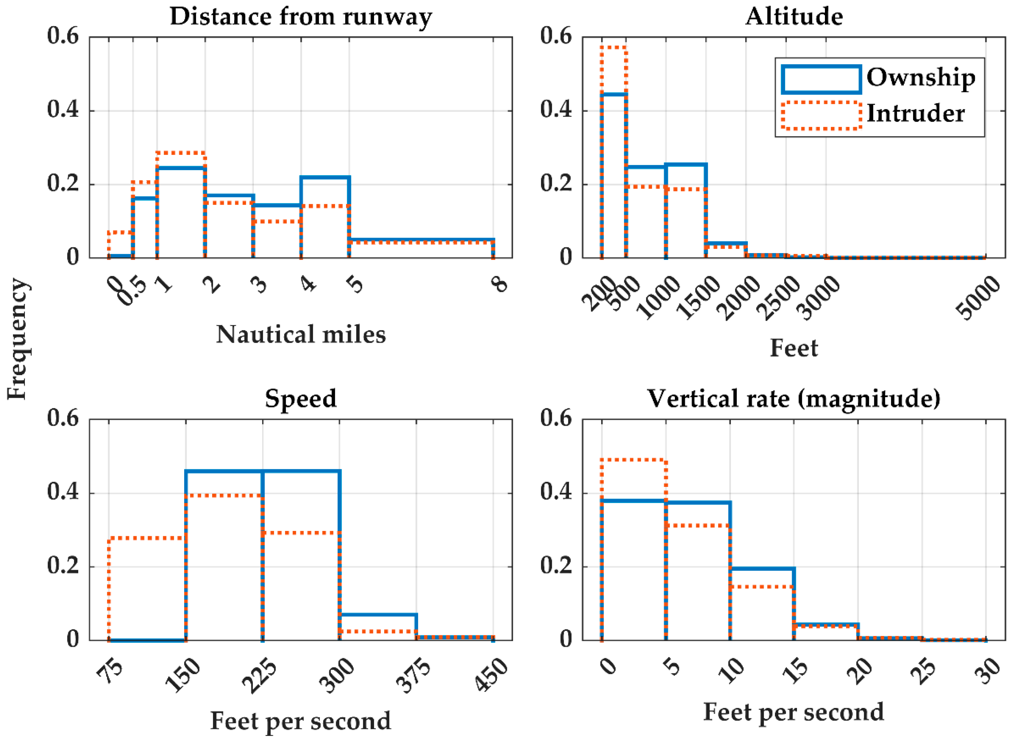
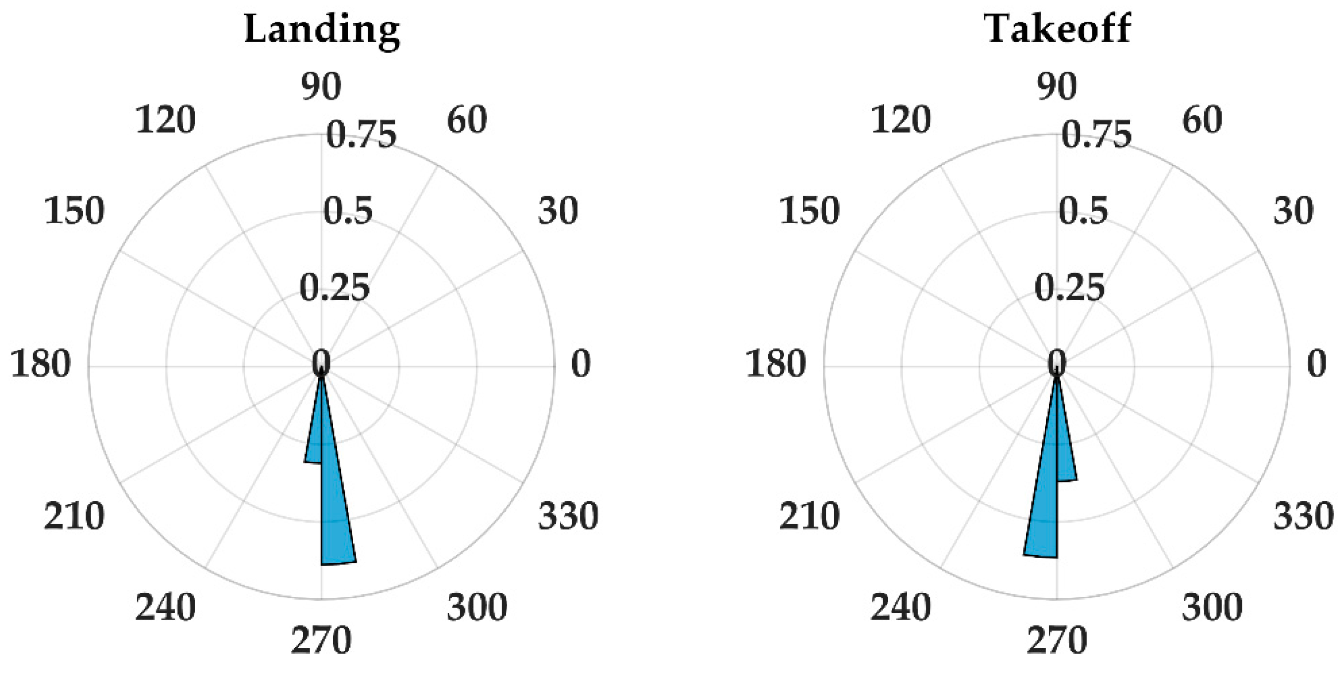
5.1. Kinematic Distributions at CPA

Figure 27 and Figure 28 provide the distributions for distance from the runway, altitude, speed, and vertical rate for ownship and intruder at CPA. Figure 27 was generated using the model trained using the terminal area radar tracks while Figure 28 used the OpenSky Network-based model. Histogram bins are based on the bins used by the encounter geometry model and may not be uniform.
Foremost, the altitude and vertical rate magnitude distributions were similar between the models. In general, the intruder was at lower altitude than the ownship at CPA, with both aircraft at 1500 feet or less. Extreme vertical rates were rarely observed at CPA, with most vertical rates of 10 feet per second (600 feet per minute) or less. The distance at which CPA occurred from the runway slightly differed between the sampled encounter sets. While both encounter sets had approximately 75% of encounters within 4 nautical miles of the runway, the terminal area radar-based encounters had more encounters within one nautical mile of the runway, while the OpenSky Network-based encounters had a few more encounters at two to four nautical miles from the runway mean position For assessing DAA performance, these differences are not particularly impactful because the DAA system is more influenced by the kinematics of which altitude and vertical rate had unimportant differences but there was a notable difference in the speed distributions.
For the terminal radar-based encounters, approximately 60% of encounters had ownship flying between 225 to 300 feet per second at CPA, while only 46% of OpenSky Network-based encounters had ownship at that speed at CPA. Additionally, only approximately 12% of intruders had a speed of 75 to 150 feet per second at CPA with the terminal radar-based encounters, compared to nearly 28% of the other encounter set. Speeds greater than 300 feet per second (178 knots) at CPA were infrequently observed in approximately 7% of encounters in both sets.
Upon review of the encounters, we have a couple hypothesis to explain the differences in the speed distributions. Principally, aircraft type of fixed-wing or rotorcraft can be identified when training with the OpenSky Network-based model but not when using the terminal area radars. For the uncorrelated encounter models, we have observed models trained solely using observations of rotorcraft will have a speed distribution slower than models trained using solely fixed-wing aircraft [7]. An uncorrelated rotorcraft-based model also has a relatively slower speed distribution than a model trained using heterogenous mix of aircraft types. We hypothesized a similar trend is occurring with the terminal model, where the OpenSky Network-based model can leverage the aircraft type information and generate tracks that are more representative of relatively slower moving aircraft. An inspection of the model distributions given an aircraft type of rotorcraft support this hypothesis. Additionally, due to ADS-B transponder equipage mandates, it is possible that more rotorcraft or general aviation fixed-wing single engine were equipped with transponders in 2018 than in 2015 when the terminal area radar dataset was curated. The models also inherently were trained based on different compositions of aircraft types, with the speed distributions reflecting these different compositions.

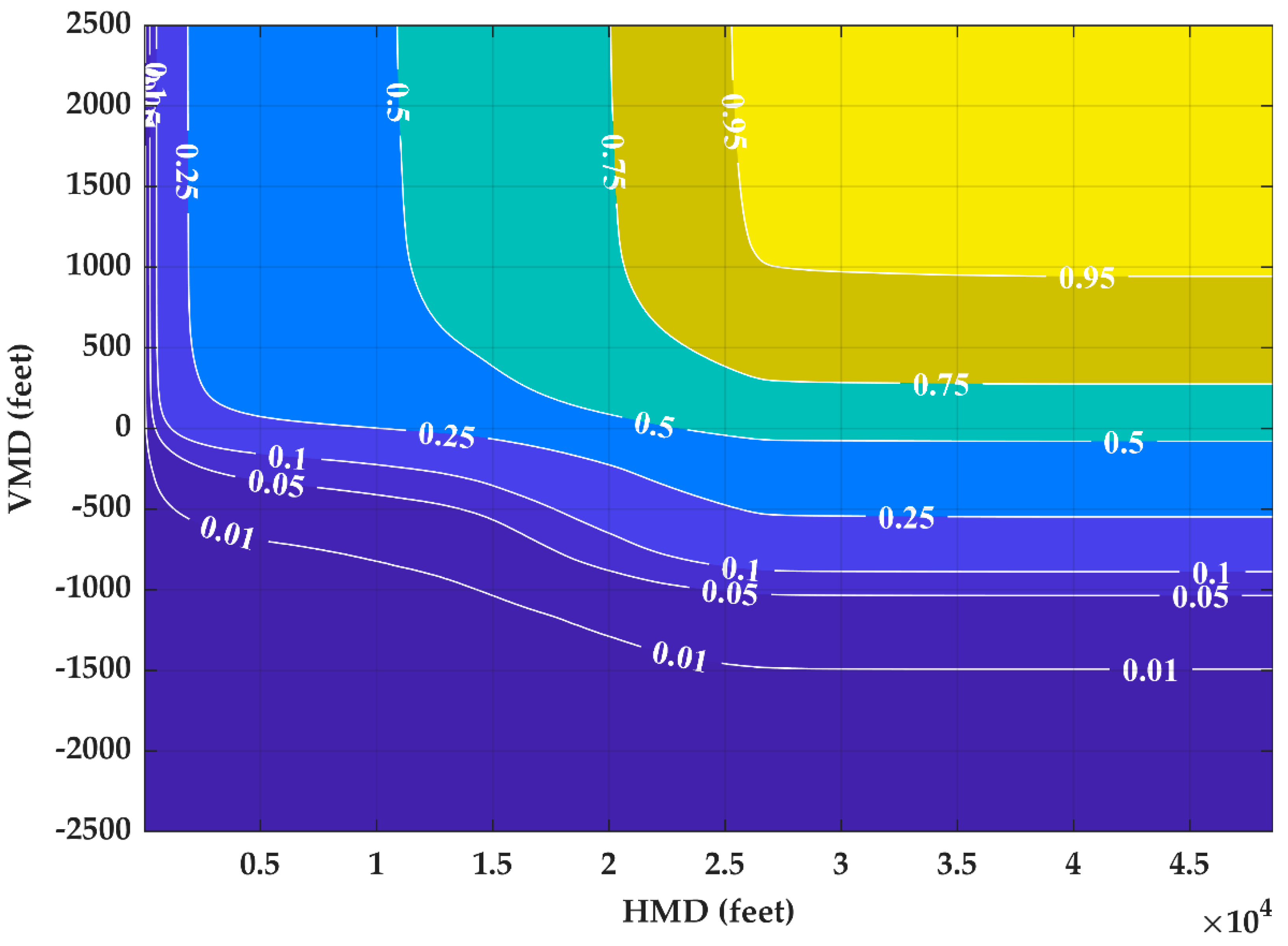
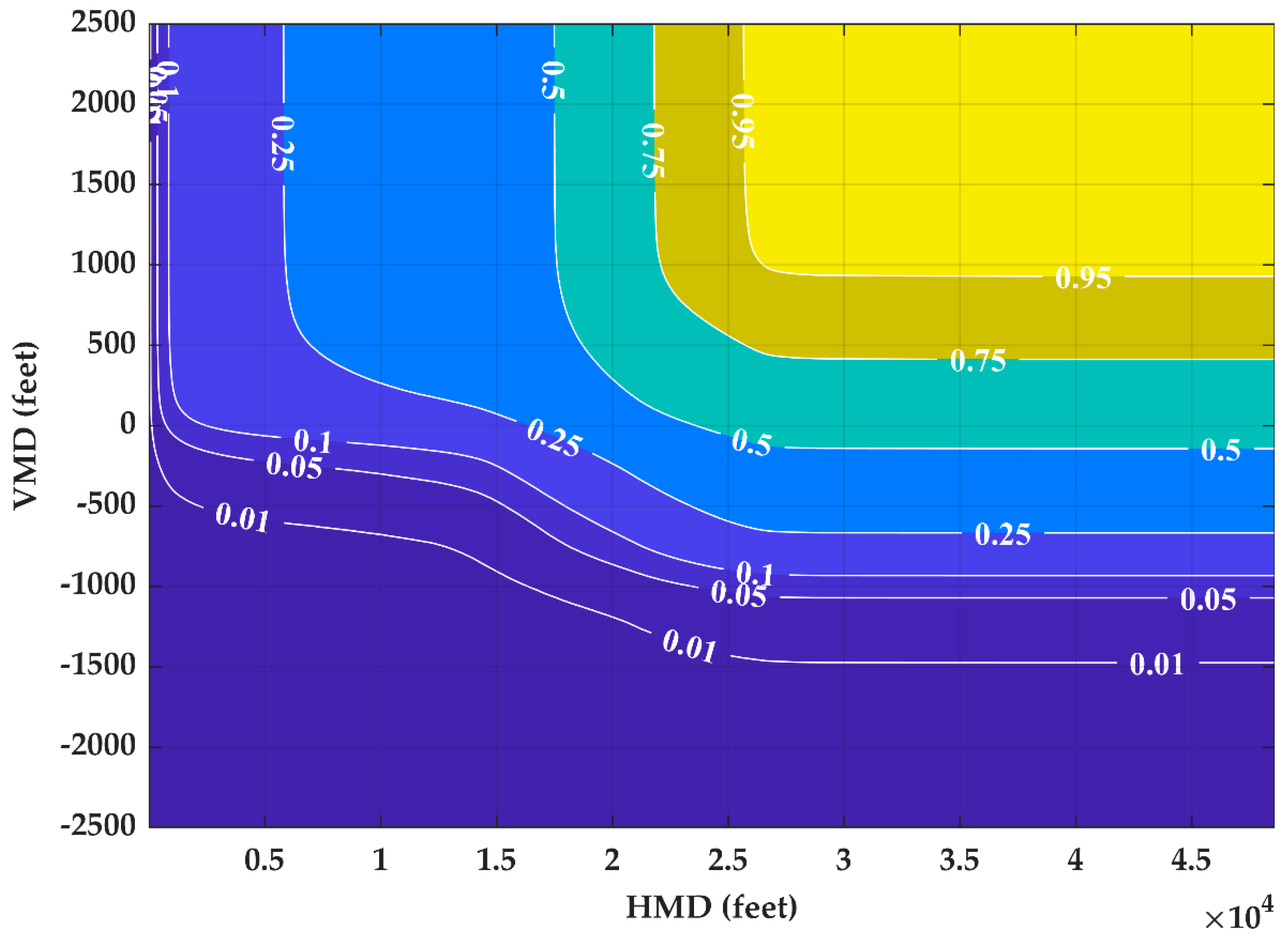
5.2. Horizontal and Vertical Miss Distance Distributions

While independent aircraft speeds are important in characterizing an encounter, the closing speed between aircraft significantly influences the risk of a collision given an encounter and subsequently the HMD and VMD at CPA. The separation between aircraft is also based on other kinematic variables as well, such as relative heading between aircraft, aircraft turn rate, altitude, and vertical rate. Accordingly, Figure 29 and Figure 30 visualize the HMD and VMD distributions as two-dimensional CDF contour plots for each encounter set; while specific values from these distributions are summarized in Table 8. The differences between these distributions are more pronounced at smaller HMD and VMD values and that as HMD and VMD at CPA increases, the distributions between the two encounter sets become more similar.
A positive VMD is indicative of the intruder above ownship and a negative VMD is when the ownship was above the intruder. Figure 29 indicates that 25% of encounters sampled from the terminal area radar trained model, had an HMD of 7000 feet or less and a VMD of 500 feet or less at CPA. Whereas 40% of encounters sampled from the OpenSky Network-based model satisfied these HMD and VMD thresholds.
Regardless of the model, majority of encounters had a CPA where the intruder was above the ownship. This can be attributed to transiting intruders which tend to have higher relative altitudes and the glide slope constraints on the ownship. Majority of encounters had a HMD and VMD greater than 2200 and 450 feet, respectively, at CPA. This combination of HMD and VMD are notable as it a separation metric used by RTCA SC-228 [27,28,29] and similar to separation criteria used by a different DAA standard published by ASTM F38 [30]. As the OpenSky Network-based model had 25% of encounters with a HMD and VMD of this or less, that encounter set was slightly more stressing to the DAA system and had encounters to estimate safety metrics based on that separation.

6. Discussion

This section critically summarizes the model and discusses potential future work. As of December 2021, model development is ongoing.

6.1. Accomplishments

Using a classical Bayesian network to model where CPA occurred was shown to be practical and scalable, whereas many of the issues can be attributed to propagating tracks over the duration of the encounter. We also demonstrated the viability of a clustering approach to identify encounters based on assumptions of airport design, approach and departure routes, and aviation heuristics. When parallelizing across multiple processors on the LLSC, the approach identified a sufficient set of encounters for model training.
Regarding the use of the model for safety analyses, aircraft tracks were often initialized multiple nautical miles away from the runway and with faster airspeeds than associated with landings of rotorcraft, fixed-wing single-engine or smaller fixed-wing multi-engine aircraft. However, as discussed in Section 3.3.1, the modeled speeds at CPA were reasonable. There was no indication that aircraft were modeled with speeds slower than anticipated nor with unreasonably fast speeds at low altitudes. Collision risk increases with aircraft speed because closing speed also increases, which reduces the time required to loss of separation between aircraft. This was previously assessed for uncorrelated encounters with smaller drones [31]. Given there exists some relationship between closing speed and risk, we assumed that the sampled encounters likely did not underestimate risk because the sampled encounters were presumed to not be slower than reality. Collision risk is not solely dependent on closing speed and there are other variables, many of which are encoded in the model itself. So, while modeled aircraft are not slowing down as they fly closer to the runway, additional validation is required to assess if the encounters slightly overestimated the risk due to the higher than expected speeds. Assuming fixed-wing aircraft have a minimum stall speed of 75–100 feet per second, we hypothesize that tracks could experience a speed change up to 85 feet per second over the course of an encounter in an improved model. Additional information may be found in the websites listed under Supplementary Materials.

6.2. Future Work

Model development will focus on improving how aircraft move through the airspace with respect the runway, rather than identifying where CPA or if an encounter was observed. Potential near-term future work includes aggregating the trajectory models into a one or two trajectory model with additional parent variables to denote if an aircraft is the ownship or intruder; or specifying additional, more specific intents such as “landing-straight,” or “landing-any.” Future work could also explore training a model using a hidden semi-Markov model, like Mahoubi and Kochenderfer [18], or with longer timesteps, such that, for example, track updates are sampled every ten instead of every one second. However, neither of these proposed developments would address issue of sampled speeds generally remaining constant.
Additionally, track classification for training and the model structure can be improved to better distinguish and model different track intents. Specifically, the current intruder intent of “transiting” can be too vague and likely insufficiently captures behavior tailored to terminal VFR or helicopter routes.
It was insightful that vertical rate estimated from a temporal variable, altitude, was a better model than speed, which was not estimate from a temporal variable. While we could prototype modifying the trajectory model such that distance and bearing from the runway are temporal variables, the current Dynamic Bayesian network structure is reliant upon discretized variables, which could produce similar intra-bin sampling issues.
One potential approach is to use aggregate or relative variables, instead of absolute variables in the model structure. Speed and vertical rate are currently absolute variables that models the absolute kinematics of the aircraft. An example aggregate variable would be the sum of aircraft speeds or the sum of vertical rates; while a potential relative variable would be the relative speed difference between the ownship and intruder. Using absolute, aggregate, and relative variables in combination could be memory efficient and better model the combinatorial state space of different aircraft kinematics. The use of aggregate states yielded promising results when previously exploring aircraft avoidance Markov Decision Processes (MDP)s [32].
Another approach similar to Mahboubi and Kochenderfer [18] could be prototyped where tracks can be classified by the probability of an aircraft transitioning from one navigation goal to the next. While Mahboubi and Kochenderfer used Turning Points as a navigation goal, goals could also be formulated origin and destination (O-D) pairs. O-D pairs have been used to model potential air taxi traffic between locations, with O-D pairs enabling models to assess various operational constraints between different structured routes [33]. Mahboubi and Kochenderfer modeled aircraft navigation between stochastic O-D pairs, the parameters and nodes of the models were hand engineered based on a nominal traffic pattern, while demonstrating they could be learned from observations.
We hypothesize that instead of a network based on specific phases of a terminal operation, such as states associated with a 45 degree entry into a downwind, turn onto base, and a turn into final before landing. Using the existing or modified model structure, Dynamic Bayesian Network(s) could be trained for each state. For example, consider a terminal environment with a single runway and VFR route. The VFR route could be composed of multiple waypoints but the proposed model would represent the entire VFR route as a single state. Similar to the cluster approach described in Section 2.3, we could identify tracks with a VFR route state. Subsequently, states associated with landing or taking off from the ends of the runway would have their own states. Given this state classification, we could train models tailored to the states. Then, similar to the encounter identification approach from Section 2.4, we could identify encounters given navigational state and relative position. This should enable the model to better distinguish between an intruder flying along a VFR route with specific operating rules and assumptions and an intruder transiting through the airspace at relatively higher altitudes. Each state could have a Dynamic Bayesian network to model how aircraft operate within a state (i.e., flying along the VFR route) with a separate Bayesian network to model the transition between states. This hierarchical model would then enable modeling of both aircraft kinematics and the relative interactions between navigational states. Notwithstanding, future work will focus on improving modeled speed and various intents.
Other avenues for future work include rotorcraft track identification with techniques that do not leverage the aircraft registry, such as using an autoencoder [34] or kinematic features [35]; considerations for non-conventional aircraft, such as gliders or balloons; incorporate traffic flow management concepts [36]; or compare sampled tracks between the correlated terminal and en route models.

Supplementary Materials

Andrew Weinert, “Validating Encounter Model Assumptions and Representativeness for the Class B Environment,” 13 October 2021. https://zenodo.org/record/5539498; Andrew Weinert, Marc Brittain, Ngaire Underhill and Christine Serres, “Benchmarking the Processing of Aircraft Tracks with Triples Mode and Self-Scheduling”, 1 September 2021. https://zenodo.org/record/5338796#.YekZz3pBxPY; Andrew Weinert, “Correlated Bayesian Model of Aircraft Encounters in the Terminal Area Given a Straight Takeoff or Landing”, 6 July 2021. https://zenodo.org/record/5076477#.YekZ6XpBxPY.

Author Contributions

Conceptualization, A.W., N.U., C.S. and R.G.; data curation, A.W., N.U., C.S. and R.G.; formal analysis, A.W., N.U., C.S. and R.G.; funding acquisition, A.W. and R.G.; investigation, A.W., N.U., C.S. and R.G.; methodology, A.W., N.U., C.S. and R.G.; project administration, A.W. and R.G.; software, A.W., N.U., C.S. and R.G.; supervision, A.W. and R.G.; validation, A.W., N.U. and C.S.; visualization, A.W.; writing—original draft, A.W., N.U., C.S. and R.G.; writing—review and editing, A.W. All authors have read and agreed to the published version of the manuscript.

Funding

Distribution Statement A. Approved for public release. Distribution is unlimited. This material is based upon work supported by the Federal Aviation Administration under Air Force Contract No. FA8702-15-D-0001. Any opinions, findings, conclusions or recommendations expressed in this material are those of the author(s) and do not necessarily reflect the views of the Federal Aviation Administration. Delivered to the U.S. Government with Unlimited Rights, as defined in DFARS Part 252.227-7013 or 7014 (February 2014). Notwithstanding any copyright notice, U.S. Government rights in this work are defined by DFARS 252.227-7013 or DFARS 252.227-7014 as detailed above. Use of this work other than as specifically authorized by the U.S. Government may violate any copyrights that exist in this work.

Institutional Review Board Statement

Not applicable.

Informed Consent Statement

Not applicable.

Data Availability Statement

Acknowledgments

The authors greatly appreciate the support provided by Sabrina Saunders-Hodge and Deepak Chauhan from the Federal Aviation Administration. The authors wish to acknowledge the support of their colleagues, Rodney Cole and Matthew Edwards. The authors also acknowledge the MIT Lincoln Laboratory Supercomputing Center for providing high performance computing resources that have contributed to the research results reported within this paper.

Conflicts of Interest

The authors declare no conflict of interest. The funders had a role in the decision to publish the results.

Appendix A. Datasets of Aircraft Tracks

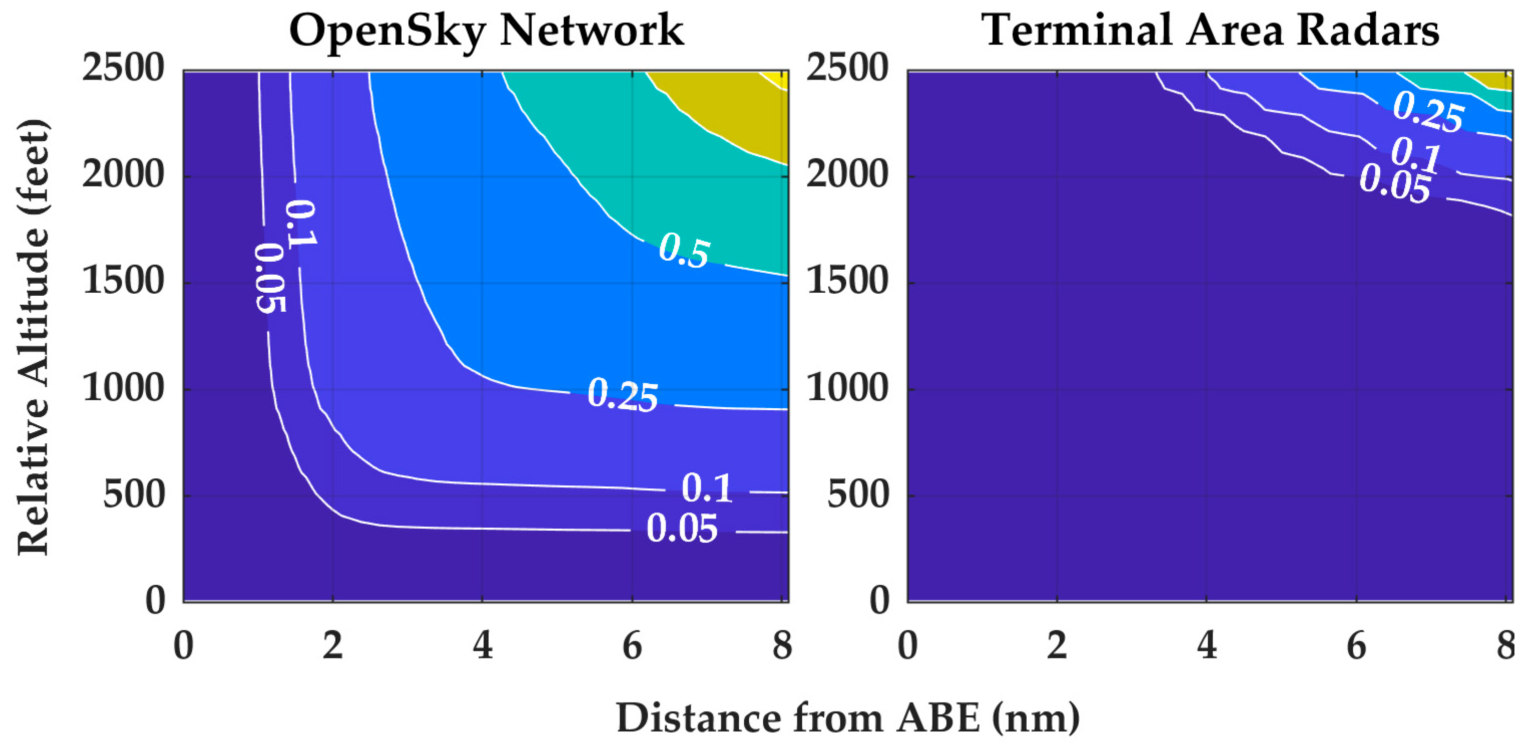
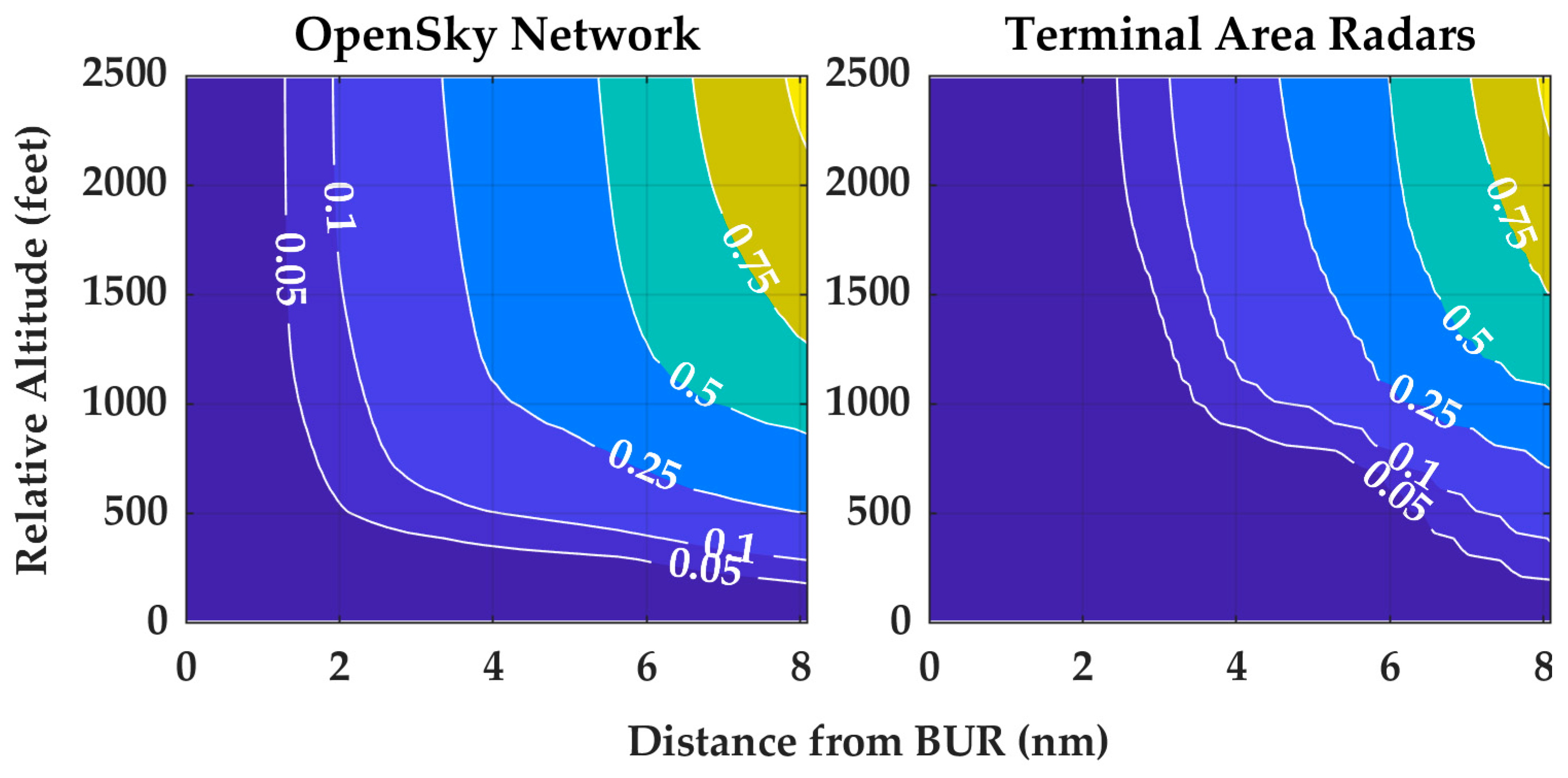
Appendix A.1. OpenSky Network

Observations of crewed aircraft were sourced from the OpenSky Network [15], a community network of ground-based sensors that observe aircraft equipped with Automatic Dependent Surveillance-Broadcast (ADS-B) Out. The OpenSky Network offers a historical database and we developed and publicly released the software, em-download-opensky [37], to generate queries based on AGL altitude, location of airports, airspace class, and time zones. Using this software, we generated 136,884 queries for 196 days across 695 bounding boxes across Class B, C, and D airspace across the United States. Temporally, we queried for the first 14 days of each month from January 2019 through February 2020. This time window was largely unaffected by the COVID-19 pandemic, as the Schengen Area travel ban did not take effect until March 2020 [38].
Prior to model training, the OpenSky Network data were (1) parsed and organized; (2) archived; and (3) processed and interpolated into track segments [39]. Processing included removing track segments with less than ten observations; calculating the above ground level altitude was calculated; identifying airspace class; and estimating dynamic rates (e.g., vertical rate) were calculated. Once processed, track segments were ready for model training. For details on how this dataset was curated and processed, please see [16] where this dataset is referred to as the aerodrome dataset.
The aerodromes dataset differed from the Mondays dataset, that was curated from the OpenSky Network to train the recent uncorrelated encounter models [16]. The Mondays dataset was curated from OpenSky Networks from 104 Mondays spanning from 5 February 2018 to 16 November 2020; not all Mondays in this span were included. This dataset was not spatially limited to regions around airports but had a more restrictive temporal scope of just Mondays.

Appendix A.2. Terminal Area Radars

Observations of crewed aircraft were sourced from raw secondary radar reports from terminal radars (ASR-9) that participated in the TCAS RA Monitoring System (TRAMS) from January through September 2015. Radars included the ASR-9 located at MIT LL and radars associated with the following airports: KATL, KDEN, KDFW, KFLL, KHPN, KJFK, KLAS, KLAX, KOAK, KORD, KPDX, KPHL, KSDF, KSEA, KSTL. The specific radar identifiers were, respectively, Atlanta (ATL), Denver (DEN), Dallas Fort Worth (DFW), Fort Lauderdale (FLL), Westchester County (HPN), New York (JFK), Las Vegas (LAS), Las Angeles (LAX, LAXN), MIT LL (MOD), Oakland (OAK), Chicago (ORDA), Portland (PDX), Philadelphia (PHL), Phoenix (PHX), Louisville (SDF), Seattle-Tacoma (SEA), St. Louis (STL). These radars support the TCAS Operational Performance Assessment (TOPA) program that was established over a decade ago [40]. While TOPA is ongoing program, the data made available to support model development varied in quantity and temporal scope. For example, KDFW had data from January through August while KOAK only from June through August.
These radar reports provide latitude, longitude and barometric altitude for transponder-equipped aircraft within the radar’s surveillance volume. All of these radars were located within a Mode C veil, where aircraft, with few exemptions, are required to be transponder-equipped. While these radars surveil standard aviation transponders, not all surveillance information was made available to MIT LL. Specifically, the Mode S address was not included in this dataset, preventing classification of aircraft type using the approach described in [39].

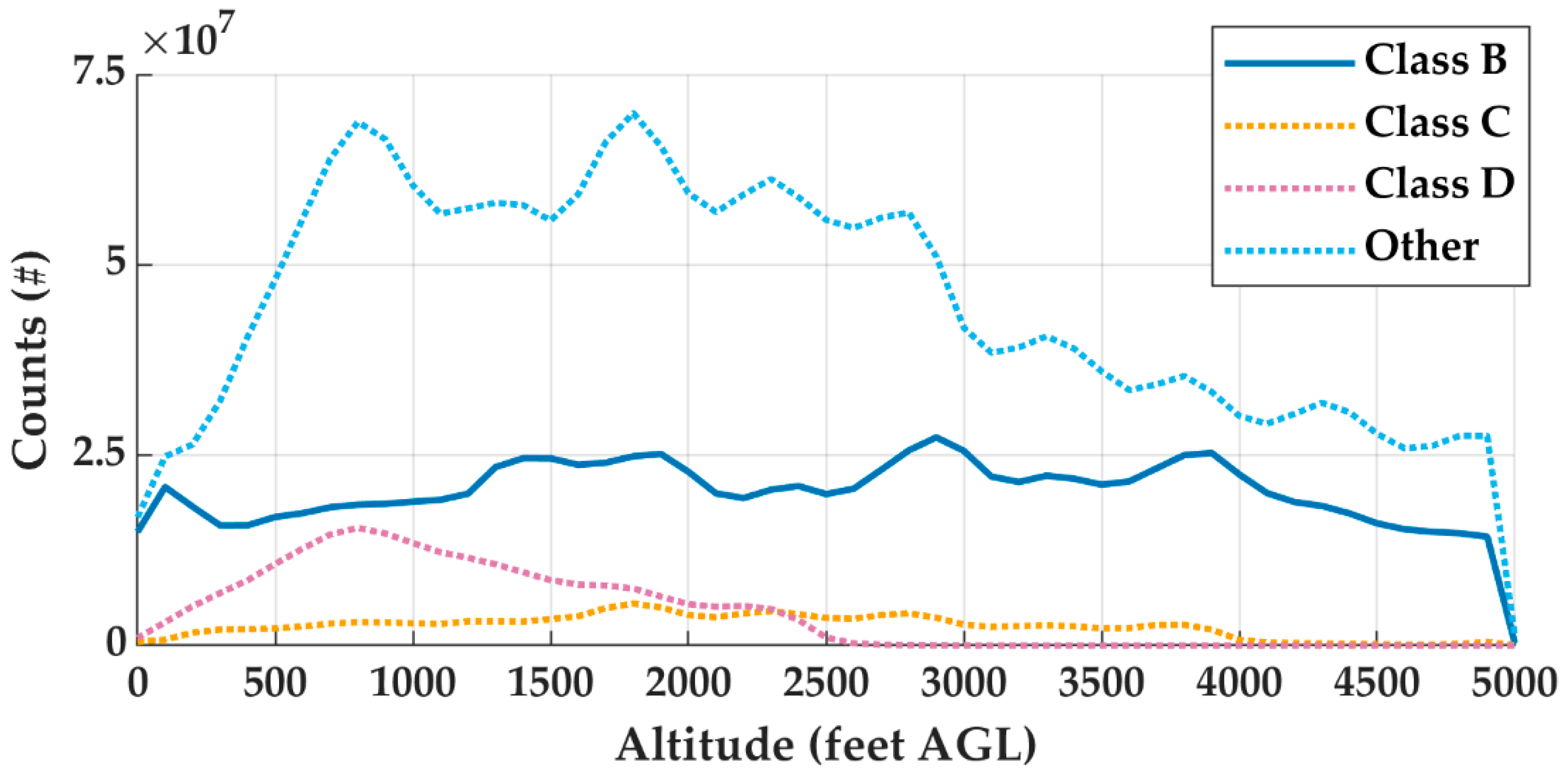
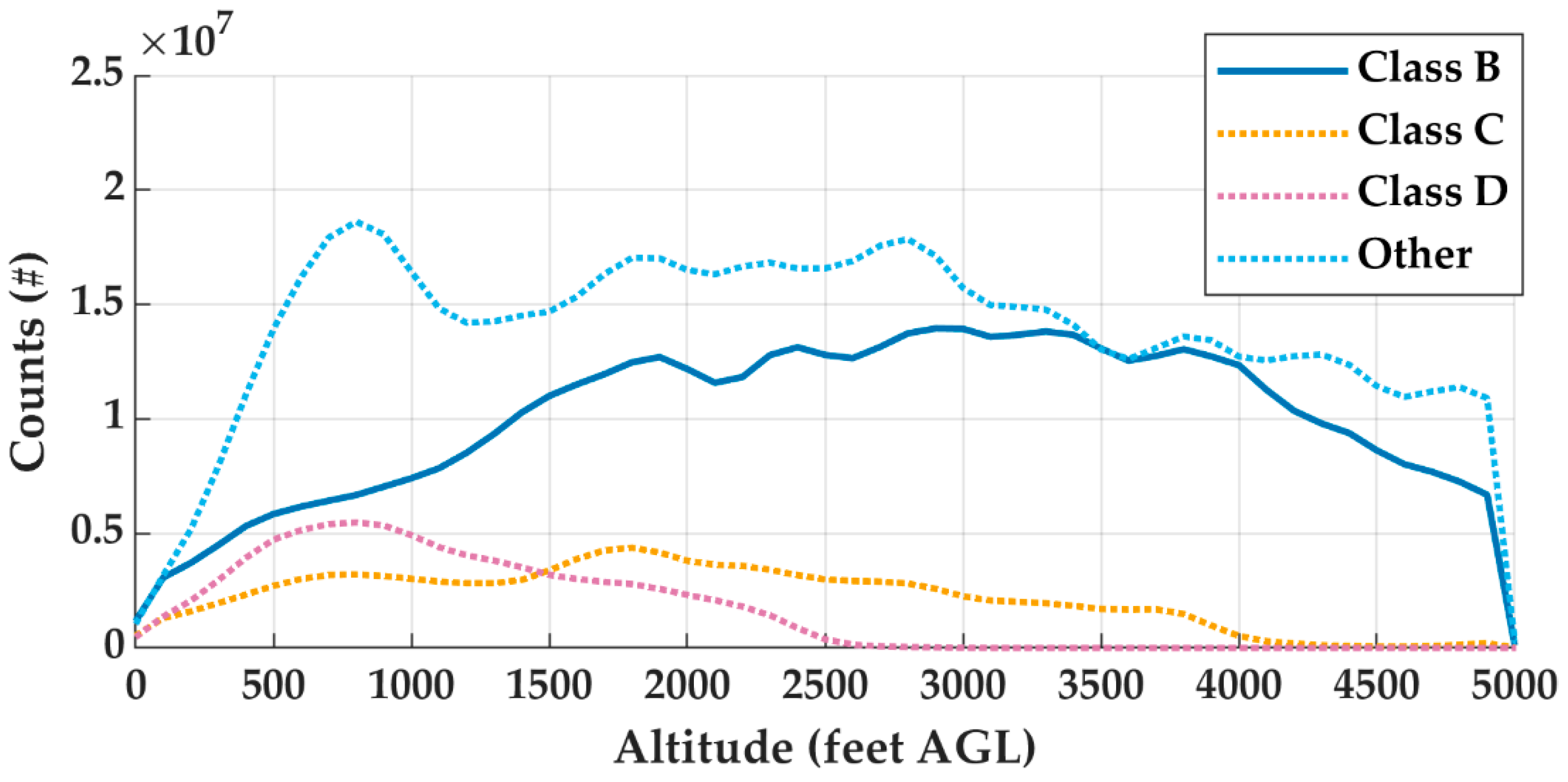
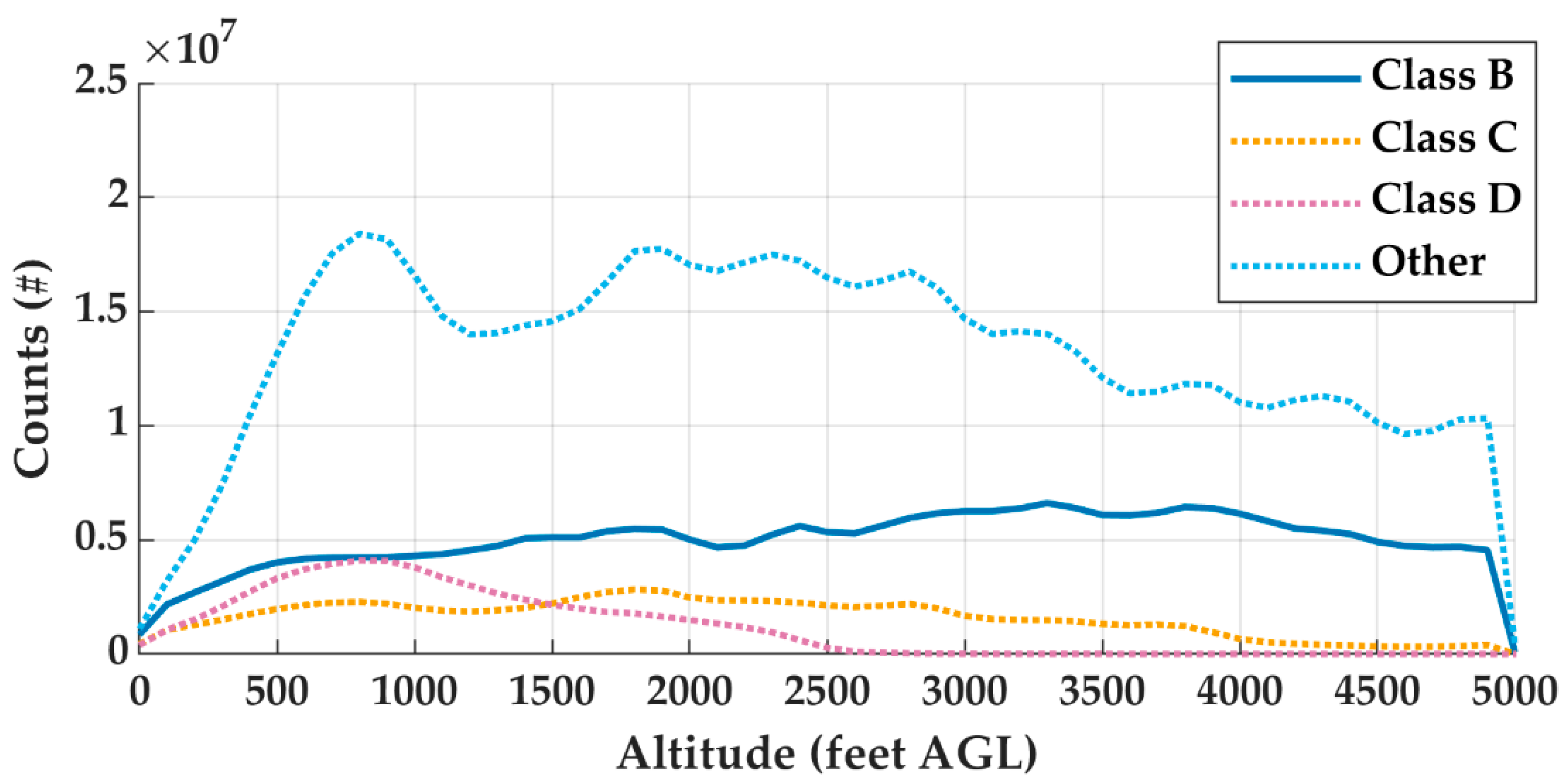
Appendix A.3. Altitude and Airspace Class Characterization

To identify potential biases in the training data, we characterized the different datasets, leveraging software and a methodology previously described in [41]. This characterization was also important in assessing if the different training datasets were similar or different and if there was a sufficient difference between datasets to warrant training a model with each dataset. For each dataset, the altitude distributions given airspace class was calculated using all latitude, longitude, and barometric altitude reports using the workflow described in [39]. Unlike [41], we did not consider the number of seats onboard the aircraft, as we lacked the metadata in the terminal area radar dataset required for that characterization. Figure A1 is for the terminal area radar dataset, Figure A2 for the OpenSky Network aerodromes dataset, and for comparison, Figure A3 is the distribution of the “Mondays” dataset used for the recent uncorrelated encounter models.
First, we observe in Figure A1, Figure A2 and Figure A3 the Class C and D distributions taper off at 2500 and 4000 feet AGL, the nominal ceilings for the respective airspace classes. Regardless of airspace class, the majority of observations were above 500 feet AGL. Note that the limit of the y-axis is greater in Figure A1 than Figure A2 and Figure A3, due to the terminal area radar dataset being significantly larger. The peak in all figures between 500 and 1000 feet was hypothesized to aircraft trying to maintain an altitude below the nominal Class E floor of 700 feet AGL or the Class G ceiling of 1200 feet AGL. The decrease in observations at 3000 feet AGL and upward can be partly attributed to behavior induced by 14 CFR § 91.159 that regulates the hemispheric flight rules and when VFR must navigate using MSL altitude. This was especially evident in the terminal area radars dataset. We also hypothesized the peak between 1500–2000 feet AGL could be attributed to general aviation cross-country operations, but no analysis was conducted to make a definitive conclusion.
Next, by comparing the figures, we observed that the terminal area radar dataset (Figure A1) had the most observations, below 1000 feet, in Class B and other airspaces, followed by the aerodromes dataset and lastly by the “Mondays” dataset. As the terminal area radars were largely co-located at Class B airports, this was expected. The aerodromes dataset had the most observations for the Class C and D airspaces. At higher altitudes, there was less of a difference between the terminal area radar and aerodrome datasets for Class B but the terminal area radars consistently had significantly more observations for the other airspace classes.
Figure A1. Altitude distributions below 5000 feet AGL for the terminal area radars dataset.
Aerospace 09 00058 g0a1
Figure A2. Altitude distributions below 5000 feet AGL for the aerodromes dataset.
Aerospace 09 00058 g0a2
Figure A3. Altitude distributions below 5000 feet AGL for the Mondays dataset used to train the OpenSky Network-based uncorrelated encounter models.
Aerospace 09 00058 g0a3
Since the model encompassed the airspace within 8 nautical miles of the airport, identified encounters can cross multiple airspaces. Generally below 1200 feet AGL, Class C and D airspaces extend 2.5–5 nautical miles from a controlled runway. Given our encounter range criteria of 4 nautical miles, an encounter could occur when one aircraft was in Class D airspace and another in other airspace. An aircraft could also transition between airspaces over the course of the 30 s encounter duration. Thus, the significantly more observations of aircraft in other airspace at low altitudes was advantageous for the terminal radar dataset. The terminal area radar dataset had the most observations for a given location, if lower altitude surveillance was available, but this dataset was also the most restricted spatially and temporally.
Furthermore, when comparing the two OpenSky Network-based datasets, the percent difference between datasets for Class E and G (other) airspace was only 4.27%, yet it was 30% or greater for the other airspace classes. These percent differences demonstrate the advantage of curating a dataset, based on areas of interest, by querying the OpenSky Network. While the “Mondays” dataset has theoretically the best spatial coverage, as all data observed in the United States is in scope for that dataset, the OpenSky Network does not have universal low-altitude coverage across the United States. The OpenSky Network has significant coverage gaps in rural or low population areas. However, these regions also typically have a low density of crewed aircraft traffic and these coverages gaps are not a significant impediment for model training. Accordingly, the wider temporal scope of the aerodromes dataset and surveillance of more types of transponders with the terminal area radar dataset results in these datasets having more observations than the “Mondays” dataset. The “Mondays” dataset also included 2018, when fewer aircraft were equipped with ADS-B and fewer sensors were participating in the OpenSky Network, and 2020 when aviation activity sharply decreased due to the COVID-19 pandemic [38].

Appendix A.4. Data per National Plan of Integrated Airport Systems

Table A1 reports the data identified as spatial filtering for select airports. For each airport, we also noted if the airport was designated as a primary airport in the 2015–2019 FAA National Plan of Integrated Airports Systems (NPIAS) [42]. Primary airports are grouped into categories of large (L), medium (M), small (S), and nonhub (N). Large hubs are those airports that each account for at least 1% total U.S. passenger enplanements; while nonhub primaries enplane less than 0.05% of all commercial passenger enplanements but have more than 10,000 annual enplanements. Medium and small hubs are grouped between large and nonhub primaries.
Table A1. Total track points after initial spatial filtering for select airports.
FAA IDClassHubOpenSky NetworkTerminal Area Radar
BOSBL10,881,93813,270,494
ABECN1,816,6702,285,593
BURCM16,789,41029,748,003
FLLCL10,342,13050,856,891
SMFCM6,876,0290
XNACS1,466,7940
ACKDN21,9340
ADSD-20,954,31568,151,579
BEDDN2,740,6646,220,588
EYWDS00
MVYDN820,6540
RNTD-21,892,54746,653,226
TTDD-5,360,10614,106,809
7N7E/G-7,968,29518,523,179
17NE/G-2,252,99513,006,900
19NE/G-5,818,46218,784,328
DDHE/G-00
As hubs increased in enplanements, we generally identified more potential tracks; although there was not a strong correlation. The quantity of data was dependent more on the surveillance source, which likely has some correlation with NPIAS categorization. For example, Addision Airport (ADS), a nonprimary national airport, had one of the largest datasets. The size of the ADS dataset, however, was due to ADS located in the vicinity of Dallas Love Field (DAL) and Dallas Fort Worth International (DFW) which are medium and large hubs, respectively. Additionally, more data were available for BED and ABE, nonhub primaries, than XNA or EYW, small hubs. These four airports all had less data identified than Oldsman Township Airport (7N7), a non-towered single-runway airport approximately 10 nautical miles from Philadelphia International.
One potential bias was due to the that the ADS-B FAA mandate was not in effect until 2020, whereas the majority of the OpenSky Network data were from 2019 and before this mandate. Today, ADS-B has also been mandated in most busy ATC controlled airspaces in the United States and there are various local, regional, and international roll-outs of ADS-B. As more aircraft equip ADS-B, we expect more encounters to be identified.

Appendix B

This appendix supplements Section 3.1 and illustrates by the distance from airport and relative altitude distributions for Lehigh Valley International (ABE), a Class C airport in Pennsylvania approximately 40 nautical miles north of Philadelphia, PA and 60 nautical miles west of Newark, NJ. Table A1 reported that the terminal radar dataset had at least 450,000 observations, within 10 nautical miles and 4000 feet of ABE, more than the OpenSky Network-based tracks. However, Figure A4 and Figure A5 illustrate that nearly all the terminal radar-based tracks are at least 15,000 feet above ABE, while the OpenSky Network had significantly better low-altitude coverage of the region. This would ultimately result in no encounters identified for model training with the terminal radar dataset while encounters were identified using the OpenSky Network-based dataset. Similar trends were exhibited with Hollywood Burbank (BUR), a Class C airport serving northern greater Las Angeles.
Figure A4. Fraction of aircraft positions relative to ABE.
Aerospace 09 00058 g0a4
Figure A5. Fraction of aircraft positions relative to BUR.
Aerospace 09 00058 g0a5

Appendix C

When identifying encounters as part of model training, all observations of aircraft transmitting any of the special transponder codes in the following Table A2 were rejected.
Table A2. Special use transponder codes not used for model training.
CodePurpose
1206VFR law enforcement, first responder by L.A., may not be in contact with ATC
1255Firefighting aircraft
1273–1275Calibration and performance monitoring equipment
1276Air defense identification zone penetration (when unable to contact ATC or aeronautical facility)
4401–4433, 4466–4477Special aircraft—sensitive unclassified
4434–4437Weather reconnaissance
4447–4452Special flight support codes
5000–5057, 5063–5077, 5400, 6100, 6400, 7501–7577DOD reserved codes only to be assigned by NORAD
5100–5300More DOD aircraft
7400Reserved for uncrewed aircraft with a lost link
7500Hijack
7600Radio failure
7601–7607, 7701–7707Allocated by the FAA for special use by law enforcement agencies
7700Emergency
7777DOD interceptor aircraft on active air defense missions -operating without ATC clearance
Furthermore, when training version 2.0, we assessed that the transponder code filtering did not have a significant impact on identifying encounters with the OpenSky Network based encounters. Without any Mode C filtering, 2428 Class D encounters were identified, while with filtering 2150 Class D encounters were identified. We did not repeat this analysis when training version 3.0.

Appendix D

Figure A6 visualizes all the ownship and intruder tracks for ABE used as training data for the trajectory propagation models when training with the OpenSky Network aerodromes model.
Figure A6. Example ownship and intruder tracks near ABE used for model training.
Aerospace 09 00058 g0a6

Appendix E

Summarized by Table A3. “Generic” limits are general limits applicable for a wide range of crewed aircraft. “RTCA228-A1” corresponds to the RTCA SC-228 assumptions for a HALE (High Altitude, Long Endurance) aircraft, “RTCA228-A2” for an assumed MALE (Medium Altitude, Long Endurance) aircraft and “RTCA228-A3” for an assumed LEPR (Low End Performance Representative) aircraft.
Of the dynamic limits, the acceleration limit was specifically based on the model structure and how trajectories are propagated. Since the trajectory models are sampled incrementally with intra-bin uniform sampling, it is possible to sample speed such that it transitions from 100 (bin 1) to 199 (bin 2) feet per second in one timestep. Since this would not be realistic, the maximum acceleration is based on the widest speed bin of 50 feet per second. This sampling criteria often results in tracks not changing speed.
Table A3. Dynamic limits when sampling encounters.
Variable (Units)GenericRTCA228-A1RTCA228-A2RTCA228-A3
Minimum speed
(feet per second)
501696868
Maximum speed
(feet per second)
506491338186
Acceleration
(feet per second2)
50505050
Maximum vertical rate
(feet per second)
100.0041.6725.008.34
Maximum turn rate
(degrees per second)
121.537
Maximum pitch
(degrees)
151515

Appendix G

This appendix overviews the initial approach of version 1.0 to identify if a runway was for taking off or landing. This approach was found to be sensitive to false positive identifications (e.g., wrong runway identified or assessed as landing but actually transiting). The criteria were tuned to minimize such false positives at the expense of excluding some otherwise relevant trajectories (i.e., false negatives). In response, the approach described in Section 2 was developed to reduce misidentifications, enhance the robustness and improve scalability.
Each trajectory was separately assessed for landing and for takeoff, so it can be tagged as one or the other, both, or neither. The procedure for both takeoff runway and landing runway identification entails transforming the latitude/longitude trajectory into a Cartesian coordinate frame centered on each candidate runway.
For takeoffs, the assessment is limited to the first 30 s of trajectory data. That trajectory segment is assessed against the following:
  • Trajectory segment include altitude below 1500 feet (relative to runway elevation);
  • The segment is generally increasing in altitude;
  • The ground track is aligned within 45° of the runway; and
  • The segment includes positive points on the along-runway axis that are within 4000 feet of the runway laterally.
If no runways satisfy these criteria, the trajectory is not a takeoff. (Conceivably some takeoff trajectories will be missed if they begin at the defined edge of the terminal area, land, and immediately take off again.) If a single runway satisfies the criteria, the trajectory is marked as a takeoff from that runway. If multiple runways satisfy the criteria, the trajectory is marked as a takeoff from the runway with threshold closest in ground range to the initial point on the trajectory.
For landings, a similar procedure is followed. The assessment uses the final 30 s trajectory data, which must satisfy the following criteria:
  • Includes altitudes below 1500 feet (relative to runway elevation);
  • Ground track is aligned within 35° of runway; and
  • Includes negative points on the along-runway ways that are within 4000 feet of the runway laterally.
As for takeoffs, if multiple runways satisfy the criteria, the runway with threshold closest in ground range to the final point of the trajectory segment is identified as the landing runway. Note that this procedure likewise will miss the scenario outlined above where the landing and takeoff occur in the middle of the trajectory. Both assessments neglect any events in the middle of the trajectory and do not assess, for example, intermediate landings and takeoffs in trajectories with multiple go-arounds.
Any landing trajectories are also assessed for using a straight-in approach, which require that the aircraft make no turns after passing the Final Approach Fix, which is different for every airfield but typically four to five miles from the runway. This criterion is simplified to whether the trajectory passes within one nautical mile laterally when it is at four nautical miles along the negative along-runway axis.
Finally, encounters are identified amongst the landing and taking off trajectories. To be identified as such, one track must be a straight-in landing (the surrogate uncrewed aircraft) and the second track must be a landing (either straight-in or otherwise) and/or takeoff.

References

  1. RTCA. DO-365—Minimum Operational Performance Standards (MOPS) for Detect and Avoid (DAA) Systems; RTCA: Washington, DC, USA, 2017. [Google Scholar]
  2. International Civil Aviation Organization. Global Air Traffic Management Operational Concept; International Civil Aviation Organization: Montreal, QC, Canada, 2005. [Google Scholar]
  3. Espindle, L.P.; Griffith, J.D.; Kuchar, J.K. Safety Analysis of Upgrading to TCAS Version 7.1 Using the 2008 U.S. Correlated Encounter Model; Massachusetts Institute of Technology, Lincoln Laboratory: Lexington, MA, USA, 2009. [Google Scholar]
  4. Edwards, M.W.; Kochendedrfer, M.J.; Kuchar, J.K.; Espindle, L.P. Encounter Models for Unconventional Aircraft, Version 1.0; Project Report ATC-348; Massachusetts Institute of Technology, Lincoln Laboratory: Lexington, MA, USA, 2009. [Google Scholar]
  5. Kochenderfer, M.J.; Edwards, M.W.M.; Espindle, L.P.; Kuchar, J.K.; Griffith, J.D. Airspace Encounter Models for Estimating Collision Risk. J. Guid. Control Dyn. 2010, 33, 487–499. [Google Scholar] [CrossRef]
  6. Weinert, A.J.; Harkleroad, E.P.; Griffith, J.D.; Edwards, M.W.; Kochenderfer, M.J. Uncorrelated Encounter Model of the National Airspace System Version 2.0; Project Report ATC-404; Massachusetts Institute of Technology, Lincoln Laboratory: Lexington, MA, USA, 2013. [Google Scholar]
  7. Underhill, N.; Weinert, A. Applicability and Surrogacy of Uncorrelated Airspace Encounter Models at Low Altitudes. J. Air Transp. 2021, 29, 1–5. [Google Scholar] [CrossRef]
  8. Weinert, A. Airspace-Encounter-Models/Em-Model-Manned-Bayes: October 2021; Zenodo: 2021. Available online: https://doi.org/10.5281/zenodo.5544340 (accessed on 5 November 2020).
  9. Kochenderfer, M.J.; Espindle, L.P.; Kuchar, J.K.; Griffith, J.D. Correlated Encounter Model for Cooperative Aircraft in the National Airspace System; Project Report ATC-344; Massachusetts Institute of Technology, Lincoln Laboratory: Lexington, MA, USA, 2008. [Google Scholar]
  10. Underhill, N.; Harkleroad, E.; Guendel, R.; Weinert, A.; Maki, D.; Edwards, M. Correlated Encounter Model for Cooperative Aircraft in the National Airspace System; Version 2.0; Project Report ATC-440; Massachusetts Institute Technology Lincoln Laboratory: Lexington, MA, USA, 2018; Available online: https://apps.dtic.mil/docs/citations/AD1051496 (accessed on 16 January 2019).
  11. RTCA. Terms of Reference RTCA Special Committee 228: Minimum Performance Standards for Unmanned Aircraft Systems (Rev 10); RTCA: Washington, DC, USA, 2020. [Google Scholar]
  12. Ghatas, R.W.; Jack, D.P.; Tsakpinis, D.; Vincent, M.J.; Sturdy, J.L.; Munoz, C.A.; Hoffler, K.D.; Dutle, A.M.; Myer, R.R.; Dehaven, A.M.; et al. Unmanned Aircraft Systems Minimum Operations Performance Standards End-to-End Verification and Validation (E2-V2) Simulation; Technical Report NASA/TM-2017-219598; NASA Langley Research Center: Hampton, VA, USA, 2017. Available online: https://ntrs.nasa.gov/search.jsp?R=20170004506 (accessed on 5 November 2020).
  13. Weinert, A.; Underhill, N.; Wicks, A. Developing a Low Altitude Manned Encounter Model Using ADS-B Observations. In Proceedings of the 2019 IEEE Aerospace Conference, Big Sky, MT, USA, 2–9 March 2019; pp. 1–8. [Google Scholar] [CrossRef]
  14. Weinert, A.; Kochenderfer, M.; Edwards, M.W.M.; Gill, B.; Guendel, R.; Underhill, N. Airspace-Encounter-Models/Em-Model-Manned-Bayes: July 2021—Terminal Model and Improved Performance. Zenodo. 2021. Available online: https://zenodo.org/record/5113936#.YellRfgRVPY (accessed on 5 November 2020).
  15. Schäfer, M.; Strohmeier, M.; Lenders, V.; Martinovic, I.; Wilhelm, M. Bringing up OpenSky: A large-scale ADS-B sensor network for research. In Proceedings of the IPSN-14 Proceedings of the 13th International Symposium on Information Processing in Sensor Networks, Berlin, Germany, 15–17 April 2014; pp. 83–94. [Google Scholar] [CrossRef]
  16. Weinert, A.; Brittain, M.; Serres, C.; Guendel, R. Benchmarking the Processing of Aircraft Tracks with Triples Mode and Self-Scheduling. In Proceedings of the 2021 IEEE High Performance Extreme Computing Conference (HPEC), Waltham, MA, USA, 20–24 September 2021; pp. 1–8. [Google Scholar]
  17. Gariel, M.; Srivastava, A.N.; Feron, E. Trajectory Clustering and an Application to Airspace Monitoring. IEEE Trans. Intell. Transp. Syst. 2011, 12, 1511–1524. [Google Scholar] [CrossRef] [Green Version]
  18. Mahboubi, Z.; Kochenderfer, M.J. Learning Traffic Patterns at Small Airports from Flight Tracks. IEEE Trans. Intell. Transp. Syst. 2017, 18, 917–926. [Google Scholar] [CrossRef]
  19. Barratt, S.T.; Kochenderfer, M.J.; Boyd, S.P. Learning Probabilistic Trajectory Models of Aircraft in Terminal Airspace From Position Data. IEEE Trans. Intell. Transp. Syst. 2018, 20, 3536–3545. [Google Scholar] [CrossRef] [Green Version]
  20. Li, L.; Gariel, M.; Hansman, R.J.; Palacios, R. Anomaly detection in onboard-recorded flight data using cluster analysis. In Proceedings of the 2011 IEEE/AIAA 30th Digital Avionics Systems Conference, Seattle, WA, USA, 16–20 October 2011; pp. 4A4-1–4A4-11. [Google Scholar] [CrossRef]
  21. Li, L.; Hansman, R.J.; Palacios, R.; Welsch, R. Anomaly detection via a Gaussian Mixture Model for flight operation and safety monitoring. Transp. Res. Part C Emerg. Technol. 2016, 64, 45–57. [Google Scholar] [CrossRef]
  22. Krozel, J. Intelligent Tracking of Aircraft in the National Airspace System. In Proceedings of the AIAA Guidance, Navigation, and Control Conference and Exhibit, Monterey, CA, USA, 5–8 August 2002; American Institute of Aeronautics and Astronautics: Reston, VA, USA, 2002. [Google Scholar] [CrossRef]
  23. Georgiou, H.; Pelekis, N.; Sideridis, S.; Scarlatti, D.; Theodoridis, Y. Semantic-aware aircraft trajectory prediction using flight plans. Int. J. Data Sci. Anal. 2020, 9, 215–228. [Google Scholar] [CrossRef]
  24. Churchill, A.M.; Bloem, M. Clustering Aircraft Trajectories on the Airport Surface. In Proceedings of the 13th USA/Europe Air Traffic Management Research and Development Seminar, Chicago, IL, USA, 10–13 June 2019; pp. 10–13. [Google Scholar]
  25. Airplane Flying Handbook. Federal Aviation Administration, FAA-H-8083-3B. 2016. Available online: https://www.faa.gov/regulations_policies/handbooks_manuals/aviation/airplane_handbook/ (accessed on 5 November 2020).
  26. Serres, C.; Gill, B.; Reheis, P.; Edwards, M.; Guendel, R.; Weinert, A.; Williams, R.; Klaus, R. Mit-Ll/Degas-Core: Initial Release. Zenodo. 2020. Available online: https://doi.org/10.5281/zenodo.4323620 (accessed on 5 November 2020).
  27. Wu, M.G.; Lee, S.; Serres, C.C.; Gill, B.; Edwards, M.W.M.; Smearcheck, S.; Adami, T.; Calhoun, S. Detect-and-Avoid Closed-Loop Evaluation of Noncooperative Well Clear Definitions. J. Air Transp. 2020, 28, 195–206. [Google Scholar] [CrossRef]
  28. Chen, C.; Edwards, M.W.; Gill, B.; Smearcheck, S.; Adami, T.; Calhoun, S.; Wu, M.G.; Cone, A.; Lee, S.M. Defining Well Clear Separation for Unmanned Aircraft Systems Operating with Noncooperative Aircraft. In Proceedings of the AIAA Aviation 2019 Forum, Dallas, TX, USA, 17–21 June 2019; pp. 1–14. [Google Scholar] [CrossRef] [Green Version]
  29. Wu, M.G.; Cone, A.C.; Lee, S.; Chen, C.; Edwards, M.W.; Jack, D.P. Well Clear Trade Study for Unmanned Aircraft System Detect and Avoid with Non-Cooperative Aircraft. In Proceedings of the 2018 Aviation Technology, Integration, and Operations Conference, Atlanta, GA, USA, 25–29 June 2018; American Institute of Aeronautics and Astronautics: Reston, VA, USA, 2018. [Google Scholar] [CrossRef] [Green Version]
  30. ASTM International. F3442/F3442M-20 Standard Specification for Detect and Avoid System Performance Requirements; ASTM International: West Conshohocken, PA, USA, 2020. [Google Scholar] [CrossRef]
  31. Weinert, A.; Campbell, S.; Vela, A.; Schuldt, D.; Kurucar, J. Well-Clear Recommendation for Small Unmanned Aircraft Systems Based on Unmitigated Collision Risk. J. Air Transp. 2018, 26, 113–122. [Google Scholar] [CrossRef] [Green Version]
  32. Weinert, A.J. An information Theoretic Approach for Generating an Aircraft Avoidance Markov Decision Process; Boston University: Boston, MA, USA, 2015; Available online: https://open.bu.edu/handle/2144/15208 (accessed on 11 September 2019).
  33. Alvarez, L.E.; Jones, J.C.; Bryan, A.; Weinert, A.J. Demand and Capacity Modeling for Advanced Air Mobility. In Proceedings of the AIAA AVIATION 2021 FORUM, Online, 2–6 August 2021; American Institute of Aeronautics and Astronautics: Reston, VA, USA, 2021. [Google Scholar] [CrossRef]
  34. Wang, L.; Lucic, P.; Campbell, K.; Wanke, C. Helicopter Track Identification with Autoencoder. In Proceedings of the 2021 Integrated Communications Navigation and Surveillance Conference (ICNS), Dulles, VA, USA, 19–23 April 2021; pp. 1–8. [Google Scholar] [CrossRef]
  35. Huang, H.; Huang, J.; Feng, Y.; Liu, Z.; Wang, T.; Chen, L.; Zhou, Y. Aircraft Type Recognition Based on Target Track. J. Phys. Conf. Ser. 2018, 1061, 012015. [Google Scholar] [CrossRef]
  36. Bertsimas, D.; Patterson, S.S. The air traffic flow management problem with enroute capacities. Oper. Res. 1998, 46, 406–422. [Google Scholar] [CrossRef]
  37. Weinert, A.; Brittain, M.; Serres, C.; Underhill, N. Mit-Ll/Em-Download-Opensky: Initial Release. Zenodo, 2020. [Google Scholar] [CrossRef]
  38. Dube, K.; Nhamo, G.; Chikodzi, D. COVID-19 pandemic and prospects for recovery of the global aviation industry. J. Air Transp. Manag. 2021, 92, 102022. [Google Scholar] [CrossRef]
  39. Weinert, A.; Underhill, N.; Gill, B.; Wicks, A. Processing of Crowdsourced Observations of Aircraft in a High Performance Computing Environment. In Proceedings of the 2020 IEEE High Performance Extreme Computing Conference (HPEC), Waltham, MA, USA, 22–24 September 2020; pp. 1–6. [Google Scholar] [CrossRef]
  40. Olson, W.A.; Olszta, J.E. TCAS Operational Performance Assessment in the U.S. National Airspace. In Proceedings of the 29th Digital Avionics Systems Conference, Salt Lake City, UT, USA, 2–7 October 2010; pp. 4.A.2-1–4.A.2-11. [Google Scholar] [CrossRef]
  41. Weinert, A.; Brittain, M.; Guendel, R. Frequency of ADS-B Equipped Manned Aircraft Observed by the OpenSky Network. Proceedings 2020, 59, 15. [Google Scholar] [CrossRef]
  42. National Plan of Integrated Airport Systems (NPIAS), 2015–2019; Report to Congress; Federal Aviation Adminstration: Washington, DC, USA, 2014.
Figure 1. Fraction of aircraft positions relative to RNT.
Aerospace 09 00058 g001
Figure 2. Fraction of aircraft positions based on the OpenSky Network relative to RNT, organized by aircraft type.
Aerospace 09 00058 g002
Figure 3. Fraction of aircraft positions relative to MVY. No data were available in the terminal area radars dataset.
Aerospace 09 00058 g003
Figure 4. Fraction of aircraft positions relative to ACK. No data were available in the terminal area radars dataset.
Aerospace 09 00058 g004
Figure 5. Fraction of aircraft positions relative to BED.
Aerospace 09 00058 g005
Figure 6. Fraction of aircraft positions relative to BOS.
Aerospace 09 00058 g006
Figure 7. Airport boundaries for EWR, JRB, and LDJ. Runways are colored in black and the approach trapezoids and traffic circles are colored in white.
Aerospace 09 00058 g007
Figure 8. Runway corridors for ABE with airports boundaries for ABE and XLL.
Aerospace 09 00058 g008
Figure 9. Landing at ABE using the OpenSky Network-based aerodromes dataset.
Aerospace 09 00058 g009
Figure 10. Transiting tracks for ABE overlaid with runway corridors for ABE and airport boundaries for ABE and XLL. The minimum transiting altitude was 1500 feet relative to ABE. This altitude limit was used for model training. Tracks sourced from the OpenSky Network-based aerodromes dataset.
Aerospace 09 00058 g010
Figure 11. Transiting tracks for ABE overlaid with runway corridors for ABE and airport boundaries for ABE and XLL. The minimum transiting altitude was 0 feet relative to ABE. This altitude criteria and figure is illustrative and not used for model training. Tracks sourced from the OpenSky Network-based aerodromes dataset.
Aerospace 09 00058 g011
Figure 12. Example OpenSky Network observed encounter at ABE. Both aircraft were landing at the same runway. The encounter had a duration of 222 s.
Aerospace 09 00058 g012
Figure 13. Example OpenSky Network observed encounter at ABE. Ownship was landing and the intruder was taking off from a crossing runway. The encounter had a duration of 94 s.
Aerospace 09 00058 g013
Figure 14. Example OpenSky Network observed encounter at ABE. Ownship was landing and the intruder was transiting through the airspace. The encounter had a duration of 139 s.
Aerospace 09 00058 g014
Figure 15. Distribution for duration of encounters identified using the OpenSky Network-based aerodromes dataset. For all airspace classes, the median duration was at least 87 s.
Aerospace 09 00058 g015
Figure 16. Distribution for duration of encounters identified using the terminal area radars dataset. For all airspace classes, the median duration was at least 100 s.
Aerospace 09 00058 g016
Figure 17. Bearing (angular position) distribution of the ownship forward trajectory model. Bin widths are 10 degrees.
Aerospace 09 00058 g017
Figure 18. Heading (angular vector) distribution of the ownship forward trajectory model. Bin widths are 10 degrees.
Aerospace 09 00058 g018
Figure 19. Bearing and heading distributions for the intruder forward trajectory model given an intruder intent of transiting through the airspace. Bin widths are 10 degrees.
Aerospace 09 00058 g019
Figure 20. Bayesian network for the encounter geometry model.
Aerospace 09 00058 g020
Figure 21. Dynamic Bayesian network for the trajectory forwards propagation model.
Aerospace 09 00058 g021
Figure 22. Sampled positions at CPA when ownship is taking off and intruder is landing.
Aerospace 09 00058 g022
Figure 23. Sampled positions at CPA when ownship is taking off and intruder is transiting.
Aerospace 09 00058 g023
Figure 24. Sampled encounter where both aircraft are landing.
Aerospace 09 00058 g024
Figure 25. Sampled encounter where ownship is taking off and the intruder is transiting.
Aerospace 09 00058 g025
Figure 26. Sampled encounter where ownship is taking off and the intruder is transiting.
Aerospace 09 00058 g026
Figure 27. Distributions for kinematic variables at CPA for one million encounters sampled from the terminal area radar trained model.
Aerospace 09 00058 g027
Figure 28. Distributions for kinematic variables at CPA for one million encounters sampled from the OpenSky Network trained model.
Aerospace 09 00058 g028
Figure 29. Distributions for HMD and VMD at CPA for one million encounters with a “RTCA228-A1” ownship and “generic” intruder when using the terminal area radar trained model.
Aerospace 09 00058 g029
Figure 30. Distributions for HMD and VMD at CPA for one million encounters with a “RTCA228-A1” ownship and “generic” intruder when using OpenSky Network trained model.
Aerospace 09 00058 g030
Table 1. Data points below 5000 feet AGL for each dataset, organized by airspace class.
AirspaceMondaysAerodromesTerminal Area Radars
Class B251,671,725505,322,4521,026,076,842
Class C79,874,269108,969,262126,863,443
Class D57,887,21981,304,346214,349,345
Other 667,255,320696,368,9922,282,086,215
Total1,056,688,5331,391,965,0523,649,375,845
Table 2. Processing summary when using the OpenSky Network aerodromes dataset.
CountABEADSLBJ
Points after initial spatial filtering1,816,67020,954,31514,538,290
Takeoffs or landings (any)87729133
Transiting intruders452238,91771,881
Potential encounters based on intent and time28,174753,06723,889
Final identified encounters for training224020
Table 3. Model encounter based on data set and airspace class—version 3.0.
Airspace ClassTerminal RadarAerodromes
B2,396,0481,038,390
C103,56681,253
D85,51445,066
Other (E/G)1209432
Table 4. Airport count with quantity of training encounters.
Airspace ClassDataset0(0, 10)[10, 100)[100, ∞)Total
CAerodromes299122474
CTerminal Radars502916
DAerodromes139404544268
DTerminal Radars4362544118
OtherAerodromes82937130879
OtherTerminal Radars37124194418
Table 5. Encounter geometry model discrete variables.
VariableNode LabelValues
Airspace Classclass[1—B, 2—C, 3—D, 4—Other]
Ownship IntentOwnship_intent[1—Land, 2—Takeoff]
Intruder Intentint_intent[1—Land, 2—Takeoff, 3—Transit]
Intruder Typeint_type[1—Fixed-Wing, 2—Rotorcraft]
Intruder Runwayint_runway[1—Same, 2—Parallel, 3—Crossing, 4—None (Transit)]
Table 6. Encounter geometry model continuous variables.
Variable (Units)Node LabelCutpoints
Ownship Altitude (feet)own_alt[200, 500, 1000, …, 3000, 5000]
Ownship Bearing (degrees)own_bearing[0, 15, 30, …, 165, 175, 185, 195, 210, 225, …, 360]
Ownship Distance (nautical miles)own_distance[0, 0.5, 1, 2, 3, 4, 5, 8]
Ownship Speed (feet per second)own_speed[75, 150, 225, 300, 375, 450]
Ownship Track (degrees)own_trk_angle[−180, −175, −165, …, 175, 180]
Intruder Altitude (feet)int_alt[200, 500, 1000, …, 3000, 5000]
Intruder Bearing (degrees) int_bearing[0, 15, 30, …, 165, 175, 185, 195, 210, 225, …, 360]
Intruder Distance (nautical miles)int_distance[0, 0.5, 1, 2, 3, 4, 5, 8]
Intruder Speed (feet per second)int_speed[75, 150, 225, 300, 375, 450]
Intruder Track (degrees)int_trk_angle [−180, −175, −165, …, 175, 180]
Table 7. Trajectory generation model continuous variables.
Variable (Units)Node LabelCutpoints
Intentintent[1—Land, 2—Takeoff, 3—Transit]
Distance (nautical miles)distance[0, 0.5, 1, 2, 3, 4, 5, 8]
Bearing (degrees)bearing[0, 5, 15, 25, …, 355, 360]
Altitude (feet)altitude[200, 300, …, 2000, 2500, 3000, 5000]
Speed (feet per second)speed[75, 100, 150, 200, …, 350, 450]
Track (degrees)trk_angle[−180, −175, −165, …, 175, 180]
Table 8. Select HMD and VMD fractiles for one million encounters with a “RTCA228-A1” ownship and “generic” intruder with models trained using different data.
HMD (Feet)VMD (Feet)Terminal Area RadarsOpenSky Network Aerodromes
22004500.170.25
250000.100.15
25002500.160.25
70005000.250.40
16,40000.250.34
23,60000.500.51
Publisher’s Note: MDPI stays neutral with regard to jurisdictional claims in published maps and institutional affiliations.

