
Factors Impacting Chinese and European Vertical Fight Efficiency


1
Institute of Logistics and Aviation, Technische Universität Dresden, 01069 Dresden, Germany
2
College of Civil Aviation, Nanjing University of Aeronautics and Astronautics, Nanjing 210016, China
*
Author to whom correspondence should be addressed.
Aerospace 2022, 9(2), 76; https://doi.org/10.3390/aerospace9020076
Submission received: 19 December 2021
/
Revised: 21 January 2022
/
Accepted: 28 January 2022
/
Published: 1 February 2022
(This article belongs to the Collection Air Transportation—Operations and Management)
Abstract
:Increasing complexity due to a constantly growing number of target functions turns air traffic trajectory optimization into a multidimensional and nonlinear task that in turn necessitates a focus on the case-sensitive most important criteria. The criteria vary by continent and involve operational, economic, environmental, political, and social concerns. Furthermore, the requirements may alter for a single flight along its journey since air traffic is a transcontinental, segment-wise differently affected transportation mode. Tracked flight data allow for the observation and evaluation of large numbers of flights, as well as the extraction of criteria relevant to flight efficiency and to derive optimization strategies to improve it. In this study, flight track data of China and Europe were compared toward flight efficiency. We found major disparities in both continents’ routing structures. Historical ADS-B data considered to be reference trajectories were assessed for flight efficiency while putting a dedicated focus on the vertical profile. Criteria to optimize vertical flight efficiency (VFE) were derived. Based on the findings, suggestions for improvement towards trajectories with minimum fuel are formulated. Different optimization strategies were tested to identify important input variables and, if possible, to determine differences between operation in China and in Europe. On average and in both regions, the influence of weather (e.g., wind speed and wind direction) exceeds the influence of aerodynamics (aircraft type, mass), as the weather-optimized vertical profile more often results in minimum fuel consumption than the aerodynamically optimized trajectory. Atmospheric conditions, network requirements, aircraft types and flight planning procedures are similar in China and Europe and only have a minor impact on flight efficiency during the cruise phase. In a multi-criteria trajectory optimization of the extracted reference trajectories considering the weather, operational constraints and prohibited areas, we found that in China, on average, just under fuel could be saved through optimal vertical and horizontal routing. In Europe, the figure is a good . Furthermore, we calculated a fuel-saving potential of in China and in Europe through vertical adjustments of the trajectory alone. The resultant reference trajectories will be used for further analysis to increase the efficiency of continental air traffic flows.
1. Introduction
The aviation industry has been under pressure for several decades to maintain a safe, efficient and eco-efficient transport system that spans the globe with a network accessible to everyone. On the network level, delays, rerouting and speed adjustments are minimized by the air traffic flow management [1], not least since the operational impact of the COVID-19 pandemic on the number of flights of passenger and cargo flights and therewith the seats offered airlines and Air Navigation Service Provider (ANSP)s maximises the efficiency of the few flights that take place and thus focus more on individual flights. For the sake of a sustainable and competitive transportation system, single trajectories are optimized while conflicting objectives are considered, as advised by the International Civil Aviation Organisation (ICAO). This single trajectory optimization will be implemented as a Reference Business Trajectory (RBT) in the framework of Trajectory-Based Operations (TBO) until 2035, as devised by the Single European Sky (SES) Initiative [2].
The commercial air transportation system must adhere to legislative criteria outlined in the Implementation Rules for Flight Operations (IR-OPS) [3]. Specifically, lateral path restrictions are regulated by ICAO in Doc. 4444 (Procedures of Air Navigation Services, Air Traffic Management) [4], available cruising pressure altitudes are regulated by ICAO in Doc. 4444 (Procedures of Air Navigation Services, Air Traffic Management), and aircraft mass constraints are regulated by ICAO in Doc. 4444 (Procedures of Air Navigation Services, Air Traffic Management). In addition, the ICAO’s slot and Flight Level Orientation Scheme defines airway and airport slot distribution in congested airspace and at congested airports, according to [5].
Furthermore, today’s flight planning and execution are influenced by political considerations, which might affect flight efficiency. These political instruments may influence both air traffic flow and single trajectory operations by defining national airline policy and air traffic control procedures. In both time and space, these operating restrictions alter. Military areas, for example, block only a few percent of European airspace, whereas military areas control of Chinese airspace [6]. Military flights account for up to of all flights in Europe [7].
From continent to continent, legal requirements and political boundary conditions result in considerable variances in flight planning and execution. As a result, trajectory optimization is more than a computation of flight performance. Furthermore, the network’s efficiency is heavily influenced by the distribution of knots (airports) throughout the network, their interconnectedness, and the transport demand, as compared to typical aircraft capacity. Although Europe has a generally even spatial distribution of airports, Asia has hotspots with high airport density and areas with low air traffic activity. Huge airlines in Europe, such as Lufthansa, serve as network carriers, picking up long-haul passengers at hub airports and delivering them on large planes. Even for short point-to-point connections (e.g., Shanghai to Beijing), Asia’s demand for wide-body aircraft with high passenger capacity is growing. The Horizontal Flight Efficiency (HFE) has already been compared between China and Europe in [8]. Therein, the most obvious restrictive operational constraints seem prohibited areas in the western part of China, while weather conditions and overfly charges seem to have a minor impact on differences in HFE between both regions. The aim of this study is to focus on the Vertical Flight Efficiency (VFE) and identify different reasons for region-specific vertical flight profiles in China and Europe.
State of the Art
Although the definition of a HFE can rely on the great circle distance as a valid reference measure, the definition of a VFE in the conventional sense induces the knowledge and evaluation of a vertically optimized trajectory. Since this optimization requires consciousness of the current weather conditions [9], surrogate metrics for the VFE are mostly used. In 2008, EUROCONTROL’s Performance Review Commission (PRC) published a report on VFE for the first time to evaluate the impact of Air Traffic Management (ATM) on vertical flight efficiency [10]. The PRC was established in 1998 to give the EUROCONTROL Permanent Commission an independent opinion on all elements of ATM performance in Europe. Since 2017, EUROCONTROL distinguishes between vertical en-route efficiency [11] and vertical efficiency during climb and descent [12]. EUROCOTNTROL’s vertical en-route efficiency only considers altitude constraints defined in Route Availability Document (RAD) and compares trajectories of similar distances with and without RAD constraints. This makes optimal cruising altitudes solely distance-dependent, although both flight performance and aircraft mass have an eminent impact on optimal cruising altitude [13]. For vertical efficiency during climb and descent, EUROCONTROL examines the percentage of flight time and distance spent in level flight at vertical rates below 300 feet per minute during climb and descent. Hence, weather impact and aircraft-specific optimal climb and descent rates are neglected [12]. In 2013, the Federal Aviation Administration (FAA) joined EUROCONTROL in the assessment of the VFE using the same methodology, but slightly different metrics to indicate prominent points in the trajectory [14]. In 2016, Peeters et al. used the same metrics as [11,12,14], but suggest higher sample rates of trajectory tracking. Peeters et al. improved the identification of level flights, the Top of Climb (TOC), and the Top of Descent (TOD), to better describe the vertical trajectory profile and developed metrics for the vertical flight performance measurement [15]. Another possibility to identify optimal cruising altitudes is applied by Pasutto et al. [16]. Here, the best performer flies at the cruising altitude flown in more than 90% of a sample of historic flight data. Fricke et al., on the other hand, compares filed trajectories with flown trajectories in his 3-D efficiency (3DE) and thus dispenses with the calculation of a reference trajectory with a specific objective function [17].
This literature review concludes that currently there is no universally applicable calculation rule for the assessment of VFE, as the challenge in determining the reference trajectory with a specific objective function is aircraft-specific, distance-dependent, weather-dependent and taking into account local operational constraints does not provide a universally applicable solution. For this reason, in this paper, reference trajectories with minimum fuel consumption are determined for a specific day using a Sophisticated Aircraft Performance Model (SOPHIA). These reference trajectories are compared with historical trajectories actually flown. Consequently, we define VFE as percentage difference in fuel burn [kg] of the whole flight.
In addition to VFE, HFE considers en-route segments of flight f that traverse an airspace (sector i) and compares the distance flown with the distance achieved . Because this indicator focuses on horizontal efficiency, the attained distance [18] corresponds to the great circle distance.
The distance flown within a single sector, i, corresponds to the ground distance (in this study calculated from the ADS-B position data). The accomplished distance is the difference between the great circle distance between a sector entrance point and the destination [18] and the great circle distance between the sector exit point and the destination.
However, methods for estimating a minimum-fuel trajectory are manifold. Besides applications of vertical optimizations in the aircraft Flight Management System (FMS) itself [19], commercial products, such as Lufthansa’s Lido Flight 4D, Nexteon’s FPO-SR, the Pacelab Flight Profile Optimizer, or Jeppesen’s Air Traffic Simulator (TAAM), have been developed and are used on a daily basis for flight planning and rerouting due to hazardous weather conditions and support for diversions [20,21]. Those technologies are rarely used for ordinary trajectory optimization because the operator selects an airline-specific cost index (i.e., the weighting between fuel and time costs), which results in an optimum 4-D trajectory. From the scientific point of view, in 1975, Erzberger et al. already developed an algorithm based on the energy-state method to optimize the vertical profile of short-haul flights [13,22,23]. Here, Continuous Descent Operation (CDO) have been analyzed as the most energy-efficient. For decades, the impact of thrust, longitudinal speed and vertical speed is the subject of investigations with several optimization approaches [24,25,26]. Dancila and Botez [27], focus on minimizing steps during cruise and Bailey et al. [28] developed algorithms to estimate aerodynamically optimized cruising altitudes, while the benefit of Continuous Climb Operation (CCO)s has been quantified by [29,30]
Countless machine learning techniques were applied to historic flight tracks to identify fuel-efficient trajectories [31,32]. Fuel efficiency is optimized using dynamic programming [33] or pseudo spectral integration [34]. Linear regression models [35], the Residual-Mean Interacting Multiple Model (RMIMM) [36] or simply assuming probability functions and Gaussian distribution [37] were also applied to identify efficient aircraft trajectories.
2. Methodical Approach
In [8], reference trajectories have been extracted, using a DBSCAN clustering algorithm. These trajectories represent the main air traffic flows in Eastern China and Europe. In total, 95 Chinese trajectories and 159 European trajectories have been analyzed in terms of the HFE. These trajectories are now examined regarding the aircraft-specific and weather-specific VFE in terms of fuel flow. Attempts are made to justify deficits. For the calculation of the VFE, a minimum-fuel reference is required. This reference is calculated for each flight using a flight performance model SOPHIA. Therefore, operational constraints derived in [8], such as prohibited areas, overfly charges and opening schemes are considered.
During the optimization for a trajectory with minimum fuel flow, two different criteria can be most important: First, the aerodynamic optimum mainly depends on the aircraft’s aerodynamics and on aircraft mass and second, the impact of weather (i.e., strong wind speeds). From this follows, an aircraft at aerodynamically optimized cruising altitude could be confronted with strong headwinds. The resulting trajectory does not necessarily have to be a minimum-fuel solution. To emphasise the main impact variables on the minimum-fuel reference, different scenarios with different optimization target functions are simulated in SOPHIA. For each flight four scenarios are simulated and compared with each other (see Table 1).
2.1. Data
Automatic Dependent Surveillance—Broadcast (ADS-B) is a progressed reconnaissance innovation that combines the aircraft’s positioning technique and the aircraft avionics with the ground infrastructure to make an exact observation interface between aircraft and Air Traffic Control (ATC). The aircraft position and status data are broadcast periodically (ADS-B out) by an appropriate ADS-B transponder which is mandatory to cross several airspaces (e.g., in the US following Part 14 CFR 91.225). The signals may be acquired from different aircraft and ground stations at a distance of 200 NM (approx. 370 km) using SSR Mode S transmission at 1.090 MHz radio waves and 2000 NM (approx. 3700 km) if Low Earth Orbit (LEO) satellite navigation is used [38]. Therewith, a traffic situation in the aircraft’s surroundings (also known as Cockpit Display of Traffic Information) is implemented [38]. In contrast to ground-based surveillance systems in aviation, remote areas and mountain parts are no hindrance to monitoring with ADS-B.
For this research, the Chinese subset of ADS-B information is given for investigation purposes by the Nanjing College of Air transportation and Astronautics, which contains a near relationship with the Chinese flying information supplier VariFlight (https://www.variflight.com/, accessed on 3 March 2021).
The Chinese dataset provides ADS-B flight parameter information for trajectories from the Chinese and partially adjacent Asian regions from 21 November 2020, 12:00 UTC+8 to 22 November 2020, 23:59 UTC+8. Despite a global virus pandemic at the time, domestic aviation traffic in China reached 90% of pre-crisis levels by the end of November 2020 [39]. The resulting baseline of available trajectory data is adequate for obtaining Chinese domestic reference trajectories.
The European dataset is given by the Open Sky Network (https://opensky-network.org/, accessed on 6 March 2021). The period chosen is Tuesday, 7 May 2019 10 a.m. to Wednesday, 8 May 2019 10 a.m., speaking to a normal traffic-heavy period. The area of examination is restricted to longitudes from 10 degree West to 25 degree East and scopes from 35degree South to 55 degree North. The northern European locale (of minor significance due to the lower volume of air traffic activity) is not included to restrain the amount of information. In total, the European ADS-B dataset describes approx. different trajectories from departure to destination with an update rate of one second. Both data sets are diagrammed in [8]
For this study, the following ADS-B parameters are investigated: transponder ID [string], time [Unix time stamp], latitude [°], longitude [°], altitude [ft], heading [°], ground speed [kt], call sign [string] and a registration [string].
2.2. Extraction of Cruising Altitudes and Level-Flight Segments from ADS-B Data
A typical flight is composed of five phases: ground, climb, cruise, level flight, and descent. We apply a flight phase extraction method developed by [40,41] and identify flight phases with fuzzy logic and kernel method. Therefore, the Gaussian kernel function has the form,
where and are the location and shape parameter, respectively and define the supposed value and tolerance for the kernel function. The S-shaped membership function is defined as
where is the indicator function, a and b are the shape parameters with and . For example, Figure 1 presents , and , . Table 2 presents the kernel functions for all the phases with altitude z [ft], ground speed [kt], and Rate of Climb (RoC) [ft min ] as input. For example, cruising phase of a flight has supposed cruising altitude at around [ft], ground speed at around 600 [kt], and RoC at around 0 [ft min ], which also server as the location parameters. The phases of each data point within a flight are labeled where the highest fuzzy value can be attained, and Climb/Descent can be determined by positive/negative RoC. For instance, given a data point in a flight with , then , and the rest of kernel function values are in Table 3. It is obvious that the cruise phase has the highest value, therefore this data point is labeled as the cruise phase.
2.3. Operational Constraints in China and Europe
The areas of investigation, eastern China and Central-South Europe are similar in size, aircraft movements and inhabitants (Table 4). For this reason, they are well suited for a comparison of clustered trajectories.
2.4. Chinese Airspace Specifications
Chinese air traffic, especially domestic flights, is a fast-growing market that has lost little of its attractiveness and demand even through the pandemic. Especially the domestic market has already recovered, and the share of domestic flights grows strongly (https://www.radarbox.com/statistics/cn_cn, accessed 4 September 2021). There are now more than 12,500 domestic flights every day in China. In April 2021, the seven-day average was daily flights, in comparison to April 2020 with a seven-day average of 4939 daily flights. In 2019, there were 9949 daily domestic flights on average over a seven-day period. Domestic traffic in China has recovered to pre-crisis levels, with demand up to % in April compared to April 2019 [42]. The international air traffic, however, did not recover that fast [43]. Although China recorded around 4 million international flights in 2019, the figure remains relatively constant at 750 thousand in 2021 [43]. The Chinese air space is composed of 23 restricted areas and 176 prohibited areas [44], which are briefly discussed in [8]. Most of the restricted zones are in China’s eastern provinces, which also host most of the country’s aviation traffic. This huge number of military regions partially block more than 70% of eastern China’s airspace, with airspace closures occurring on short notice and over long periods of time (in the order of magnitude of weeks). Roughly 30% of these military air spaces are accessible only below 1000 m, allowing emergency services such as helicopters to operate, but no civil commercial air traffic [45]. Furthermore, the Civil Aviation Administration of China (CAAC) imposes a limit on the number of stops foreign airlines can make within the country. The standard limit is five stops before the nation must be exited and re-entered. Usually, foreign airlines need a third-party provider to manage the limitation. The provider also keeps an up-to-date list of all available and restricted airways in China, which are updated monthly. Foreign airlines may also be required to carry a Chinese navigator at remote, restricted, and many domestic airfields in China, not least because in some places controllers only speak Chinese. Because published charts for many minor airports in China do not exist, Chinese navigators also carry their own maps.
Historical routes and their connectivity to hub airports are used as the baseline for flight planning in China. As all around the globe, dispatchers select regularly travelled routes while also keeping an eye on weather patterns and attempting to cut fuel consumption. Multiple permit and flight plan changes are not accepted by the CAAC. The CAAC could reject them, causing delays or scheduling modifications. Airlines must fly along the allocated and cleared route exactly as specified on the overflight or landing permission confirmation to avoid being refused admission to China. Specifically, foreign civil aircraft must adhere to the prescribed air route, from which no deviation is permitted. Within the territory of the People’s Republic of China, an air route’s maximum width is 20 km and its minimum width is 8 km [46]. If the aircraft’s entry point at the flight information region differs too much, entering the Chinese airspace could be refused. Furthermore, altitude limits may cause the aircraft to fly below optimal flight levels, especially when departing from China to the east. In November 2007, China introduced Reduced Vertical Separation Minimum (RVSM) (i.e., the reduction of Vertical Separation Minima (VSM) above FL290 from 2000 feet to 1000 feet) in the Shenyang, Beijing, Shanghai, Guangzhou, Kunming, Wuhan, Lanzhou, and Urumqi Flight Information Region (FIR)s, as well as the island airspace of Sanya, between FL291 and F411. Aircraft that are not RVSM compliant may not operate within China RVSM airspace unless certain waivers (for example, State aircraft) have been obtained. For example, considering a departure to the east from Shanghai, the corridor in the South of Korean airspace that leads into Japanese airspace has limitations in terms of flight levels. When flying east toward Anchorage, Alaska, for example, aircraft would be held down. Sometimes, these restrictions even lead to jet fuel uploads. Finally, tropical weather activities (including typhoons) originating in the South China Sea should be taken into account. The probability of severe storm systems increases in Southern China below the latitude of Shanghai. Due to air pollution, sand, and dust in the Gobi Desert, visibility in China, notably around Beijing, can be low. In addition, thick fog and haze can be a problem in Shanghai. Maybe due to the high number of restrictions, Chinese ATC does not permit direct flights.
In Asia, all airline business models are represented. As usually, business carriers, unlike low-cost recreational airlines with limited service and inexpensive fares, are more concerned with access time and punctuality.
Overfly charges are almost constant in China. They only differ in terms of international and domestic carriers, according to [47]. An exception is the busiest Area of Responsibility (AOR), Sanya, which is twice as expensive. We assume a rate of 1 € per kilometre in the AORs Hong Kong, Macau, and Taiwan and 2 € per kilometre in the Sanya acAOR for foreign airlines because these overfly charges are not publicly available for research purposes. In Hong Kong, Macau, and Taiwan, we estimate 0.5 € per kilometre for domestic flights and 1 € per kilometre in the Sanya AOR. The actual kilometres flown are decided by the kilometres of the air route provided in the Civil Aviation Administration of China’s En-route Chart. We focus on international airline charges to make comparisons with Europe. In this study, we assume seat load factors of domestic flights in China domestic from 2019: 84.6% [48]. Since we know that in 2020, approximately half of air cargo capacity was transported in the cabin of passenger aircraft by 2020 [49] and according to the data released by CAAC, In 2020, the belly compartment of a passenger aircraft carried about of the cargo volume [49], we assume a payload of approximately of maximum payload.
2.5. European Airspace Specifications
European air traffic also suffered a slump in 2020 from which it has not yet recovered. In comparison to 2019, in 2020 European’s air traffic was down to [42]. In comparison to China, the domestic market still cannot show any growth compared to 2019. In 2020, only of the 2019th domestic air traffic took place [42], while international air traffic , compared to 2019 [42].
In comparison to China, restricted prohibited airspaces in Europe have a low impact on flight efficiency [8], because European ANSP frequently control both civil and military aviation traffic due to a civil-military integration of ATC. From this follows, air traffic can be managed more flexibly and dynamically in a coordinated and shared use of airspace. Military airspace closures are tailored to the needs of the armed services and are used only when absolutely necessary. Furthermore, some military training flight activities can be conducted concurrently with civil aviation and with direct interaction. This improves civil flight routing by reducing the number of times military restricted regions must be flown around [50]. The Aeronautical Information Regulation and Control (AIRAC) cycle [4] (Annex 15, Chapter 5) defines restricted and forbidden areas which are revised every 28 days. In this study, we assume the prohibited areas as shown and discussed in [8].
Directs and rerouting during the flight are part of daily operations in Europe. In actuality, by December 2019, 55 Aera Control Centers (ACC)s had mostly completed the implementation of so-called Free Route Airspace (FRA) operations. Airlines can file and operate following freely planned trajectories that take into account entry, exit, and a few intermediate points. Entry and exit points are located along borders between the FIR. Therewith, aircraft could follow optimized paths in Europe, if the optimum is known. By 2024, full FRA operations across Europe are envisaged [51]. Even in FRA, national RADs or the Aeronautical Information Publication (AIP) may contain mandatory Air Traffic System (ATS) routes or directed segments. RVSM was adopted throughout Europe between 1997 and 2005. However, the airspace above Europe is coordinated by 27 national air traffic control authority from over 60 ACCs. Each ACC flown through must establish radio contact with its base station. The radar coverage and overflight charges of ACCs vary substantially. This fragmentation contributes to an airspace structure that is geared toward national borders which can make efficient routing difficult. From this fragmentation follows that overfly charges are very heterogeneously distributed. Charging zones and rates are defined by EUROCONTROL [52] and discussed in [8]. In Europe, a RVSM program is built on a Flight Level Allocation Scheme (FLAS). Implementing States have used a uniform FLAS based on flight levels indicated in feet in most parts of the world.
3. Four-Dimensional Aircraft Trajectory Optimization
3.1. Trajectory Optimization Simulation Environment TOMATO
For both trajectory assessment (Scenario 1) and trajectory optimization (Scenarios 2 to 4) the TOolchain for Multi-criteria Aircraft Trajectory Optimization (TOMATO) [53,54] is used. TOMATO is an iterative simulation-based optimization tool to optimize single trajectories. Therefore, TOMATO consists of three main modules (see Figure 2) which are iteratively interconnected with each other.
3.2. Lateral Path Finding in TOMATO
First, a lateral path is either taken as an input variable (in Scenarios 1 to 3) or calculated/optimized using an A-star pathfinding algorithm along an arbitrary grid with arbitrary cost layers containing wind information, overfly charges, restricted areas, turbulence- and traffic information, and environmentally sensitive areas (Scenario 4) [53,55]. One of the most important environmentally sensitive layers contains a grid of ice-supersaturated regions which are required for contrail formation [56,57]. Therewith, in Scenario 4, contrails are considered in the pathfinding algorithm. The assessment of contrails as a cost factor follows the method described in [58]. Per default, the grid is based on a polarized map with a resolution of 0.2°. A speciality of TOMATO is the consideration of ice-supersaturated regions in the pathfinding to consider the contrail formation as environmental costs [58].
3.3. Vertical Trajectory Optimization in TOMATO
Second, the vertical profile along the initially optimized lateral path is calculated using a flight performance model SOPHIA that includes a combustion chamber model. To a large extent, SOPHIA is based on physical laws, considering all forces of acceleration. The OpenAP [41] provides parameters that cannot be approximated without knowing aircraft-type-specific aerodynamic features, such as thrust-specific fuel flow, drag polar and maximum possible thrust as a function of altitude and speed.
With SOPHIA, the impact of aircraft type-specific aerodynamics and the essential influence of three-dimensional weather information, both affecting an optimized trajectory in the real operational flight is achieved, taking into account many sensitive variables. On the one hand, true airspeed , thrust [N], fuel flow [kg s], forces of acceleration [m s] and [m s], time of flight t [s], and emission quantities [kg s] describe the flight performance. On the other hand, aerodynamic parameters particular to aircraft types, such as wing area S [m], maximum Mach number , number of engines, aircraft weights, and the drag polar dependent on flap handle position and Mach number, are taken into account.
SOPHIA uses target functions for , altitude z, and flight path angle , which are constantly calculated for each time step, to perform multi-criteria optimization. In an aircraft type-specific proportional plus integral plus derivative controller (PID controller), , , and are employed as controlled variables (PID controller).
The lift coefficient is used as a regulating variable in the PID controller. Each time step takes into account aerodynamic and flight performance restrictions (such as stall speed, , and maximum lift coefficient). Because speed and acceleration are susceptible to continual variations that are not negligible in real-world weather conditions, aircraft performance modelling becomes an unstable system. As a result, acceleration forces must be evaluated and minimized throughout all flight stages.
The dynamic equations in the horizontal plane (3) and in the vertical plane (4) are [59]
with lift [N], drag , aircraft weight [N], aircraft mass m [kg] and acceleration [m s] in the horizontal and vertical direction. Flight path angle [rad] and is defined as [59]
and signify the drag coefficient [a.u.] and lift coefficient [a.u.] in Equation (5), respectively, describing and in the following way, considering air density [kg m] [59]:
In the PID controller (see Figure 3), the lift coefficient is employed as a regulative variable. The drag coefficient is calculated as a function of Mach number, flap position, and lift coefficient using parametrization of OpenAp [41]. For the estimation of the true airspeed, and air distance , the accelerations and are combined. A temporal resolution of s was found to be adequate. Wind direction and speed are used to compute ground speed and ground distance.
The PID controller’s function is represented in Figure 3. Each aircraft type and each flight phase is specified by the parameters , , , and , which are sometimes dependent on the aircraft mass. The accuracy of the parameters has a major impact on SOPHIA’s ability to accurately reflect the forces operating on the aircraft.
The aircraft mass is composed of operating empty weight , payload, and fuel load. For estimating the payload, we assume a seat load factor of in China and in Europe and add kg baggage per passenger [60]. The is taken from aircraft manuals for airport planning (e.g., [61] for the A320). Fuel load is composed of trip fuel (estimated iteratively) plus contingency fuel plus holding fuel (a 30 min flight at 10,000 feet altitude with a speed for a maximum lift-to-drag ratio, calculated with SOFIA).
Finally, the trajectory is evaluated in terms of the stated target functions. The weightings for each goal function are adjusted after the assessment. The constant input variables and first guesses of the controlled input variables, as well as a set of objective functions, are used to calculate each trajectory individually. This function can be analytically solvable, nonlinear, or a multi-criteria mixture of various aspects. After the initial optimization, the trajectory is evaluated in terms of operational, time-based, and environmental costs. When a scenario with many trajectories is optimized, the airspace demand, probable conflicts, and the predicted controller task load are additionally estimated and assessed. The evaluation results are used to adjust the weighting functions of those costs in the controlled input variables of the next iteration loop (see Figure 2 for more information). TOMATO has been validated and applied to a variety of applications [62], according to [63]. In the following, three different scenario-specific target functions in TOMATO are explained.
3.4. Aerodynamic Optimum Cruising Altitude (Scenario 2)
The vertical aircraft trajectory is split into take-off, climb, cruise, descent, and landing phase, separated by the lift of, TOC and TOD, and the destination airport altitude. Since the aim of this study is to identify the optimum trajectory with minimum fuel, CCO with aircraft- and altitude-specific maximum available thrust are used in the climb phase. CCO have already been established in theory as well as in practice and are generally recommended as low-fuel and low-emission alternatives to conventional climb procedures with constant speeds and horizontal acceleration phases [64]. Aerodynamically optimized CCOs are characterized by a steep climb profile without level flights with maximum climb rate
where [rad] denotes the flight path angle between the earth-fixed coordinate system and the flight path-fixed coordinate system (see Equation (5)) and [m s] the aircraft true airspeed [30,65]. is calculated by an extremum determination of Equations (3) and (4):
where a is the acceleration projected on the flight path. Therewith, the maximum gain in altitude per time unit is used [66] and the cost index [a.u.]
of this steep climb flight converges to , where [€] summarizes the time costs and [€] denotes the fuel costs. The aircraft invests the maximum amount of the energy in potential energy and quickly reaches the initial cruising altitude in atmospheric layers with low air density [kg m].
When the desired cruising pressure altitude [Pa] or geometrical altitude [m] is attained, the cruise phase begins. SOPHIA portrays an unsteady system even during the cruise, especially in real-world weather situations, because speed and acceleration are continually changing. As a result, for each time step, Equation (9) is solved.
During the cruise, a PID controller is used to control once more. The aerodynamically optimized cruising altitude mainly depends on aircraft mass and on true airspeed . Considering a continuous fuel loss (and mass reduction) during flight, Continuous Cruise Climb Operation (CCCO)s promise aerodynamically optimized vertical profiles with minimum fuel [29,30]. receives its target value from a target function for a maximum specific range [m,kg],
The aerodynamically optimized cruising altitude is calculated from the extremum estimation, where Equation (11) is maximal.
For , the needed thrust is calculated using Equation (9), assuming a stationary equilibrium (i.e., ). If the target pressure altitude cannot be reached, will be increased. Maximum cruise thrust is provided by [41]. The target function produces a trajectory with practically minimum fuel consumption. Equation (11) is used to calculate . Because fuel flow is a function of , the mathematical formulation of fuel flow depending on , aircraft mass m [kg], altitude z [m] and temperature T [K] [41] is used to estimate .
The descent is carried out as a CDO [67] down to the final approach fix at a height of 10,000 feet. During the cruise, the TOD is already calculated iteratively, taking into account the real aircraft mass and and the related rate of descent. Decent begins as soon as the aircraft reaches the desired distance or geographical coordinate.
During descent, the engines are set to idle with N, and fuel flow is drawn from [41]. The target value is constantly obtained from an extremum determination of the lift-to-drag ratio E [a.u.]
The lift coefficient is used to regulate , which is controlled by a PID controller. Equation (5) is used to compute the resulting angle of descent, and Equation (8) is used to estimate the descent rate .
CDOs avoid level flights in dense atmospheric layers and take advantage of current civil aircraft’s high lift-to-drag ratio by reducing engines to practically idle. As a result, this process saves fuel and reduces emissions, according to [67]. Energy-based optimization methods [68], physical or aerodynamic investigations [69,70], or optimum control methods [25,26] can all be used to determine the angle.
In summary, decreasing aircraft weight induces an increasing aerodynamically optimized cruising altitude. For this reason, in Scenario 2, the lateral path is optimized at a mean altitude between TOC and TOC.
3.5. Weather-Optimum Cruising Altitude (Scenario 3)
In Scenario 2 it is assumed that the aircraft mass-specific aerodynamics have the most important impact on fuel efficiency. More beneficial wind situations at other altitudes than the aerodynamically optimized one with CCCO are not considered. In Scenario 3, we close this gap using SOPHIA to calculate the flight performance along the historically flown lateral path at all possible cruising altitudes between FL320 and FL410 with and finally saving the trajectory with minimum fuel flow. This procedure slightly takes CCCO into account, because high cruise altitudes cause a long climb phase with maximum thrust. From this follows the climb phase looks similar to a CCCO in the result. The difference lies in the thrust used, which at a given high cruising altitude is maximum for a long time to reach the wind-optimized high cruising altitude quickly. On long distances, this results in a trajectory with minimal fuel consumption.
In consequence, in Scenario 3, the cruising altitude is not calculated but iteratively estimated. The optimized altitude-specific speed and the required thrust are still calculated with Equations (9) and (11), respectively. As described in Section 3.4 for Scenario 2, CCO and CDO are applied in Scenario 3.
3.6. Weather-Optimum Cruising Altitudes along Optimized Lateral Paths (Sceanrio 4)
In Scenarios 2 and 3, the historic lateral path is taken as an input variable, respecting today’s operational procedures, where deviations from the filed lateral path are only possible for specific reasons, such as weather-induced detours or directs [9,71]. However, the highest optimization potential is naturally achieved in a four-dimensional trajectory optimization, in which not only the speed and the vertical profile but also the lateral path are adapted to the current wind conditions. In Scenario 4, we are searching for an optimal lateral path on all possible flight levels between FL320 and FL410 with , then we use SOPHIA to calculate the flight performance along each optimized path FL320 and FL410 and the respective cruising altitude, and finally, we save the trajectory with minimum fuel burn. Although in this scenario we do not allow SOPHIA to have a CCCO, at high given flight heights a vertical profile similar to the CCCO is created with a long climb phase with maximum thrust.
In Scenario 4, we assume fuel burn converges to an operational minimum. For this reason, we calculate the Flight Efficiency (FE) [%] in the same way as VFE (Equation (1)).
4. Results
4.1. Analysis of Single Flights
The differences in the 4-D trajectory between the individual scenarios depend primarily on the wind situation and of less importance on operational restrictions. Before we statistically analyze the Chinese and the European airspace, two single trajectories are shown and discussed. The assessment is summarized in Table 5. Besides fuel burn, flight time and distances, the total costs, total environmental costs (as Environmental Cost Indicators (EPI) [53]) and contrail costs are listed in Table 5 to show the impact of environmental costs on multi-criteria trajectory optimization. The transfer of contrails into costs is described in [58], as well as the conversion of the environmental impact into EPI. Although the VFE only considers fuel burn, Table 5 enhances the understanding of what would have happen, if a multi-criteria trajectory optimization would have been applied. Paying attention to total costs (including environmental costs) would sometimes have led to a different optimized trajectory than limiting than focus on fuel.
Scenario 3, (i.e., optimization taking into account the weather) often leads to lower fuel consumption and more favourable overall costs, than Scenario 2, (i.e., the aerodynamic optimum). Hence, CCCO along the aerodynamic optimum cannot always compensate for the influence of the wind. Furthermore, environmental costs are strongly influenced by the duration of the formation of the contrail. In Europe, ATC charges (depending solely on distance) are constant along an unchanging path, while charges in China (depending additionally on flight time) vary between Scenarios 1 to 3.
First, an A320 medium-haul flight from Harbin Taiping International Airport (ZYHB) to Shenzhen Bao’an International Airport (ZGSZ) is investigated in detail. Assuming a payload of kg (seat load factor of plus kg baggage per passenger [60]) and fuel load of 9704 kg, the take-off mass has been estimated to be kg. Originally, the flight was flown at very low altitudes between FL340 and FL360 with lots of flight level changes and a long level flight at FL180 with a fuel burn of 9595 kg (Scenario 1, see Figure 4 for details). The aerodynamic optimum cruising altitude (Scenario 2) turned out to be between FL385 and FL395 with a fuel burn of 8777 kg, but the weather-optimized cruising altitude (Scenario 3) was at FL380 with a fuel burn of 8668 kg. Originally, the flight took a long detour of 211 km or . By reducing the lateral path to a multi-critically optimized minimum (Scenario 4), the resulting cruising altitude denotes FL390 with a fuel burn of 8080 kg (see Figure 5). This path optimization additionally reduces the duration of contrail formation from 85 minutes to 55 minutes and therewith reduces contrail costs from 914 € to 822 € (see Figure 5). Sticking on the originally filed path, fuel burn could be reduced by resulting in of the historic flight. Allowing additionally a route change, fuel burn could be reduced by .
The eminent impact of the multi-criteria trajectory optimization could be seen on a long-haul example B767-300 flight from Newark Liberty International Airport (KEWR) to London Heathrow Airport (EGLL) assuming a payload of kg and a fuel load of kg. Differences in fuel burn of % between Scenario 1 and the optimum along the filed path (in this case: Scenario 3) were mainly erased due to two level segments at altitudes far below the optimum cruising altitude (see Figure 6). This additional fuel burn of Scenario 1 results in . The differences can be exceeded if the path is included in the optimization (Scenario 4). Then % fuel can be saved on the flight. However, considering the total costs of a flight including environmental costs, the real flight has not been too bad, because the low cruising altitudes reduced flight time with contrail formation of 41 min, compared to 63 minutes in the multi-criteria optimized trajectory (see Figure 7, Figure 8 and Figure 9). The impact of contrail costs (indicated by ice-supersaturated regions) on the pathfinding algorithm can be seen in Figure 9. The real aircraft (Scenario 1, rose) produces much shorter contrails than the multi-criteria optimized flight at F390 due to its lower cruising altitude FL350 and FL370. Scenario 1, on the other hand, takes a % detour.
4.2. Level-Flight Segments during Climb and Descent
To comply with EUROCONTROL’s definition of VFE, number, duration and distance flown in level flights during climb and descent have been analyzed and compared between China and Europe. The results are summarized in Table 6. In Europe, half of the analyzed flights (81) managed the climb and descent phase without any level flight. In China, 19 flights (i.e., 20%) managed without a horizontal segment. Averaged over all flights with level segments, in China, aircraft spend min along NM and during level flights when excluding flight without level segments, whereas in Europe, VFE decreased due to level-flight segments during min along NM, on average. The increased number, duration and distance flown in level-flight segments in China might be rooted in a high number of restricted areas in China with different altitude constraints. Statistical analyzes in Table 6 show that when a level flight is flown, European flights travel longer and over further distances in levels. This supports the thesis that operational constraints in China are more limiting to air traffic.
4.3. Typical Historic Cruising Altitudes
As discussed earlier in this paper, from a physical point of view, not only level flights during climb and descent, but also climb rate, descent rate and the cruising altitude play an important role in the assessment of VFE, especially when considering weather-specific and aerodynamic constraints. For this reason, we analyzed the historic flights (Scenario 1) and categorized them into groups with different cruising altitudes by data binning. Averaged over all flights, the cruising altitudes in Europe seem higher than those in China (see Figure 10 for binned values). One reason for this could be that the Chinese data are primarily limited to domestic flights, albeit with similar distances to the European dataset (see Figure 11, left and Table 7 for details). Maybe, domestic flights are vertically separated from international overflights (the latter are in higher altitudes). Averaged over all analyzed flights, in China, a median of has been observed in the historic flight data, compared to in Europe. In China, the variation of detected cruising altitudes is larger than in Europe, because lower altitudes are additionally used in China. Unless typical weather conditions in China or noticeably lighter aircraft require lower altitudes to be fuel-efficient, it is suspected that the low cruising altitudes in China lead to lower VFE. However, very short distances in China (e.g., ZPPP (Kunming Changshui) to Dali, Yunnan (ZPDL) with 208 km) may distort the statistics.
4.4. Important Optimization Target Function for Trajectories with Minimum Fuel Burn
To evaluate the VFE using Equation (1), the trajectory with minimum fuel burn is chosen among Scenarios 1 to 3 as reference trajectory. To avoid lateral path deviations during the flight, which have been unusual up to now, the fuel minimum (i.e., the reference trajectory) is first searched for among those scenarios along the filed path. Table 8 shows the frequency distribution of those scenarios with minimum fuel. Obviously, the influence of the wind on the optimum altitude is stronger than the advantage resulting from an optimized CCCO. In the case of an optimized CCO (Scenario 2), both speed and altitude are adjusted to the maximum specific range at each time step and the thrust required for this is calculated. In Scenario 3, on the other hand, the aircraft climbs to a cruising altitude with maximum climb thrust and a speed for a maximum climb rate and then remains at this altitude until TOD. To determine the cost minimum in Scenario 3, the cruising altitude was iteratively increased, and the cost minimum was stored. High cruise altitudes in Scenario 3 result in a trajectory with a long climb phase, which purely externally resembles a CCCO to the desired cruise altitude (please see single trajectories in Figure 4 and Figure 6). The difference, with impact on fuel burn, lies in the objective functions for thrust and speed.
The statement that the most efficient cruising altitudes are more dependent on the wind and less dependent on flight performance is particularly advantageous for flight planning and flight execution. Since the aerodynamic optimum is strongly dependent on the aircraft mass and thus on the estimated masses (payload, seat load factor, cargo, fuel), and since a certain uncertainty is to be feared in the estimation, this estimation error can be excluded in the primarily weather-based optimization.
Table 8 supplements the statement with the number of trajectories with minimum fuel consumption per scenario and per region. Besides Scenario 4 (vertically and laterally optimized) the weather-optimized Scenario 3 mostly results in a minimum-fuel trajectory.
The effect of the optimization strategy on the resulting average cruising altitude is clearly visible in Table 7. It is clear that especially in China (but to a lesser extent also in Europe) optimized flight altitudes are higher than the historical cruising altitudes. The aerodynamically and weather-based optimized cruising altitudes are higher in both regions and spread over a similar range of values between FL300 and FL420, which is a narrower range than in the historic Scenario 1. The altitudes tend to be slightly higher in Scenario 2, compared to Scenario 3. This result is not an effect of specific wind directions in China or Europe, because the analyzed and optimized flights cover all possible flight tracks. The tracks of the analyzed flights can be seen in [8]. A closer analysis of Table 7 and Figure 10 also shows that the spread of weather-optimized cruising altitudes compared to aerodynamically optimized altitudes is lower in China (FL340 to FL420), while it remains approximately the same in Europe (FL320 to FL420). It is also noticeable that in Europe the optimized cruise altitudes are only shifted upwards by one class () compared to the historical flights. In detail, in China, mean weather-optimized cruising altitudes () are remarkably higher, than the historic cruising altitudes (). In Europe, weather-optimized cruising altitudes are slightly higher than historic ones ().
The impact of the increased cruising altitude on fuel flow, compared to the historic flights can be seen in Figure 12. Presumably, due to the already closer to optimum cruising altitudes in Europe, the difference in fuel consumption between historical and optimized flights is expected to be smaller in Europe (i.e., blue dots should be closer to the 45° line) than in China (see Figure 12, left). However, Figure 12 indicates European a view data points with a large distance to the 45° line. In part, this suggests a higher potential for trajectory optimization in Europe, compared to China. In China, the mean optimization potential seems to be limited, since the difference in fuel burn between historic and optimized flights is smaller than in Europe. One explanation for this could be the tougher restrictions on airspace use in China, which have already been discussed in [8]. Note, the number of data points may be too small for a generalization of these results.
The difference in fuel burn between the minimum-fuel trajectory (chosen between Scenarios 2 and 3, along the identical lateral path) and the historic trajectory further indicates the VFE. From Equation (1) follows, the larger the difference between and , the smaller VFE of the historic flight. At first glance, this result seems unexpected. Looking more closely at the blue (European) points in Figure 12 (left), one sees that most of the points are already very close to the 45° line and strong deviations between and are the exception. In China, on the other hand, there are no strong deviations between and , but most of the red points are further away from the 45° line. This results in a lower mean VFE in China.
4.5. Vertical Flight Efficiency
Finally, the VFE along a fixed lateral path can be calculated using Equation (1) by considering fuel burned in the historic scenario and in the minimum-fuel scenario . Averaged values in Table 9 confirm the expectations of a higher VFE in Europe, than in China. The main reason may be found in the lower cruising altitudes in China (see Figure 10). Although the analyzed Chinese flights result in a mean VFE of , a mean VFE has been calculated for Europe. Although operational constraints (e.g., level cappings) of both regions were taken into account in the optimization to the best of our knowledge, a higher optimization potential was identified in China. However, each flight was optimized individually in the optimization and thus no consideration was given to the air traffic flow, capacity or controller workload.
The higher variation in optimization potential in Europe, which was already discussed in Section 4.4 and a larger number of data points, result in a higher standard deviation of the European VFE (see Table 9). Not only averaged values but also binned individual values of VFE show a higher vertical flight efficiency in Europe (see Figure 13). Table 9 indicates a fuel-saving potential of in China and in Europe through vertical adjustments of the trajectory alone.
4.6. Benefit of Vertical and Lateral Trajectory Optimization
Four-dimensionally defined input variables (e.g., 4-D wind conditions) and maybe multi-criteria target functions convert aircraft trajectory optimization into a nonlinear optimization problem. From this follows (as already seen in the analysis of single flights), the impact of a purely vertical trajectory optimization on fuel efficiency is limited when sticking to an old lateral flight path. The fuel burn calculated in Scenario 4 is compared with the historic fuel burn and is used to calculate the optimization potential of Scenario 4 in China and Europe. Figure 12, right indicates the decrease in fuel burn, compared to the historic scenario in a shallower slope of the regression lines and some large differences between historic and optimized fuel burn for a few European data points.
Furthermore, the fuel burn calculated in Scenario 4 is compared with the historic fuel burn and is used to calculate the FE according to Equation (13). The results of FE are shown in Figure 14 and statistically evaluated in Table 10. The stronger scatter of the data points in Figure 12 (right) emphasizes the sometimes strong influence of the weather data on trajectory optimization. Thus, individual flights could be made remarkably more efficient due to optimized routing. As in Scenario 2 and 3, operational constraints (e.g., level cappings or restricted areas) of both regions were taken into account in the optimization to the best of our knowledge and each flight was optimized individually in the optimization and thus air traffic flow concerns, capacity or controller workload did not comply.
The FE shows a stronger dispersion in both regions than the VFE (see Figure 14 and Table 10). It also follows that weather has a strong influence on individual trajectories, whose efficiency can be eminently improved by path adjustment (compare also with Figure 12). The even stronger difference between China and Europe, already discussed in Figure 12, also becomes clear here. Considering the additional fuel savings due to the lateral path optimization, the FE of the historic flights decreases to values below : and . It follows that in China, on average, just under fuel could be saved through optimal vertical and horizontal routing. In Europe, the figure is a good .
5. Conclusions and Outlook
This is a continuation of a similar study of representative single trajectories in Chinese and European airspace [8] where the HFE was in focus of the study. The operational constraints of the Chinese and European air traffic systems, as well as the optimization potential of vertical flight efficiency and horizontal routing in the upper airspace, have been analyzed and compared in this study between two airspaces that are outwardly very similar (in terms of size, number of aircraft movements, number of airports, and distances between airports as described in Section 2.3). At cruising altitude, both airspaces have similar basic meteorological conditions without weather-related disruptions. From a meteorological point of view, cruising in China and Europe should be relatively unrestricted.
In both airspaces, 92 Chinese and 159 European representative trajectories, extracted based on historical flight movements, were evaluated regarding fuel flow and flight time (Scenario 1) and compared with optimized trajectories under the same operational constraints as applied to the historical flights (Scenarios 2 to 4).
Several optimizations with different objective functions were carried out. Although in Scenario 2 the vertical profile was optimized purely aerodynamically, in Scenario 3 the vertical profile was optimized taking into account the current wind conditions along the historical lateral path. Finally, in Scenario 4, both the lateral path and the vertical profile were optimized multi-criteria and a cost minimum of direct operating costs and environmental costs was achieved.
By comparing the optimized trajectories with the historical trajectories, the vertical flight efficiency VFE (comparison of the historical trajectories with the cost minimum from Scenario 2 and 3) and the flight efficiency FE (comparison of the historical trajectories with Scenario 4) of the historical flights were calculated and evaluated comparatively between China and Europe. Remarkably lower cruising altitudes in China indicate lower VFE and FE there. Even taking into account numerous vertical and lateral constraints, vertical and lateral optimization in China saved an average of of fuel, while in Europe it saved an average of of fuel. Vertical optimization alone saved a mean of of fuel in China and a mean of in Europe.
Since ICAO [4] recommends flight planning and operation, the procedures are relatively comparable in both airspaces and do not propose any substantial variances in routing.
We were surprised by the already high values of VFE and FE of both regions. For both regions, purely vertical adjustments of the trajectory already allow 50% (in China even 61%) of the maximum possible fuel savings. To further reduce fuel consumption without overloading air traffic control, these vertical adjustments (i.e., CCO, CDO and a wind-optimized cruising altitude) could be implemented first and then the implementation of a dynamic trajectory optimization based on current weather information could be considered. It should be noted that due to missing information in the ADS-B data, the speed (true airspeed) was replaced by optimized speeds in all scenarios (also in historical Scenario 1). This could possibly have increased the values of VFE and FE if the historical trajectories were not flown at fuel-minimal speeds.
The special feature of this study is that the efficiency of the individual trajectories was not carried out based on a theoretical optimum, but with the help of multi-criteria optimized trajectories, taking into account all known operational constraints. Furthermore, we intentionally did not compare the fuel consumption of individual trajectories between Europe and China (to respect differences in operational constraints) but limited ourselves purely to the optimization potential between historical flights and optimized trajectories in each region.
Since the representative trajectories of both airspaces and their principal cruise limits are known, other influencing factors on flight efficiency, such as aircraft type selection, typical airline business models, and delay handling, will be compared in the future. The goal is to always look at the usability of publicly accessible flight tracks to improve future air traffic efficiency.
Author Contributions
Conceptualization: J.R.; methodology: J.R.; software: J.R., G.C., validation: J.R., G.C.; formal analysis: G.C.; investigation: J.R., resources: J.R., Y.W. data curation: J.R., Y.W.; writing—original draft preparation: J.R., writing—review and editing: J.R., H.F., Y.W.; visualization: G.C., J.R.; supervision: J.R., G.C.; project administration: J.R.; funding acquisition: H.F., J.R. All authors have read and agreed to the published version of the manuscript.
Funding
This work is financed by Deutsche Forschungsgemeinschaft (DFG, German Research Foundation) in the framework of the project UBIQUITOUS-410540389 and by the National Natural Science Foundation of China (Grant Nos.61861136005, 61851110763, and 71731001). This research received data from the National Natural Science Foundation of China (Grant Nos. U2033203 and U1833126).
Conflicts of Interest
The authors declare no conflict of interest.
References
- Civil Air Navigation Services Organisation. Implementing Air Traffic Flow Management and Collaborative Decision Making. Available online: https://canso.fra1.digitaloceanspaces.com/uploads/2020/02/Implementating-Air-Traffic-Fow-Management-and-Airport-Collaborative-Decision-Making.pdf (accessed on 5 September 2021).
- SESAR Joint Undertaking. In European ATM Master Plan, 2nd ed.; Publications Office of the European Union: Luxembourg, 2015.
- European Commission. Regulation (EU) No 965/2012. Off. J. Eur. Comm. 2012, 296, 1–148. [Google Scholar]
- International Civil Aviation Organization. Air Traffic Management. Doc. 4444 PANS-ATM. 2016. Available online: https://ops.group/blog/wp-content/uploads/2017/03/ICAO-Doc4444-Pans-Atm-16thEdition-2016-OPSGROUP.pdf (accessed on 2 September 2021).
- European Commission. In Flight Level Orientation Scheme—FLOS; Official Journal of the European Union: Brussels, Belgium, 2016.
- Whitley, A.; Park, K. China Air Traffic Congestion Worsened by Military Control. China’s Airlines Renew the Call for Airspace Reform, Bloomberg, 17 May 2013. Available online: https://www.bloomberg.com/news/articles/2013-05-16/china-air-traffic-congestion-worsened-by-military-control (accessed on 2 September 2021).
- European Defence Agency. The Military in the Single European Sky; Facts and Figures; European Defence Agency: Brussels, Belgium, 2018. [Google Scholar]
- Rosenow, J.; Chen, G.; Fricke, H.; Sun, X.; Wang, Y. Impact of Chinese and European Airspace Constraints on Trajectory Optimization. Aerospace 2021, 8, 338. [Google Scholar] [CrossRef]
- Rosenow, J.; Michling, P.; Schultz, M.; Schönberger, J. Evaluation of Strategies to Reduce the Cost Impacts of Flight Delays on Total Network Costs. Aerospace 2020, 7, 165. [Google Scholar] [CrossRef]
- EUROCONTROL, Performance Review Commission. Vertical Flight Efficiency. Technical Note, Final Report, Brussels, March 2008. Available online: https://www.eurocontrol.int/sites/default/files/2019-05/vertical-flight-efficiency-mar-2008.pdf (accessed on 2 September 2021).
- EUROCONTROL, Performance Review Unit. Analysis of Vertical Flight Efficiency During Climb and Descent. Technical Note, Final Report, Brussels, January 2017. Available online: https://ansperformance.eu/references/library/vertical-flight-efficiency-during-climb-and-descent_consultation.pdf (accessed on 4 September 2021).
- EUROCONTROL, Performance Review Unit. Analysis of En-Route Vertical Flight Efficiency. Technical Note, Final Report, Brussels, January 2017. Available online: https://ansperformance.eu/references/library/en-route-vertical-flight-efficiency_consultation.pdf (accessed on 3 September 2021).
- Erzberger, H.; Barman, J.; Mclean, J. Optimum Flight Profiles for Short Haul Missions; American Institute of Aeronautics and Astronautics: Boston, MA, USA, 1975. [Google Scholar] [CrossRef]
- Civil Air Navigation Services Organisation. Methodologies for Calculating Delays/Improvement Opportunity Pools by Phase of Flight. 2013. Available online: https://www.icao.int/NACC/Documents/Meetings/2018/ASBU18/OD-15-Methodologies%20for%20Calculating%20Delays.pdf (accessed on 1 September 2021).
- Peeters, S.; Koelman, H.; Koelle, R.; Galaviz, R.; Gulding, J.; Meekma, M. Towards a common analysis of vertical flight efficiency. In Proceedings of the 2016 Integrated Communications Navigation and Surveillance (ICNS), Herndon, VA, USA, 19–21 April 2016; p. 7A2–1. [Google Scholar] [CrossRef]
- Pasutto, P.; Zeghal, K.; Brain, D. Initial analysis of vertical flight efficiency in cruise for European city pairs. In Proceedings of the AIAA Aviation 2021 Forum, Virtual Event, 2–6 August 2021. [Google Scholar] [CrossRef]
- Fricke, H.; Vogel, M.; Standfuß, T. Reducing Europe’s Aviation Impact on Climate Change using enriched Air traffic Forecasts and improved efficiency benchmarks. In Proceedings of the FABEC Research Workshop “Climate Change and Role of Air Traffic Control”, Vilnius, Lithuania, 22–23 September 2021. [Google Scholar]
- Eurocontrol Performance Review Unit. Performance Indicator-Horizontal Flight Efficiency. Available online: https://ansperformance.eu/methodology/horizontal-flight-efficiency-pi/ (accessed on 5 September 2021).
- Beulze, B.; Dancila, B.; Botez, R.; Bottollier-Lemallaz, S.; Herda, S. Presentation of three methods results comparison for Vertical Navigation VNAV trajectory optimization for the Flight Management System FMS. In Proceedings of the 15th AIAA Aviation Technology, Integration, and Operations Conference, Dallas, TX, USA, 22–26 June 2015. [Google Scholar] [CrossRef]
- Lissys Ltd. Available online: https://arc.aiaa.org/doi/book/10.2514/MATIO15 (accessed on 3 September 2021).
- Lufthansa Systems. Flight Operations Solutions. Available online: https://www.lhsystems.de/solutions/flight-operations-solutions (accessed on 2 September 2021).
- Erzberger, H.; Mclean, J.; Barman, J. Fixed-Range Optimum Trajectories for Short-Haul Aircraft. J. Aircr. 1976, 13, 748–754. [Google Scholar] [CrossRef] [Green Version]
- Wu, S.F.; Guo, S.F. Optimum flight trajectory guidance based on total energy control of aircraft. J. Guid. Control Dyn. 1994, 17, 291–296. [Google Scholar] [CrossRef]
- Tarelho Szenczuk, J.; Murça, M.; Souza, W.; Eller, R. Causal Analysis of Vertical Flight Inefficiency During Descents. In Proceedings of the SITRAER XVIII—Air Transportation Symposium, Brasilia, Brazil, 22–24 October 2019. [Google Scholar]
- Kamo, S.; Rosenow, J.; Fricke, H. CDO Sensitivity Analysis for Robust Trajectory Planning under Uncertain Weather Prediction. In Proceedings of the 39th Digital Avionics Systems Conference (DASC), San Antonio, TX, USA, 11–15 October 2020. [Google Scholar]
- Kamo, S.; Rosenow, J.; Fricke, H.; Soler, M. Robust CDO Trajectory Planning under Uncertainties in Weather Prediction. In Proceedings of the 14th USA/Europe Air Traffic Management Research and Development Seminar, virtual Event, 20–24 September 2021. [Google Scholar]
- Dancila, R.I.; Botez, R. Vertical flight profile optimization for a cruise segment with RTA constraints. Aeronaut. J. 2019, 123, 970–992. [Google Scholar] [CrossRef]
- Bailey, L.; Romani de Oliveira, I.; Fregnani, J.A. Vertical Flight Path Optimization. U.S. Patent 16/149,727, 2 October 2018. [Google Scholar]
- Dalmau, R.; Prats, X. How much fuel and time can be saved in a perfect flight trajectory? Continuous cruise climbs vs. In conventional operations. In Proceedings of the 6th International Conference on Research in Air Transportation (ICRAT), Istanbul, Turkey, 20–26 May 2014. [Google Scholar]
- Rosenow, J.; Förster, S.; Fricke, H. Continuous Climb Operations with minimum fuel burn. In Proceedings of the Sixth SESAR Innovation Days, Delft, The Netherlands, 8–10 November 2016; Available online: https://www.sesarju.eu/newsroom/events/6th-sesar-innovation-days (accessed on 5 October 2017).
- Singh, J.; Goyal, G.; Ali, F.; Shah, B.; Pack, S. Estimating Fuel-Efficient Air Plane Trajectories Using Machine Learning. Comput. Mater. Contin. 2022, 70, 6189–6204. [Google Scholar] [CrossRef]
- Zeh, T.; Rosenow, J.; Alligier, R.; Fricke, H. Prediction of the Propagation of Trajectory Uncertainty for Climbing Aircraft. In Proceedings of the 2020 AIAA/IEEE 39th Digital Avionics Systems Conference (DASC), San Antonio, TX, USA, 11–15 October 2020; pp. 1–9. [Google Scholar] [CrossRef]
- Harada, A.; Takeichi, N.; Oka, K. An optimal trajectory-based trajectory prediction method for automated traffic flow management. In Proceedings of the American Institute of Aeronautics and Astronautics Science and Technology 2019 Forum, San Diego, CA, USA, 7–11 January 2019; pp. 1360–1373. [Google Scholar]
- Bousson, K.; Machado, P. 4D Flight Trajectory Optimization Based on Pseudospectral Methods. World Acad. Sci. Eng. Technol. 2010, 70, 551–557. [Google Scholar]
- de Leege, A.; Van Paassen, M.M.; Mulder, M. A Machine Learning Approach to Trajectory Prediction. In Proceedings of the AIAA Guidance, Navigation, and Control (GNC) Conference, Boston, MA, USA, 19–22 August 2013. [Google Scholar] [CrossRef]
- Yepes, J.; Hwang, I.; Rotea, M. An Intent-Based Trajectory Prediction Algorithm for Air Traffic Control. In Proceedings of the AIAA Guidance, Navigation, and Control Conference and Exhibit, San Francisco, CA, USA, 15–18 August 2005; Volume 1. [Google Scholar] [CrossRef]
- Lymperopoulos, I.; Lygeros, J.; Lecchini, A. Model Based Aircraft Trajectory Prediction During Takeoff. In Proceedings of the AIAA Guidance, Navigation, and Control Conference and Exhibit, Keystone, CO, USA, 21–24 August 2006. [Google Scholar] [CrossRef]
- Garcia, M.; Dolan, J.; Haber, B.; Hoag, A.; Diekelman, D. A Compilation of Measured ADS-B Performance Characteristics from Aiereon’s Orbit Test Program. In Proceedings of the 2018 Enhanced Solutions for Aircraft and Vehicle Surveillance (ESAVS) Applications Conference, Berlin, Germany, 18–19 October 2018. [Google Scholar]
- Rohde, R. Germany Trade and Invest—Gesellschaft für Außenwirtschaft und Standortmarketing mbH. Available online: https://www.gtai.de/gtai-e/trade/branchen/branchenbericht/china/innerchinesischer-flugverkehr-und-tourismus-erholen-sich–569326 (accessed on 2 September 2021).
- Sun, J.; Ellerbroek, J.; Hoekstra, J. Flight extraction and phase identification for large automatic dependent surveillance–broadcast datasets. J. Aerosp. Inf. Syst. 2017, 14, 566–572. [Google Scholar] [CrossRef] [Green Version]
- Sun, J.; Hoekstra, J.M.; Ellerbroek, J. OpenAP: An Open-Source Aircraft Performance Model for Air Transportation Studies and Simulations. Aerospace 2020, 7, 104. [Google Scholar] [CrossRef]
- International Air Transport Association. WATS World Air Transport Statistics 2021. Available online: https://www.iata.org/contentassets/a686ff624550453e8bf0c9b3f7f0ab26/wats-2021-mediakit.pdf (accessed on 3 September 2021).
- CAPA Centre of Aviation. China’s Domestic Aviation Recovers; but Not International. 2021. Available online: https://centreforaviation.com/analysis/reports/capa-live-chinas-domestic-aviation-recovers-but-not-international-557636 (accessed on 2 September 2021).
- Civil Aviation Administration of China. China. 2020. Electronic Aeronautic Information Publication. Available online: http://www.eaipchina.cn/ (accessed on 5 September 2021).
- Bergman, J. This Is Why China’s Airports Are a Nightmare. Available online: https://www.bbc.com/worklife/article/20160420-this-is-why-chinas-airports-are-a-nightmare (accessed on 2 September 2021).
- General Administration of Civil Aviation of China. Rules Governing Operation of Foreign Civil Aircraft. 23 Februray 1979. Available online: http://www.asianlii.org/cn/legis/cen/laws/rgoofca480/#1 (accessed on 3 September 2021).
- Civil Aviation Administration of China. Civil Aviation Law of the People’s Republic of China; Standing Committee of the National People’s Congress: Beijing, China, 2007.
- CEIC: Global Economic Data, Indicators, Charts & Forecasts. China Air: Passenger Load Factor. Available online: https://www.ceicdata.com/en/china/air-passenger-load-factor (accessed on 1 September 2021).
- Global Times, Economy. More Chinese Cities Are Mapping out Cargo Business. Available online: https://www.globaltimes.cn/page/202105/1224034.shtml (accessed on 4 September 2021).
- Spichtinger, P.; Gierens, K.M.; Read, W. Initial Information to EU, Other Member States and Other Interested Parties on the Establishment of FABEC. (EC) 550/2004 Service Provision Regulation as Amended by (EC) 1070/2009, Art. 9a 3. and 9a 4. 2003. Available online: https://www.fabec.eu/images/user-pics/pdf-downloads/ssc36_fabec_information_paper_v2_0.pdf (accessed on 5 June 2021).
- Eurocontrol. Free Route Airspace (FRA) Implementation Projections—2021. Available online: https://www.eurocontrol.int/publication/free-route-airspace-fra-implementation-projection-charts (accessed on 2 September 2021).
- Effective Cost-Recovery System. Available online: http://www.eurocontrol.int/services/monthly-adjusted-unit-rates (accessed on 1 September 2021).
- Förster, S.; Rosenow, J.; Lindner, M.; Fricke, H. A Toolchain for Optimizing Trajectories under Real Weather Conditions and Realistic Flight Performance. Greener Aviation, Brussels. 2016. Available online: https://www.researchgate.net/publication/311256981_A_toolchain_for_optimizing_trajectories_under_real_weather_conditions_and_realistic_flight_performance (accessed on 7 July 2018).
- Rosenow, J.; Fricke, H.; Schultz, M. Air Traffic Simulation with 4D Multi-Criteria Optimized trajectories. In Proceedings of the 2017 Winter Simulation Conference, Las Vegas, NV, USA, 3–6 December 2017. [Google Scholar]
- Hart, P.E.; Nilsson, N.J.; Raphael, B. A Formal Basis for the Heuristic Determination of Minimum Cost Paths. IEEE Trans. Syst. Sci. Cybern. SSC4 1968, 2, 100–107. [Google Scholar] [CrossRef]
- Schumann, U.; Konopka, P.; Baumann, R.; Busen, R.; Gerz, T.; Schlager, D.; Schulte, P.; Volkert, H. Estimate of diffusion parameters of aircraft exhaust plumes near the tropopause from nitric oxide and turbulence measurements. J. Geophys. Res. 1995, 100, 14147–14162. [Google Scholar] [CrossRef] [Green Version]
- Rosenow, J. Optical Properties of Condensation Trails. Ph.D. Thesis, Technische Universität Dresden, Dresden, Germany, 2016. [Google Scholar]
- Rosenow, J.; Fricke, H. Individual Condensation Trails in Aircraft Trajectory Optimization. Sustainability 2019, 11, 6082. [Google Scholar] [CrossRef] [Green Version]
- Scheiderer, J. Angewandte Flugleistung; Springer: Berlin/Heidelberg, Germany, 2008. [Google Scholar]
- Berdowski, Z.; van den Broek-Serlé, F.; Jetten, J.; Kawabata, Y.; Versteegh, J.S.a.R. Survey on Standard Weights of Passengers and Baggages. EASA 2008.C.06/30800/R20090095/30800000/FBR/RLO. 2009. Available online: https://www.easa.europa.eu/sites/default/files/dfu/Weight%20Survey%20R20090095%20Final.pdf (accessed on 4 September 2020).
- AIRBUS S.A.S. A320/A320NEO Aircraft Characteristics, Airport and Maintenance Planning. Technical Report, AIRBUS S.A.S Customer Services Technical Data Support and Service, May 2014. Available online: https://www.airbus.com/sites/g/files/jlcbta136/files/2021-11/Airbus-Commercial-Aircraft-AC-A320.pdf (accessed on 30 September 2020).
- Rosenow, J.; Fricke, H. Impact of Multi-critica Optimized Trajectories on European Airline and Network Efficiency. In Proceedings of the Air Transport Research Society World Conference, Antwerp, Belgium, 5–8 July 2017. [Google Scholar]
- Rosenow, J.; Fricke, H.; Luchkova, T.; Schultz, M. Impact of Optimized Trajectories on Air Traffic Flow Management. Aeronaut. J. 2018. submitted. [Google Scholar]
- ICAO. Continuous Climb Operation (CCO) Manual. Doc 9993 AN/495 2013. Available online: https://applications.icao.int/tools/ATMiKIT/story_content/external_files/10260008117raft_en_CCO.pdf (accessed on 30 October 2018).
- McConnachie, D.; Bonnefoy, P.; Belle, A. Inestigating benefits from continuous climb operating concepts in the national airspace system. In Proceedings of the Eleventh USA/Europe Air Traffic Management Research and Development Seminar (ATM2015), Lisbon, Portugal, 23–26 June 2015. [Google Scholar]
- Anderson, J.D. Introduction to Flight; McGraw-Hill: New York, NY, USA, 1989. [Google Scholar]
- ICAO. Continuous Descent Operations (CDO) Manual—Doc 9931/AN/476. Montreal 2010, 1. Available online: https://applications.icao.int/tools/ATMiKIT/story_content/external_files/102600063919931_en.pdf (accessed on 14 September 2021).
- Fricke, H.; Seiß, C.; Herrmann, R. A Fuel and Energy Benchmark Analysis of Continuous Descent Operations. Air Traffic Control. Q. 2015, 23, 83–108. [Google Scholar] [CrossRef]
- Kaiser, M.; Schultz, M.; Fricke, H. Automated 4D descent path optimization using the Enhanced trajectory Prediction Model (EJPM). In Proceedings of the International Conference on Research in Air Transportation (ICRAT), Berkeley, CA, USA, 22–25 May 2012. [Google Scholar]
- Rosenow, J.; Förster, S.; Lindner, M.; Fricke, H. Multicriteria-Optimized Trajectories Impacting Today’s Air Traffic Density, Efficiency, and Environmental Compatibility. J. Air Transp. 2018, 27, 8–15. [Google Scholar] [CrossRef]
- Rosenow, J.; Strunck, D.; Fricke, H. Trajectory Optimization in Daily Operations. In Proceedings of the International Conference on Research in Air Transportation (ICRAT), Barcelona, Spain, 26–29 June 2018. [Google Scholar]
Figure 1.
Kernel functions , and , .
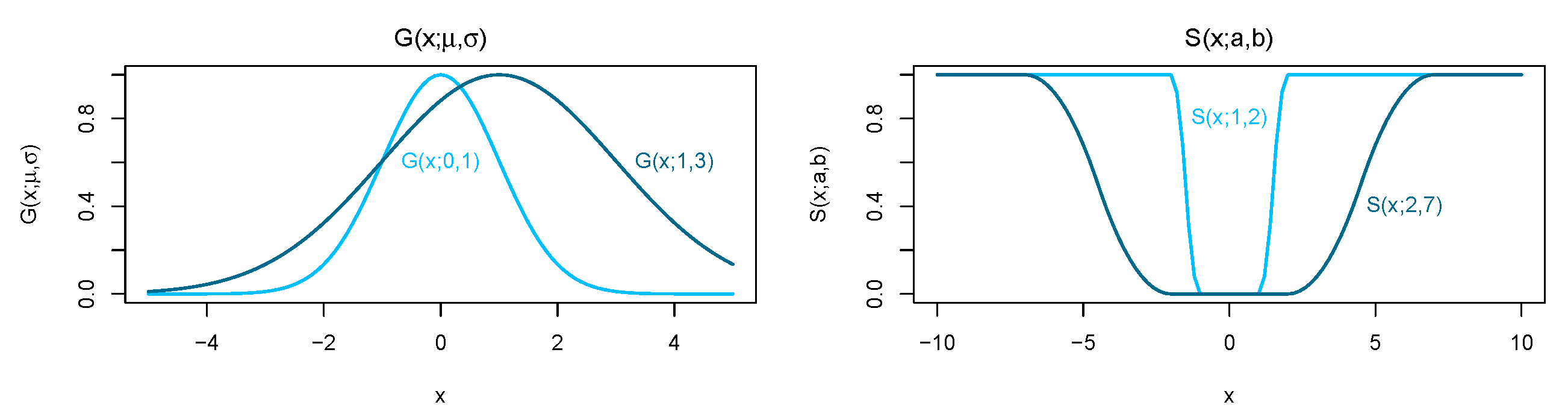
Figure 2.
Three main parts of the air traffic optimization environment’s simulation-based optimization tool TOMATO.
Figure 2.
Three main parts of the air traffic optimization environment’s simulation-based optimization tool TOMATO.
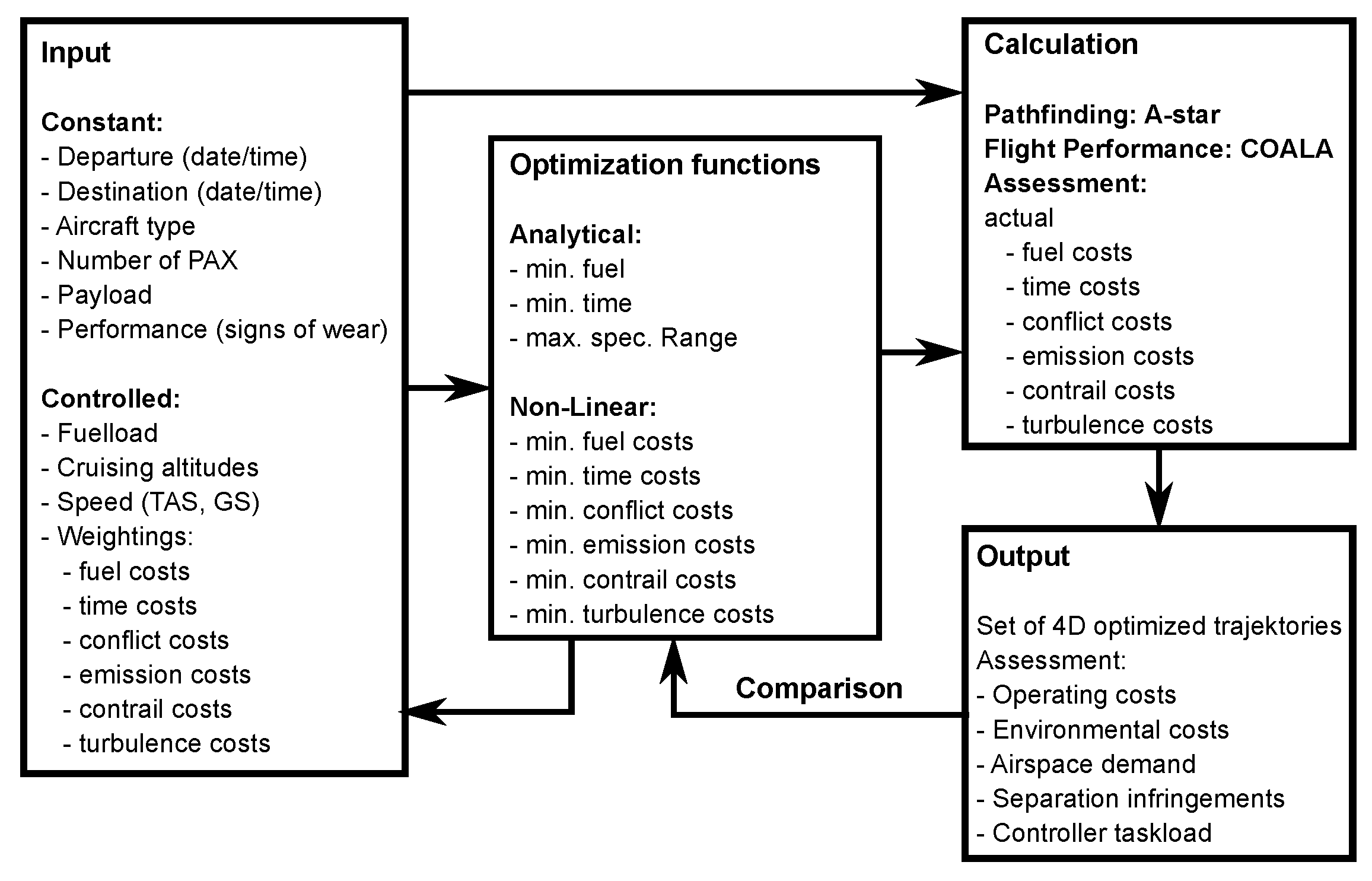
Figure 3.
SOPHIA’s control loop. To control true airspeed , the lift coefficient is employed as a regulative variable. The parameters , , , and the reset time are affected by aircraft type and mass and flight phase.
Figure 3.
SOPHIA’s control loop. To control true airspeed , the lift coefficient is employed as a regulative variable. The parameters , , , and the reset time are affected by aircraft type and mass and flight phase.
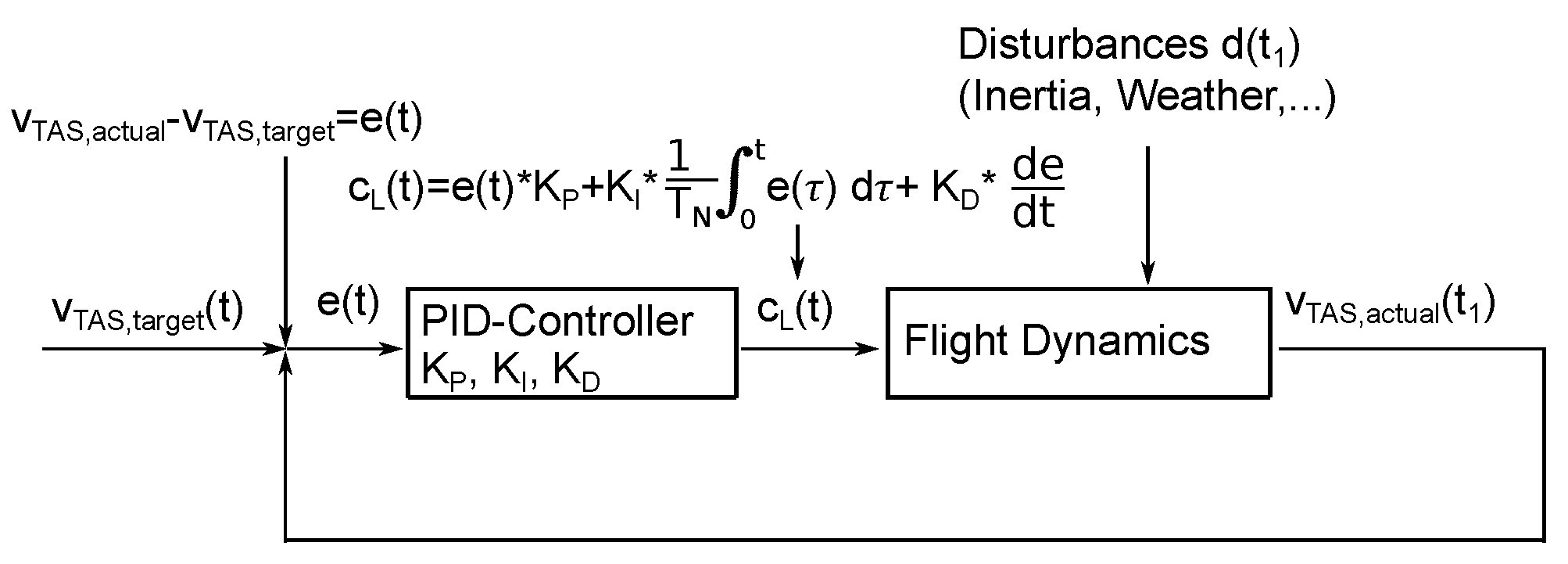
Figure 4.
Profiles of flight CSN6273 from Harbin Taiping International Airport (ZYHB) to Shenzhen Bao’an International Airport (ZGSZ). Left: The real flight (Scenario 1) has been operated below an optimum cruising altitude with numerous level flights. Optimized profiles result in similar cruising altitudes. Right: Weather-optimized profile (Scenario 3) with highlighted contrail formation (red line) and ice-supersaturated regions (blue circles). Three contrails with a total formation time of 55 min cause 592 € in environmental costs.

Figure 5.
Lateral paths of flight CSN6273 from ZYHN to ZGSZ. Left: yellow-red colour scheme indicates wind speed in knots. Middle and right: blue areas indicate ice-supersaturated regions. The real path (Scenario 1, rose) makes a detour of 7% and a contrail is induced during another 30 min of flight time (85 min, compared to 55 min in the path-optimized scenario).

Figure 6.
Profiles of flight UAL940 from Newark (KEWR) to London (EGLL). The real flight (Scenario) begins its cruise at FL350 and climbs later to FL370 and contains two level-flight segments, resulting in kg fuel burn, compared to kg for the aerodynamically optimized trajectory (Scenario 2) and kg for the weather-optimized solution (Scenario 3).
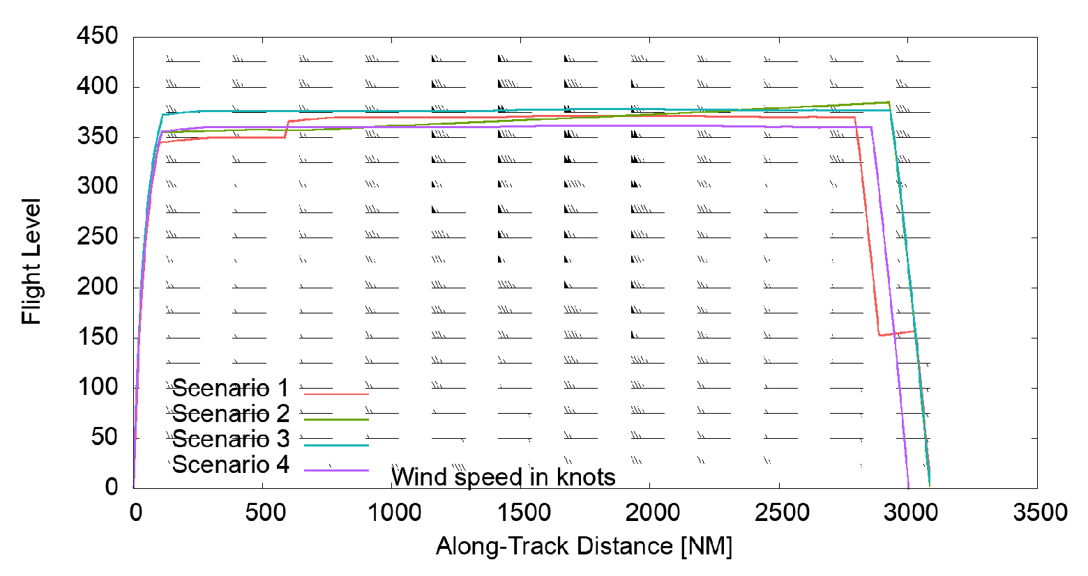
Figure 7.
Profiles of flight UAL940 from Newark (KEWR) to London (EGLL) in ice-supersaturated regions (blue circles) indicating contrail formation (red flight segments) with additional environmental costs. (Left): The real flight (rose) induced three short contrails during 55 min flight time inducing 445 € contrail costs. (Right) The multi-criteria optimized path and profile (purple) induced two long contrails during 85 min resulting in 675 € contrail costs.

Figure 8.
Lateral paths of flight UAL940 from Newark (KEWR) to London (EGLL). Yellow-red colour scheme indicates wind speed in knots. The historical flight was filed more southerly with a diversion of 150 km, which corresponds to a detour factor of %.
Figure 8.
Lateral paths of flight UAL940 from Newark (KEWR) to London (EGLL). Yellow-red colour scheme indicates wind speed in knots. The historical flight was filed more southerly with a diversion of 150 km, which corresponds to a detour factor of %.

Figure 9.
Lateral paths of flight UAL940 from Newark (KEWR) to London (EGLL). Blue areas indicate ice-supersaturated regions with contrail formation. Due to its lower cruising altitude (FL350-FL370, top), the real flight (Scenario 1, rose) produces considerably shorter contrails than the multi-criteria optimized flight at FL390 (bottom, purple). However, Scenario 1 flies a detour of %.
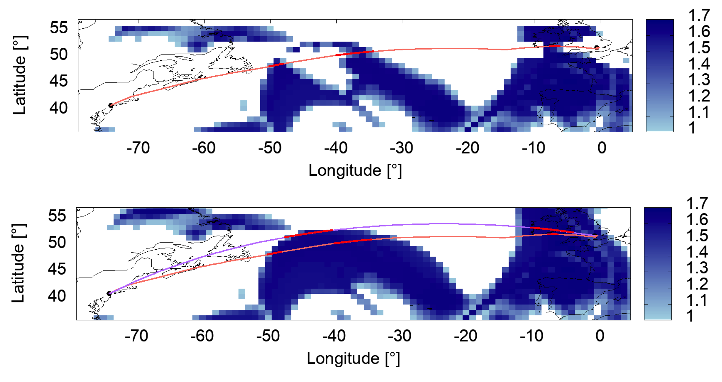
Figure 10.
Comparison of binned mean cruising altitudes per flight between aerodynamic optimized cruising altitudes (Scenario 2, left) and weather-optimized Scenario 3 (right). In most cases, Scenario 3 resulted in a minimal fuel flow. See Table 1 for scenario definition.
Figure 10.
Comparison of binned mean cruising altitudes per flight between aerodynamic optimized cruising altitudes (Scenario 2, left) and weather-optimized Scenario 3 (right). In most cases, Scenario 3 resulted in a minimal fuel flow. See Table 1 for scenario definition.

Figure 11.
(Left) Binned distances of historic flights (Scenario 1), calculated along flown lateral flight paths in China (red) and Europe (blue). Both data sets represent typical mid-haul distances between 800 NM and 1700 NM. (Right) mean cruising altitudes of historic flights (Scenario 1) in China are remarkably lower with a larger standard deviation, than in Europe.

Figure 12.
(Left) comparison of historic fuel burn with minimal fuel burn from Scenario 1:3 per flight. (Right) comparison of historic fuel burn with minimal fuel burn from Scenario 4 per flight. Red and blue lines: regression line for fuel burn values. Note, the flatter the slope of the regression lines, the greater the difference between historical and optimized fuel consumption.

Figure 13.
Histogram of VFE (Equation (1)) between historic and minimum-fuel flights (Scenario 2 or 3) in China and Europe. Here, a constant lateral flight path is used.
Figure 13.
Histogram of VFE (Equation (1)) between historic and minimum-fuel flights (Scenario 2 or 3) in China and Europe. Here, a constant lateral flight path is used.

Figure 14.
FE (Equation (13)) between historic and 3-D optimized flights in China (red) and Europe (blue).
Figure 14.
FE (Equation (13)) between historic and 3-D optimized flights in China (red) and Europe (blue).


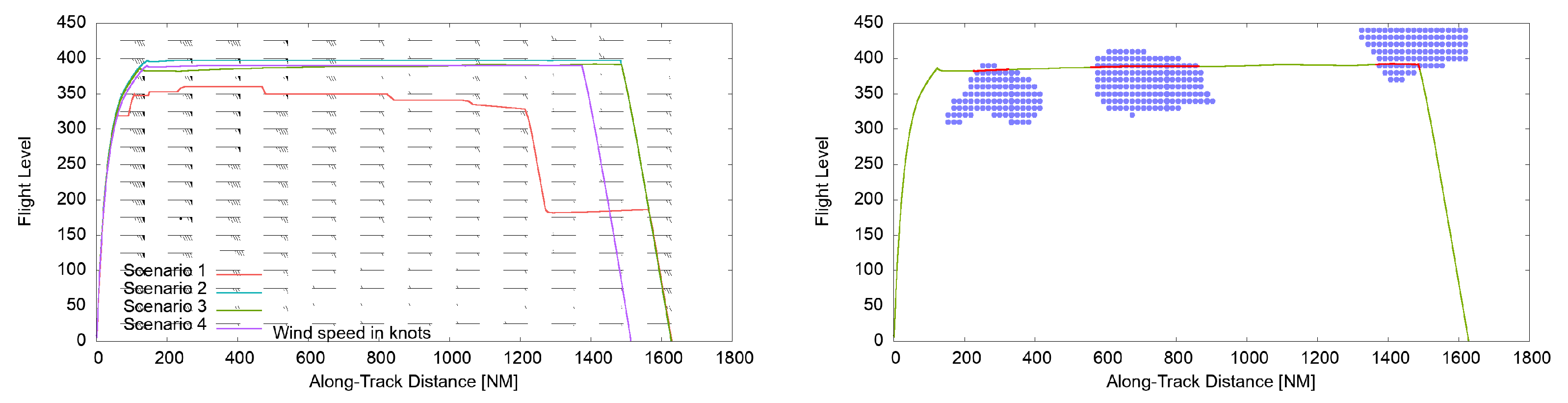
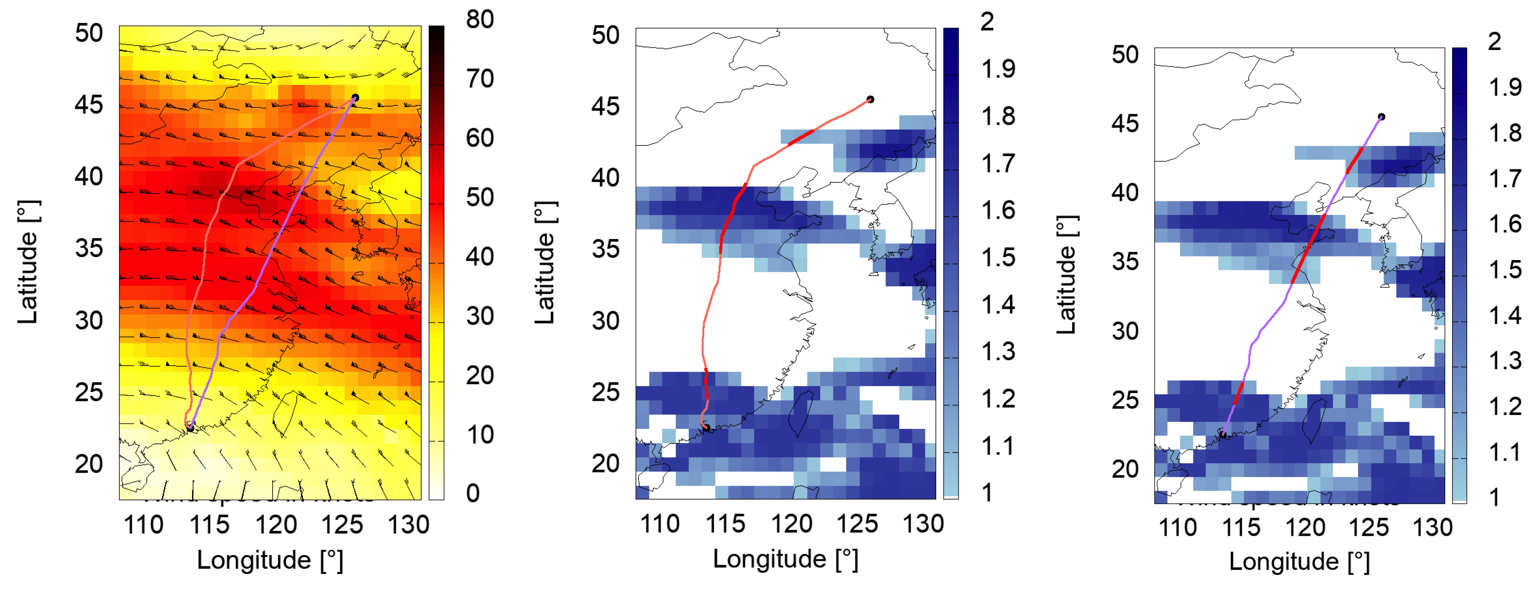
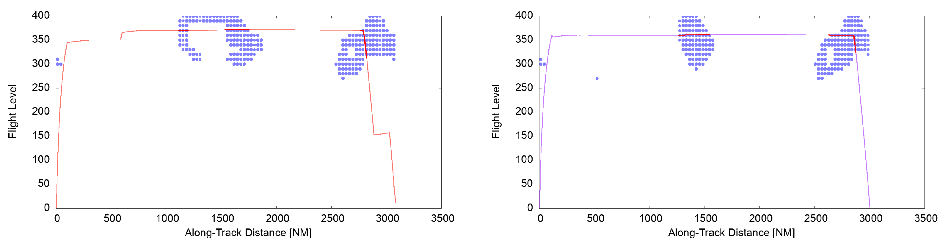
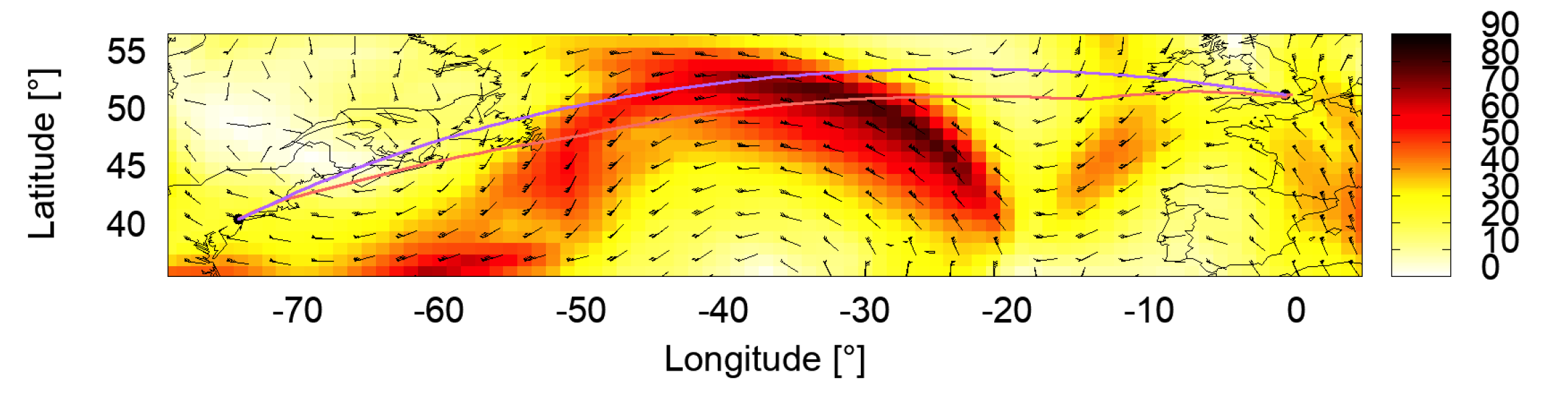
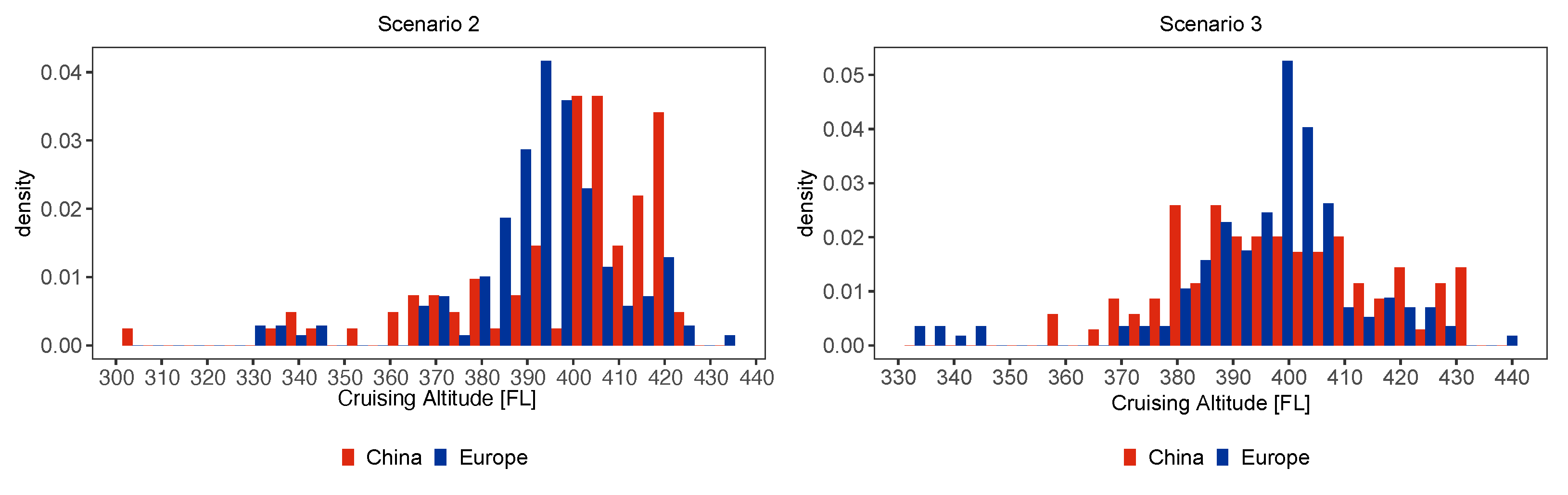
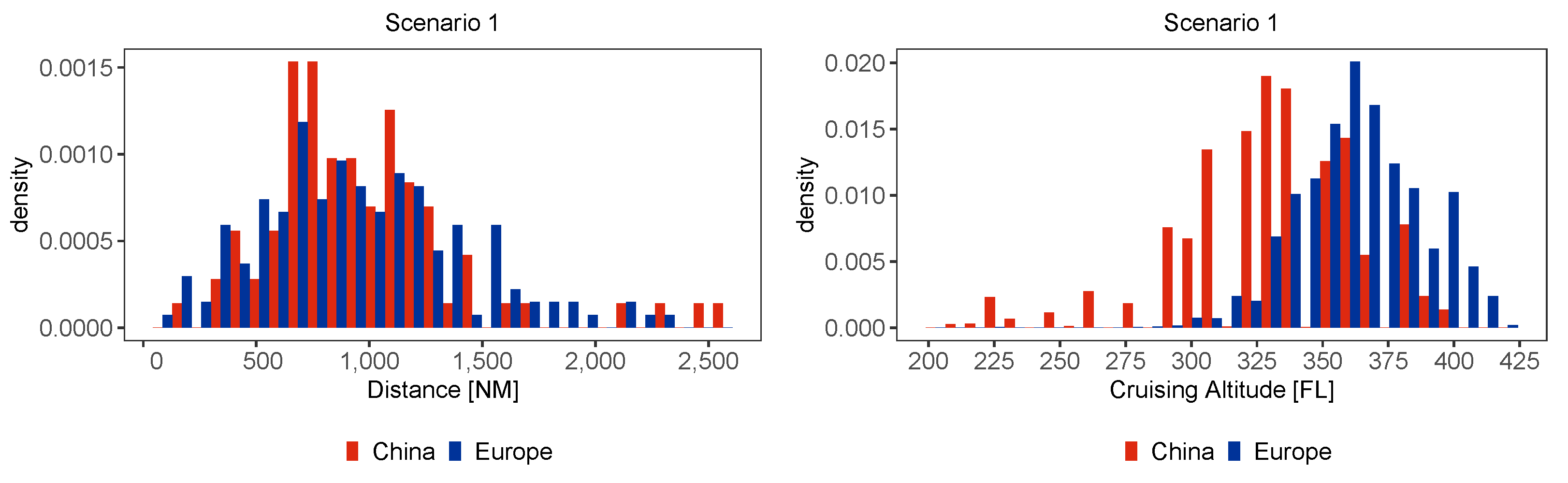
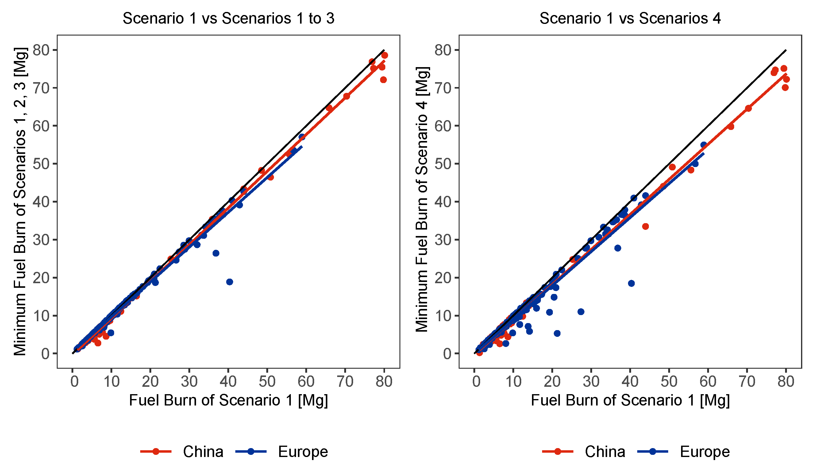
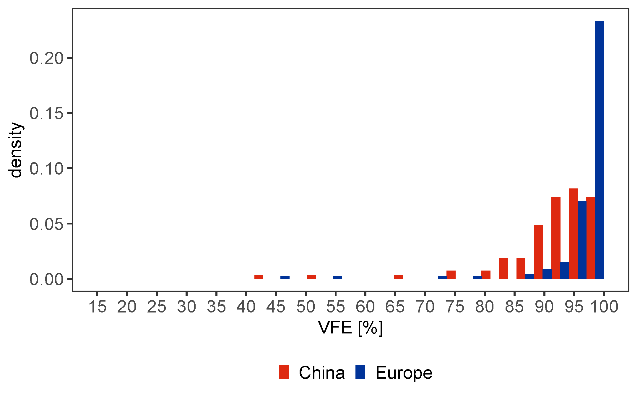
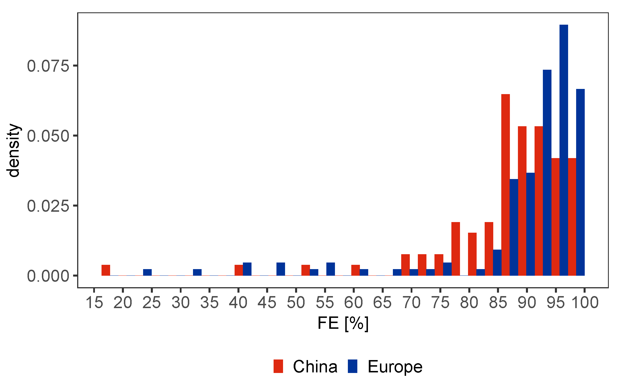
Table 1.
Four Scenarios are analyzed in this study to compare historic flights (Scenario 1) with minimum-fuel-optimized trajectories.
Table 1.
Four Scenarios are analyzed in this study to compare historic flights (Scenario 1) with minimum-fuel-optimized trajectories.
| Scenario | Optimization Target |
|---|---|
| Scenario 1 | historic vertical and lateral profile |
| Scenario 2 | aerodynamically optimized vertical profile (see Section 3.4) and historic lateral profile |
| Scenario 3 | weather-optimized vertical profile (see Section 3.5) and historic lateral profile |
| Scenario 4 | both weather-optimized vertical profile and lateral profile (see Section 3.6) |
Table 2.
Kernel function for all the phases with altitude z [ft], ground speed [kt], and Rate of Climb (RoC) [ft min] as input [40].
Table 2.
Kernel function for all the phases with altitude z [ft], ground speed [kt], and Rate of Climb (RoC) [ft min] as input [40].
| Kernel | Altitude z [ft] | Ground Speed [kt] | Rate of Climb RoC [ft min] |
|---|---|---|---|
| Ground | |||
| Climb/Descent | |||
| Cruise | |||
| Level flight |
Table 3.
Kernel function values for the data point .
| Kernel | ||||
|---|---|---|---|---|
| Ground | 1 | 0 | 1 | 0 |
| Climb/Descent | 0.06 | 0.01 | 1 | 0.01 |
| Cruise | 1 | 1 | 1 | 1 |
| Level flight | 0.06 | 0.01 | 1 | 0.01 |
Table 4.
Similarity among characteristics of the areas of investigation.
| China | Europe | |
|---|---|---|
| Coordinates: longitude [°] | [101–125] | [–25] |
| Coordinates: latitude [°] | [20–41] | [35–55] |
| Area size [km] | ||
| Inhabitants | ||
| Mean # of movements per year | ||
| Total # of trajectories | 12,721 | 18,264 |
| # of analyzed trajectories | 99 | 160 |
Table 5.
Assessment of two single trajectories with different optimization strategies. The term EPI summarizes environmental costs including contrail costs and is described in [53].
Table 5.
Assessment of two single trajectories with different optimization strategies. The term EPI summarizes environmental costs including contrail costs and is described in [53].
| Fuel | Flight | Ground | Air | Total | Contrail | Contrail | EPI | ATC | VFE | |
|---|---|---|---|---|---|---|---|---|---|---|
| Flight/Scenario | Burn | Time | Distance | Distance | Costs | Time | Costs | Charges | ||
| [kg] | [h] | [km] | [km] | [€] | [min] | [€] | [€] | [€] | [%] | |
| CSN6273 | ||||||||||
| 1 | 9595 | 4.70 | 3013 | 3299 | 35,306 | 85 | 914 | 1674 | 3933 | 90.34 |
| 2 | 8777 | 4.33 | 3013 | 3258 | 32,435 | 74 | 826 | 1528 | 3930 | 98.75 |
| 3 | 8668 | 4.31 | 3013 | 3246 | 32,092 | 55 | 592 | 1285 | 3929 | 100 |
| 4 | 8080 | 3.96 | 2966 | 2966 | 30,039 | 77 | 822 | 1469 | 3673 | - |
| UAL940 | ||||||||||
| 1 | 28,542 | 6.72 | 5711 | 5225 | 100,552 | 41 | 445 | 2950 | 6698 | 95.01 |
| 2 | 27,728 | 6.56 | 5711 | 5213 | 99,779 | 56 | 600 | 3068 | 6698 | 97.80 |
| 3 | 27,118 | 6.61 | 5711 | 5210 | 99,028 | 55 | 588 | 2896 | 6698 | 100 |
| 4 | 26,968 | 6.52 | 5561 | 5161 | 97,750 | 63 | 675 | 3115 | 6212 | - |
Table 6.
Number, distance and duration spend in level flight during climb and descent. (Note: flights with 0 level segments are excluded).
Table 6.
Number, distance and duration spend in level flight during climb and descent. (Note: flights with 0 level segments are excluded).
| # of Flights with | ||||||||||
|---|---|---|---|---|---|---|---|---|---|---|
| # of level segments | 0 | 1 | 2 | 3 | 4 | 5 | 6 | 7 | 8 | 12 |
| China | 19 | 27 | 11 | 9 | 8 | 6 | 11 | 2 | 3 | 1 |
| Europe | 81 | 66 | 6 | 1 | 2 | 3 | 1 | 0 | 0 | 0 |
| Distance flown in level [NM] | 0–50 | 50–100 | 100–150 | 150–200 | 200–250 | 250–300 | 300–350 | |||
| China | 235 | 16 | 1 | 2 | 0 | 0 | 0 | |||
| Europe | 81 | 18 | 8 | 0 | 2 | 0 | 1 | |||
| Time spent in level [min] | 0–10 | 10–20 | 20–30 | 30–40 | 40–50 | 50–60 | 60–70 | |||
| China | 244 | 7 | 3 0 | 0 | 0 | 0 | ||||
| Europe | 76 | 21 | 9 | 2 | 1 | 1 |
Table 7.
Counts and frequencies of mean cruising altitudes of historic flights (Scenario 1) and optimized flights (Scenarios 2 and 3) in China and Europe. Note: altitude 200 means the altitude bin .
Table 7.
Counts and frequencies of mean cruising altitudes of historic flights (Scenario 1) and optimized flights (Scenarios 2 and 3) in China and Europe. Note: altitude 200 means the altitude bin .
| Altitude Bin [FL] | 200 | 220 | 240 | 260 | 280 | 300 | 320 | 340 | 360 | 380 | 400 | 420 | 440 |
|---|---|---|---|---|---|---|---|---|---|---|---|---|---|
| Scenario 1: China | |||||||||||||
| # of flights | 1 | 4 | 5 | 4 | 11 | 19 | 25 | 13 | 7 | 0 | 0 | 0 | 0 |
| frequency | 0.001 | 0.002 | 0.003 | 0.002 | 0.006 | 0.011 | 0.014 | 0.007 | 0.004 | 0 | 0 | 0 | 0 |
| Scenario 1: Europe | |||||||||||||
| # of flights | 0 | 0 | 0 | 0 | 2 | 4 | 19 | 50 | 50 | 25 | 6 | 0 | 0 |
| frequency | 0 | 0 | 0 | 0 | 0.001 | 0.001 | 0.006 | 0.016 | 0.016 | 0.008 | 0.002 | 0 | 0 |
| Scenario 2: China | |||||||||||||
| # of flights | 0 | 0 | 0 | 0 | 0 | 1 | 3 | 2 | 11 | 14 | 51 | 10 | 0 |
| frequency | 0 | 0 | 0 | 0 | 0 | 0.001 | 0.002 | 0.001 | 0.006 | 0.008 | 0.028 | 0.005 | 0 |
| Scenario 2: Europe | |||||||||||||
| # of flights | 0 | 0 | 0 | 0 | 0 | 0 | 5 | 2 | 16 | 89 | 36 | 7 | 0 |
| frequency | 0 | 0 | 0 | 0 | 0 | 0 | 0.002 | 0.001 | 0.005 | 0.029 | 0.012 | 0.002 | 0 |
| Scenario 3: China | |||||||||||||
| # of flights | 0 | 0 | 0 | 0 | 0 | 0 | 0 | 2 | 11 | 40 | 27 | 15 | 0 |
| frequency | 0 | 0 | 0 | 0 | 0 | 0 | 0 | 0.001 | 0.006 | 0.021 | 0.014 | 0.008 | 0 |
| Scenario 3: Europe | |||||||||||||
| # of flights | 0 | 0 | 0 | 0 | 0 | 0 | 5 | 2 | 11 | 72 | 55 | 10 | 0 |
| frequency | 0 | 0 | 0 | 0 | 0 | 0 | 0.002 | 0.001 | 0.004 | 0.023 | 0.018 | 0.003 | 0 |
Table 8.
The number of minimum-fuel flights for each scenario in China (92 flights in total) and Europe (159 flights in total). See Table 1 for scenario definition.
Table 8.
The number of minimum-fuel flights for each scenario in China (92 flights in total) and Europe (159 flights in total). See Table 1 for scenario definition.
| Scenario 1 | Scenario 2 | Scenario 3 | Scenario 4 | |
|---|---|---|---|---|
| China | 0 | 2 | 11 | 79 |
| Europe | 0 | 4 | 12 | 143 |
Table 9.
Mean, median, and standard deviation (sd) of VFE (Equation (1)) between historic and minimum-fuel flights (Scenario 2 or 3) in China and Europe, considering a constant lateral flight path in each scenario.
Table 9.
Mean, median, and standard deviation (sd) of VFE (Equation (1)) between historic and minimum-fuel flights (Scenario 2 or 3) in China and Europe, considering a constant lateral flight path in each scenario.
| VFE [%] | China | Europe |
|---|---|---|
| mean | 91.62 | 96.61 |
| median | 93.69 | 98.32 |
| sd | 8.87 | 6.37 |
Table 10.
Mean, median, and standard deviation of FE (Equation (13)) between historic and 3-D optimized flights in China and Europe.
Table 10.
Mean, median, and standard deviation of FE (Equation (13)) between historic and 3-D optimized flights in China and Europe.
| FE [%] | China | Europe |
|---|---|---|
| mean | 87.32 | 89.84 |
| median | 89.33 | 93.84 |
| sd | 12.64 | 13.20 |
Publisher’s Note: MDPI stays neutral with regard to jurisdictional claims in published maps and institutional affiliations. |
© 2022 by the authors. Licensee MDPI, Basel, Switzerland. This article is an open access article distributed under the terms and conditions of the Creative Commons Attribution (CC BY) license (https://creativecommons.org/licenses/by/4.0/).
Share and Cite
MDPI and ACS Style
Rosenow, J.; Chen, G.; Fricke, H.; Wang, Y. Factors Impacting Chinese and European Vertical Fight Efficiency. Aerospace 2022, 9, 76. https://doi.org/10.3390/aerospace9020076
AMA Style
Rosenow J, Chen G, Fricke H, Wang Y. Factors Impacting Chinese and European Vertical Fight Efficiency. Aerospace. 2022; 9(2):76. https://doi.org/10.3390/aerospace9020076
Chicago/Turabian StyleRosenow, Judith, Gong Chen, Hartmut Fricke, and Yanjun Wang. 2022. "Factors Impacting Chinese and European Vertical Fight Efficiency" Aerospace 9, no. 2: 76. https://doi.org/10.3390/aerospace9020076
Note that from the first issue of 2016, this journal uses article numbers instead of page numbers. See further details here.