A Pixel-Wise Foreign Object Debris Detection Method Based on Multi-Scale Feature Inpainting

Abstract

In the aviation industry, foreign object debris (FOD) on airport runways is a serious threat to aircraft during takeoff and landing. Therefore, FOD detection is important for improving the safety of aircraft flight. In this paper, an unsupervised anomaly detection method called Multi-Scale Feature Inpainting (MSFI) is proposed to perform FOD detection in images, in which FOD is defined as an anomaly. This method adopts a pre-trained deep convolutional neural network (CNN) to generate multi-scale features for the input images. Based on the multi-scale features, a deep feature inpainting module is designed and trained to learn how to reconstruct the missing region masked by the multi-scale grid masks. During the inference stage, an anomaly map for the test image is obtained by computing the difference between the original feature and its reconstruction. Based on the anomaly map, the abnormal regions are identified and located. The performance of the proposed method is demonstrated on a newly collected FOD dataset and the public benchmark dataset MVTec AD. The results show that the proposed method is superior to other methods.

1. Introduction

In the field of aviation, foreign object debris (FOD) refers to objects that appear on the pavements of the whole movement area, including an airport’s runways, taxiways and apron and may cause damage to the aircraft, such as screws, nuts, rubber blocks, stones, etc. [1]. Since the presence of FOD may pose a huge potential risk to aircraft during takeoff and landing, it needs to be removed from the runway in time. Therefore, FOD detection is an indispensable part of airport operation. Traditional FOD detection and removal methods, which rely on the staff to check runways and other regions at regular intervals, are inefficient. In addition, the reliability of traditional methods is also unsatisfactory. Small-scale FODs, such as nuts similar in color to airport runways, are not easily detected by the naked eye. Visual inspection systems are now widely adopted for automatic FOD detection. Meanwhile, FOD detection has become a hot spot in academic research, and many achievements have been attained [2,3,4,5].

Deep-learning-based methods are widely used in object detection due to their effectiveness and universality [6,7,8,9]. However, the lack of labeled FOD images remains a major challenge in FOD detection tasks. In general, deep-learning-based detection methods require massive labeled images and a long period of supervised training. However, a comprehensive and balanced dataset, including different FOD, is very difficult to collect and annotate in actual airport environments, making the model lack effectively supervised information. More importantly, because FOD could be anything accidentally dropped on airport runways, the model trained using only limited FOD samples may fail to generalize on those previously unseen ones. Therefore, the supervised learning-based methods are not the best choice for FOD detection. Conversely, the unsupervised anomaly detection method is expected to solve this problem. In the basic anomaly detection tasks, only normal samples are available for training to construct a machine learning system that can detect abnormal samples [10,11], which is exactly the goal of FOD detection tasks. In FOD detection tasks, although images with real FOD are rare, images without FOD are sufficient for training. Since labeled FOD samples are not required, unsupervised anomaly detection methods can quickly adapt to different airport environments.

Recently anomaly detection methods for image focus on reconstructing the original image to a normal image through an autoencoder network [12,13,14]. The input image is assigned an anomaly score based on the reconstruction error. This method assumes that the model trained on normal images cannot be generalized to abnormal images, that is, the reconstruction error of abnormal images is higher than that of normal images. However, this assumption is not always true in practice because the model has strong generalization ability and may reconstruct abnormal images well, which makes abnormal regions indistinguishable from normal regions only by the reconstruction error.

The methods based on pre-trained deep convolutional neural networks (CNNs) have recently been proposed for image anomaly detection [15,16,17]. The pre-trained CNNs are very helpful when the dataset is small and the normal regions show randomness. They try to model the distribution of the pre-trained features of normal data using Gaussian mixture models or clustering. In the inference process, if the pre-trained features of the image deviate from the distribution, it is identified as an anomaly. These methods provide excellent results on image-level anomaly detection. However, they cannot perform anomaly localization. To tackle this problem, many methods perform in a region-based fashion, which splits images into smaller patches and determines the abnormality of every patch. This demands high computational resources and often leads to inaccurate localization.

In this work, we also leverage the pre-trained CNNs to detect anomalies. However, we propose to train a feature inpainting model in a self-supervised manner to restore the damaged feature maps into normal ones instead of modeling the distribution of the pre-trained features. The trained model can thus detect abnormal regions by comparing the original and restored features of the image. In particular, multi-scale grid masks are designed to determine the removal and recovery regions in the feature maps. The proposed method is termed as multi-scale feature inpainting (MSFI), where it realizes unsupervised anomaly detection and localization by reconstructing incomplete multi-scale features generated from the pre-trained CNN. Extensive experiments on two datasets, MVTec AD [18] and FOD, are conducted for image-level anomaly detection and pixel-level anomaly localization.

The rest of this paper is organized as follows. Section 2 discusses the latest methods of image anomaly detection. Section 3 introduces the overall anomaly detection framework in detail. In Section 4 and Section 5, the experimental conditions are introduced and the experimental results are shown, respectively. Section 6 presents the ablation study. Section 7 and Section 8 provide the discussion and conclusion of this paper, respectively.

2. Related Work

Unsupervised image anomaly detection methods require only normal images during training. These methods can be divided into two methods: image reconstruction and feature modeling.

In many recent image reconstruction-based anomaly detection methods, autoencoders and a range of variants have been widely used, such as autoencoders [19,20] and variational autoencoders [21,22]. The core idea of these methods is to convert an image into an abstract representation and then try to find its inverse mapping to reconstruct the original image. They assumed that the model trained on normal samples could not reproduce abnormal samples. However, the autoencoder could not only generalize well but could reconstruct the abnormal samples well [23,24]. To address this problem, Gong et al. [24] proposed the memory-augmented autoencoder that designs a memory module for recording representations of normal samples. As the reconstruction consists of representations of normal samples, the reconstruction errors of abnormal samples will be increased. Generative adversarial network (GAN) [25] is also a network used for reconstruction, which aims to improve the quality of reconstruction through adversarial training. For example, Schlegl et al. [26] took the lead in using generative adversarial networks (GAN) for image anomaly detection and proposed AnoGAN. In addition, some methods [27,28] perform anomaly detection by masking multiple regions of the input image and using an autoencoder to reconstruct the masked regions only from its neighborhood information rather than the information of the region being reconstructed. It is assumed that the possibility of accurately reconstructing abnormal regions by generalizing neighborhood appearances is very low. For instance, Li et al. [27] proposed superpixel masking and inpainting (SMAI), which combines superpixel segmentation to determine the missing regions of an image.

Unlike the model based on image reconstruction, which detects anomalies in the image space, feature-modeling-based methods [29,30,31,32] detect anomalies in the feature space. For example, Ruff et al. [33] proposed deep support vector data description (Deep SVDD), which trains a neural network while minimizing the volume of the hypersphere containing normal sample representation. Since the network must map normal samples closely to the hypersphere’s center, minimizing the hypersphere’s volume forces the network to extract common features of the normal samples. However, since Deep SVDD maps the whole image to a point in the feature space, it can only infer whether there is an anomaly in the image and cannot indicate the location of the abnormal regions. Therefore, Patch SVDD was proposed, which detects each patch to localize anomalies [34]. More recently, Bergmann et al. [35] proposed a student–teacher knowledge distillation framework for unsupervised anomaly detection, which uses the deep features from the pre-trained CNNs to detect anomalies in images through feature regression. Specifically, a pre-trained CNN (e.g., resnet18 [36]) is defined as a teacher network and several simple networks are defined as the student networks. During the training, the student networks are trained to imitate the behavior of the teacher network only on normal images. During the test, the anomaly score is calculated based on the predicted errors between the output of the teacher network and the student networks. The method assumes that the student networks only learn how to regress the output of the teacher network on normal images. Thus, the student networks may not be able to predict the output of the teacher network on abnormal images.

3. Method

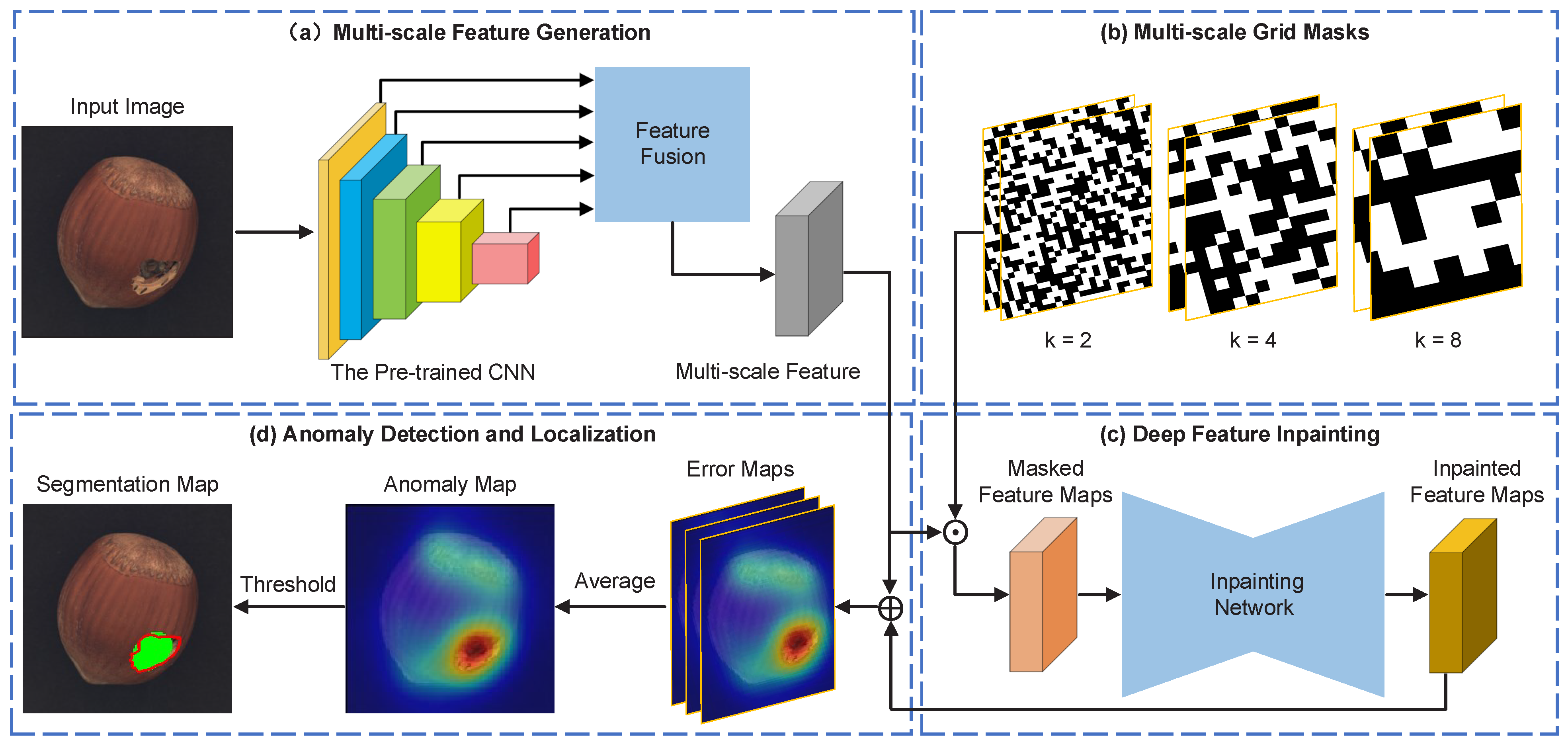
Figure 1 shows the framework of the multi-scale feature inpainting (MSFI) for image anomaly detection, which contains four parts: multi-scale feature generation module, multi-scale grid masks module, deep feature inpainting module, and anomaly detection and localization module. Given an input image, first the multi-scale features are constructed using the pre-trained CNN. Then, the multi-scale features are transformed to the masked feature maps via the multi-scale grid masks. Following this, the deep feature inpainting model recover and reconstruct each masked feature map. Finally, the anomaly map is obtained through calculation of the $l{}_2$ value of the original feature and its reconstruction version. The framework will be detailed in the following sections.

3.1. Multi-Scale Feature Extraction

A pre-trained CNN is used to generate discriminative deep features, which are then fed into the deep feature inpainting module with the multi-scale grid mask.

It is supposed that there is a CNN with L convolutional blocks, and each convolutional block consists of multiple consecutive convolutional layers and pooling layers. I represents an input image with the size of $h\times w\times c$. Feeding I into the CNN, a set of feature maps $\left\{{\varphi }_1\left(I\right),{\varphi }_2\left(I\right),\dots ,{\varphi }_L\left(I\right)\right\}$ from the L convolutional blocks can be obtained. The size of the l-th feature map ${\varphi }_l\left(I\right)$ is $h_l\times w_l\times c_l$. Since each feature map comes from a convolutional layer with a specific receptive field, it represents an abstract representation of the input image. In general, the low convolutional layers with small receptive field capture low-level features or local structural information, such as textural structure. In contrast, the deep convolutional layers with a large receptive field capture high-level features or global semantic information. Therefore, the fusion of the feature maps ${\left\{{\varphi }_l\left(I\right)\right\}}_{l=1}^L$ naturally forms a discriminative representation for the image. The process of fusion consists of two steps, as shown in Equation (1). First, the feature map ${\varphi }_l\left(I\right)$ is resized to the space size $\left(h_0,w_0,c_l\right)$, but the channel is unchanged. Then, all the scaled feature maps are concatenated to an integrated feature map:

$$f\left(I\right)=cat\left(resize\left({\varphi }_1\left(I\right),{\varphi }_2\left(I\right),\dots ,{\varphi }_L\left(I\right)\right)\right)$$

(1)

where $resize\left(·\right)$ denotes the function of resizing. $cat\left(·\right)$ denotes the function of concatenating. $f\left(I\right)$ denotes the generated multi-scale feature with the size of $\left(h_0,w_0,c_0\right)$. $c_0$ is the number of channels and satisfies $c_0={\sum }_{l=1}^L{c}_l$.

3.2. Multi-Scale Grid Masks

As mentioned above, MSFI first removes a part of the regions in the multi-scale feature map and then makes the deep feature inpainting network learn to generate the original feature map. One problem during the process is which part of the regions should be removed. To solve this issue, two design principles are presented. On the one hand, since the anomalies may appear anywhere in the feature map, the regions should have equal probability to be removed. On the other hand, since the anomalies may have different sizes, the removed regions should have multiple scales.

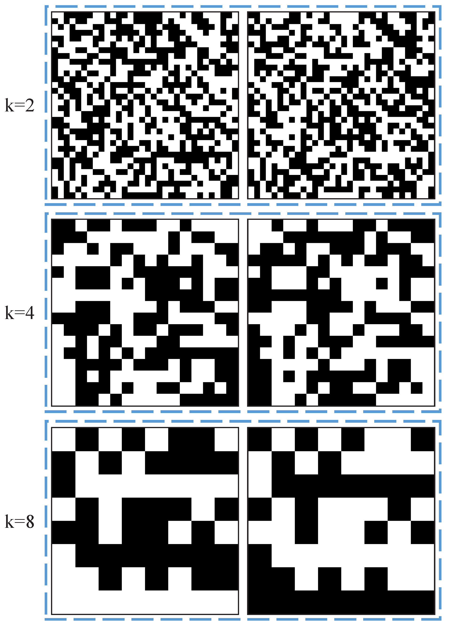
To meet these requirements, multi-scale grid masks are designed to indicate the regions that should be removed and the pixel values at the removed regions are set as zero. As shown in Figure 2, the black grids indicate the regions to be removed, and the number of white girds is equal to that of black grids. The multi-scale grid masks are generated as follows. A mask with the same size as the input feature map is first divided into $\frac{h_0}{k}\times \frac{w_0}{k}$ grids, where k is the size of the grid. Then, all grids are randomly divided into two disjoint sets $S_g$, each containing half of the grids, where $g\in \left\{1,2\right\}$. Following this, a mask $M_{S_g}$ is generated for each grid set $S_g$. $M_{S_g}$ is a binary mask in which the pixel values at the regions belonging to $S_g$ are set as zero. The masks with different scales could be obtained by changing the grid size. In this paper, three grid sizes are adopted, namely, $K=\left\{2,4,8\right\}$.

3.3. Deep Feature Inpainting

The U-Net network [37] is adopted to recover the removed regions in the multi-scale feature map. During the training, a pair of binary masks $M_{S_g}$ are first generated using a grid size k, which is randomly selected from set $K=\left\{2,4,8\right\}$ and leveraged to set the regions belong to $S_g$ as zero in the multi-scale feature map $f\left(I\right)$:

$$f_{S_g}\left(I\right)=M_{S_g}\odot f\left(I\right),g=1,2$$

(2)

where $f_{S_g}\left(I\right)$ is the masked feature map; ⊙ means the element-wise multiplication.

Then, the masked feature maps $f_{S_g}\left(I\right)$ are fed into the network sequentially. The network reconstructs each masked feature map individually and outputs the partially reconstructed feature map $f_{r_g}\left(I\right)$. Finally, the partially reconstructed feature map $f_{r_g}\left(I\right)$ are masked and summed into the entire reconstructed feature map $f_r\left(I\right)$:

$$f_r\left(I\right)=\sum _{g=1}^2\left(1_{h_0\times w_0}-M_{S_g}\right)\odot f_{r_g}\left(I\right)$$

(3)

where $1_{h_0\times w_0}$ represents a matrix with the height $h_0$ and the width $w_0$, in which the elements are all one.

The entire reconstructed feature map $f_r\left(I\right)$ is constructed using the partially reconstructed feature map $f_{r_g}\left(I\right)$, in which the value of the regions not belonging to $S_g$ are zero. Therefore, each $f_{r_g}\left(I\right)$ contributes only the regions belonging to $S_g$ that are removed in the original feature map.

The network is trained with a joint loss that takes into account the distance loss $L_{val}$ and directional similarity loss $L_{dir}$. $L_{val}$ is the averaged pixel-level $l_2$ distance between the reconstructed feature $f_r\left(I\right)$ and the original feature $f\left(I\right)$, as shown in Equation (4). The smaller the distance, the higher the similarity between the two:

$$L_{val}=\frac{1}{h_0\times w_0}\sum _{i=1}^{h_0}\sum _{j=1}^{w_0}{∥f_{r,i,j}\left(I\right)-f_{i,j}\left(I\right)∥}_2$$

(4)

where $(i,j)$ is the spatial position on deep feature maps.

$L_{dir}$ aims to increase the directional similarity between feature description vectors. Cosine similarity is used to measure the directional similarity between the reconstructed feature $f_r\left(I\right)$ and the original feature $f\left(I\right)$. The greater the cosine value, the higher the directional similarity between the two. The $L_{dir}$ is defined as:

$$L_{dir}=1-\frac{vec{\left(f\left(I\right)\right)}^T·vec\left(f_r\left(I\right)\right)}{∥vec\left(f\right(I\left)\right)∥∥vec\left(f_r\left(I\right)\right)∥}$$

(5)

where $vec(·)$ is a vectorization function transforming a matrix with arbitrary dimensions into a one-dimensional vector.

Finally, the total loss function is defined as:

$$L_{total}={\lambda }_{val}{L}_{val}+{\lambda }_{dir}{L}_{dir}$$

(6)

where ${\lambda }_{val}$ and ${\lambda }_{dir}$ are the hyper-parameters to balance the weights of the distance loss and directional similarity loss.

3.4. Anomaly Detection and Localization

During testing, multiple masks with different grid sizes are adopted to remove regions from the multi-scale feature map and merge the multiple outputs from the model to compute the final anomaly map.

Given a test image I, the multi-scale feature map $f\left(I\right)$ is first extracted. Then, the deep feature map is masked and reconstructed several times for each $k\in K$. The anomaly map $A\left(I\right)$ for a grid size k is defined as the pixel-level $l_2$ distance between the original feature $f\left(I\right)$ and its reconstruction $f_r\left(I\right)$:

$$A\left(I\right)={∥f_r\left(I\right)-f\left(I\right)∥}_2$$

(7)

The final anomaly map $A_{final}\left(I\right)$ is then obtained by taking the average of the anomaly maps $A_k\left(I\right)$:

$$A_{final}\left(I\right)=\frac{1}{N}\sum _{k\in K}^{}{A}_k\left(I\right)$$

(8)

where $A_k\left(I\right)$ is the anomaly map generated using the grid size k as defined in Equation (7). N is the number of the grid size k.

Finally, the image-level anomaly score S is calculated by taking the maximum of $A_{final}\left(I\right)$:

$$S=max\left(A_{final}\left(I\right)\right)$$

(9)

The spatial size of $A_{final}\left(I\right)$ is $h_0\times w_0$. To further obtain the anomaly map with the same size as the image, $A_{final}\left(I\right)$ performs bilinear interpolation. To obtain the segmentation result, the anomaly map $A_{final}\left(I\right)$ is binarized using the threshold, which is the anomaly score corresponding to the maximum $F_1$ score on the test set.

4. Experimental Setup

4.1. Datasets

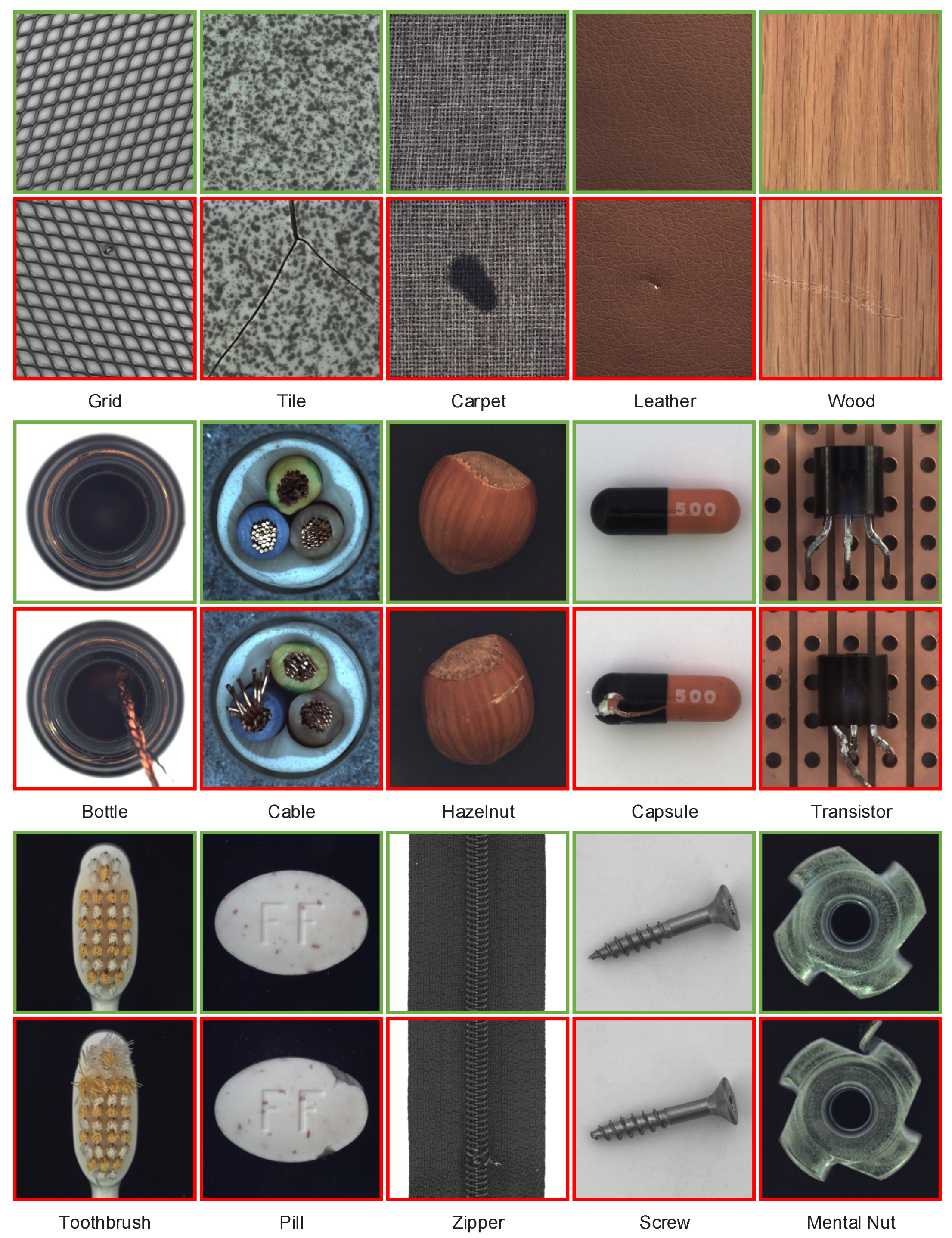
Specially designed to evaluate the performance of unsupervised image anomaly detection methods, the MVTec AD dataset has 5354 images. It contains 10 object classes and 5 texture classes with more than 70 different types of anomalies, such as breaks, contamination, holes and other structural defects. The images of each class are divided into training set and testing set, in which the former contains only normal images, while the latter contains both normal and abnormal images. Each abnormal image has a pixel-level annotation; thus, the MVTec AD dataset is well suited for evaluating unsupervised image anomaly detection methods. The Figure 3 shows many examples of normal and abnormal images in MVTec AD dataset.

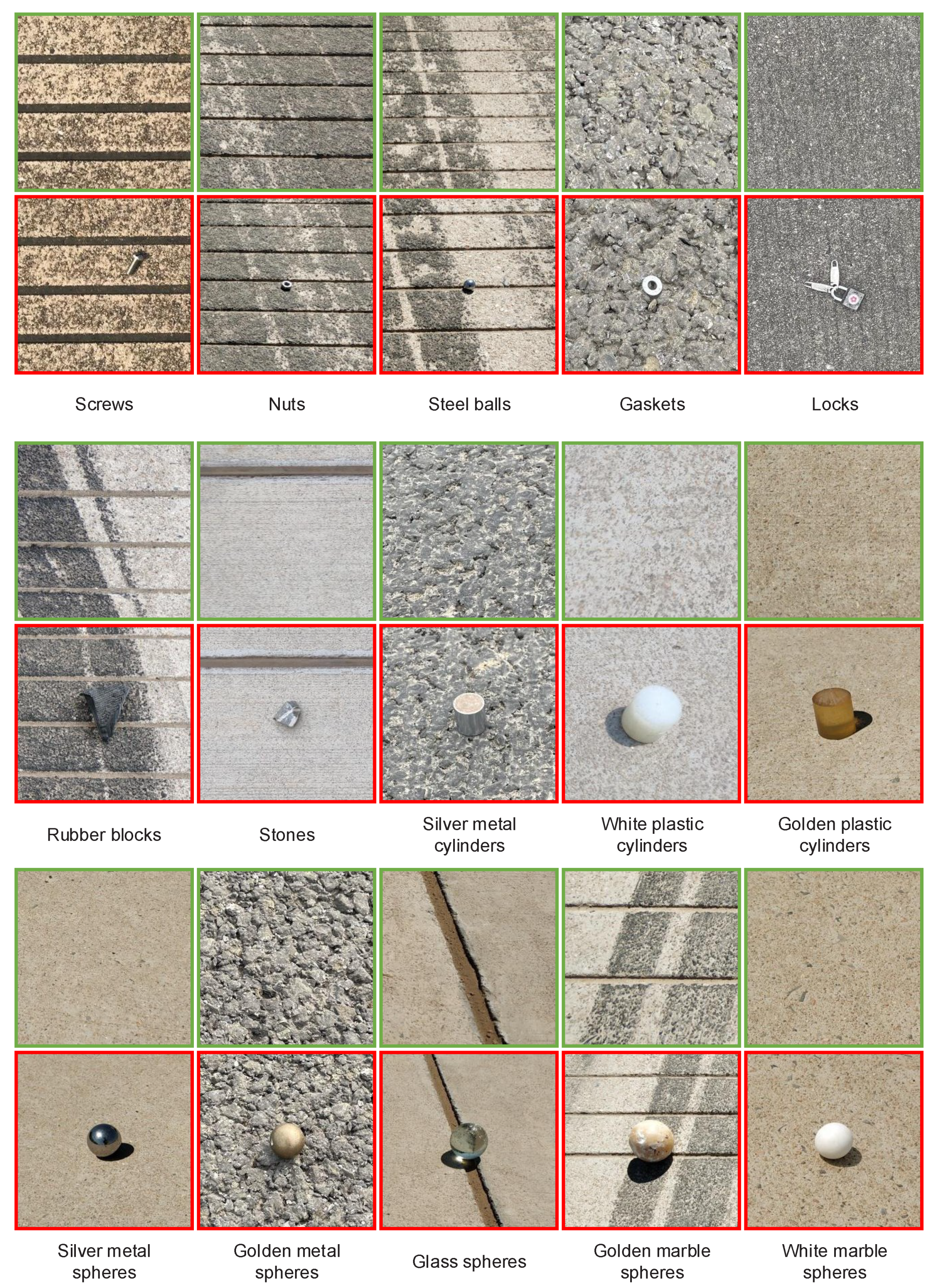
Specifically designed for FOD detection, FOD dataset is structured the same as MVTec AD dataset (i.e., the training set contains only normal images, and the testing set has both normal and abnormal images). Normal image refers to the absence of FOD on the airport runways, and an abnormal image refers to the presence of FOD on the airport runways. FOD dataset includes 9042 images. To achieve the diversity in the FOD dataset, the images containing different FOD samples and runway surface disturbances are collected. FOD samples contains 15 objects which cover different real FOD collected from the airport runways or standard samples made by factories. Real FOD samples include screws, nuts, steel balls, gaskets, locks, clamps, rubber blocks and stones, which are found most frequently on the airport runways. Standard samples contain metal cylinders, plastic cylinders, metal spheres, glass spheres and marble spheres. Runway surface disturbances include tire marks, marker lines, splice joints, holes and others. Each abnormal image provides pixel-level annotation. Examples of normal and abnormal images for the FOD dataset are shown in Figure 4.

4.2. Evaluation Metrics

The proposed method is evaluated in terms of image-level anomaly detection and pixel-level anomaly localization. The area under the receiver operating characteristic curve (AUROC) [18] is used as the evaluation metric. In addition, image-level AUROC is used to evaluate the performance for anomaly detection, while pixel-level AUROC evaluates the performance for anomaly localization. F1 score is also reported to evaluate the performance of MSFI and baselines.

4.3. Implementation Details

In the deep feature extraction module, the VGG19 [38] pre-trained on ImageNet [39] was used to produce deep features. The last three full connection layers were removed, and the output feature maps from the final four convolutional blocks were selected for feature fusion. For all the experiments on MVTec AD and FOD datasets, the deep feature inpainting network was trained by Adam optimizer with a batch size of 4 for 300 epochs. The initial learning rate was set as $1\times {10}^{-4}$. After 200 epochs, the learning rate decayed to $1\times {10}^{-5}$. During training, the weights of the pre-trained VGG19 were froze, and only the weights of the deep feature inpainting network were updated. The proposed model was implemented using the deep learning framework Pytorch.

5. Results

MSFI is evaluated on MVTec AD and FOD datasets in terms of anomaly detection and localization and is compared with the existing methods such as AE-$l_2$ [19], RIAD [40], MRKD [31] and DFR [41].

5.1. Anomaly Detection

Table 1. The anomaly detection results on MVTec AD dataset. The best result for each class is bolded.

Category	AE-${\mathit{l}}_2$		RIAD		MRKD		DFR		MSFI
	AUROC	F1	AUROC	F1	AUROC	F1	AUROC	F1	AUROC	F1
Carpet	0.539	0.863	0.842	0.859	0.792	0.859	0.961	0.938	0.976	0.960
Grid	0.779	0.855	0.996	0.957	0.780	0.862	0.968	0.927	0.921	0.922
Leather	0.841	0.865	1.000	0.956	0.950	0.847	0.984	0.963	1.000	0.995
Tile	0.795	0.847	0.987	0.850	0.915	0.830	0.896	0.883	0.870	0.894
Wood	0.892	0.902	0.930	0.884	0.942	0.923	0.981	0.977	0.996	0.983
Bottle	0.877	0.889	0.999	0.968	0.993	0.855	0.993	0.980	1.000	0.986
Cable	0.477	0.755	0.819	0.755	0.891	0.755	0.831	0.809	0.967	0.923
Capsule	0.660	0.904	0.884	0.906	0.804	0.926	0.975	0.983	0.888	0.943
Hazelnut	0.951	0.924	0.833	0.865	0.983	0.843	0.989	0.982	0.995	0.978
Metal Nut	0.415	0.889	0.885	0.893	0.735	0.889	0.929	0.921	0.955	0.963
Pill	0.625	0.912	0.838	0.919	0.827	0.912	0.931	0.928	0.942	0.954
Screw	0.746	0.878	0.845	0.865	0.833	0.863	0.958	0.931	0.866	0.878
Toothbrush	0.589	0.829	1.000	0.967	0.921	0.817	0.981	0.964	0.969	0.933
Transistor	0.703	0.619	0.909	0.619	0.855	0.569	0.801	0.787	0.964	0.916
Zipper	0.765	0.881	0.981	0.963	0.932	0.877	0.903	0.915	0.925	0.955
Mean	0.710	0.854	0.917	0.882	0.877	0.842	0.939	0.926	0.949	0.945

shows the anomaly detection results on the MVTec AD dataset. MSFI records the highest AUROC in nine categories and is superior to other anomaly detection methods in terms of average AUROC. In addition, MSFI outperforms the best baseline method DFR by 1%.

Table 2. The anomaly detection results on FOD dataset. The best result for each class is bolded.

Category	AE-${\mathit{l}}_2$		RIAD		MRKD		DFR		MSFI
	AUROC	F1	AUROC	F1	AUROC	F1	AUROC	F1	AUROC	F1
Screws	0.715	0.712	0.788	0.754	0.933	0.908	0.777	0.775	0.997	0.947
Nuts	0.670	0.629	0.759	0.758	0.944	0.897	0.975	0.970	0.995	0.954
Steel balls	0.713	0.710	0.741	0.763	0.924	0.873	0.745	0.714	0.993	0.984
Gaskets	0.799	0.726	0.843	0.765	0.959	0.951	0.991	0.983	0.998	0.990
Locks	0.864	0.808	0.941	0.846	0.924	0.907	0.985	0.968	0.979	0.634
Rubber blocks	0.744	0.769	0.891	0.853	0.931	0.918	0.990	0.977	0.993	0.977
Stones	0.771	0.833	0.787	0.782	0.921	0.900	0.932	0.905	0.968	0.918
Silver metal cylinders	0.777	0.699	0.835	0.770	0.928	0.906	0.989	0.984	0.986	0.976
White plastic cylinders	0.733	0.734	0.844	0.822	0.924	0.915	0.993	0.984	0.980	0.971
Golden plastic cylinders	0.744	0.681	0.861	0.829	0.925	0.913	0.982	0.970	0.973	0.961
Silver metal spheres	0.742	0.837	0.823	0.781	0.937	0.929	0.992	0.984	0.998	0.990
Golden metal spheres	0.898	0.855	0.981	0.851	0.944	0.921	0.987	0.964	0.997	0.974
Glass spheres	0.802	0.807	0.876	0.780	0.932	0.922	0.985	0.975	0.978	0.958
Golden marble spheres	0.771	0.702	0.841	0.762	0.932	0.922	0.987	0.977	0.989	0.979
White marble spheres	0.721	0.711	0.943	0.860	0.926	0.922	0.986	0.982	0.976	0.972
Mean	0.764	0.748	0.850	0.798	0.932	0.914	0.953	0.941	0.987	0.946

shows the anomaly detection results on FOD dataset. MSFI achieves the highest average AUROC. Compared with other methods, MSFI obtains the highest AUROC in nine foreign objects. MSFI also demonstrates superior performance over other methods in terms of F1 score on all the datasets.

5.2. Anomaly Localization

Table 3. The anomaly localization results on MVTec AD dataset. The best result for each class is bolded.

Category	AE-${\mathit{l}}_2$		RIAD		MRKD		DFR		MSFI
	AUROC	F1	AUROC	F1	AUROC	F1	AUROC	F1	AUROC	F1
Carpet	0.566	0.153	0.963	0.386	0.956	0.458	0.970	0.554	0.980	0.680
Grid	0.605	0.132	0.988	0.392	0.917	0.432	0.980	0.406	0.992	0.535
Leather	0.735	0.275	0.994	0.558	0.981	0.236	0.980	0.380	0.996	0.518
Tile	0.593	0.258	0.891	0.425	0.827	0.655	0.870	0.535	0.928	0.546
Wood	0.734	0.346	0.858	0.317	0.848	0.426	0.930	0.449	0.914	0.522
Bottle	0.704	0.294	0.984	0.650	0.963	0.340	0.970	0.719	0.968	0.760
Cable	0.750	0.254	0.842	0.311	0.824	0.411	0.920	0.635	0.971	0.465
Capsule	0.788	0.205	0.928	0.383	0.958	0.248	0.990	0.499	0.974	0.591
Hazelnut	0.788	0.544	0.961	0.468	0.946	0.238	0.990	0.634	0.981	0.729
Metal Nut	0.704	0.424	0.925	0.523	0.863	0.530	0.930	0.862	0.972	0.769
Pill	0.855	0.376	0.957	0.514	0.896	0.171	0.970	0.738	0.977	0.727
Screw	0.898	0.156	0.988	0.390	0.959	0.390	0.990	0.281	0.963	0.591
Toothbrush	0.864	0.217	0.989	0.552	0.961	0.547	0.990	0.656	0.985	0.647
Transistor	0.548	0.212	0.877	0.395	0.764	0.381	0.800	0.642	0.924	0.489
Zipper	0.682	0.220	0.978	0.627	0.939	0.320	0.960	0.441	0.952	0.660
Mean	0.720	0.271	0.942	0.459	0.907	0.385	0.949	0.562	0.965	0.615

presents the anomaly localization results on the MVTec AD dataset. MSFI exceeds the recent state-of-the-art method DFR in eight categories and achieves a higher average AUROC.

Table 4. The anomaly localization results on FOD dataset. The best result for each class is bolded.

Category	AE-${\mathit{l}}_2$		RIAD		MRKD		DFR		MSFI
	AUROC	F1	AUROC	F1	AUROC	F1	AUROC	F1	AUROC	F1
Screws	0.714	0.241	0.826	0.301	0.964	0.479	0.936	0.651	0.995	0.704
Nuts	0.700	0.237	0.864	0.305	0.989	0.610	0.993	0.826	0.997	0.849
Steel balls	0.740	0.215	0.876	0.245	0.980	0.260	0.953	0.544	0.997	0.697
Gaskets	0.718	0.253	0.927	0.496	0.990	0.633	0.996	0.862	0.998	0.924
Locks	0.703	0.445	0.868	0.627	0.861	0.538	0.979	0.887	0.985	0.875
Rubber blocks	0.678	0.433	0.845	0.522	0.869	0.461	0.952	0.772	0.953	0.920
Stones	0.597	0.252	0.741	0.291	0.898	0.498	0.971	0.604	0.946	0.562
Silver metal cylinders	0.576	0.284	0.719	0.330	0.929	0.561	0.989	0.809	0.987	0.783
White plastic cylinders	0.527	0.292	0.672	0.494	0.852	0.498	0.990	0.827	0.985	0.810
Golden plastic cylinders	0.779	0.378	0.693	0.340	0.896	0.548	0.976	0.727	0.960	0.798
Silver metal spheres	0.637	0.289	0.800	0.379	0.962	0.452	0.992	0.832	0.992	0.833
Golden metal spheres	0.695	0.308	0.644	0.291	0.968	0.487	0.992	0.823	0.994	0.862
Glass spheres	0.589	0.282	0.714	0.309	0.949	0.553	0.979	0.703	0.984	0.737
Golden marble spheres	0.695	0.325	0.595	0.290	0.957	0.526	0.990	0.819	0.991	0.851
White marble spheres	0.569	0.298	0.751f	0.455	0.896	0.539	0.980	0.735	0.985	0.783
Mean	0.661	0.302	0.769	0.378	0.930	0.509	0.977	0.761	0.983	0.799

displays the anomaly localization results on the FOD dataset. MSFI outperforms all of the tested methods. MSFI outperforms DFR in eleven classes and carries out a higher average ROC-AUC. In addition, MSFI is simpler than DFR, as it extracts CNN feature maps from only 4 convolutional layers, compared to DFR, which requires 16 convolutional layers to generate the regional feature. The results in Table 3 and Table 4 show that MSFI also outperforms other models by F1 score on all the datasets.

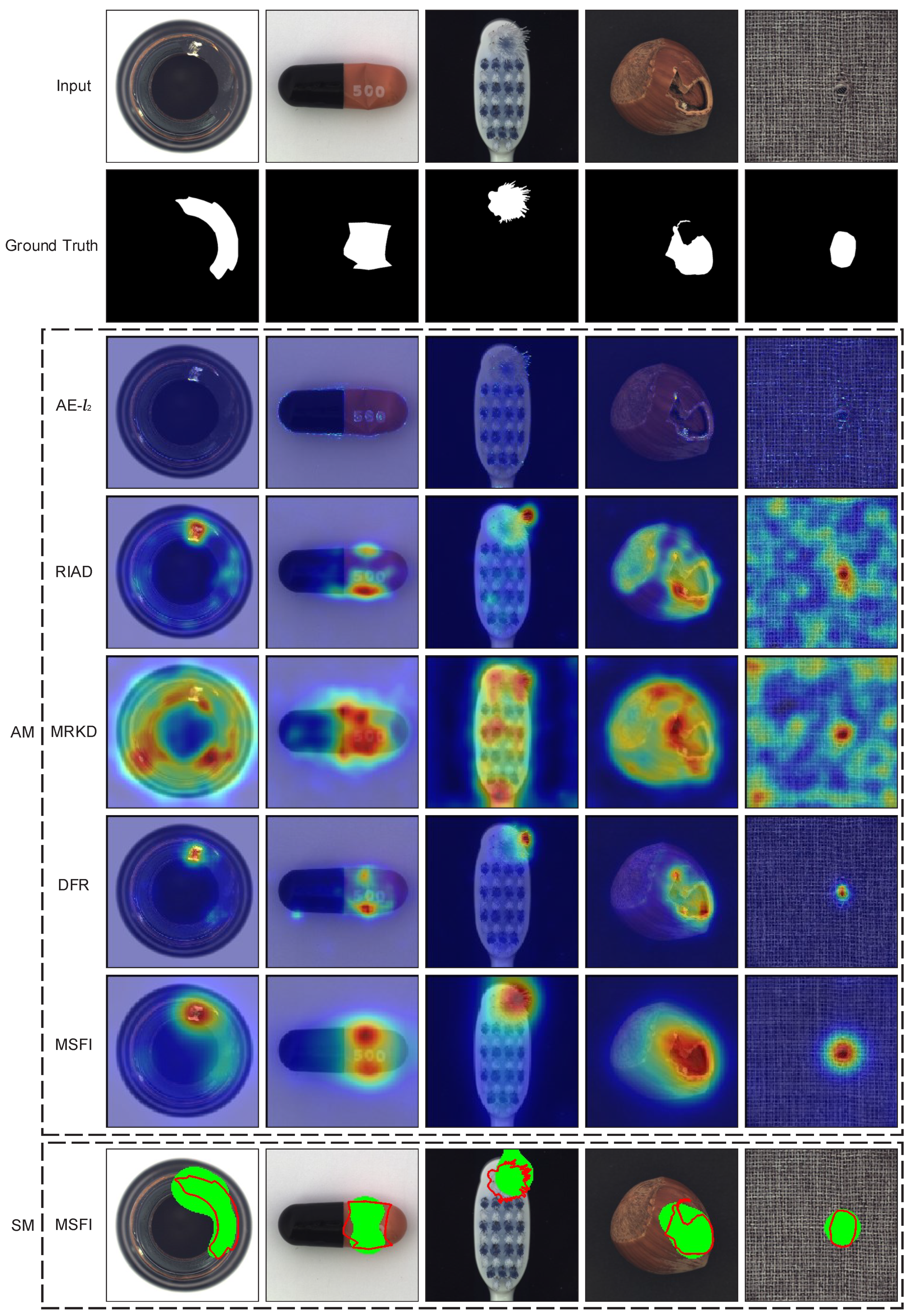
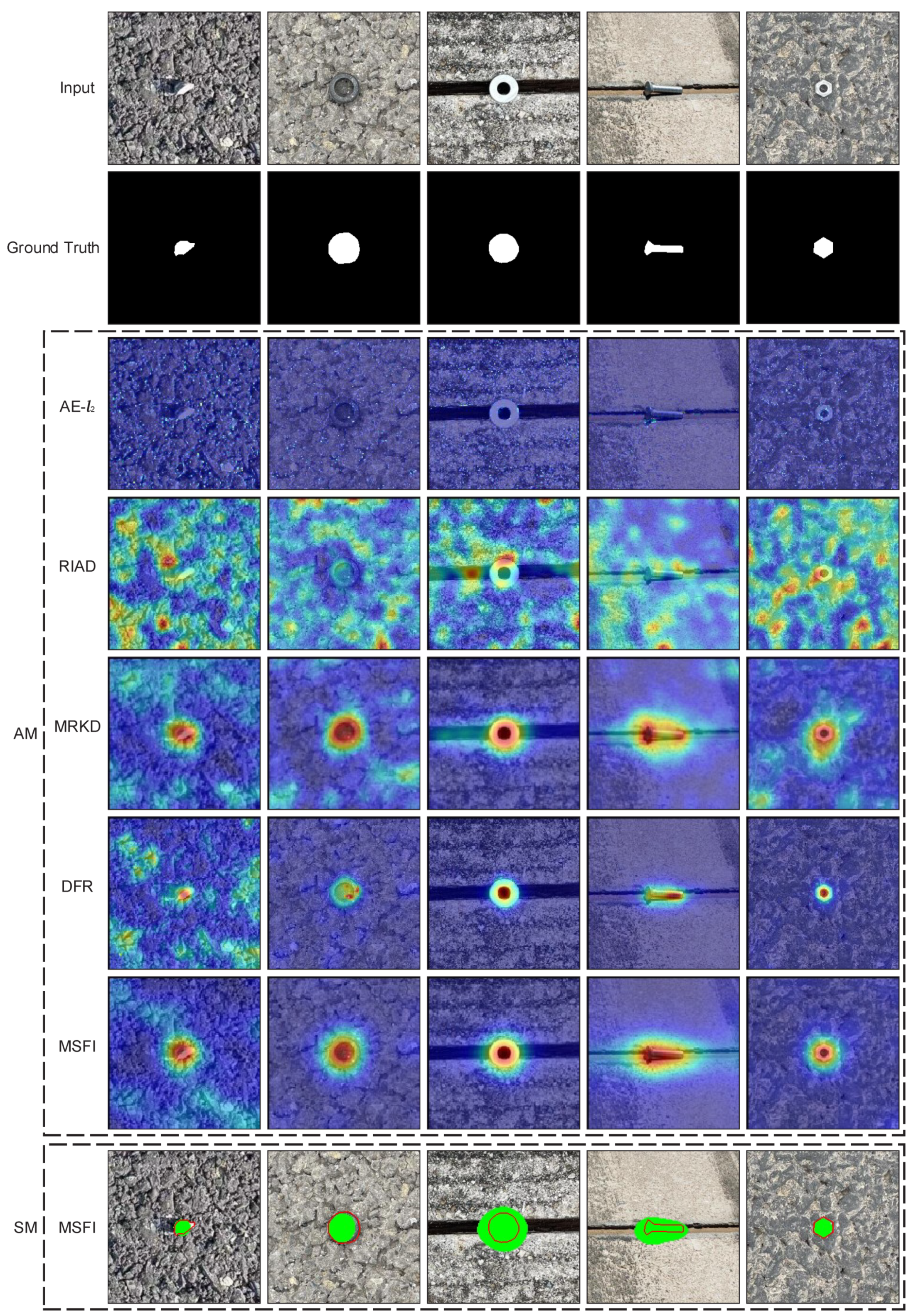
The qualitative comparison between MSFI and other methods on the MVTec AD and FOD datasets is visualized in Figure 5 and Figure 6, which show the anomaly maps of both methods and the segmentation maps of MSFI. For visualization, the anomaly map is normalized to the range of [0,1], and then superimposed on corresponding testing images. It can be observed that MSFI generally produces more reasonable anomaly maps compared with other methods. The reconstruction error is low for normal regions and high for abnormal regions, reducing the incorrect classification of normal regions and missing detection of abnormal regions. Visually, MRKD, DFR and MSFI can capture abnormal regions in images more accurately than AE-$l_2$ and RIAD based on image reconstruction. This may be because the former adopts the pre-trained features that can bolster their pattern-recognition abilities. This indicates that the method using pre-trained CNN is better for image anomaly detection than the method of learning image representation from scratch.

6. Ablation Studies

6.1. Effectiveness of Multi-Scale Features

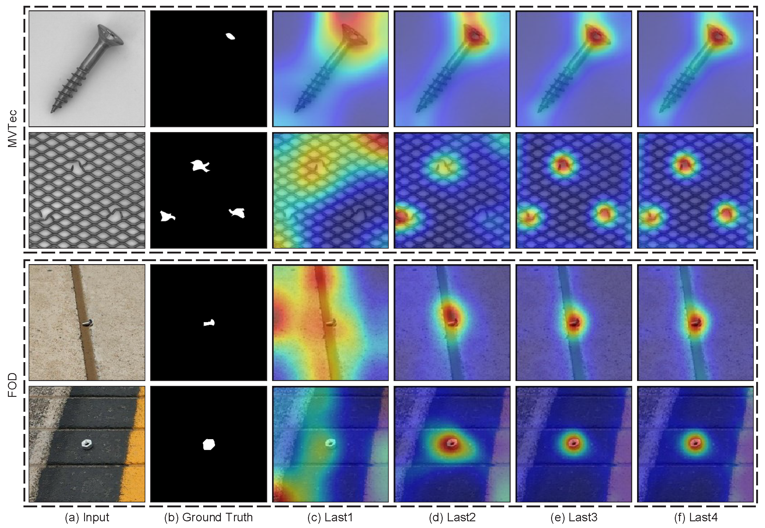
This study adopts a series of different hierarchical features (that is, the last, the last two, the last three and the last four convolution blocks) to construct the model. The effectiveness of the models with different hierarchical features is evaluated on MVTec AD and FOD datasets, and the results are shown in

Table 5. The results of MSFI on the MVTec AD and FOD datasets with different hierarchical features. Image-level AUROC represents the average AUROC of all the classes for anomaly detection. Pixel-level AUROC represents the average AUROC of all the classes for anomaly localization.

Category	Metric	Last1	Last2	Last3	Last4
MVTec AD	Image-level AUROC	0.828	0.905	0.944	0.949
	Pixel-level AUROC	0.822	0.910	0.950	0.965
FOD	Image-level AUROC	0.878	0.919	0.984	0.988
	Pixel-level AUROC	0.826	0.908	0.976	0.985

. Obviously, the performance of MSFI becomes better as the number of layers increases.

Figure 7 represents the qualitative results of MSFI with different hierarchical features on MVTec AD and FOD datasets. It can be seen that with the use of more hierarchical features, the regions that are incorrectly detected as anomalies gradually decrease, and the predicted abnormal regions gradually approach the real abnormal regions. This is because the deep features with more hierarchical features will encode more local details and spatial context information for images, thus making the detection more robust and accurate.

6.2. Loss Function

This section analyzes the impact of each loss component on MSFI.

Table 6. The results of MSFI using different loss functions on the MVTec AD and FOD datasets.

Category	Metric	${\mathit{L}}_{\mathit{dir}}$	${\mathit{L}}_{\mathit{val}}$	${\mathit{L}}_{\mathit{total}}$
MVTec AD	Image-level AUROC	0.835	0.934	0.949
	Pixel-level AUROC	0.863	0.949	0.965
FOD	Image-level AUROC	0.956	0.967	0.988
	Pixel-level AUROC	0.966	0.976	0.985

represents the average AUROC of all classes for anomaly detection and anomaly localization on the MVTec AD and FOD datasets, respectively. MSFI combining two loss functions performs best, and the results show that the performance of anomaly detection could be improved by considering the directional similarity between feature vectors.

6.3. Grid Size

This part analyzes the impact of the grid size on MSFI. The results of MSFI with a single grid size on the MVTec AD and FOD datasets are shown in

Table 7. The results of MSFI trained and evaluated using a single gird size on the MVTec AD and FOD datasets.

Category	Metric	$\mathit{k}=2$	$\mathit{k}=4$	$\mathit{k}=8$
MVTec AD	Image-level AUROC	0.914	0.936	0.920
	Pixel-level AUROC	0.922	0.952	0.931
FOD	Image-level AUROC	0.948	0.967	0.935
	Pixel-level AUROC	0.936	0.956	0.926

. To evaluate the influence of the grid size, a single grid size is used to train the model in the training stage. The testing set also adopts the single grid size during testing. It can be seen from Table 7 that grid size has a great influence on the detection results. No matter what the grid size is, it is difficult to reconstruct the deep features of abnormal regions. This is because the model must infer deep features of abnormal regions from the surrounding regions, which is more difficult than reconstructing the abnormal regions only by a deep autoencoder.

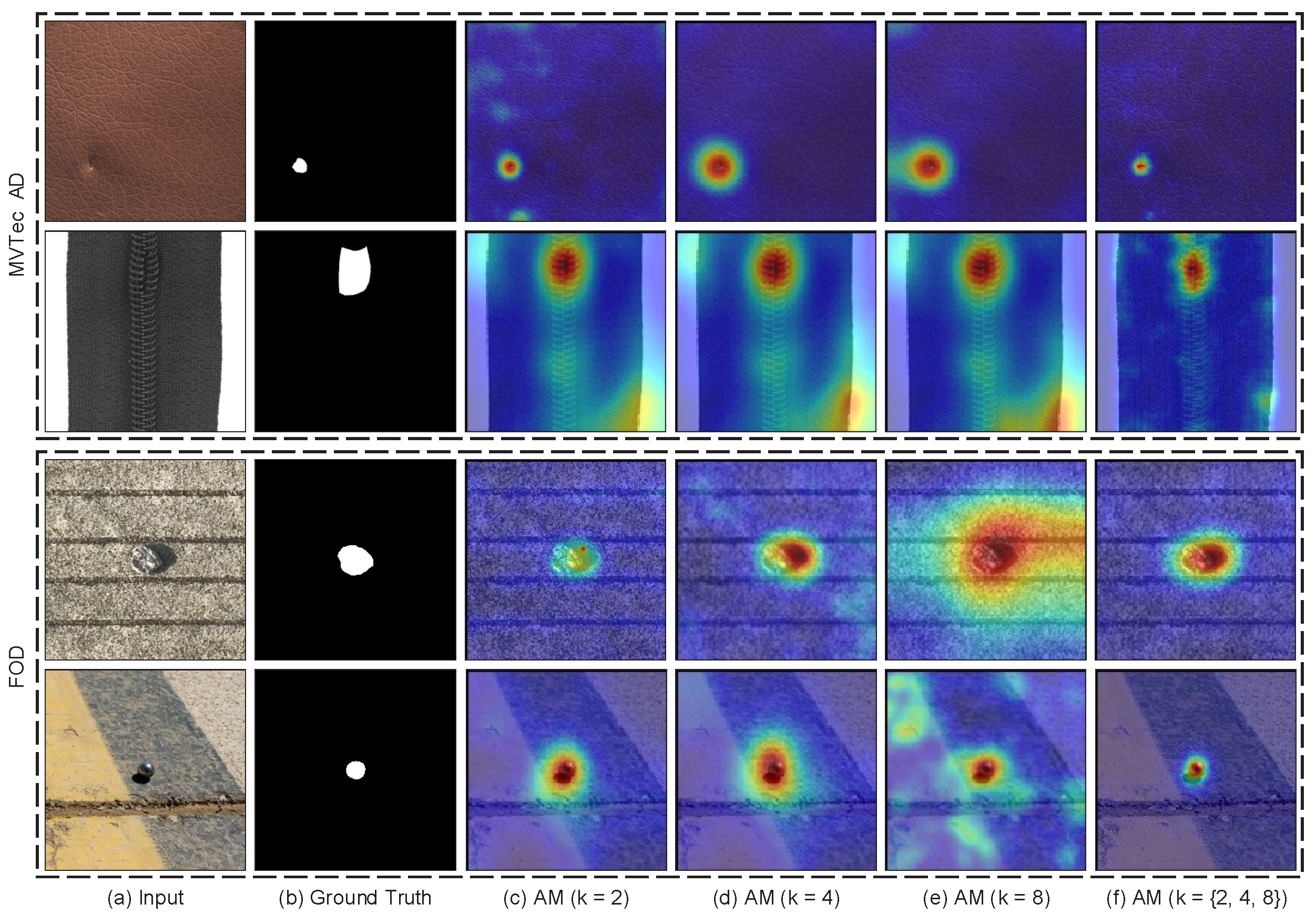
The qualitative results of the model trained using different grid sizes are shown in Figure 8. As the grid size increases, abnormal regions become more difficult to recover and have high anomaly scores. However, normal regions also become difficult to recover and are given high anomaly scores, especially for normal regions with more randomness. As shown in the fourth row of Figure 8, the regions with marker lines in the image produce higher anomaly scores. Adoption of a combination of different grid sizes helps to generate high anomaly scores in abnormal regions and maintain low anomaly scores in normal regions, as shown in column (f) of Figure 8.

7. Discussion

In this study, the current FOD detection methods based on optical images are investigated. The existing FOD detection methods are mainly based on supervised learning, which require massive labeled images. However, since FOD is not clearly defined, the FOD samples cannot be collected comprehensively and easily. Consequently, once the method is applied to a new airport, it would be very time-consuming to collect enough FOD samples. Therefore, the methods based on supervised learning are not suitable for FOD detection. Conversely, the unsupervised anomaly detection methods are introduced to perform FOD detection on pavement images for the first time while requiring no real FOD samples. In this study, the images containing FOD are defined as abnormal images and the images without FOD as normal images. Since real FOD samples are not required in the training phase, the unsupervised anomaly detection methods could quickly adapt to a new airport.

The current anomaly detection methods could be divided into two methods: image reconstruction and feature modeling. The methods based on image reconstruction mainly use an autoencoder to reconstruct an original image to a normal image, making the assumption that anomalous regions would not be reconstructed well. The methods of feature modeling leverage pre-trained features of the normal images to train the model, assuming that the distance between the abnormal image and the normal image is larger than that between the normal pairs in feature space. Although these methods do achieve some success, we propose a much more effective method. Our method combines the pre-trained features and self-supervised learning. According to the comparison experiments, these methods, such as AE-$l_2$, RIAD, MRKD and DFR, raised many false alarms in the regions with pavement defects. The results prove that the proposed method is effective and could better distinguish FOD from pavement defects.

Hundreds of aircraft take off and land in airports every day, which means that the time left for FOD detection and cleanup is extremely little. In order to minimize the interference of FOD detection with airport operations, the detection method needs to guarantee real-time FOD detection. In this paper, the experiments were performed on an Nvidia GeForce RTX 2080 Ti GPU and an Intel I9-9940 [email protected] GHz. As for the anomaly detection phase, the inference of the proposed method takes about 0.07 s per image, and the running speed of MSFI is about 15 fps. As we can see, there is still room for improvement in our method in inference speed, which will be investigated in future work.

8. Conclusions

This study proposes a multi-scale feature inpainting method to perform FOD detection on images with various pavement backgrounds while requiring no real FOD. The pre-trained CNN is fully utilized to establish discriminative multi-scale features for the images. A deep feature inpainting module is designed and trained to learn how to reconstruct the missing region removed by multi-scale grid masks to match normal features. During testing, the abnormal regions, i.e., FOD, are inferred according to the difference between the original feature and its reconstruction version. Furthermore, a new dataset (FOD) containing 9042 airfield pavement images that covers 15 types of FOD is established for FOD detection. Extensive experiments and analysis on the FOD dataset and a public benchmark dataset, MVTec AD, have indicated that the proposed method is effective and outperforms other methods.

References

- Federal Aviation Administration (FAA). Foreign Object Debris (Fod) Management; Document Advisory Circular(ac) 150/5220-24; FAA: Washington, DC, USA, 2010. [Google Scholar]
- Munyer, T.; Huang, P.-C.; Huang, C.; Zhong, X. Fod-a: A dataset for foreign object debris in airports. arXiv 2021, arXiv:2110.03072. [Google Scholar]
- Cao, X.; Wang, P.; Meng, C.; Bai, X.; Gong, G.; Liu, M.; Qi, J. Region based CNN for foreign object debris detection on airfield pavement. Sensors 2018, 18, 737. [Google Scholar] [CrossRef] [PubMed]
- Hu, K.; Cui, D.; Zhang, Y.; Cao, C.; Xiao, F.; Huang, G. Classication of foreign object debris using integrated visual features and extreme learning machine. In CCF Chinese Conference on Computer Vision; Springer: Tianjin, China, 2017; pp. 3–13. [Google Scholar]
- Jing, Y.; Zheng, H.; Lin, C.; Zheng, W.; Dong, K.; Li, X. Foreign object debris detection for optical imaging sensors based on random forest. Sensors 2022, 22, 2463. [Google Scholar] [CrossRef] [PubMed]
- Doğru, A.; Bouarfa, S.; Arizar, R.; Aydoğan, R. Using Convolutional Neural Networks to Automate Aircraft Maintenance Visual Inspection. Aerospace 2020, 7, 171. [Google Scholar] [CrossRef]
- He, K.; Gkioxari, G.; Dollár, P.; Girshick, R. Mask r-cnn. In Proceedings of the 2017 IEEE International Conference on Computer Vision (ICCV), Venice, Italy, 22–29 October 2017; IEEE: Venice, Italy, 2017; pp. 2980–2988. [Google Scholar]
- Redmon, J.; Divvala, S.; Girshick, R.; Farhadi, A. You only look once: Unied, real-time object detection. In Proceedings of the 2016 IEEE Conference on Computer Vision and Pattern Recognition (CVPR), Las Vegas, NV, USA, 27–30 June 2016; IEEE: LasVegas, NV, USA, 2016; pp. 77–788. [Google Scholar]
- Yang, Y.; Gong, H.; Wang, X.; Sun, P. Aerial target tracking algorithm based on faster r-cnn combined with frame differencing. Aerospace 2017, 4, 32. [Google Scholar] [CrossRef]
- Chalapathy, R.; Chawla, S. Deep learning for anomaly detection: A survey. arXiv 2019, arXiv:1901.03407. [Google Scholar]
- Pang, G.; Shen, C.; Cao, L.; Hengel, A.V.D. Deep learning for anomaly detection: A review. ACM Comput. 2021, 54, 38. [Google Scholar] [CrossRef]
- Luo, Z.; He, K.; Yu, Z. A robust unsupervised anomaly detection framework. Appl. Intell. 2022, 52, 6022–6036. [Google Scholar] [CrossRef]
- Park, H.; Noh, J.; Ham, B. Learning memory-guided normality for anomaly detection. In Proceedings of the 2020 IEEE/CVF Conference on Computer Vision and Pattern Recognition (CVPR), Seattle, WA, USA, 13–19 June 2020; IEEE: Seattle, WA, USA, 2020; pp. 14360–14369. [Google Scholar]
- An, J.; Cho, S. Variational autoencoder based anomaly detection using reconstruction probability. Spec. Lect. IE 2015, 2, 1–18. [Google Scholar]
- Cohen, N.; Hoshen, Y. Sub-image anomaly detection with deep pyramid correspondences. arXiv 2020, arXiv:2005.02357. [Google Scholar]
- Rippel, O.; Mertens, P.; König, E.; Merhof, D. Gaussian anomaly detection by modeling the distribution of normal data in pretrained deep features. IEEE Trans. Instrum. Meas. 2021, 70, 1–13. [Google Scholar] [CrossRef]
- Wan, Q.; Gao, L.; Li, X.; Wen, L. Industrial image anomaly localization based on gaussian clustering of pretrained feature. IEEE Trans. Ind. Electron. 2022, 69, 6182–6192. [Google Scholar] [CrossRef]
- Bergmann, P.; Fauser, M.; Sattlegger, D.; Steger, C. Mvtec ad a comprehensive real-world dataset for unsupervised anomaly detection. In Proceedings of the 2019 IEEE/CVF Conference on Computer Vision and Pattern Recognition (CVPR), Long Beach, CA, USA, 15–20 June 2019; IEEE: Long Beach, CA, USA, 2019; pp. 9584–9592. [Google Scholar]
- Bergmann, P.; Löwe, S.; Fauser, M.; Sattlegger, D.; Steger, C. Improving unsupervised defect segmentation by applying structural similarity to autoencoders. arXiv 2018, arXiv:1807.02011. [Google Scholar]
- Qin, K.; Wang, Q.; Lu, B.; Sun, H.; Shu, P. Flight Anomaly Detection via a Deep Hybrid Model. Aerospace 2022, 9, 329. [Google Scholar] [CrossRef]
- Kingma, D.P.; Welling, M. Auto-encoding variational bayes. In Proceedings of the 2nd International Conference on Learning Representations (ICLR), Banff, AB, Canada, 14–16 April 2014; pp. 9584–9592. [Google Scholar]
- Memarzadeh, M.; Matthews, B.; Avrekh, I. Unsupervised Anomaly Detection in Flight Data Using Convolutional Variational Auto-Encoder. Aerospace 2020, 7, 115. [Google Scholar] [CrossRef]
- Hou, J.; Zhang, Y.; Zhong, Q.; Xie, D.; Pu, S.; Zhou, H. Divideand-assemble: Learning block-wise memory for unsupervised anomaly detection. In Proceedings of the 2021 IEEE/CVF International Conference on Computer Vision (ICCV), Montreal, BC, Canada, 11–17 October 2021; IEEE: Montreal, QC, Canada, 2021; pp. 8771–8780. [Google Scholar]
- Gong, D.; Liu, L.; Le, V.; Saha, B.; Mansour, M.R.; Venkatesh, S.; Van Den Hengel, A. Memorizing normality to detect anomaly: Memoryaugmented deep autoencoder for unsupervised anomaly detection. In Proceedings of the 2019 IEEE/CVF International Conference on Computer Vision (ICCV), Seoul, Korea, 27 October–2 November 2019; IEEE: Seoul, Korea, 2019; pp. 1705–1714. [Google Scholar]
- Goodfellow, I.J.; Pouget-Abadie, J.; Mirza, M.; Xu, B.; Warde-Farley, D.; Ozair, S.; Courville, A.; Bengio, Y. Generative adversarial nets. In Proceedings of the 27th International Conference on Neural Information Processing Systems, Montreal, BC, Canada, 8–13 December 2014; MIT Press: Cambridge, MA, USA, 2014; pp. 2672–2680. [Google Scholar]
- Schlegl, T.; Seeböck, P.; Waldstein, S.M.; Schmidt-Erfurth, U.; Langs, G. Unsupervised anomaly detection with generative adversarial networks to guide marker discovery. In Information Processing in Medical Imaging; Springer: Cham, Switzerland, 2017; pp. 146–157. [Google Scholar]
- Li, Z.; Li, N.; Jiang, K.; Ma, Z.; Wei, X.; Hong, X.; Gong, Y. Superpixel masking and inpainting for self-supervised anomaly detection. In Proceedings of the 31st British Machine Vision Conference 2020, (BMVC), Cardiff, UK, 7–10 September 2020; BMVA Press: Cardiff, UK, 2020; pp. 7–10. [Google Scholar]
- Yan, X.; Zhang, H.; Xu, X.; Hu, X.; Heng, P.-A. Learning semantic context from normal samples for unsupervised anomaly detection. In Proceedings of the AAAI Conference on Articial Intelligence, Virtual, 2–9 February 2021; AAAI Press: Palo Alto, CA, USA, 2021; pp. 3110–3118. [Google Scholar]
- Ruff, L.; Vandermeulen, R.A.; Franks, B.J.; Müller, K.-R.; Kloft, M. Rethinking assumptions in deep anomaly detection. arXiv 2020, arXiv:2006.00339. [Google Scholar]
- Liznerski, P.; Ruff, L.; Vandermeulen, R.A.; Franks, B.J.; Kloft, M.; Müller, K.-R. Explainable deep one-class classication. arXiv 2020, arXiv:2007.01760. [Google Scholar]
- Salehi, M.; Sadjadi, N.; Baselizadeh, S.; Rohban, M.H.; Rabiee, H.R. Multiresolution knowledge distillation for anomaly detection. In Proceedings of the 2021 IEEE/CVF Conference on Computer Vision and Pattern Recognition (CVPR), Nashville, TN, USA, 20–25 June 2021; IEEE: Nashville, TN, USA, 2021; pp. 14897–14907. [Google Scholar]
- Wang, S.; Wu, L.; Cui, L.; Shen, Y. Glancing at the patch: Anomaly localization with global and local feature comparison. In Proceedings of the 2021 IEEE/CVF Conference on Computer Vision and Pattern Recognition (CVPR), Nashville, TN, USA, 20–25 June 2021; IEEE: Nashville, TN, USA, 2021; pp. 254–263. [Google Scholar]
- Ruff, L.; Vandermeulen, R.; Goernitz, N.; Deecke, L.; Siddiqui, S.A.; Binder, A.; Müller, E.; Kloft, M. Deep one-class classication. In Proceedings of the International Conference on Machine Learning, Stockholm, Sweden, 10–15 July 2018; pp. 4393–4402. [Google Scholar]
- Yi, J.; Yoon, S. Patch svdd: Patch-level svdd for anomaly detection and segmentation. In Computer Vision—ACCV 2020; Springer: Cham, Switzerland, 2021; pp. 375–390. [Google Scholar]
- Bergmann, P.; Fauser, M.; Sattlegger, D.; Steger, C. Uninformed students: Student-teacher anomaly detection with discriminative latent embeddings. In Proceedings of the 2020 IEEE/CVF Conference on Computer Vision and Pattern Recognition (CVPR), Seattle, WA, USA, 13–19 June 2020; IEEE: Seattle, WA, USA, 2020; pp. 4182–4191. [Google Scholar]
- He, K.; Zhang, X.; Ren, S.; Sun, J. Deep residual learning for image recognition. In Proceedings of the 2016 IEEE Conference on Computer Vision and Pattern Recognition (CVPR), Las Vegas, NV, USA, 27–30 June 2016; IEEE: Las Vegas, NV, USA, 2016; pp. 770–778. [Google Scholar]
- Ronneberger, O.; Fischer, P.; Brox, T. U-net: Convolutional networks for biomedical image segmentation. In International Conference on Medical Image Computing and Computer-Assisted Intervention; Springer: Cham, Switzerland, 2015; pp. 234–241. [Google Scholar]
- Simonyan, K.; Zisserman, A. Very deep convolutional networks for largescale image recognition. arXiv 2014, arXiv:1409.1556. [Google Scholar]
- Deng, J.; Dong, W.; Socher, R.; Li, L.-J.; Li, K.; Li, F.-F. Imagenet: A large-scale hierarchical image database. In Proceedings of the 2009 IEEE Conference on Computer Vision and Pattern Recognition, Miami, FL, USA, 20–25 June 2009; IEEE: Miami, FL, USA, 2009; pp. 248–255. [Google Scholar]
- Zavrtanik, V.; Kristan, M.; Skočaj, D. Reconstruction by inpainting for visual anomaly detection. Pattern Recognit. 2021, 112, 107706. [Google Scholar] [CrossRef]
- Shi, Y.; Yang, J.; Qi, Z. Unsupervised anomaly segmentation via deep feature reconstruction. Neurocomputing 2021, 424, 9–22. [Google Scholar] [CrossRef]
Figure 1.
The overview of the multi-scale feature inpainting (MSFI). It consists of four parts: multi-scale feature generation, multi-scale grid masks, deep feature inpainting and anomaly detection and localization.
Figure 2.
Visualization of the multi-scale grid masks.
Figure 3.
Examples of normal and abnormal images for each class on MVTec AD dataset. For each class, the top row shows normal image, and the bottom abnormal image.
Figure 4.
Examples of normal and abnormal images for each class on FOD dataset. For each class, the top row shows normal images without FOD, and the bottom shows abnormal images with FOD.
Figure 5.
Qualitative comparison between the proposed method and other methods on MVTec AD dataset. Input represents the input abnormal image. Ground Truth represents the actual abnormal regions (in white). AM represents the anomaly map. SM represents the segmentation map. The red region represents the high anomaly score of AM, the solid red line indicates the boundary of the actual abnormal region and the green region represents the predicted abnormal region in SM.
Figure 6.
Qualitative comparison between the proposed method and other methods on FOD dataset. Input represents the input abnormal image. Ground Truth represents the actual abnormal regions (in white). AM represents the anomaly map. SM represents the segmentation map. The red region represents the high anomaly score of AM, the solid red line indicates the boundary of the actual abnormal region and the green region represents the predicted abnormal region in SM.
Figure 7.
Qualitative results of MSFI with increasing hierarchical features on the MVTec AD and FOD datasets. Last l: anomaly map of MSFI using the hierarchical features from the last l convolution blocks.
Figure 8.
Qualitative results of MSFI trained and evaluated on a single gird size on the MVTec AD and FOD datasets. AM (), AM () and AM () respectively represent the anomaly map of MSFI trained with a single grid sizes of 2, 4 and 8. AM () represents the anomaly map of MSFI trained and evaluated on the set .