An Approach for the Simulation of Ground and Honed Technical Surfaces for Training Classifiers

Abstract

Training of neural networks requires large amounts of data. Simulated data sets can be helpful if the data required for the training is not available. However, the applicability of simulated data sets for training neuronal networks depends on the quality of the simulation model used. A simple and fast approach for the simulation of ground and honed surfaces with predefined properties is being presented. The approach is used to generate a diverse data set. This set is then applied to train a neural convolution network for surface type recognition. The resulting classifier is validated on the basis of a series of real measurement data and a classification rate of >85% is achieved. A possible field of application of the presented procedure is the support of measurement technicians in the standard-compliant evaluation of measurement data by suggestion of specific data processing steps, depending on the recognized type of manufacturing process.

1. Introduction

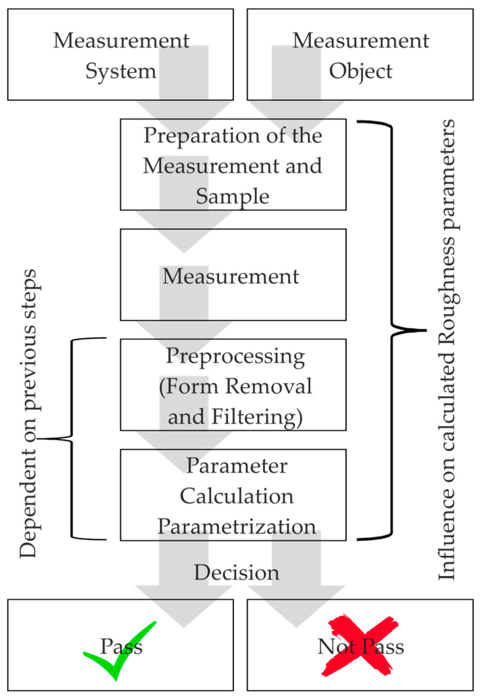
Production metrology deals with all of the measuring and inspection tasks that arise during the creation of products. Usually, function-related characteristics of workpieces are measured. In addition to the measurement, the procedure for evaluating surface roughness (e.g., 3D) as a quality criterion includes the steps of data preprocessing (e.g., filtering [1]) and parameter calculation [2] (cf. Figure 1). A large number of parameters exist for standard-compliant data preprocessing, as well as for standard-compliant roughness parameters calculation [2,3,4]. The selection of standard-compliant parameters has to be done manually and can be a challenge. In the case of recurring, identical measurement tasks, an expert defines the data processing steps once for all similar measurements. However, since a measuring device is usually used for a large number of different and changing measuring tasks, the parameterization of the measurement data processing steps must be adapted by the operator repeatedly. In the case of unknown or incorrectly assumed boundary conditions (e.g., due to communication errors, when measurements and evaluations are carried out by different persons), there is a risk that steps of the measurement data processing will be changed or incorrectly parameterized, and that the determined parameters are thus incorrect or no longer comparable.

Assistance software, developed for example in the project “OptAssyst—User-oriented assistance systems for the safe use of optical distance sensors” funded by the German Federal Ministry of Education and Research (BMBF) [5] supports the user in the selection of the measuring principle, as well as in the parameterization of the data processing [6,7]. However, for the standard-compliant evaluation of surface roughness, the complete measuring task must be known, which includes knowledge of the manufacturing process. As an example, the surface filter must be selected in such a way that the surface details like e.g., grooves are not distorted—i.e., linear filters [3] for ground surfaces and robust filters for plateau-honed surfaces [4].

In order to support the user, it is therefore useful to automatically classify the measurement object and the related manufacturing process in order to suggest a standard-compliant procedure for measurement data processing and evaluation.

Signal processing approaches, which are usually used for the characterization of technical surfaces, such as radon transformation [8] or the watershed transformation [9], offer a solution for realizing classifiers. Parameters derived from these transformations, such as the number and location of peaks in the radon transformation, can be used for classification. However, the implementation of such approaches can be impractical for a non-expert user, as it requires extensive knowledge of both signal processing and the process. Another challenge is the extension of pre-selected transformational-based classifiers to other surface types.

Artificial neural networks (ANN) are an approach to the implementation of classifiers based only on measurement data sets and are therefore an alternative to signal processing approaches. Specifically convolutional neural networks (CNN) are successfully used to classify images, for example for the recognition of handwriting [10] or for recognizing objects in images [11]. On the one hand, this success leads to further research and new discoveries, such as Generative Adversarial Networks [12], for manipulating neuronal networks or the “deconvnet” for visualizing neuronal networks [13]. On the other hand, the success results in tools that make the application of CNN easier. Since surfaces measured with topography measuring instruments (such as Confocal microscopy, Coherence scanning interferometry), which deliver 2.5D elevation maps can be interpreted as grayscale images, the transfer of these techniques is evident. However, since the training of CNN requires a large amount of data (>1000 measurements), which is not always available, artificially generated measurement data sets with specific properties of technical surfaces are of interest. Therefore, an approach for generating two different classes of technical surfaces with predefined properties is presented (ground and honed surfaces). This artificial data is then used to train a simple convolutional neuronal network for surface classification. In the next step, the classifier that was trained with artificial data is verified by means of real measurement data sets (honed cylinder liners of different car manufacturers and a selection of ground surfaces).

The classification task with only two classes was deliberately chosen in such a way that the proposed procedure can be tested easily. Future work, which is excluded from this paper, focuses on the generation of optimal input data for artificial surface models based on time series models estimation from small sets of actual measurement data, and the application of more advanced or complex neuronal networks.

2. Approach for the Generation of Artificial Ground and Honed Surfaces

Real technical surfaces often have stochastically distributed features. The structure of those features depends on the chosen manufacturing process. In grinding or honing processes, geometrically indefinite cutting edges are used. Plasma-coated surfaces contain stochastically distributed pores. In many different applications, mathematical models for the simulation of such surfaces already exist.

The probability distribution of the topography heights is often assumed as Gaussian [14,15,16]. For honed surfaces, this assumption is invalid. Their probability distribution is often strongly asymmetric [17,18,19,20,21,22,23]. Existing models for the simulation of honed surfaces aim to produce surfaces with identical properties (e.g., roughness parameters) as given real surfaces. For the approach chosen in this paper, the objective is different: The aim is to simulate many different surfaces with the same (default) character, but the exact properties should be distributed stochastically.

A honing process can be seen as a modification of a grinding process. The movement of the honing stones relative to the surface leads to the characteristic cross-structure with the honing angle α. The probability distribution of the topography heights in a grinding process can be assumed as Gaussian. With multi-step honing processes (e.g., plateau honing), surfaces with a shallow peak area and a distinct valley area can be created. Hence, the different honing steps can be simulated as Gaussian topographies [24,25]. The combination of those topographies results in the final surface. A comparable approach was chosen in [21]. The model for the simulation of the Gaussian topographies is based on the approaches of [18,26]. The 2.5D topographies can be described as matrices of the form:

$$z_{i,j}=z\left(x_i,y_j\right),i=0,\dots ,M-1,j=0,\dots ,N-1,$$

(1)

The point distance in direction of the x-axis is referred to as Δx and in y as Δy. The lateral properties of the surface are described with the circular autocorrelation function:

$$R_{k,l}^{\ast }=\frac{1}{MN}{\displaystyle \sum _{m=0}^{M-1}{\displaystyle \sum _{n=0}^{N-1}{z}_{m,n}}{z}_{m+k,n+l}},0\le k\le M-1,0\le l\le N-1,$$

(2)

With $z_{m+k,n+l}=z_{m+k-M,n+l}$ for m + k > M – 1 $\wedge$ n + l ≤ N – 1, analogous for n + l > N – 1 and combinations. The discrete power spectral density is the Fourier transform of the autocorrelation function:

$$S_{p,q}^{\ast }=\frac{1}{MN}{\displaystyle \sum _{m=0}^{M-1}{\displaystyle \sum _{n=0}^{N-1}{R}_{m,n}^{\ast }\exp \left(-i\cdot 2\pi \left[\frac{mp}{M}+\frac{nq}{N}\right]\right)}},$$

(3)

The aim is to generate a discrete 3D-Topography of the form:

$$z=\left(z_{k,l}\right)=\left(z\left(x_k,y_l\right)\right),0\le k\le M-1,0\le l\le N-1,$$

(4)

With $x_k=k\cdot \Delta x$, $0\le k\le M-1$, $y_l=l\cdot \Delta y$, $0\le l\le N-1$. The input data for the simulation is: A circular autocorrelation function $R_{k,l}^{\ast },0\le k\le M-1,0\le l\le N-1$, respectively its Fourier transform (the discrete power spectral density) $S_{p,q}^{\ast },0\le p\le M-1,0\le q\le N-1$, a matrix $g=\left(g_{k,l}\right)=\left(g\left(x_k,y_l\right)\right)$ with standard normal distributed entries and the variance ${\sigma }_{tar}^2(z)$ of the target surface. The given autocorrelation function must not contain phases; the corresponding discrete power spectral density must be real. Otherwise, $S_{p,q}^{\ast }=\left|S_{p,q}^{\ast }\right|$ is set for the simulation. This changes the shape of the autocorrelation function. The Fourier transform of the matrix g is G = F(g), so that:

$$G_{p,q}=\frac{1}{MN}{\displaystyle \sum _{m=0}^{M-1}{\displaystyle \sum _{n=0}^{N-1}{g}_{m,n}\exp \left(-i\times 2\pi \left[\frac{mp}{M}+\frac{nq}{N}\right]\right)}},$$

(5)

The 2.5D-topography $z=\left(z_{k,l}\right)$ is generated from the input data with:

$$z_{k,l}={\displaystyle \sum _{r=0}^{M-1}{\displaystyle \sum _{s=0}^{N-1}\sqrt{S_{r,s}^{\ast }}{G}_{r,s}}}\exp \left(-i\times 2\pi \left[\frac{rk}{M}+\frac{sl}{N}\right]\right),$$

(6)

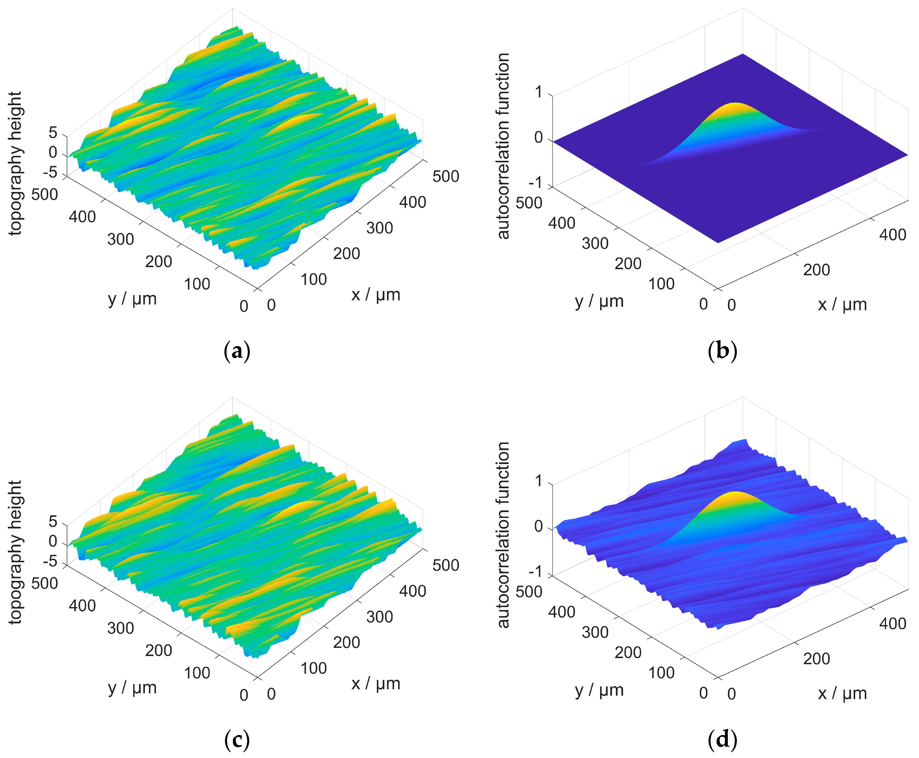
The Fourier transform of g is convoluted with the square root of the given power spectral density in the frequency domain. To achieve the requested variance ${\sigma }_{tar}^2(z)$, the power spectral density has to be normalized. The simulation method used here is similar to the one presented by Wu [26]. Wu uses a complex vector with uniformly distributed phases and constant amplitude instead of the Fourier transform G of a normal distributed matrix g. With such an approach, the given autocorrelation function is exactly mapped into the simulated topographies e.g., it does not contain any stochastic variations as in the approach chosen for this paper (cf. Figure 2b,d)). The difference in the generated artificial surfaces is subtle (cf. Figure 2a,c).

However, since the model presented here is intended to simulate the stochastic properties of real surface topographies, this aspect should also be taken into account. In order to illustrate the difference between the two methods, definitions from the next paragraph are already used here. The autocorrelation function used in this example is the function R(x,y), defined in the next paragraph with parameters l₁ = 100 µm, l₂ = 5 µm, a = 2, and ${\sigma }^2$ = 1 µm. Δx and Δy are chosen as 0.5 µm, the size of the simulated surface is 1000 × 1000 points.

3. Simulation of Directional Structures (Grinding Surfaces)

The autocorrelation function of real technical surfaces is approximately an exponential function [6]. A more general model is chosen for the simulation:

$$\tilde{R}\left(x,y\right)=e^{-\left({\left|\frac{\cos \left(\phi \right)\cdot x+sin\left(\phi \right)\cdot y}{l_1}\right|}^a+{\left|\frac{sin\left(\phi \right)\cdot x+\cos \left(\phi \right)\cdot y}{l_2}\right|}^a\right)},$$

(7)

Here, the exponent a determines the character of the autocorrelation function. For a = 1, its shape is exponential and for a = 2 it is Gaussian. The autocorrelation function is not necessarily orthogonal to the axes of coordinates, therefore the angle $\phi$ is introduced. It specifies the rotation of the autocorrelation function around the origin and corresponds to the main direction of the structures respectively. the honing angle. The parameters l₁ and l₂ are the correlation lengths in direction $\phi$ and $\phi +90°$. The correlation length describes the distance, where the standardized autocorrelation function falls to h = e⁻¹. In literature, other definitions for h exist, e.g., h = 0.2 [1]. The continuous autocorrelation function $\tilde{R}\left(x,y\right)$ is discretized and used as a circular autocorrelation function. Depending on the parameter selection, non-differentiable points and discontinuities might occur, and the associated power spectral density may not be real. In the simulation, this leads to deviations from the requested autocorrelation function. Those deviations become smaller, as the simulated topography becomes larger in relation to the chosen autocorrelation length. The parameters for the simulation of a Gaussian distributed surface are the expectation value µ, the variance ${\sigma }^2$, the correlation lengths l₁ and l₂, the exponent a and the angle $\phi$ (cf. Figure 3).

4. Simulation of Honed Structures in Multiple Steps

4.1. One-Step Honing Process

A one-step honing process can be seen as a combination of two grinding processes. The up- and downward movement of the honing tool generates directional structures with an angle $\phi$ and $-\phi$. Together they generate the characteristic cross-structure. Both processes remove material, so the result for a one-step honing process is:

$$z_h\left(x,y,l_x,l_y,\phi ,\sigma ,\mu \right)=\min \left(z_{s+},z_{s-}\right),$$

(8)

where $z_{s+}$ and $z_{s-}$ are two simulated, Gaussian distributed topographies with the same simulation parameters. The angles are $\phi$ for $z_{s+}$ and $-\phi$ for $z_{s-}$. The exponent, a, is chosen as 2 (Gaussian), if not marked otherwise (see Figure 4a). It should be considered that µ and $\sigma$ are parameters of the two Gaussian distributed topographies and do not represent the expectation value and the standard distribution of the simulated honing process. The probability distribution of the honing process is the probability distribution of the minimum of two Gaussian distributed random variables and therefore not a Gaussian distribution.

4.2. Multi-Step Honing Processes

For the simulation of a multi-step honing process, multiple simulated one-step honing processes are combined. One process virtually removes material from the topography resulting from the previous steps. Mathematically, the resulting topography is the minimum of multiple one-step honing topographies

$$z_h^n=\min \left(z_{h,1},z_{h,2},\dots ,z_{h,n}\right),$$

(9)

The different processes $z_{h,i}$ are differently parameterized. In general, two simulated honing processes are sufficient to reproduce the structure of a plateau honed surface (cf. Figure 4b).

5. Approach for the Classification of Simulated Ground and Honed Surfaces Using Machine Learning

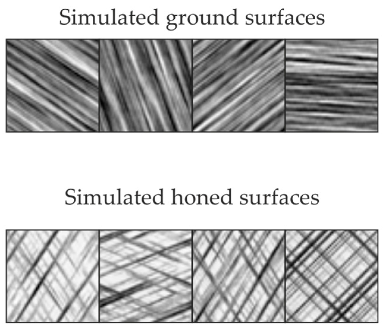
The techniques described above can be used for the fast generation of artificial data sets with defined characteristics. Here, a total of 2000 ground and honed surfaces were simulated, of which 1000 were selected for training the network and 1000 as test data sets. The parameters used for generation are given in

Table 1. Selected parameters for generating the training and test data. For parameters with a range, a uniform distribution over the range is assumed.

Parameter	Value
General parameters
Δx	0.5 µm
Δy	0.5 µm
nx	500
ny	500
a	2
Parameters for ground surfaces simulation
l1	400 ± 100 µm
l2	5 ± 0.8 µm
${\sigma }^2$	22 ± 3
$\phi$	90 ± 90° (integer steps)
Parameters for honed surfaces simulation
l1 (first processing step)	500 ± 200 µm
l2 (first processing step)	30 ± 10 µm
l1 (2nd processing step)	5 ± 1 µm
l2 (2nd processing step)	3 ± 1 µm
µ1	0 µm
µ2	0 µm
${\sigma }_1^2$	45 ± 5
${\sigma }_2^2$	0.2 ± 0.1
${\phi }_1$, ${\phi }_2$	45 ± 25° (integer steps)

. The measurement field size (500 × 500 pixels) was selected in such a way that it is in the range of typical confocal microscopes (e.g., NanoFocus µSurf explorer: measurement field 512 × 512 pixels). For the grinding structures, the lateral point distances Δx and Δy, and the autocorrelation lengths l₁ and l₂ were selected in order to create the process-specific directed structures. The angle, $\phi$, varies freely. For honed structures, the correlation lengths l₁ and l₂ and variances ${\sigma }_1^2$ and ${\sigma }_2^2$ were chosen in such a way that they correspond to a coarse and a fine process step, similar to plateau honing. The honing angle $\phi$ was varied in a wide range. The simulated data was converted into grayscale images and compressed to 50 × 50 pixels to reduce the computational effort. Examples of the simulated ground and honed surfaces used for training can be found in Figure 5.

The Convolutional Neural Networks (CNNs) were implemented with The Mathworks’ Neural Network Toolbox to classify the simulated test data [27,28,29]. Two architectures, each with two different configurations were tested:

• A two-layer CNN with 8 filters of the size 5 × 5 in the first layer and 4 filters of the size 10 × 10.
• A two-layer CNN with 6 filters of the size 5 × 5 in the first layer and 6 filters of the size 5 × 5.
• A three-layer CNN with 8 filters of the size 5 × 5 in the first layer and 4 filters of the size 5 × 5 in the 2nd and third layer.
• A three-layer CNN with 6 filters of size 5 × 5 in the first, second and third layer.

The convolutional filters that form the core in the CNNs are convolutional operators of a given size (5 × 5 or 10 × 10) similar to edge detectors in image processing. Their weights are initialized randomly and iteratively changed (trained) over multiple epochs. The filter sizes are chosen small, since the structures to be learned by the CNN are expected to be small and primitive (straight lines or edges). The low number of layers (two or three) is due to the fact that the structures occurring in the data are of a periodic nature and do not have to be assembled into more complex structures.

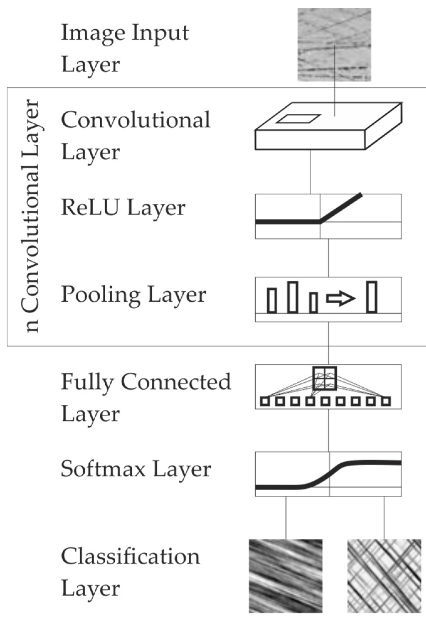
The overall architecture of the investigated neural networks is as follows: An image input layer is used as the first layer to map the input data to the following neurons, followed by the convolutional layers, which consist of the convolution filters, followed by a ReLU layer (rectified linear unit, threshold value operator that assumes the function of an activation function), and a pooling layer, which folds the image with a maximum filter. The combination of convolution, ReLU layer and pooling is expected to preserve important information while reducing the overall data volume, resulting in a reduction of computation time [30]. Following the convolutional layers, a fully connected layer, a softmax layer, and a classification layer is selected (Figure 6).

To train the CNN, the Stochastic Gradient Descend with Momentum [31] is selected. The learning rate is chosen to be 0.01 for the first four epochs and then reduced by 1/10 for every four epochs. For each iteration, 100 simulated surfaces are entered and the maximum number of epochs is limited to eight.

The accuracy of the classification (detection rate) is calculated with:

$$R=\frac{N^{+}}{N},$$

(10)

With N⁺ being the number of correct classified data and N = 2000 the overall data set size.

Both the two-layer CNNs, as well as both three-layer CNNs, are able to distinguish grinded from honed surfaces with decent accuracy after training. For CNN number 1, the accuracy of classification with the artificially generated test set is 96.32%, for case 2 92.55%, for case 3 99.15%, and 99.05% for case 4. Thus, the two three-layer CNNs show a slightly higher classification rate for the artificially generated test data than the two-layer CNNs (see

Table 2. Comparison of the classification performance of the different CNN architectures.

CNN Number	Detection Rate in %
	Simulated Test Data	Real Test Data
1.	96.32	64.88
2.	92.55	84.50
3.	99.15	86.88
4.	99.05	86.88

).

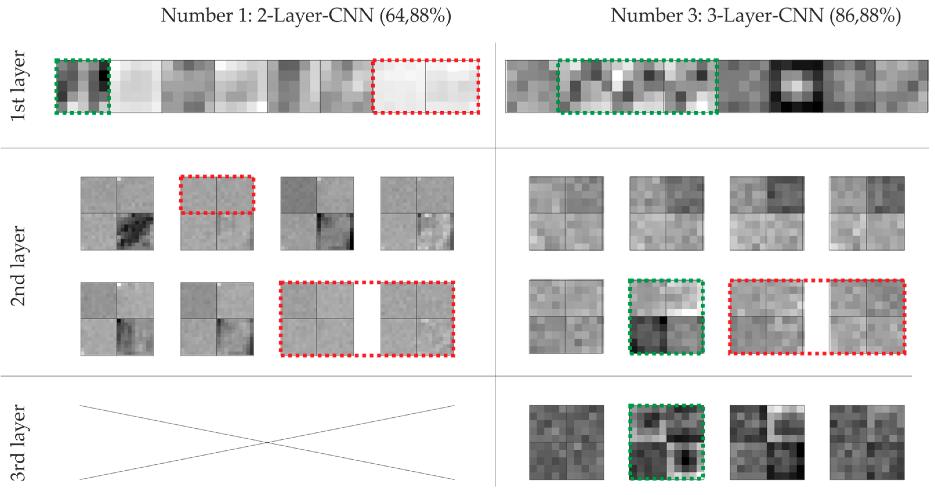
Looking at the weights for the two-layer CNN in the first layer, it is noticeable that edge detection-like structures are visible in the first layer, but they are not directly interpretable (cf. Figure 7, left, 1st row, green). Some of the weights in the first layer, and multiple weights in the 2nd layer appear to be untrained, hence containing noise (cf. Figure 7, left, red). For the three-layer CNN, all of the neurons in the first layer appear to be trained. Three filters appear to have a similar structure (cf. Figure 7, right, 1st row, green). The interpretation of the weights in the 2nd layer is more difficult. Again, some filters appear to be untrained (cf. Figure 7, right, red), while others appear to have a structure. (cf. Figure 5, right, 2nd row, green) The third layer seems to contain mostly trained filters (Figure 7, right, 3rd row, green). A generally visual interpretation of the filter weights is hardly possible.

Generally speaking, the number of untrained filters in CNN structures 1. to 4. indicates that the CNN structure may have been selected too complex for the simple classification task. By adding further surface-types and extending the training set, it can be assumed that these filters will be trained for future characteristics.

6. Verification of the Classifier Using Real Ground and Honed Surfaces

All measurement data used for the verification was acquired as 2.5D-topographies (height maps) during the course of several completed projects not related to this work, using a confocal microscope as measurement device (Nanofocus µSurf explorer, NanoFocus AG, Oberhausen, Germany). This ensures that the existing data is independent of the methodology proposed in the Section 2, Section 3 and Section 4. A selection of honed samples of differently manufactured cylinder liners from various automotive manufacturers from the truck and car sector is used (in total 50 different surfaces, measured in each case at up to 11 different locations, in total 400 records). These are kindly provided by the members of the working group “Arbeitskreis 3D-Rauheitsmesstechnik”. Measured data from real ground surfaces is obtained from the institute’s data archive (in total 400 different measurement data sets) from completed measurement tasks. The real ground surfaces contain data sets with grinding defects.

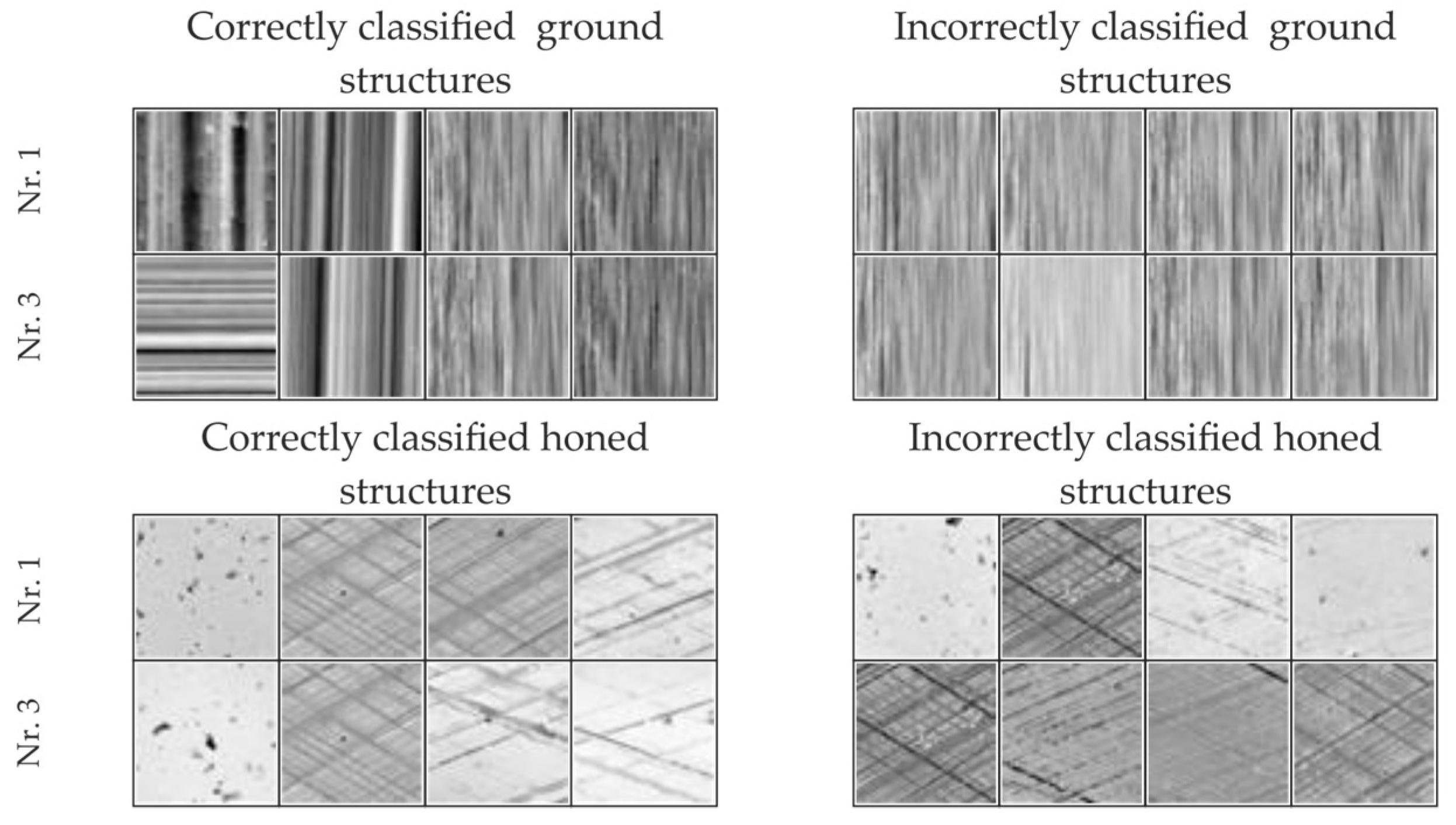
Measurements of the classification performance according to formula 10 of the four different CNN architectures used to distinguish ground and honed surfaces are given in Table 2. The 3-layer CNNs showed better results than the 2-layer CNNs. Both 3-layer CNN architectures classified the same 31 grinding and 74 honing samples incorrectly. What is striking about the incorrectly classified grinding samples is the fact that all of the grinding structures run at an angle of 90°, which hints at a difficulty in learning this specific feature for the classification (cf. Figure 8, top). The wrongly classified honed samples differ in part largely from the average honed surface. Generally, they differ in appearance. There is no obviously visible systematics (cf. Figure 8, bottom). One possible explanation for part of the incorrectly classified data sets is the fact that structures such as pores, which are not considered for the model, occur in the real data sets.

In summary, it can be concluded that the classification rates of over 85% for real measured surfaces are satisfactory as a first result (see Table 2), especially since the verification set contained unmodelled characteristics. However, the detection rate is far from the performance of modern neural networks for more complex tasks [10,30]. Further work is therefore required.

7. Summary and Outlook

A simple approach to the simulation of artificial topographies with the characteristics of ground and honed surfaces was presented. In a second step, the two classes of artificially created surfaces were used to train CNNs in order to recognize the type of surface. It has been shown that simple, modern CNN architectures are suitable for classifying the two simulated surface types. In a third step, the CNNs were used to classify real ground and honed surfaces. The three-layer CNNs showed better results than the two-layer CNNs with a classification rate of above 85%. However, the performance is still below that of state-of-the-art CNNs. The classification task with only two recognizable classes was deliberately chosen as simple in order to test how well neural networks can be implemented and trained.

For the upcoming steps, both the approach to artificial creation of structured surfaces and the CNN for classification will be extended: the input data for the surface creation can be generated from actual measurement data based on stochastic time series models. Based on an optimization approach, ideal models can be chosen that provide the best possible stochastic description of surface properties. The suitability and versatility of this approach will be examined in further studies. It is intended that the resulting CNN can be used to support users in the standard-compliant characterization of technical surfaces through proposals for standard-compliant data processing steps, for example in the calculation of roughness parameters.