1. Introduction
Control charts are being used extensively for monitoring the manufacturing processes to detect any unusual change in the quality characteristic of interest. Timely and speedily investigation of the process shift and the corrective actions, communicated by the control charts, are useful measures toward bringing the process back into statistical control. The control chart is an effective on-line monitoring scheme extensively used for this purpose [
1,
2]. Two types of control charts are most commonly used in the literature of the process control: one is used for monitoring the process mean or location (for example,
), and the other is used for monitoring the variability or dispersion (for example,
) [
3]. In the beginning, the design structure of these charts was based upon simple random sampling, but recently, many techniques have been proposed regarding the designs and sampling schemes.
Successive sampling has been used extensively in applied and social sciences for estimating the mean of the finite population and attracted the attention of many researchers during the last two decades, for more details, see [
1,
4,
5,
6,
7,
8,
9,
10,
11]. The idea of successive sampling on two occasions was introduced by [
12]. The use of successive sampling in the area of control charts increases its monitoring ability substantially (see for example [
13]). The preparation of surveying the population for estimating the population parameter at different time points is called sampling over successive occasions [
4]. In sampling over successive occasions on the matched portion of the sample, the information about the target/interested quality characteristics is collected from the sample of the current occasion, and the information from the preceding samples is used as the auxiliary information. The utilization of the auxiliary information for estimating the parameter using the current situation of population only on two successive occasions have been explored by many authors, including [
4,
7,
14].
The performance evaluation of any proposed chart is examined by Average Run Length (
ARL), which may be defined as the average number of samples before the process indicates an out-of-control process [
2]. The
ARL is an important tool of process design and performance evaluation [
15]. There are several methods including the Markov Chain approach, integral equation approach, and Monte Carlo simulations to calculate the in-control
ARL and
ARL of the out-of-control
processes [
16]. The value of
is considered to be the higher, as the process is in a state of in-control, while a smaller value of
is known to be better for the efficient monitoring of the process, as the out-of-control process is indicated quickly to avoid losses of scrap and/or rework. Several researchers used the
ARL calculation for examining the performance of the proposed scheme, including [
17,
18,
19,
20].
In this article, a control chart design has been proposed for monitoring the process mean using successive sampling over two occasions. In sampling over successive occasions on the matched portion of the sample, the information about the target/interested quality characteristics is collected from the sample of the current occasion, and the information from the preceding samples is used as the auxiliary information. The correlation coefficient here is the one between the main variable with an auxiliary one. One of the objectives in this study is to investigate the performance of the proposed chart according to the magnitude of this correlation coefficient. The rest of the article is organized as follows: The designing of the proposed chart is given in
Section 2. In
Section 3 the probability of in-control and out-of-control processes is described. The methodology of ARL of the in-control and the out-of-control is given in
Section 4. In
Section 5, a comparison of proposed chart with four existing charts has been discussed. Concluding remarks are given in the last Section.
2. Designing of Proposed Control Chart
Suppose that the main quality characteristic of interest is with mean and variance , and that an auxiliary variable X having mean and variance is also measured from sampling. The correlation coefficient between Y and X is denoted by ρ. It is assumed that for simplicity. It is also to be noted that our main variable of interest to be monitored here is the variable through discovered information of the X variable. Here, we would like to improve the efficiency of the estimator of using successive sampling over two occasions.
We draw two samples of size n each at the first and the second occasions. Suppose that there are
m common (called matched) units from two occasions so that there are
u (
n −
m) unmatched units from the second occasion. Let
and
show the sample means of the matched units for
X and
Y variables, respectively. Let
and
be the sample means for the unmatched units for
X and
Y variables, respectively. Then, Mukhopadhyay proposed the following estimator of
:
where
a,
b,
c, and
d are constant satisfying
. A more details about the estimation of these constants can be seen in [
11].
The variance of estimator under the assumption that population variances are equal is given by
According to [
21,
22,
23], the distribution of
is given as
The steps of the proposed control chart will be as follows:
Step 1
We draw two samples of size n each at the first and the second occasions. Suppose that there are m common (called matched) units from two occasions so that there are u (n − m) unmatched units from the second occasion. Let and be the sample means of the matched units for X and Y variables, respectively. Let and be the sample means for the unmatched units for X and Y variables, respectively.
Step 2
Compute the value of the estimator
(The algorithm of determining
a,
b,
c and
d is given in
Section 3.)
Step 3 (Decision State):
Declare the process as in-control if and as out-of-control if or . Otherwise, go to Step 4.
Step 4 (Indecision State):
If or . The process is declared as in-control if proceeding subgroups have been declared as in-control. Otherwise, repeat Step 1.
Where LCL and UCL show lower control limit and upper control limit, respectively.
The proposed control chart consists of four control limits according to the successive sampling estimator are namely
,
,
,
having two control limits coefficients
and
. The proposed control chart is an extension of several existing control charts. The proposed control chart reduces to the chart by [
18] when
= 0 and to the chart by [
24] when
. The proposed chart becomes the chart by [
25] when
= 0 and
.
The two outer control limits for the proposed control chart are given as
The two inner control limits are given as
Here, is the population mean when the process is in control.
3. Average Run Lengths
The probability that the process is declared as in-control based on a single sample is given as follows:
When the plotting statistic is in-decision state, the process is repeated as stated in Step 4 of proposed control chart. Let
denote the probability for this area. Then, it is given as follows:
Then, the probability
given in Equation (10) can be written as follows:
or
The probability of repetition is given as
or
The probability that the process is declared as in control for the proposed chart is given as follows
The average run length (ARL) is one of the most useful performance measures for evaluating the efficiency of a control chart.
The
ARL of the proposed control chart when the process is in control is defined as follows
Now, we suppose that the process is shifted from
to
; where ‘
f’ indicates shift constant. Let
denote the probability that the process is declared as in-control for the shifted process based on a single sample is given as
The probability of repeated sampling, say
at
is given as
Then, Equation (22) can be written as
or
The probability of repetition
is given as
Hence, the probability that the process is declared as in control for the shifted process is given as follows
So, the
ARL for the shifted process is given as follows
Using the above mentioned equations an R-language code program was written and run under the Monte Carlo simulation procedure. The
ARLs for in-control and shifted processes were estimated for mean monitoring under the normal distribution for different process settings. The
ARL analysis of the proposed scheme for different process settings with control chart coefficients has been given in
Table 1,
Table 2,
Table 3,
Table 4,
Table 5 and
Table 6.
Table 1,
Table 2 and
Table 3 are for the cases of
and
Table 4,
Table 5 and
Table 6 are for the cases of
.
For all other fixed parameters, the values of ARL decrease as the sample size increases. For example, when , the ARL = 263 for = 5, and ARL = 213 for = 30.
For all other fixed parameters, the values of ARL decrease as increases from 1 to 4.
It is found that the performance becomes better as this correlation gets stronger.
The performance in terms of ARL becomes better as the subgroup size increases.
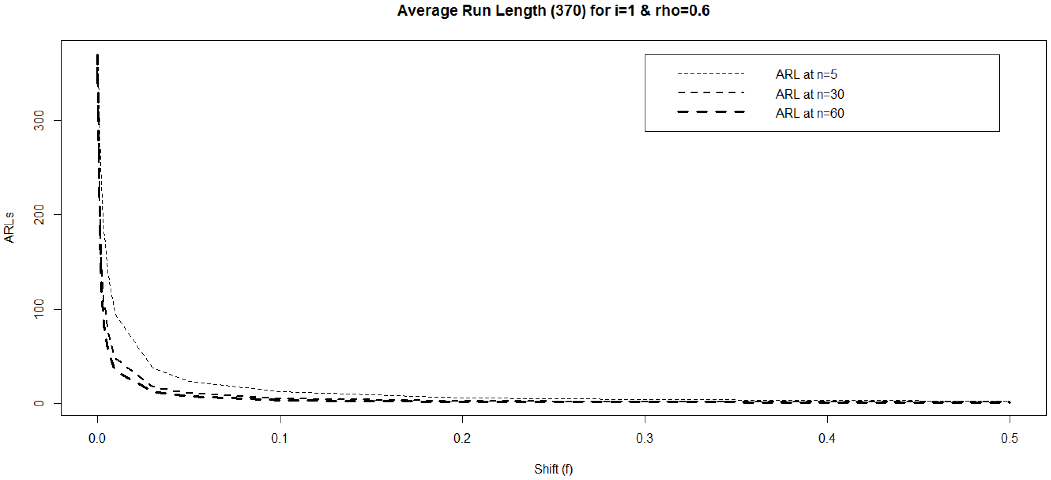
Figure 1 shows the
ARLs according to the shift constant
f for different values of
when
,
and
. It shows that
ARLs decrease faster as the sample size increases.
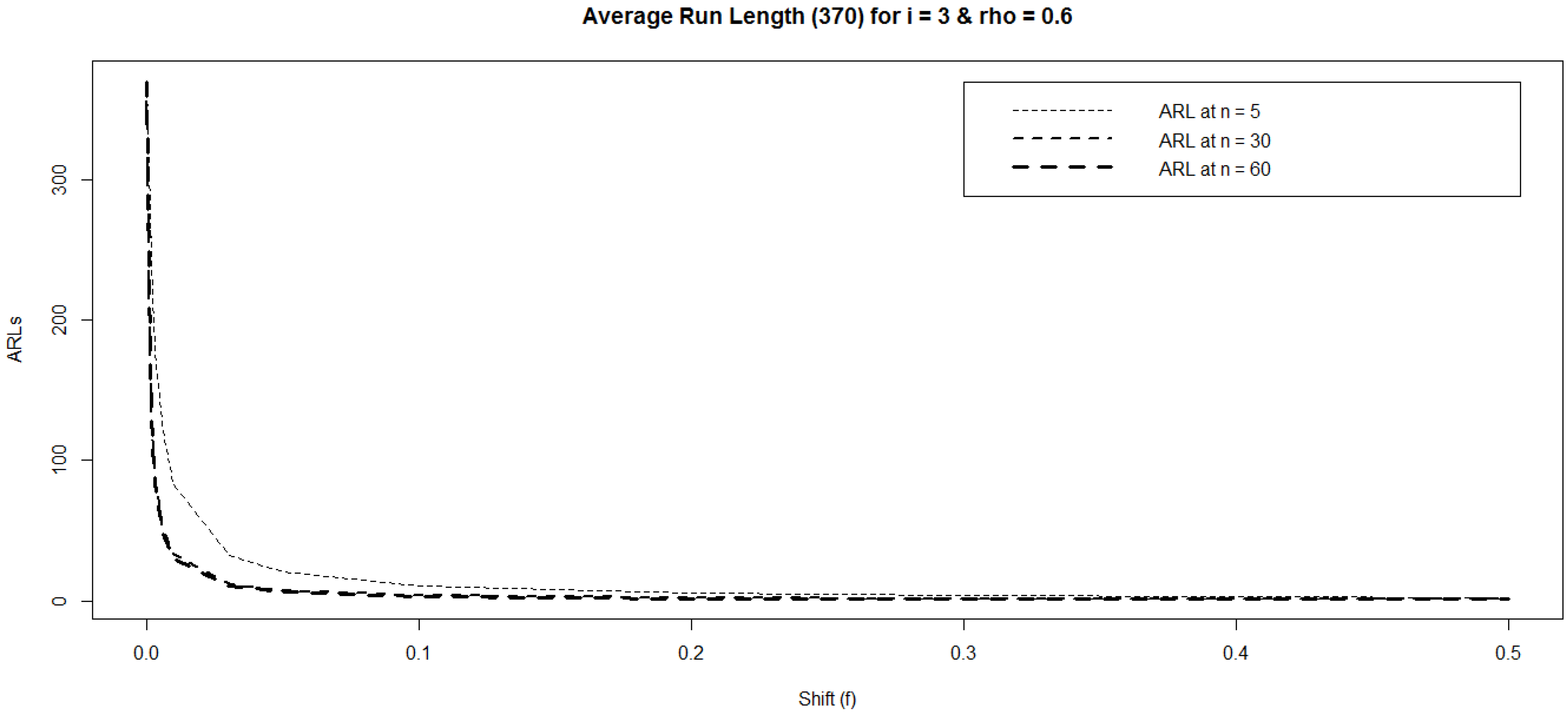
Figure 2 shows the
ARLs according to the shift constant
f for different values of
when
,
, and
. It is seen that
ARL curves may meet each other as the sample size increases. It means that the difference between
ARLs decreases as the sample size increases for higher values of
.
4. Simulation Study
In this section, we will compare the efficiency of the proposed control chart over the existing control charts using the repetitive sampling and multiple dependent state (MDS) sampling through the simulated data. The comparisons between charts will be given for the same values of control chart parameters.
The methodology of developing the proposed control chart using MDS repetitive sampling for process mean monitoring will be further explained via simulation data. In this simulation study, we consider the case of , and . A simulation data have been generated for constructing the control chart using the above mentioned parametric values. First 20 subgroups are generated from the in-control state of the process with mean zero and standard deviation 3, while the next 18 subgroups are generated from an out-of-control process with f = 0.01.
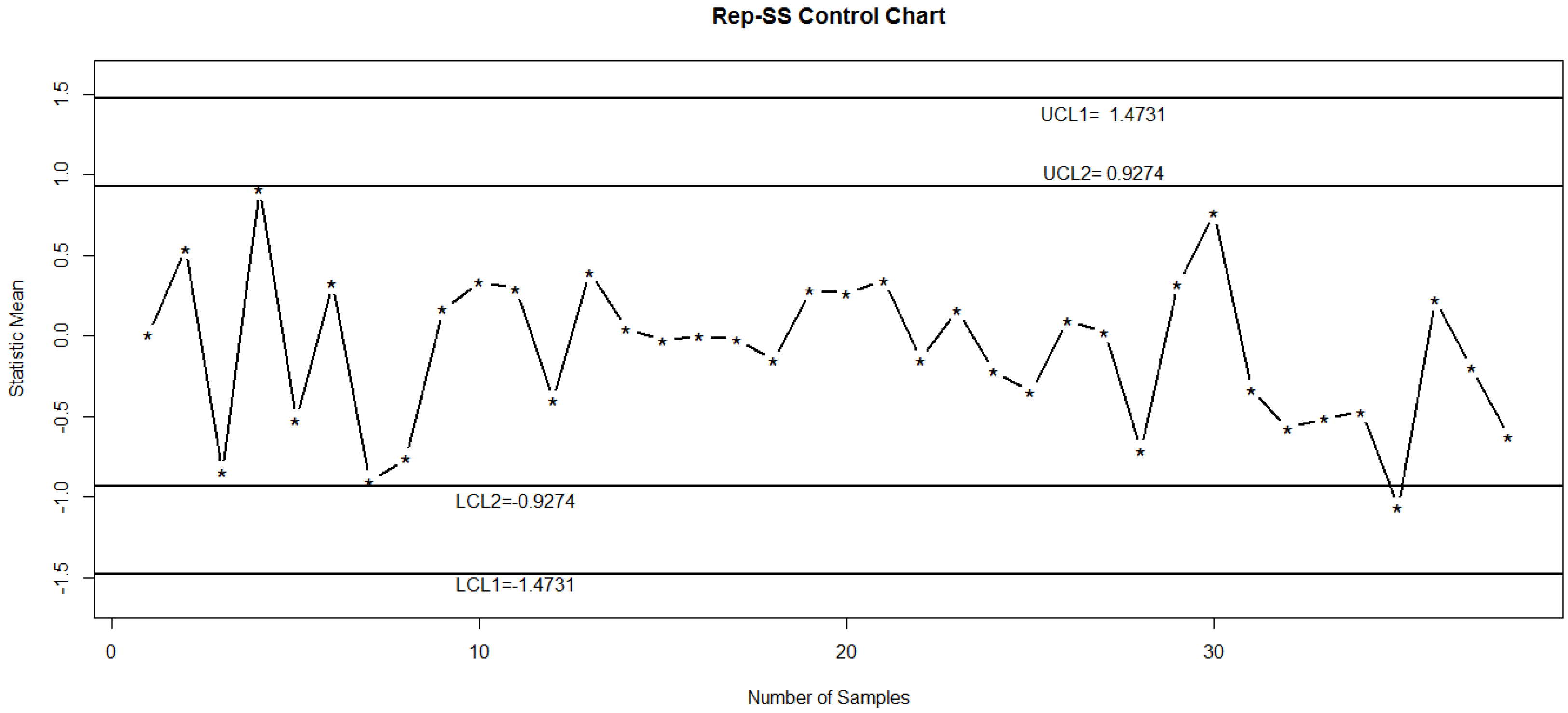
Figure 3 shows the proposed control chart, where an out-of-control signal appears at 38th subgroup. The same data is also plotted on an control chart using repetitive sampling in
Figure 4. From
Figure 4, it is noted that all points lie between
LCL1 and
UCL1, which cannot detect a shift in the process. The
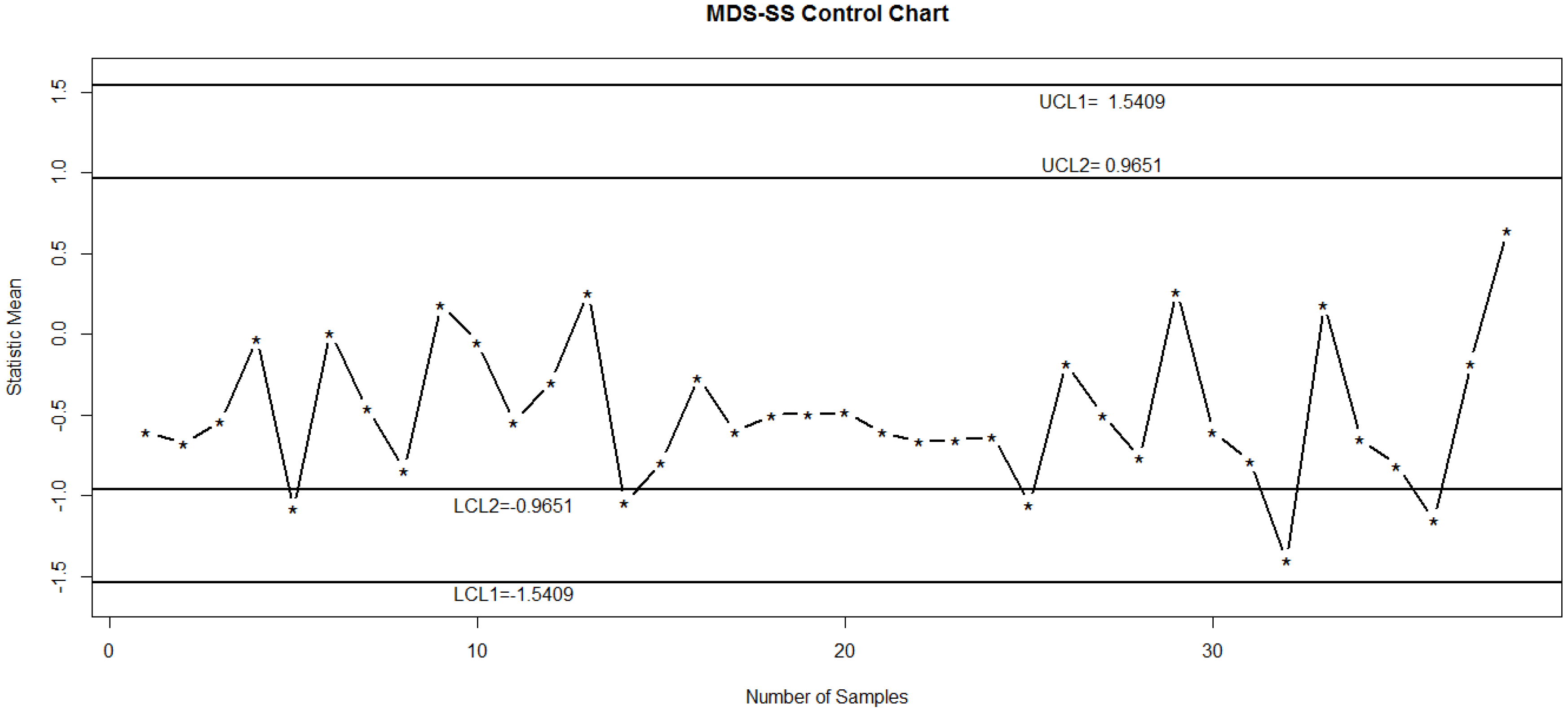
Figure 5 shows the control chart based on the MDS sampling. The control statistics are also plotted on this chart, which again cannot detect a shift in the process. So, by comparing the proposed chart with existing charts, it can be seen that the proposed chart has ability to detect a shift in the process as compared to other charts.
5. Comparison of Proposed Chart with Existing Charts
In this section, we compare the performance of the proposed chart with some existing charts including Shewhart control chart, repetitive sampling control chart, and the multiple dependent state sampling control chart using successive sampling.
Table 7,
Table 8 and
Table 9 have been prepared for
when
ARL0 = 300,
n = 5. The control chart coefficients were given. The
ARL values of the existing charts and the proposed chart for different shift levels
have been estimated and given in
Table 7,
Table 8 and
Table 9.
It can be found from these tables that the proposed chart is much faster in detecting an out-of-control process. For instance, if a process faces a shift of 0.30 then the Shewhart chart will indicate the out-of-control process after an average of 83.83 samples, Shewhart control chart 82.19, repetitive sampling control chart 80.46 and multiple dependent state sampling chart will indicate an out-of-control process in 63.20 samples while the proposed successive sampling scheme detects the same process in only 3.38 average samples. The similar detecting ability of the proposed chart for
can be observed in
Table 7,
Table 8 and
Table 9.
6. Concluding Remarks
In this article, we presented a control chart for process mean monitoring using successive sampling over two occasions and MDS sampling. The coefficients of the proposed control charts have been estimated for the target in-control ARL. Extensive tables have been constructed for different process settings to evaluate the monitoring ability of the proposed scheme. It has been observed that the proposed chart is comparatively efficient than four other existing charts in terms of the out-of-control ARLs. The proposed chart using successive sampling works well when the subgroup size is large. The performance in terms of ARL becomes better as the subgroup size increases. It is found that the performance becomes better as this correlation gets stronger. The proposed chart will be an efficient addition in the toolkit of the quality control personnel. The proposed control chart can be only used when the quality of interest follows the normal distribution. The proposed control chart for multivariate distribution can be considered as future research.
Author Contributions
Conceptualization, M.S.A., M.A., C.-H.J., and K.K.; Methodology, M.S.A., M.A., C.-H.J., and K.K.; Software, M.S.A., M.A., C.-H.J., and K.K.; Validation, M.S.A., M.A., C.-H.J. and K.K.; Formal Analysis, M.S.A., M.A., C.-H.J., and K.K.; Writing—Original Draft Preparation, M.A. and C.-H.J.; Writing—Review and Editing, M.S.A., M.A., C.-H.J., and K.K.
Funding
This research received no external funding.
Acknowledgments
The authors are deeply thankful to the editor and the reviewers for their valuable suggestions to improve the quality of this manuscript. This article was funded by the Deanship of Scientific Research (DSR) at King Abdulaziz University, Jeddah. The author, Muhammad Aslam, therefore, acknowledge with thanks DSR technical and financial support.
Conflicts of Interest
The authors declare no conflict of interest.
References
- He, D.; Grigoryan, A.; Sigh, M. Design of double-and triple-sampling X-bar control charts using genetic algorithms. Int. J. Prod. Res. 2002, 40, 1387–1404. [Google Scholar] [CrossRef]
- Montgomery, D.C. Introduction to Statistical Quality Control, 6th ed.; John Wiley & Sons, Inc.: New York, NY, USA, 2009. [Google Scholar]
- Chandara, M.J. Statistical Quality Control; CRC Press LLC: Boca Raton, FL, USA, 2001. [Google Scholar]
- Singh, H.P.; Vishwakarma, G.K. A general procedure for estimating population mean in successive sampling. Commun. Stat. Theory Methods 2009, 38, 293–308. [Google Scholar] [CrossRef]
- Rueda, M.; Martinez, S.; Arcos, A.; Munoz, J.F. Mean estimation under successive sampling with calibration estimators. Commun. Stat. Theory Methods 2009, 38, 808–827. [Google Scholar] [CrossRef]
- Valliant, R. Finite Population Sampling and Inference A Prediction Approach; John Wiley: New York, NY, USA, 2000. [Google Scholar]
- Singh, H.P.; Tailor, R.; Singh, S.; Kim, J.M. Quantile estimation in successive sampling. J. Korean Stat. Soc. 2007, 36, 543–556. [Google Scholar]
- Rueda, M.D.M.; Muñoz, J.F.; Arcos, A. Successive sampling to estimate quantiles with P-Auxiliary Variables. Qual. Quant. 2008, 42, 427–443. [Google Scholar] [CrossRef]
- Singh, G.; Priyanka, K. Estimation of population mean at current occasion in successive sampling under a super-population model. Model Assist. Stat. Appl. 2007, 2, 189–200. [Google Scholar]
- Cochran, W.G. Sampling Techniques; John Wiley & Sons: New York, NY, USA, 2007. [Google Scholar]
- Azam, M.; Nawaz, S.; Arshad, A.; Aslam, M. Acceptance Sampling Plan Using Successive Sampling over Two Successive Occasions. J. Test. Eval. 2016, 44, 2024–2032. [Google Scholar] [CrossRef]
- Jessen, R.J. Statistical investigation of a sample survey for obtaining farm facts. Res. Bull. (Iowa Agric. Home Econ. Exp. Stn.) 1942, 26, 1. [Google Scholar]
- Azam, M.; Arshad, A.; Aslam, M.; Jun, C.-H. A Control Chart for Monitoring the Process Mean Using Successive Sampling over Two Occasions. Arab. J. Sci. Eng. 2017, 42, 2915–2926. [Google Scholar] [CrossRef]
- Sen, A. Successive sampling with two auxiliary variables. Sankhyā Indian J. Stat. Ser. B 1971, 33, 371–378. [Google Scholar]
- Li, Z.H.; Zou, C.L.; Gong, Z.; Wang, Z.J. The computation of average run length and average time to signal: An overview. J. Stat. Comput. Simul. 2014, 84, 1779–1802. [Google Scholar] [CrossRef]
- Phanyaem, S.; Areepong, Y.; Sukparungsee, S. Numerical Integration of Average Run Length of CUSUM Control Chart for ARMA Process. Int. J. Appl. Phys. Math. 2014, 4, 232–235. [Google Scholar] [CrossRef]
- Knoth, S. Accurate ARL calculation for EWMA control charts monitoring normal mean and variance simultaneously. Sequential Anal. 2007, 26, 251–263. [Google Scholar] [CrossRef]
- Aslam, M.; Rao, G.S.; Ahmad, L.; Jun, C.-H. A control chart for multivariate Poisson distribution using repetitive sampling. J. Appl. Stat. 2017, 44, 123–136. [Google Scholar] [CrossRef]
- Aslam, M.; Saghir, A.; Ahamd, L.; Jun, C.-H.; Hussain, J. A control chart for COM-Poisson distribution using a modified EWMA statistic. J. Stat. Comput. Simul. 2017, 87, 1–12. [Google Scholar] [CrossRef]
- Ahmad, L.; Rafiq, I.; Aldosari, M.S.; Aslam, M. Mixed Repetitive Sampling Plan Using EWMA. Adv. Appl. Stat. 2017, 51, 167–186. [Google Scholar] [CrossRef]
- Artes Rodriguez, E.M.; Garcia Luengo, A.V. Estimation of current population ratio in successive sampling. J. Ind. Soc. Agric. Stat. 2001, 54, 342–354. [Google Scholar]
- Rueda, M.; Muñoz, J.F.; González, S.; Arcos, A. Estimating quantiles under sampling on two occasions with arbitrary sample designs. Comput. Stat. Data Anal. 2007, 51, 6596–6613. [Google Scholar] [CrossRef]
- Kowalczyk, B. Estimation of Population Parameters Using Information from Previous Period in the Case of Overlapping Samples–Simulation Study. Metody Ilościowe w Badaniach Ekonomicznych 2013, 14, 283–292. [Google Scholar]
- Aslam, M.; Nazir, A.; Jun, C.-H. A new attribute control chart using multiple dependent state sampling. Trans. Inst. Meas. Control 2015, 37, 569–576. [Google Scholar] [CrossRef]
- Chiu, J.-E.; Kuo, T.-I. Attribute control chart for multivariate Poisson distribution. Commun. Stat. Theory Methods 2007, 37, 146–158. [Google Scholar] [CrossRef]
Figure 1.
Trend of ARLs according to shift constant when , and with .
Figure 1.
Trend of ARLs according to shift constant when , and with .
Figure 2.
Trend of ARLs according to shift constant when , and with .
Figure 2.
Trend of ARLs according to shift constant when , and with .
Figure 3.
Proposed control chart for simulation data: ARL0 = 370 for and with .
Figure 3.
Proposed control chart for simulation data: ARL0 = 370 for and with .
Figure 4.
Control chart using repetitive sampling for simulation data: ARL0 = 370 for and with .
Figure 4.
Control chart using repetitive sampling for simulation data: ARL0 = 370 for and with .
Figure 5.
Control chart using MDS sampling for simulation data: ARL0 = 370 for and with .
Figure 5.
Control chart using MDS sampling for simulation data: ARL0 = 370 for and with .
Table 1.
The average run length (ARL) analysis for 300 with n = 5.
Table 1.
The average run length (ARL) analysis for 300 with n = 5.
| | | |
|---|
| | | | | | | | | | | | | | |
|---|
| | | | | |
|---|
| 2.9523 | 2.9701 | 2.9867 | 2.9953 | 2.9607 | 2.9861 | 3.0027 | 3.0211 | 2.9552 | 2.9706 | 3.0084 | 3.0170 |
|---|
| 2.9352 | | 2.9352 | | 2.9352 |
|---|
| 1.1900 | 1.1537 | 1.1238 | 1.1316 | 1.0728 | 1.0345 | 1.0323 | 1.0030 | 1.1447 | 1.1493 | 1.0040 | 1.0214 |
|---|
| 0.0000 | 300.00 | 300.00 | 300.00 | 300.00 | 300.00 | 300.00 | 300.00 | 300.00 | 300.00 | 300.00 | 300.00 | 300.00 | 300.00 | 300.00 | 300.00 |
| 0.0005 | 263.81 | 260.44 | 257.26 | 256.54 | 300.00 | 256.78 | 251.97 | 249.60 | 245.65 | 300.00 | 256.28 | 254.58 | 242.48 | 241.99 | 300.00 |
| 0.0010 | 235.41 | 230.11 | 225.20 | 224.10 | 299.99 | 224.44 | 217.21 | 213.73 | 208.01 | 299.99 | 223.69 | 221.12 | 203.50 | 202.82 | 299.99 |
| 0.0015 | 212.53 | 206.11 | 200.25 | 198.96 | 299.98 | 199.35 | 190.89 | 186.89 | 180.40 | 299.98 | 198.46 | 195.44 | 175.34 | 174.59 | 299.98 |
| 0.0020 | 193.71 | 186.65 | 180.29 | 178.91 | 299.97 | 179.31 | 170.27 | 166.05 | 159.28 | 299.97 | 178.34 | 175.11 | 154.04 | 153.28 | 299.96 |
| 0.0025 | 177.95 | 170.56 | 163.96 | 162.53 | 299.95 | 162.93 | 153.68 | 149.41 | 142.60 | 299.95 | 161.93 | 158.62 | 137.37 | 136.63 | 299.94 |
| 0.0030 | 164.57 | 157.02 | 150.35 | 148.92 | 299.93 | 149.29 | 140.04 | 135.81 | 129.10 | 299.93 | 148.29 | 144.97 | 123.97 | 123.25 | 299.91 |
| 0.0035 | 153.06 | 145.48 | 138.83 | 137.41 | 299.91 | 137.77 | 128.63 | 124.49 | 117.94 | 299.90 | 136.77 | 133.49 | 112.96 | 112.27 | 299.88 |
| 0.0040 | 143.05 | 135.52 | 128.96 | 127.56 | 299.88 | 127.90 | 118.95 | 114.91 | 108.57 | 299.87 | 126.91 | 123.70 | 103.76 | 103.09 | 299.84 |
| 0.0050 | 126.51 | 119.21 | 112.91 | 111.58 | 299.82 | 111.87 | 103.39 | 99.61 | 93.70 | 299.80 | 110.93 | 107.88 | 89.24 | 88.63 | 299.75 |
| 0.0060 | 113.41 | 106.41 | 100.42 | 99.18 | 299.74 | 99.42 | 91.45 | 87.92 | 82.43 | 299.72 | 98.52 | 95.66 | 78.30 | 77.75 | 299.65 |
| 0.0070 | 102.76 | 96.10 | 90.44 | 89.27 | 299.64 | 89.47 | 81.99 | 78.70 | 73.60 | 299.61 | 88.62 | 85.93 | 69.76 | 69.27 | 299.52 |
| 0.0080 | 93.95 | 87.62 | 82.26 | 81.16 | 299.54 | 81.33 | 74.31 | 71.24 | 66.49 | 299.50 | 80.52 | 78.00 | 62.92 | 62.46 | 299.37 |
| 0.0090 | 86.52 | 80.51 | 75.45 | 74.42 | 299.41 | 74.55 | 67.95 | 65.08 | 60.65 | 299.36 | 73.78 | 71.42 | 57.31 | 56.89 | 299.20 |
| 0.0100 | 80.19 | 74.48 | 69.69 | 68.72 | 299.28 | 68.82 | 62.60 | 59.91 | 55.76 | 299.21 | 68.09 | 65.87 | 52.62 | 52.24 | 299.02 |
| 0.0300 | 32.58 | 29.92 | 27.75 | 27.35 | 293.59 | 27.18 | 24.47 | 23.35 | 21.61 | 293.05 | 26.81 | 25.89 | 20.20 | 20.09 | 291.34 |
| 0.0500 | 20.46 | 18.79 | 17.44 | 17.21 | 282.78 | 16.98 | 15.31 | 14.65 | 13.58 | 281.39 | 16.72 | 16.18 | 12.65 | 12.61 | 277.00 |
| 0.1000 | 10.60 | 9.79 | 9.14 | 9.06 | 240.41 | 8.80 | 8.01 | 7.72 | 7.22 | 236.29 | 8.63 | 8.40 | 6.68 | 6.69 | 223.85 |
| 0.2000 | 5.38 | 5.03 | 4.76 | 4.75 | 145.54 | 4.50 | 4.18 | 4.08 | 3.87 | 138.84 | 4.37 | 4.31 | 3.55 | 3.58 | 120.48 |
| 0.3000 | 3.57 | 3.38 | 3.24 | 3.24 | 82.17 | 3.03 | 2.86 | 2.82 | 2.71 | 76.50 | 2.92 | 2.89 | 2.47 | 2.50 | 61.98 |
| 0.4000 | 2.66 | 2.55 | 2.46 | 2.47 | 47.11 | 2.30 | 2.19 | 2.18 | 2.11 | 43.07 | 2.19 | 2.18 | 1.93 | 1.95 | 33.21 |
| 0.5000 | 2.12 | 2.05 | 1.99 | 2.00 | 28.06 | 1.86 | 1.80 | 1.79 | 1.75 | 25.31 | 1.76 | 1.76 | 1.60 | 1.61 | 18.84 |
Table 2.
The ARL analysis for 300 with n = 30.
Table 2.
The ARL analysis for 300 with n = 30.
| | | |
|---|
| | | | | | | | | | | | | | |
|---|
| | | | | |
|---|
| 2.9623 | 2.9825 | 3.0048 | 3.0208 | 2.9567 | 2.9757 | 3.0031 | 3.0115 | 2.9596 | 2.9774 | 2.9905 | 3.0179 |
|---|
| 2.9352 | | 2.9352 | | 2.9352 |
|---|
| 1.0556 | 1.0581 | 1.0223 | 1.0047 | 1.1244 | 1.1075 | 1.0309 | 1.0475 | 1.0874 | 1.0945 | 1.1003 | 1.0174 |
|---|
| 0.0000 | 300.00 | 300.00 | 300.00 | 300.00 | 300.00 | 300.00 | 300.00 | 300.00 | 300.00 | 300.00 | 300.00 | 300.00 | 300.00 | 300.00 | 300.00 |
| 0.0010 | 213.49 | 209.53 | 202.35 | 197.59 | 299.99 | 216.78 | 211.79 | 200.61 | 199.93 | 299.99 | 206.55 | 203.28 | 200.87 | 188.58 | 299.99 |
| 0.0015 | 165.73 | 161.03 | 152.74 | 147.40 | 299.96 | 169.72 | 163.71 | 150.76 | 150.01 | 299.95 | 157.52 | 153.77 | 151.05 | 137.61 | 299.94 |
| 0.0020 | 135.45 | 130.79 | 122.71 | 117.60 | 299.90 | 139.46 | 133.45 | 120.80 | 120.09 | 299.89 | 127.31 | 123.68 | 121.07 | 108.40 | 299.87 |
| 0.0025 | 114.53 | 110.13 | 102.58 | 97.87 | 299.83 | 118.36 | 112.65 | 100.81 | 100.16 | 299.81 | 106.83 | 103.46 | 101.05 | 89.46 | 299.76 |
| 0.0030 | 99.22 | 95.13 | 88.15 | 83.84 | 299.73 | 102.82 | 97.47 | 86.52 | 85.94 | 299.71 | 92.04 | 88.94 | 86.74 | 76.19 | 299.63 |
| 0.0035 | 87.53 | 83.73 | 77.29 | 73.34 | 299.61 | 90.88 | 85.91 | 75.79 | 75.27 | 299.58 | 80.85 | 78.01 | 75.99 | 66.37 | 299.47 |
| 0.0040 | 78.30 | 74.78 | 68.83 | 65.20 | 299.47 | 81.44 | 76.80 | 67.45 | 66.97 | 299.42 | 72.09 | 69.47 | 67.62 | 58.81 | 299.28 |
| 0.0045 | 70.84 | 67.57 | 62.06 | 58.70 | 299.30 | 73.77 | 69.45 | 60.77 | 60.34 | 299.25 | 65.05 | 62.63 | 60.93 | 52.81 | 299.05 |
| 0.0050 | 59.51 | 56.66 | 51.87 | 48.98 | 298.91 | 62.09 | 58.31 | 50.75 | 50.38 | 298.82 | 54.42 | 52.34 | 50.88 | 43.89 | 298.53 |
| 0.0060 | 51.31 | 48.80 | 44.58 | 42.04 | 298.44 | 53.61 | 50.26 | 43.59 | 43.28 | 298.31 | 46.79 | 44.97 | 43.69 | 37.57 | 297.88 |
| 0.0070 | 45.10 | 42.87 | 39.10 | 36.85 | 297.88 | 47.17 | 44.17 | 38.22 | 37.95 | 297.70 | 41.04 | 39.43 | 38.30 | 32.87 | 297.12 |
| 0.0080 | 40.24 | 38.23 | 34.83 | 32.81 | 297.23 | 42.11 | 39.41 | 34.04 | 33.80 | 297.00 | 36.55 | 35.11 | 34.10 | 29.23 | 296.25 |
| 0.0090 | 36.32 | 34.50 | 31.42 | 29.59 | 296.51 | 38.04 | 35.58 | 30.69 | 30.48 | 296.21 | 32.95 | 31.65 | 30.75 | 26.33 | 295.27 |
| 0.0100 | 33.11 | 31.44 | 28.62 | 26.95 | 295.70 | 34.69 | 32.43 | 27.95 | 27.77 | 295.34 | 30.00 | 28.82 | 28.00 | 23.96 | 294.18 |
| 0.0300 | 12.01 | 11.48 | 10.51 | 9.94 | 264.92 | 12.60 | 11.83 | 10.24 | 10.22 | 262.26 | 10.80 | 10.45 | 10.21 | 8.81 | 254.02 |
| 0.0500 | 7.37 | 7.10 | 6.56 | 6.25 | 218.00 | 7.71 | 7.29 | 6.39 | 6.40 | 212.83 | 6.60 | 6.44 | 6.33 | 5.54 | 197.59 |
| 0.1000 | 3.77 | 3.69 | 3.48 | 3.36 | 112.69 | 3.91 | 3.76 | 3.38 | 3.41 | 106.24 | 3.36 | 3.32 | 3.30 | 2.98 | 89.15 |
| 0.2000 | 1.94 | 1.93 | 1.87 | 1.84 | 29.51 | 1.97 | 1.94 | 1.82 | 1.84 | 26.65 | 1.73 | 1.73 | 1.73 | 1.64 | 19.89 |
| 0.3000 | 1.37 | 1.37 | 1.35 | 1.34 | 9.85 | 1.37 | 1.36 | 1.32 | 1.33 | 8.74 | 1.24 | 1.25 | 1.25 | 1.22 | 6.26 |
| 0.4000 | 1.14 | 1.14 | 1.13 | 1.13 | 4.23 | 1.13 | 1.13 | 1.11 | 1.12 | 3.76 | 1.07 | 1.07 | 1.07 | 1.06 | 2.75 |
| 0.5000 | 1.05 | 1.05 | 1.04 | 1.04 | 2.30 | 1.04 | 1.04 | 1.03 | 1.03 | 2.08 | 1.02 | 1.02 | 1.02 | 1.01 | 1.62 |
Table 3.
The ARL analysis for 300 with n = 60.
Table 3.
The ARL analysis for 300 with n = 60.
| | | |
|---|
| | | | | | | | | | | | | | |
|---|
| | | | | |
|---|
| 2.9590 | 2.9752 | 2.9953 | 3.0033 | 2.9574 | 2.9849 | 3.0039 | 3.0150 | 2.9618 | 2.9804 | 2.9915 | 2.9984 |
|---|
| 2.9352 | | 2.9352 | | 2.9352 |
|---|
| 1.0940 | 1.1113 | 1.0727 | 1.0884 | 1.1152 | 1.0424 | 1.0264 | 1.0307 | 1.0612 | 1.0727 | 1.0948 | 1.1143 |
|---|
| 0.0000 | 300.00 | 300.00 | 300.00 | 300.00 | 300.00 | 300.00 | 300.00 | 300.00 | 300.00 | 300.00 | 300.00 | 300.00 | 300.00 | 300.00 | 300.00 |
| 0.0005 | 194.36 | 192.08 | 184.45 | 183.81 | 299.98 | 193.57 | 181.61 | 175.88 | 173.54 | 299.98 | 180.38 | 176.89 | 176.05 | 175.99 | 299.97 |
| 0.0010 | 143.77 | 141.32 | 133.25 | 132.60 | 299.91 | 142.90 | 130.29 | 124.51 | 122.20 | 299.91 | 128.99 | 125.49 | 124.67 | 124.62 | 299.88 |
| 0.0015 | 114.09 | 111.81 | 104.35 | 103.77 | 299.80 | 113.28 | 101.63 | 96.43 | 94.38 | 299.79 | 100.41 | 97.28 | 96.56 | 96.53 | 299.73 |
| 0.0020 | 94.58 | 92.52 | 85.79 | 85.28 | 299.65 | 93.83 | 83.33 | 78.72 | 76.92 | 299.62 | 82.21 | 79.45 | 78.83 | 78.82 | 299.53 |
| 0.0025 | 80.78 | 78.92 | 72.86 | 72.41 | 299.46 | 80.09 | 70.64 | 66.54 | 64.95 | 299.41 | 69.61 | 67.16 | 66.63 | 66.63 | 299.26 |
| 0.0030 | 70.50 | 68.82 | 63.33 | 62.94 | 299.22 | 69.87 | 61.31 | 57.64 | 56.23 | 299.15 | 60.36 | 58.18 | 57.71 | 57.72 | 298.94 |
| 0.0035 | 62.54 | 61.02 | 56.02 | 55.67 | 298.94 | 61.96 | 54.17 | 50.86 | 49.59 | 298.85 | 53.29 | 51.33 | 50.92 | 50.93 | 298.55 |
| 0.0040 | 56.20 | 54.82 | 50.24 | 49.92 | 298.61 | 55.67 | 48.53 | 45.51 | 44.37 | 298.49 | 47.71 | 45.93 | 45.57 | 45.59 | 298.11 |
| 0.0050 | 46.74 | 45.57 | 41.66 | 41.41 | 297.84 | 46.28 | 40.19 | 37.64 | 36.68 | 297.65 | 39.45 | 37.96 | 37.67 | 37.70 | 297.06 |
| 0.0060 | 40.01 | 39.00 | 35.61 | 35.40 | 296.89 | 39.60 | 34.31 | 32.11 | 31.29 | 296.63 | 33.63 | 32.37 | 32.13 | 32.17 | 295.78 |
| 0.0070 | 34.98 | 34.10 | 31.11 | 30.93 | 295.78 | 34.61 | 29.94 | 28.02 | 27.30 | 295.43 | 29.32 | 28.22 | 28.02 | 28.07 | 294.29 |
| 0.0080 | 31.07 | 30.30 | 27.63 | 27.48 | 294.51 | 30.74 | 26.57 | 24.86 | 24.23 | 294.05 | 25.99 | 25.03 | 24.86 | 24.91 | 292.58 |
| 0.0090 | 27.96 | 27.27 | 24.86 | 24.73 | 293.09 | 27.66 | 23.89 | 22.36 | 21.80 | 292.51 | 23.35 | 22.49 | 22.35 | 22.40 | 290.66 |
| 0.0100 | 25.41 | 24.80 | 22.60 | 22.49 | 291.51 | 25.13 | 21.71 | 20.32 | 19.82 | 290.80 | 21.19 | 20.42 | 20.30 | 20.36 | 288.55 |
| 0.0300 | 9.05 | 8.91 | 8.20 | 8.21 | 236.55 | 8.93 | 7.81 | 7.39 | 7.26 | 232.24 | 7.50 | 7.31 | 7.33 | 7.39 | 219.25 |
| 0.0500 | 5.52 | 5.47 | 5.09 | 5.12 | 168.68 | 5.44 | 4.83 | 4.62 | 4.57 | 162.16 | 4.58 | 4.50 | 4.54 | 4.60 | 143.87 |
| 0.1000 | 2.80 | 2.81 | 2.68 | 2.70 | 63.22 | 2.75 | 2.52 | 2.46 | 2.46 | 58.32 | 2.34 | 2.34 | 2.37 | 2.41 | 46.09 |
| 0.2000 | 1.47 | 1.48 | 1.45 | 1.46 | 11.67 | 1.43 | 1.38 | 1.37 | 1.37 | 10.37 | 1.28 | 1.29 | 1.30 | 1.31 | 7.45 |
| 0.3000 | 1.12 | 1.12 | 1.11 | 1.11 | 3.58 | 1.10 | 1.09 | 1.08 | 1.08 | 3.19 | 1.05 | 1.05 | 1.05 | 1.05 | 2.36 |
| 0.4000 | 1.02 | 1.02 | 1.02 | 1.02 | 1.73 | 1.02 | 1.01 | 1.01 | 1.01 | 1.59 | 1.00 | 1.00 | 1.01 | 1.01 | 1.31 |
| 0.5000 | 1.00 | 1.00 | 1.00 | 1.00 | 1.19 | 1.00 | 1.00 | 1.00 | 1.00 | 1.14 | 1.00 | 1.00 | 1.00 | 1.00 | 1.05 |
Table 4.
The ARL analysis for 370 with n = 5.
Table 4.
The ARL analysis for 370 with n = 5.
| | | |
|---|
| | | | | | | | | | | | | | |
|---|
| | | | | |
|---|
| 3.0175 | 3.0326 | 3.0469 | 3.0759 | 3.0104 | 3.0210 | 3.0335 | 3.0694 | 3.0087 | 3.0278 | 3.0586 | 3.0706 |
|---|
| 2.9997 | | 2.9997 | | 2.9997 |
|---|
| 1.1753 | 1.1665 | 1.1469 | 1.0418 | 1.3191 | 1.2952 | 1.2528 | 1.0740 | 1.3652 | 1.2146 | 1.0737 | 1.0678 |
|---|
| 0.0000 | 370.00 | 370.00 | 370.00 | 370.00 | 370.00 | 370.00 | 370.00 | 370.00 | 370.00 | 370.00 | 370.00 | 370.00 | 370.00 | 370.00 | 370.00 |
| 0.0005 | 315.26 | 312.36 | 308.82 | 297.06 | 370.00 | 322.58 | 319.72 | 315.36 | 297.97 | 370.00 | 320.73 | 308.39 | 293.40 | 290.51 | 370.00 |
| 0.0010 | 274.63 | 270.26 | 265.02 | 248.18 | 369.99 | 285.93 | 281.47 | 274.79 | 249.45 | 369.99 | 283.05 | 264.39 | 243.11 | 239.18 | 369.99 |
| 0.0015 | 243.29 | 238.18 | 232.12 | 213.15 | 369.98 | 256.76 | 251.41 | 243.49 | 214.54 | 369.98 | 253.29 | 231.38 | 207.57 | 203.30 | 369.97 |
| 0.0020 | 218.37 | 212.91 | 206.49 | 186.80 | 369.96 | 233.00 | 227.15 | 218.59 | 188.23 | 369.96 | 229.19 | 205.71 | 181.11 | 176.80 | 369.95 |
| 0.0025 | 198.08 | 192.50 | 185.97 | 166.27 | 369.94 | 213.26 | 207.16 | 198.32 | 167.68 | 369.94 | 209.28 | 185.17 | 160.65 | 156.43 | 369.92 |
| 0.0030 | 181.24 | 175.66 | 169.17 | 149.81 | 369.92 | 196.60 | 190.41 | 181.50 | 151.19 | 369.91 | 192.55 | 168.37 | 144.35 | 140.28 | 369.89 |
| 0.0035 | 167.05 | 161.54 | 155.16 | 136.34 | 369.89 | 182.36 | 176.17 | 167.31 | 137.66 | 369.88 | 178.30 | 154.36 | 131.07 | 127.17 | 369.84 |
| 0.0040 | 154.92 | 149.52 | 143.30 | 125.09 | 369.85 | 170.04 | 163.91 | 155.18 | 126.37 | 369.84 | 166.02 | 142.51 | 120.03 | 116.31 | 369.80 |
| 0.0050 | 135.27 | 130.16 | 124.31 | 107.40 | 369.77 | 149.81 | 143.90 | 135.55 | 108.57 | 369.75 | 145.91 | 123.55 | 102.74 | 99.36 | 369.68 |
| 0.0060 | 120.05 | 115.25 | 109.78 | 94.12 | 369.66 | 133.88 | 128.24 | 120.33 | 95.19 | 369.64 | 130.14 | 109.05 | 89.83 | 86.75 | 369.54 |
| 0.0070 | 107.91 | 103.41 | 98.30 | 83.77 | 369.54 | 121.01 | 115.66 | 108.20 | 84.76 | 369.50 | 117.45 | 97.61 | 79.81 | 76.99 | 369.38 |
| 0.0080 | 98.01 | 93.79 | 89.00 | 75.49 | 369.40 | 110.40 | 105.33 | 98.29 | 76.41 | 369.35 | 107.02 | 88.34 | 71.82 | 69.22 | 369.19 |
| 0.0090 | 89.77 | 85.80 | 81.32 | 68.71 | 369.25 | 101.50 | 96.70 | 90.05 | 69.56 | 369.18 | 98.29 | 80.68 | 65.29 | 62.89 | 368.97 |
| 0.0100 | 82.81 | 79.08 | 74.86 | 63.06 | 369.07 | 93.93 | 89.38 | 83.09 | 63.85 | 368.99 | 90.87 | 74.25 | 59.85 | 57.63 | 368.74 |
| 0.0300 | 32.52 | 30.91 | 29.11 | 24.10 | 361.78 | 37.70 | 35.61 | 32.77 | 24.42 | 361.09 | 36.21 | 28.72 | 22.67 | 21.81 | 358.89 |
| 0.0500 | 20.26 | 19.28 | 18.18 | 15.07 | 347.94 | 23.57 | 22.27 | 20.49 | 15.26 | 346.16 | 22.58 | 17.86 | 14.12 | 13.61 | 340.55 |
| 0.1000 | 10.44 | 9.99 | 9.48 | 7.95 | 294.01 | 12.13 | 11.50 | 10.63 | 8.03 | 288.80 | 11.57 | 9.21 | 7.38 | 7.17 | 273.09 |
| 0.2000 | 5.28 | 5.11 | 4.90 | 4.22 | 175.21 | 6.06 | 5.80 | 5.42 | 4.24 | 166.93 | 5.72 | 4.67 | 3.87 | 3.79 | 144.30 |
| 0.3000 | 3.52 | 3.43 | 3.32 | 2.93 | 97.46 | 3.96 | 3.82 | 3.61 | 2.93 | 90.57 | 3.70 | 3.10 | 2.65 | 2.62 | 73.00 |
| 0.4000 | 2.63 | 2.58 | 2.52 | 2.27 | 55.12 | 2.90 | 2.82 | 2.69 | 2.25 | 50.28 | 2.68 | 2.31 | 2.04 | 2.02 | 38.51 |
| 0.5000 | 2.10 | 2.07 | 2.03 | 1.87 | 32.40 | 2.27 | 2.22 | 2.13 | 1.84 | 29.15 | 2.08 | 1.85 | 1.67 | 1.66 | 21.52 |
Table 5.
The ARL analysis for 370 with n = 30.
Table 5.
The ARL analysis for 370 with n = 30.
| | | |
|---|
| | | | | | | | | | | | | | |
|---|
| | | | | |
|---|
| 3.0131 | 3.0248 | 3.0473 | 3.0559 | 3.0088 | 3.0276 | 3.0482 | 3.0714 | 3.0124 | 3.0318 | 3.0509 | 3.0801 |
|---|
| 2.9997 | | 2.9997 | | 2.9997 |
|---|
| 1.2566 | 1.2484 | 1.1445 | 1.1498 | 1.3626 | 1.2171 | 1.1381 | 1.0641 | 1.2719 | 1.1746 | 1.1203 | 1.0221 |
|---|
| 0.0000 | 370.00 | 370.00 | 370.00 | 370.00 | 370.00 | 370.00 | 370.00 | 370.00 | 370.00 | 370.00 | 370.00 | 370.00 | 370.00 | 370.00 | 370.00 |
| 0.0005 | 268.36 | 264.68 | 248.82 | 246.99 | 369.99 | 276.66 | 257.79 | 244.58 | 230.95 | 369.98 | 258.36 | 243.33 | 232.51 | 214.40 | 369.98 |
| 0.0010 | 210.53 | 206.06 | 187.50 | 185.44 | 369.94 | 220.93 | 197.83 | 182.73 | 167.96 | 369.94 | 198.49 | 181.32 | 169.59 | 151.05 | 369.92 |
| 0.0015 | 173.22 | 168.72 | 150.46 | 148.49 | 369.87 | 183.89 | 160.53 | 145.89 | 132.04 | 369.86 | 161.15 | 144.52 | 133.52 | 116.68 | 369.83 |
| 0.0020 | 147.14 | 142.85 | 125.67 | 123.86 | 369.78 | 157.49 | 135.07 | 121.44 | 108.81 | 369.76 | 135.64 | 120.16 | 110.14 | 95.10 | 369.70 |
| 0.0025 | 127.89 | 123.86 | 107.92 | 106.26 | 369.65 | 137.72 | 116.60 | 104.03 | 92.57 | 369.62 | 117.10 | 102.84 | 93.75 | 80.29 | 369.52 |
| 0.0030 | 113.10 | 109.34 | 94.57 | 93.06 | 369.50 | 122.36 | 102.57 | 91.00 | 80.56 | 369.45 | 103.03 | 89.89 | 81.62 | 69.49 | 369.32 |
| 0.0035 | 101.38 | 97.87 | 84.18 | 82.79 | 369.32 | 110.08 | 91.57 | 80.89 | 71.33 | 369.26 | 91.97 | 79.85 | 72.28 | 61.28 | 369.07 |
| 0.0040 | 91.86 | 88.58 | 75.85 | 74.57 | 369.11 | 100.04 | 82.70 | 72.81 | 64.02 | 369.03 | 83.06 | 71.83 | 64.88 | 54.82 | 368.79 |
| 0.0050 | 77.34 | 74.46 | 63.34 | 62.24 | 368.61 | 84.61 | 69.30 | 60.70 | 53.15 | 368.49 | 69.59 | 59.83 | 53.86 | 45.30 | 368.11 |
| 0.0060 | 66.78 | 64.24 | 54.39 | 53.44 | 368.00 | 73.30 | 59.64 | 52.06 | 45.46 | 367.83 | 59.87 | 51.28 | 46.06 | 38.63 | 367.28 |
| 0.0070 | 58.77 | 56.48 | 47.67 | 46.83 | 367.28 | 64.66 | 52.35 | 45.60 | 39.74 | 367.05 | 52.54 | 44.88 | 40.25 | 33.69 | 366.30 |
| 0.0080 | 52.47 | 50.41 | 42.44 | 41.69 | 366.45 | 57.84 | 46.66 | 40.57 | 35.31 | 366.15 | 46.81 | 39.90 | 35.76 | 29.89 | 365.19 |
| 0.0090 | 47.39 | 45.52 | 38.26 | 37.58 | 365.52 | 52.32 | 42.09 | 36.55 | 31.78 | 365.14 | 42.21 | 35.92 | 32.17 | 26.87 | 363.92 |
| 0.0100 | 43.21 | 41.49 | 34.83 | 34.21 | 364.48 | 47.76 | 38.33 | 33.26 | 28.90 | 364.02 | 38.43 | 32.67 | 29.25 | 24.42 | 362.53 |
| 0.0300 | 15.63 | 15.05 | 12.63 | 12.45 | 325.15 | 17.37 | 13.85 | 12.04 | 10.52 | 321.76 | 13.76 | 11.71 | 10.54 | 8.89 | 311.28 |
| 0.0500 | 9.52 | 9.20 | 7.80 | 7.72 | 265.71 | 10.55 | 8.47 | 7.43 | 6.57 | 259.21 | 8.34 | 7.17 | 6.51 | 5.58 | 240.06 |
| 0.1000 | 4.75 | 4.63 | 4.03 | 4.01 | 134.74 | 5.19 | 4.28 | 3.84 | 3.48 | 126.83 | 4.12 | 3.64 | 3.38 | 3.00 | 105.95 |
| 0.2000 | 2.30 | 2.27 | 2.07 | 2.07 | 34.12 | 2.42 | 2.12 | 1.98 | 1.86 | 30.73 | 1.98 | 1.83 | 1.76 | 1.64 | 22.76 |
| 0.3000 | 1.52 | 1.51 | 1.43 | 1.44 | 11.04 | 1.55 | 1.43 | 1.38 | 1.33 | 9.76 | 1.34 | 1.29 | 1.26 | 1.22 | 6.92 |
| 0.4000 | 1.20 | 1.20 | 1.16 | 1.17 | 4.61 | 1.21 | 1.16 | 1.14 | 1.12 | 4.08 | 1.10 | 1.09 | 1.08 | 1.06 | 2.95 |
| 0.5000 | 1.07 | 1.07 | 1.05 | 1.06 | 2.44 | 1.07 | 1.05 | 1.04 | 1.04 | 2.20 | 1.03 | 1.02 | 1.02 | 1.01 | 1.69 |
Table 6.
The ARL analysis for 370 with .
Table 6.
The ARL analysis for 370 with .
| | | |
|---|
| | | | | | | | | | | | | | |
|---|
| k1 | k | k1 | k | k1 | k |
|---|
| 3.0161 | 3.0418 | 3.0597 | 3.0705 | 3.0093 | 3.0220 | 3.0300 | 3.0548 | 3.0218 | 3.0464 | 3.0652 | 3.0825 |
|---|
| k2 | 2.9997 | k2 | 2.9997 | k2 | 2.9997 |
|---|
| 1.1988 | 1.0905 | 1.0675 | 1.0686 | 1.3468 | 1.2827 | 1.2855 | 1.1562 | 1.1118 | 1.0569 | 1.0372 | 1.0110 |
|---|
| 0.0000 | 370.00 | 370.00 | 370.00 | 370.00 | 370.00 | 370.00 | 370.00 | 370.00 | 370.00 | 370.00 | 370.00 | 370.00 | 370.00 | 370.00 | 370.00 |
| 0.0005 | 233.92 | 215.25 | 207.54 | 204.36 | 369.97 | 248.56 | 237.87 | 235.91 | 214.44 | 369.97 | 209.48 | 196.44 | 188.70 | 180.84 | 369.96 |
| 0.0010 | 171.04 | 151.85 | 144.32 | 141.30 | 369.89 | 187.14 | 175.31 | 173.21 | 151.07 | 369.88 | 146.13 | 133.80 | 126.78 | 119.83 | 369.85 |
| 0.0015 | 134.82 | 117.34 | 110.69 | 108.05 | 369.75 | 150.06 | 138.82 | 136.87 | 116.68 | 369.73 | 112.22 | 101.50 | 95.53 | 89.69 | 369.66 |
| 0.0020 | 111.27 | 95.64 | 89.81 | 87.52 | 369.55 | 125.25 | 114.92 | 113.16 | 95.08 | 369.51 | 91.10 | 81.80 | 76.68 | 71.73 | 369.39 |
| 0.0025 | 94.72 | 80.73 | 75.59 | 73.58 | 369.30 | 107.48 | 98.05 | 96.47 | 80.26 | 369.24 | 76.68 | 68.52 | 64.08 | 59.80 | 369.05 |
| 0.0030 | 82.47 | 69.86 | 65.27 | 63.49 | 369.00 | 94.12 | 85.51 | 84.08 | 69.46 | 368.91 | 66.20 | 58.97 | 55.06 | 51.30 | 368.63 |
| 0.0035 | 73.02 | 61.58 | 57.45 | 55.86 | 368.63 | 83.72 | 75.82 | 74.51 | 61.23 | 368.52 | 58.25 | 51.77 | 48.28 | 44.94 | 368.14 |
| 0.0040 | 65.52 | 55.06 | 51.32 | 49.88 | 368.22 | 75.39 | 68.10 | 66.91 | 54.76 | 368.07 | 52.01 | 46.14 | 43.00 | 40.00 | 367.58 |
| 0.0050 | 54.36 | 45.46 | 42.31 | 41.11 | 367.22 | 62.88 | 56.59 | 55.59 | 45.23 | 366.99 | 42.84 | 37.92 | 35.31 | 32.82 | 366.23 |
| 0.0060 | 46.45 | 38.72 | 36.02 | 34.99 | 366.01 | 53.92 | 48.42 | 47.55 | 38.55 | 365.67 | 36.42 | 32.21 | 29.98 | 27.86 | 364.59 |
| 0.0070 | 40.55 | 33.74 | 31.37 | 30.48 | 364.59 | 47.20 | 42.32 | 41.56 | 33.61 | 364.13 | 31.69 | 28.00 | 26.07 | 24.22 | 362.67 |
| 0.0080 | 35.99 | 29.90 | 27.80 | 27.02 | 362.96 | 41.97 | 37.58 | 36.91 | 29.80 | 362.37 | 28.04 | 24.78 | 23.07 | 21.44 | 360.48 |
| 0.0090 | 32.35 | 26.85 | 24.97 | 24.27 | 361.13 | 37.78 | 33.80 | 33.20 | 26.78 | 360.39 | 25.15 | 22.23 | 20.70 | 19.25 | 358.03 |
| 0.0100 | 29.38 | 24.38 | 22.67 | 22.04 | 359.11 | 34.35 | 30.72 | 30.18 | 24.32 | 358.20 | 22.81 | 20.16 | 18.78 | 17.47 | 355.32 |
| 0.0300 | 10.37 | 8.68 | 8.15 | 7.99 | 289.14 | 12.13 | 10.89 | 10.74 | 8.75 | 283.68 | 7.99 | 7.17 | 6.77 | 6.38 | 267.29 |
| 0.0500 | 6.28 | 5.34 | 5.06 | 4.99 | 203.94 | 7.28 | 6.59 | 6.53 | 5.41 | 195.84 | 4.85 | 4.42 | 4.22 | 4.02 | 173.16 |
| 0.1000 | 3.12 | 2.75 | 2.66 | 2.65 | 74.50 | 3.50 | 3.24 | 3.23 | 2.79 | 68.59 | 2.45 | 2.30 | 2.25 | 2.19 | 53.89 |
| 0.2000 | 1.55 | 1.46 | 1.44 | 1.44 | 13.15 | 1.63 | 1.57 | 1.57 | 1.46 | 11.65 | 1.31 | 1.28 | 1.27 | 1.26 | 8.28 |
| 0.3000 | 1.14 | 1.12 | 1.11 | 1.11 | 3.87 | 1.16 | 1.14 | 1.14 | 1.11 | 3.44 | 1.05 | 1.05 | 1.05 | 1.04 | 2.51 |
| 0.4000 | 1.03 | 1.02 | 1.02 | 1.02 | 1.81 | 1.03 | 1.02 | 1.02 | 1.02 | 1.65 | 1.01 | 1.00 | 1.00 | 1.00 | 1.34 |
| 0.5000 | 1.00 | 1.00 | 1.00 | 1.00 | 1.22 | 1.00 | 1.00 | 1.00 | 1.00 | 1.16 | 1.00 | 1.00 | 1.00 | 1.00 | 1.06 |
Table 7.
ARL comparison when .
Table 7.
ARL comparison when .
| f | Shewhart Control Chart | Repetitive Sampling Control Chart | MDS Sampling Chart | Proposed Chart |
|---|
| |
|---|
| | | |
|---|
| | |
|---|
| 0.0 | 300.08 | 300 | 300 | 300 |
| 0.1 | 241.6 | 239.91 | 234.75 | 9.79 |
| 0.2 | 147.47 | 144.2 | 129.56 | 5.03 |
| 0.3 | 83.83 | 80.46 | 63.2 | 3.38 |
| 0.4 | 48.32 | 45.36 | 31.04 | 2.55 |
| 0.5 | 28.89 | 26.42 | 16.19 | 2.05 |
Table 8.
ARL comparison when .
Table 8.
ARL comparison when .
| f | Shewhart Control Chart | Repetitive Sampling Control Chart | MDS Sampling Chart | Proposed Chart |
|---|
| |
|---|
| | | |
|---|
| | |
|---|
| 0 | 300.08 | 300 | 300 | 300 |
| 0.1 | 241.6 | 235.76 | 230.13 | 8.01 |
| 0.2 | 147.47 | 137.45 | 122.21 | 4.18 |
| 0.3 | 83.83 | 74.77 | 57.66 | 2.86 |
| 0.4 | 48.32 | 41.33 | 27.69 | 2.19 |
| 0.5 | 28.89 | 23.71 | 14.26 | 1.8 |
Table 9.
ARL comparison when .
Table 9.
ARL comparison when .
| f | Shewhart Control Chart | Repetitive Sampling Control Chart | MDS Sampling Chart | Proposed Chart |
|---|
| |
|---|
| | | |
|---|
| | |
|---|
| 0 | 300.08 | 300 | 300 | 300 |
| 0.1 | 241.6 | 223.2 | 220.97 | 8.4 |
| 0.2 | 147.47 | 118.96 | 114.85 | 4.31 |
| 0.3 | 83.83 | 60.23 | 56.16 | 2.89 |
| 0.4 | 48.32 | 31.52 | 28.32 | 2.18 |
| 0.5 | 28.89 | 17.34 | 15.1 | 1.76 |
© 2018 by the authors. Licensee MDPI, Basel, Switzerland. This article is an open access article distributed under the terms and conditions of the Creative Commons Attribution (CC BY) license (http://creativecommons.org/licenses/by/4.0/).


