Changes in Natural Disaster Risk: Macroeconomic Responses in Selected Latin American Countries


1
HECER, University of Helsinki, FI-00014 Helsinki, Finland
2
Bank of Finland, 00101 Helsinki, Finland1
Economies 2018, 6(1), 13; https://doi.org/10.3390/economies6010013
Submission received: 29 November 2017
/
Revised: 31 January 2018
/
Accepted: 1 February 2018
/
Published: 26 February 2018
(This article belongs to the Special Issue Natural Hazards and Economic Development)
Abstract
:This paper studies the theoretical effects of changes in disaster risk on macroeconomic variables in five Latin American economies. It compares country-specific variants of the New Keynesian model with disaster risk developed by Isoré and Szczerbowicz (2017). Countries with higher price flexibility, such as Argentina, Brazil, and Mexico, are found to be relatively less vulnerable to disaster risk shocks, as compared to Chile and Colombia in particular. Overall, the analysis suggests that increases in the probability of natural disasters over time may have significant macroeconomic effects, beyond the direct impact of actual disaster occurrences themselves.
JEL Classification:
E20; E31; E32; Q541. Introduction
Evidence regarding the macroeconomic effects of natural disasters is scarce and not yet conclusive. In particular, it seems that natural events need to be “extreme” to significantly impact a country’s short or long term GDP growth (Cavallo et al. 2013). The most commonly used database of natural disasters, EM-DAT (www.emdat.be) includes a very large range of situations that “overwhelms local capacity and/or necessitates a request for external assistance”, from floods to earthquakes among many others. Yet, what may look like a catastrophe at the local level does not necessarily matter at aggregate levels, unless the geographical size of the country is itself very small, such as Haiti, for instance (Cavallo et al. 2010). Therefore, while negative effects are found on specific samples or disaster types (e.g., Hsiang and Jina (2014) for cyclones), no significant impact emerge in meta-analyses of indirect costs (Lazzaroni and van Bergeijk 2014).2 Skidmore and Toya (2002) even argue that natural disasters may even have a positive long run growth effect via the reconstruction activities in the recovery phase. From a theoretical point of view, the impact of disasters on growth is also ambiguous. Standard growth model would predict that a sudden destruction of the physical capital stock increases output growth by stimulating savings and investment. On the contrary, endogenous growth models with increasing returns to scale may find negative effects. Hence, the consequences of actual natural disasters on dynamic macroeconomic variables are far from clear-cut, both theoretically and empirically.
Meanwhile, a recent but growing macroeconomic literature has emphasized the role of disaster risk on economic outcomes, starting with the seminal paper by Barro (2006). Originally designed for replicating asset pricing features, such as the risk premium puzzle, this literature has been further developed into dynamic and stochastic macroeconomic models. Gabaix (2011), Gabaix (2012), and Gourio (2012) have introduced a small but time-varying probability of disasters in real business cycle models, and find that changes in the probability of disasters, without any arrival of the disaster itself, may suffice to trigger economic recessions. Isoré and Szczerbowicz (2017) further showed how to extend this approach to a New Keynesian environment, and found that disaster risk shocksn—again, absent of actual disaster realization—, generate procyclical responses of consumption, investment, labor, wage, and inflation, simultaneously to the recession and rise in equity premium. Further empirical evidence by Siriwardane (2015) and Marfè and Penasse (2017) support the relationship between changes in the probability of a disaster and macroeconomic variables.
It may seem like a paradox that changes in disaster risk affect real macroeconomic variables when natural disasters themselves generally do not. The disaster risk literature defines “disasters” as rare events destroying a large share of a country’s existing capital stock. Even though it often focuses on political or financial disasters, it also encompasses extreme natural events, by definition. Therefore, this suggests that it is not so much the arrival of actual natural disasters that affects the dynamic paths of macroeconomic variables, but the simple risk that they may occur, i.e the uncertainty component that is embedded in changes in their probability over time.
In this paper, changes in disaster risk are simulated for five Latin American countries—namely Argentina, Brazil, Chile, Colombia, and Mexico—using variants from the New Keynesian DSGE model developed by Isoré and Szczerbowicz (2017). This study is the first analysis of the effects of changes in disaster risk, absent of actual disaster occurrence, in the particular context of emerging economies. Here are the main results. In all five countries, a 1% increase in the probability of disaster unambiguously decrease output, consumption, investment, labor, wage, and inflation, on impact. However, a large rebound in investment follows in the period after the shock in Argentina, Brazil, and Mexico. This tends to limit the size of the macroeconomic responses for this group of countries. On the contrary, Chile and Colombia do not experience the rebound, exacerbating the magnitude and persistence of the shock. The model gives theoretical explanations to these differences. In particular, very low degrees of price stickiness make the first group of countries less vulnerable. As the probability of a disaster increases, output prices adjust quickly, such that precautionary savings are channelled quite rapidly into higher investment. On the contrary, with slightly less frequent—but still much more than e.g., in the US—price changes, Chile and Colombia’s responses in production factors, capital and labor, is much more pronounced, translating into much lower investment, and therefore output. Higher frequency and severity of natural disasters, such as in Chile, where extreme events are mostly earthquakes, also contribute to particularly strong macroeconomic responses to disaster uncertainty.
The remainder of this paper is as follows. Section 2 presents some evidence on natural disasters in the five countries of interest, regarding their frequency, type, and size in particular. Section 3 summarizes the model by Isoré and Szczerbowicz (2017), a New Keynesian DSGE model which embeds a small but time-varying probability of disaster. Section 4 discusses how calibration accounts for country specificities and shows the responses of macroeconomic variables to a 1% change in disaster risk. Finally, Section 5 concludes.
2. Evidence on Natural Disasters in Latin America
The scope of this paper is limited to five countries, namely Argentina, Brazil, Chile, Colombia, and Mexico. This group of countries has several advantages. First, they are part of the broadly defined range of emerging economies. Toya and Skidmore (2007) find that high income and financially developed countries typically suffer less from natural disasters, partly because they may be located in geographic regions with disasters of lower physical intensity but also because wealth makes them less vulnerable to disasters of any given size (by larger investment in safety measures for instance). Second, among emerging economies, these five countries are geographically large enough such that any “local” natural disaster does not automatically slow down their economy, but only “extreme” ones may. Third and most importantly, empirical evidence is sufficiently important for some of the model parameters required in the theoretical simulation exercises presented here. In particular, the elasticity of intertemporal substitution and the degree of price stickiness play a key role in the responses, as explained in Isoré and Szczerbowicz (2017). These parameters are well documented for this group of countries, unlike for example South-Asian countries of similar income levels (see Subsection 4.1).
Figure 1 illustrates the evolution in the number of disasters over time for these five countries, as reported in the EM-DAT database. The most striking feature—yet not limited to this particular group of countries—is the growth of disaster occurrences over time. Low figures in the early period might partly be explained by under-reporting. However, even over the 1990s onward period, the positive trend remains. Reasons for this trend are beyond the scope of this paper, but climate change could be an obvious candidate. As far as economic consequences of natural disasters are concerned, this suggests that it might be worth investigating not only the impact of actual disaster occurrences per se, but also changes in their frequency over time.
However, since only extreme events seem to matter for macroeconomic outcomes, both according to empirical evidence on natural disasters and the theoretical disaster risk literature, the scope of these events to be considered must be narrowed down from EM-DAT. Table A1 here reports only the first top-10 natural disasters per country of interest, together with their type and associated capital loss in current US dollar terms. The “” column od the same table calculates the share of the country-specific capital stock which corresponds to this damage, using data on capital stock and deflator available from 1950 in FRED database (https://fred.stlouisfed.org/). Finally, the long-term probability of extreme natural events is defined as the frequency of disasters with , i.e., a destruction share of the capital stock of at least 0.1%. Averaged across the five countries, this probability is 4.5% annually. Nevertheless, heterogeneity across the five countries is substantial, partly due to the type of natural disasters they face and other geographical features. For instance, Chile’s density of capital stock in narrow geographical areas subject to earthquakes contributes to high capital damages.
Overall, these stylized facts first suggest that time variations in the probability of natural disasters may matter for economic outcomes, beyond actual occurrences of these disasters. Second, they provide information on the relative size of capital destruction in case of extreme natural disasters as well as their long-term probability, both dimensions being taken into consideration when simulating the model responses of macroeconomic variables to disaster risk shocks in Section 4.
3. Model Overview
The economy is composed of households, firms, and a public authority. Calculation details are provided in Isoré and Szczerbowicz (2017).
3.1. Households
Households are infinitely-lived and identical over a unit interval. Their lifetime utility is defined as recursive Epstein-Zin-Weil preferences as
where C denotes consumption, L labor supply, the discount factor, the parameter of risk aversion, and the elasticity of intertemporal substitution (EIS).
Households accumulate capital stock over time according to
with K for capital, I for investment, the depreciation rate, convex capital adjustment costs, and where x is an indicator variable standing for the arrival of a “disaster” that would destroy a fraction of the capital stock.3
A disaster is an event associated with a (low) probability , in which case , and otherwise. This probability is itself time-varying and follows a first-order autoregressive process as
where is the mean, the persistence, and i.i.d innovations.
Households not only consume and invest in capital but can also save in the form of one-periods bonds issued by a public authority, and pay lump-sum taxes. They rent their capital and labor force to monopolistic competition firms that they own. Therefore, their budget constraint is given by
where T denote the taxes, B the bonds with yield r, p the price of final goods, W the wage rate, the rental rate of capital, and D dividends from the firms.
The problem of the representative household is therefore to maximize (1) subject to (2) and (4), given the time-varying disaster risk (3). As such, this problems gives nonlinear optimality conditions because of the potential occurrence of a (large) disaster, x. However, simple stationarity assumptions can be made so as to reexpress these conditions in terms of the disaster risk, , only and not the disaster event itself. Then, perturbation methods can be used to simulate the impact of a change in disaster risk, instead of global methods had the disaster occurrence stayed in the equilibrium system. This solution method is detailed in Isoré and Szczerbowicz (2017).
3.2. Firms
The supply side of this economy is composed of a final good sector, in perfect competition, and j intermediate goods sector, in monopolistic competition. Intermediate goods firms minimize their cost of production in each period by choosing optimal labor and capital demand levels such that
The first constraint is a downward-sloping demand curve for good j, with its relative price and the elasticity of substitution among these goods for the final good producer’s with Dixit-Stiglitz aggregator, . The second constraint is a Cobb-Douglas production function where is a labor-augmenting productivity which grows according to
where is a trend, while the second term accounts for the impact of disasters.4
In addition, with Calvo probability , intermediate goods producers update their price in period t so as to maximize the present-discounted value of future profits, i.e.,
where
is the (real) households’ stochastic discount factor. The resulting price gives an optimal inflation rate as
where and are such that
with the real marginal cost of production.
3.3. Public Authority
Finally, a public authority collects taxes, issues the bonds, and sets their nominal yield according to a Taylor type rule as
where an overbar stands for the steady-state value of a variable.
4. Simulations
After a brief description of calibration values in Subsection 4.1, a 1% increase in disaster risk is simulated for the countries of interest, with two distinct exercises as follows. First, in Subsection 4.2, only the EIS and price stickiness vary across countries, while everything else is kept identical across countries. This allows to gauge the specific role of these parameters in driving the macroeconomic responses. Then, in Subsection 4.3, also the size and long term probability of disasters differ across countries. In that case, divergences across countries become even more striking.
4.1. Calibration
Table 1 presents the main calibration values. Most correspond to Isoré and Szczerbowicz (2017) at monthly (instead of quarterly) frequency, and the reader can refer to that paper for a lengthier description. However, four specific parameters are modified to account for country-specific characteristics, as follows.5
First, the EIS follows country-specific mean estimates by Havranek et al. (2015). Their methodology has the advantage to make studies with different models and empirical strategies comparable. For our five countries of interest, the mean EIS estimate is quite low, below 0.16 as compared to 0.6 for the US for instance, and reported in Table 1.6 This observation is consistent with the idea that countries where households hold less stock market assets exhibit lower EIS values, in line with the literature.
Second, degrees of price stickiness (Calvo probabilities) follow empirical estimates by Burstein et al. (2005) for Argentina and by Morandé and Tejada (2008) for the four other countries. All five countries are much more price-flexible than the US, where price change is observed every 7.5 months on average, but particularly so in Argentina, Brazil, and Mexico with 1.5 to 1.7 month on average versus 3.1 to 3.3 for Chile and Colombia. Gagnon (2009) documents that the frequency of price change in Mexico has varied a lot between low-inflation and high-inflation regimes, but Morandé and Tejada (2008)’s estimate for the period 1995–2006 seems consistent with this result.
Finally, the size of capital destruction in case of a disaster, , and the steady-state probability of a disaster, , are calculated as described earlier (Section 2). In Table 1 and the first simulation exercise (Section 4.2), the results are averaged across the five countries, such that only the EIS and Calvo probability differences are at play. Then, in the second simulation exercise (Section 4.3), they follow the country-specific values reported in Table A1.
4.2. Response to a Disaster Risk Shock: Country-Specific EIS and Price Stickiness Only
Figure 2 and Figure 3 illustrate the effects of a 1% increase in the probability of disaster on the main macroeconomic variables. The increase in disaster risk reduces investment and consumption, and thus generates a recession, in all five countries of interest. As the demand for production factors drops, labor and wages also go down. Lower consumption levels generate a deflation. However, the size of these responses and the recovery period largely differ between the two groups. Indeed, Argentina, Brazil, and Mexico (Figure 2) experience an overall very small initial impact, on output and labor in particular, followed by a rebound in investment and to a lower extent in output. On the contrary, Chile and Colombia (Figure 3) suffer much more both on impact and in the recovery phase since there is almost no subsequent rebound. The difference between the two groups is not much due to the elasticity of intertemporal substitution, which is lower than 0.16 for all five countries, i.e., very small value compared to the critical unity driving the sign of the responses. However, it is due to the significant different levels of price stickiness. Indeed, the first group of countries have a mean frequency of price change from 1.5 to 1.7 month—corresponding to a monthly Calvo probability between 0.3 and 0.4—whereas it is 3.1 to 3.3 months for the second group. 7 As to conclude, everything else equal, increases in (disaster) risk have less impact on macroeconomic quantities in emerging economies where prices are relatively more volatile.
4.3. Response to a Disaster Risk Shock: Country-Specific Disaster Size and Probability
Figure 4 and Figure 5 report the responses to the same shock when not only the EIS and Calvo probability are country specific, but also the disaster size and probability. This exacerbates substantially the differences between countries within each of the subgroups. In the first group (Figure 4), Argentina’s output response is now about four times larger than Mexico’s while Brazil is very mild. The relative size somehow depends on the type of natural disasters that a country experiences. In particular, Argentina’s most destructing disasters have been floods, whereas Brazil’s are droughts and Mexico’s are storms and earthquakes (see Table A1). Nevertheless, the size of the macroeconomic responses to a disaster risk shock remain small as a whole, in accordance with the price volatility result emphasized earlier. In the second group (Figure 5), Chile’s responses become much bigger than Colombia’s for the same size of the shock. In particular, an increase in the probability of disaster by 1% in Chile generates a drop in output and labor by more than 2% and a drop in investment close to 6%. These large magnitudes may be explained by several factors. One is the degree of price stickiness, as already mentioned. Another is the type of disasters again, in particular Chile experiences major earthquakes much more than the other countries. Finally, other reasons such as the geographic specificities likely matter. For instance, the concentration of productive activities in narrower geographic areas may explain larger damages as a natural catastrophe arrives.
5. Conclusions
This paper generates theoretical dynamic responses of macroeconomic variables to disaster risk shocks for five emerging market economies. For this purpose, it builds on the New Keynesian DSGE model by Isoré and Szczerbowicz (2017) to simulate the effects of changes in the time-varying probability of disasters, absent of actual disasters. This approach follows the literature on disaster risk in business cycles, developed by Gabaix (2011) and Gourio (2012) in particular.
The five countries of interest do not differ much by their elasticity of intertemporal substitution, which is commonly low in emerging market economies with incomplete financial markets. However, they differ significantly by their degree of price stickiness. All five are much more price-flexible than the US but Argentina, Brazil, and Mexico’s frequency of price changes is almost double as compared to Colombia and Chile. This output price volatility seems to make the former group of countries much less vulnerable to changes in disaster risk than the latter. In addition, Chile’s high frequency and severity of capital destruction in case of natural disasters make it particularly responsive to time changes in the probability of disasters.
Overall, this paper suggests that analyzing the uncertainty component in natural disasters, as well as the fluctuations in this uncertainty over time, is key to economic development. Its theoretical model forms a positive approach in this direction. Yet, this paper does not draw any normative implication for practical disaster risk management as such. Further research would be needed in this direction.
Acknowledgments
I thank Juho Peltonen for excellent research assistance and Antti Ripatti for discussions.
Conflicts of Interest
The author declares no conflict of interest.
Abbreviations
The following abbreviations are used in this manuscript:
| DSGE | Dynamic Stochastic General Equilibrium |
Appendix A

Table A1.
Top-10 disasters in Argentina, Brazil, Chile, Colombia, and Mexico. “Damage” in thousands of current value US dollars, from EM-DAT-database. “Capital Stock” in thousands of 2011 U.S. Dollars, and deflator index, from FRED-database. The “” column is calculated as the ratio of “Damage” over “Capital stock” times “Deflator”.
| Argentina | |||||
|---|---|---|---|---|---|
| Type | Date | Damage | Capital Stock | Deflator | |
| Flood | October 1985 | 1,300,000 | 894440000 | 0.5650 | 0.002572431 |
| Flood | 1 April 2013 | 1,300,000 | 2017062625 | 1.0560 | 0.000610323 |
| Flood | 11 April1998 | 1,100,000 | 1206780125 | 0.7790 | 0.001170111 |
| Flood | 28 April 2003 | 1,028,210 | 1282971250 | 0.8570 | 0.000935156 |
| Flood | May 1983 | 1,000,000 | 874513312.5 | 0.5290 | 0.002161613 |
| Flood | 4 April 2016 | 1,000,000 | na | ||
| Flood | August 1983 | 800,000 | 874513312.5 | 0.5290 | 0.00172929 |
| Flood | 1 October 2001 | 750,000 | 1284127375 | 0.8270 | 0.000706232 |
| Flood | September 1993 | 600,000 | 1009387687.5 | 0.7140 | 0.000832521 |
| Flood | 23 March 1988 | 490,000 | 937870750 | 0.6120 | 0.000853693 |
| Average : | 0.001285708 | ||||
| Nb. obs. > 0.001 | 4 | ||||
| Annual prob. | 0.0597 | ||||
| Brazil | |||||
| Type | Date | Damage | Capital Stock | Deflator | |
| Drought | January 2014 | 5,000,000 | 13311434000 | 1.0750 | 0.000349411 |
| Drought | 1978 | 2,300,000 | 3732019500 | 0.3710 | 0.001661154 |
| Drought | December 2004 | 1,650,000 | 8978346000 | 0.8800 | 0.000208836 |
| Drought | May 2012 | 1,460,000 | 12151692000 | 1.0390 | 0.000115638 |
| Flood | June 1984 | 1,000,000 | 5157555500 | 0.5480 | 0.000353814 |
| Flood | June 1984 | 1,000,000 | 5157555500 | 0.5480 | 0.000353814 |
| Flood | 2 February 1988 | 1,000,000 | 6099374000 | 0.6120 | 0.000267894 |
| Flood | 11 January 2011 | 1,000,000 | 11662182000 | 1.0210 | 0.0000839836 |
| Flood | 22 November 2008 | 750,000 | 9948994000 | 0.9800 | 0.00007.6923 |
| Drought | November 1985 | 651,000 | 5341811500 | 0.5650 | 0.000215697 |
| Average : | 0.000368717 | ||||
| Nb. obs. > 0.001 | 1 | ||||
| Annual prob. | 0.0149 | ||||
| Chile | |||||
| Type | Date | Damage | Capital Stock | Deflator | |
| Earthquake | 27 February 2010 | 30,000,000 | 906230500 | 1.0000 | 0.033104161 |
| Flood | 25 March 2015 | 1,500,000 | na | ||
| Earthquake | 3 March 1985 | 1,500,000 | 203282750 | 0.5650 | 0.013059973 |
| Extreme temp. | 10 September 2013 | 1,000,000 | 1087604125 | 1.0560 | 0.000870693 |
| Earthquake | 24 January 1939 | 920,000 | na | ||
| Wildfire | 15 January 2017 | 870,000 | na | ||
| Earthquake | 16 September 2015 | 800,000 | na | ||
| Volcanic activity | 24 April 2015 | 600,000 | na | ||
| Earthquake | 21 May 1960 | 550,000 | 57127410.156 | 0.1730 | 0.055650882 |
| Earthquake | 6 May 1953 | 500,000 | 42003230.469 | 0.1515 | 0.078573243 |
| Average : | 0.03625179 | ||||
| Nb. obs. > 0.001 | 4 | ||||
| Annual prob. | 0.0597 | ||||
| Colombia | |||||
| Type | Date | Damage | Capital Stock | Deflator | |
| Earthquake | 25 January 1999 | 1,857,366 | 963227750 | 0.7910 | 0.002437766 |
| Flood | 1 September 2011 | 1,290,000 | 1567348875 | 1.0210 | 0.000806117 |
| Flood | April 2011 | 1,030,000 | 1567348875 | 1.0210 | 0.000643644 |
| Volcanic activity | 13 November 1985 | 1,000,000 | 581150875 | 0.5650 | 0.003045528 |
| Flood | 6 April 2010 | 1,000,000 | 1488079250 | 1,0000 | 0.000672007 |
| Earthquake | 31 March 1983 | 410,900 | 538144687.5 | 0.5290 | 0.001443382 |
| Flood | November 1970 | 138,800 | 293590625 | 0.2250 | 0.002101187 |
| Insect infestation | 17 May 1995 | 104,000 | 855184437.5 | 0.7440 | 0.000163456 |
| Flood | 15 March 2012 | 62,000 | 1646414750 | 1.0390 | 0.0000362441 |
| Storm | 17 October 1988 | 50,000 | 658900687.5 | 0.6120 | 0.000123993 |
| Average : | 0.001147333 | ||||
| Nb. obs. > 0.001 | 4 | ||||
| Annual prob. | 0.0597 | ||||
| Mexico | |||||
| Type | Date | Damage | Capital Stock | Deflator | |
| Storm | 19 October 2005 | 5,000,000 | 4645159500 | 0.9090 | 0.001184147 |
| Storm | 13 September 2013 | 4,200,000 | 6297161000 | 1.0560 | 0.000631598 |
| Earthquake | 19 September 1985 | 4,104,000 | 2321685000 | 0.5650 | 0.00312864 |
| Storm | 15 September 2010 | 3,900,000 | 5671746000 | 1.0000 | 0.000687619 |
| Flood | 28 October 2007 | 3,000,000 | 5074071000 | 0.9620 | 0.000614596 |
| Storm | 10 September 2014 | 2,500,000 | 6498113500 | 1.0750 | 0.000357886 |
| Storm | 1 October 2005 | 2,500,000 | 4645159500 | 0.9090 | 0.000592073 |
| Storm | 30 June 2010 | 2,000,000 | 5671746000 | 1.0000 | 0.000352625 |
| Storm | 22 June 1993 | 1,670,000 | 2988199500 | 0.7140 | 0.000782724 |
| Storm | 12 September 2013 | 1,500,000 | 6297161000 | 1.0560 | 0.000225571 |
| Average : | 0.000855748 | ||||
| Nb. obs. > 0.001 | 2 | ||||
| Annual prob. | 0.0299 |
References
- Barro, Robert J. 2006. Rare disasters and asset markets in the twentieth century. The Quarterly Journal of Economics 121: 823–66. [Google Scholar] [CrossRef]
- Burstein, Ariel, Martin Eichenbaum, and Sergio Rebelo. 2005. Large devaluations and the real exchange rate. Journal of political Economy 113: 742–84. [Google Scholar] [CrossRef]
- Caruso, German, and Sebastian Miller. 2015. Long run effects and intergenerational transmission of natural disasters: A case study on the 1970 Ancash Earthquake. Journal of Development Economics 117(SC): 134–50. [Google Scholar] [CrossRef]
- Caruso, German Daniel. 2017. The legacy of natural disasters: The intergenerational impact of 100 years of disasters in Latin America. Journal of Development Economics 127(SC): 209–33. [Google Scholar] [CrossRef]
- Cavallo, Eduardo, Sebastian Galiani, Ilan Noy, and Juan Pantano. 2013. Catastrophic natural disasters and economic growth. Review of Economics and Statistics 95: 1549–61. [Google Scholar] [CrossRef]
- Cavallo, Eduardo, Andrew Powell, and Oscar Becerra. 2010. Estimating the direct economic damages of the earthquake in haiti. The Economic Journal 120: F298–312. [Google Scholar] [CrossRef]
- Gabaix, Xavier. 2011. Disasterization: A Simple Way to Fix the Asset Pricing Properties of Macroeconomic Models. American Economic Review 101: 406–9. [Google Scholar] [CrossRef]
- Gabaix, Xavier. 2012. Variable Rare Disasters: An Exactly Solved Framework for Ten Puzzles in Macro-Finance. The Quarterly Journal of Economics 127: 645–700. [Google Scholar] [CrossRef]
- Gagnon, Etienne. 2009. Price setting during low and high inflation: Evidence from mexico. The Quarterly Journal of Economics 124: 1221–63. [Google Scholar] [CrossRef]
- Gourio, Francois. 2012. Disaster Risk and Business Cycles. American Economic Review 102: 2734–66. [Google Scholar] [CrossRef]
- Havranek, Tomas, Roman Horvath, Zuzana Irsova, and Marek Rusnak. 2015. Cross-country heterogeneity in intertemporal substitution. Journal of International Economics 96: 100–18. [Google Scholar] [CrossRef]
- Hsiang, Solomon M., and Amir S. Jina. 2014. The Causal Effect of Environmental Catastrophe on Long-Run Economic Growth: Evidence From 6700 Cyclones. NBER Working Papers 20352. Cambridge: National Bureau of Economic Research, Inc. [Google Scholar]
- Isoré, Marlène, and Urszula Szczerbowicz. 2017. Disaster risk and preference shifts in a New Keynesian model. Journal of Economic Dynamics and Control 79: 97–125. [Google Scholar] [CrossRef]
- Lazzaroni, Sara, and Peter A van Bergeijk. 2014. Natural disasters’ impact, factors of resilience and development: A meta-analysis of the macroeconomic literature. Ecological Economics 107: 333–46. [Google Scholar] [CrossRef]
- Marfè, Roberto, and Julien Penasse. 2017. The Time-Varying Risk of Macroeconomic Disasters (10 April 2017). Technical report. Paris: Finance Meeting EUROFIDAI-AFFI. [Google Scholar]
- Morandé, Felipe, and Mauricio Tejada. 2008. Price Stickiness in Emerging Economies: Empirical Evidence for Four Latin-American Countries. Technical report, Documentos de Trabajo 286. Santiago: Universidad de Chile. [Google Scholar]
- Siriwardane, Emil N. 2015. The Probability of Rare Disasters: Estimation and Implications. Technical report, Harvard Business School Working Paper. Boston: Harvard Business School. [Google Scholar]
- Skidmore, Mark, and Hideki Toya. 2002. Do natural disasters promote long-run growth? Economic Inquiry 40: 664–87. [Google Scholar] [CrossRef]
- Toya, Hideki, and Mark Skidmore. 2007. Economic development and the impacts of natural disasters. Economics Letters 94: 20–25. [Google Scholar] [CrossRef]
| 1. | The opinions expressed in this paper are those of the authors and do not necessarily reflect the views of the Bank of Finland. |
| 2. | Caruso and Miller (2015) and Caruso (2017) argue that other long run welfare consequences exist, such as negative health effects, impacts on labor markets, and losses of human capital accumulation, even without clear effects in terms of growth. |
| 3. | The depreciation rate is a function of the utilization rate u of capital as , and the capital adjustment costs given by the function . |
| 4. | This assumption follows Gourio (2012) and its role is further discussed in Isoré and Szczerbowicz (2017). |
| 5. | This does not mean that other parameters are not country-specific, but that their importance for the simulations of this particular model is negligible, such keeping them identical across countries favor the ease of comparison. |
| 6. | Argentina’s estimate from Havranek et al. (2015) is negative and therefore here replaced by an arbitrarily small but positive value, such that the model runs consistently. |
| 7. | As for comparison, prices change every 7.5 months on average in the US. |
Figure 1.
Number of natural disasters since 1960 for selected countries. Three-year moving average. Source: EM-DAT and author’s calculations.
Figure 1.
Number of natural disasters since 1960 for selected countries. Three-year moving average. Source: EM-DAT and author’s calculations.
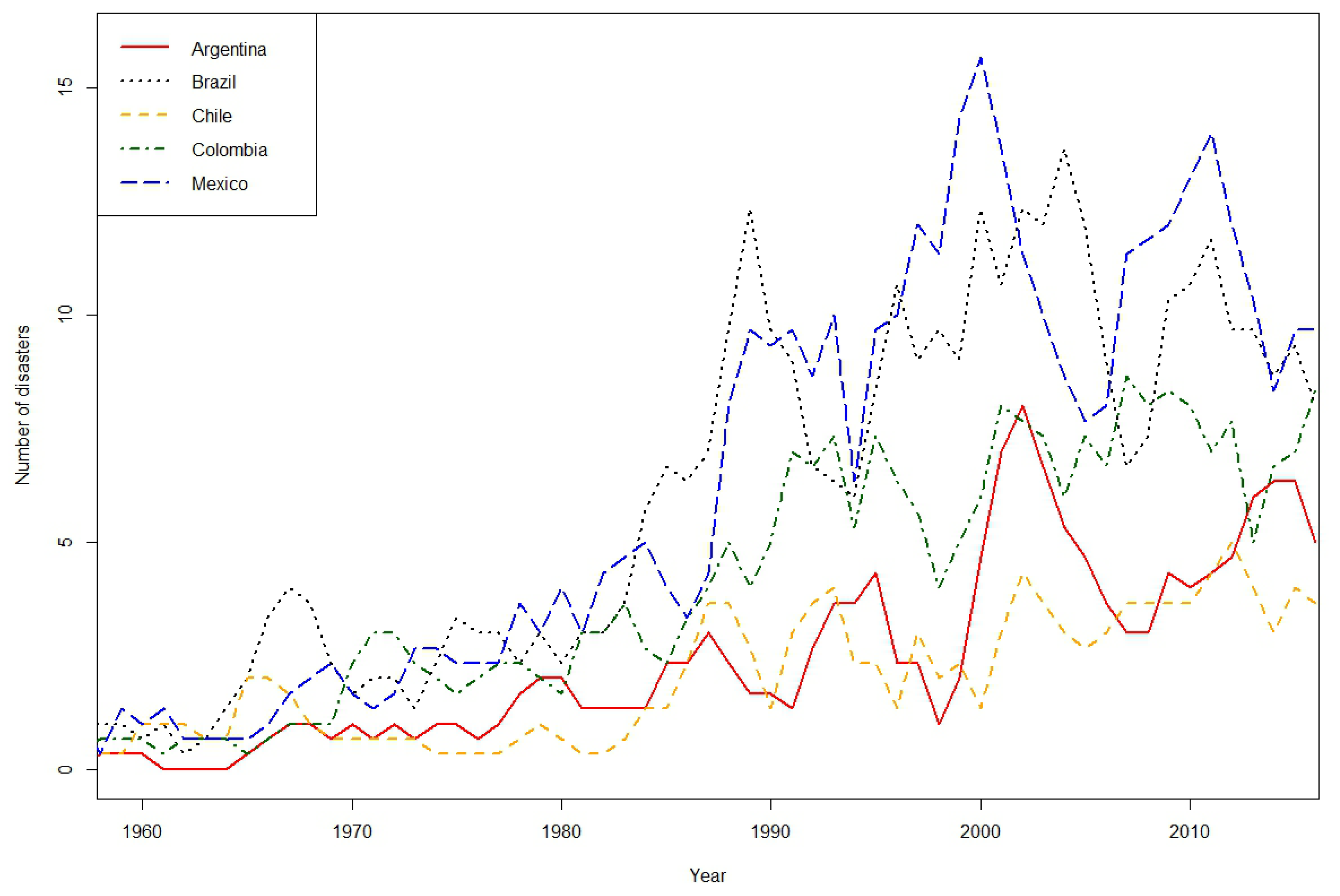
Figure 2.
Effect of a 1% increase in the probability of disaster in Argentina, Brazil, and Mexico. Calibration: see Table 1. Percentages on the vertical axis.
Figure 2.
Effect of a 1% increase in the probability of disaster in Argentina, Brazil, and Mexico. Calibration: see Table 1. Percentages on the vertical axis.
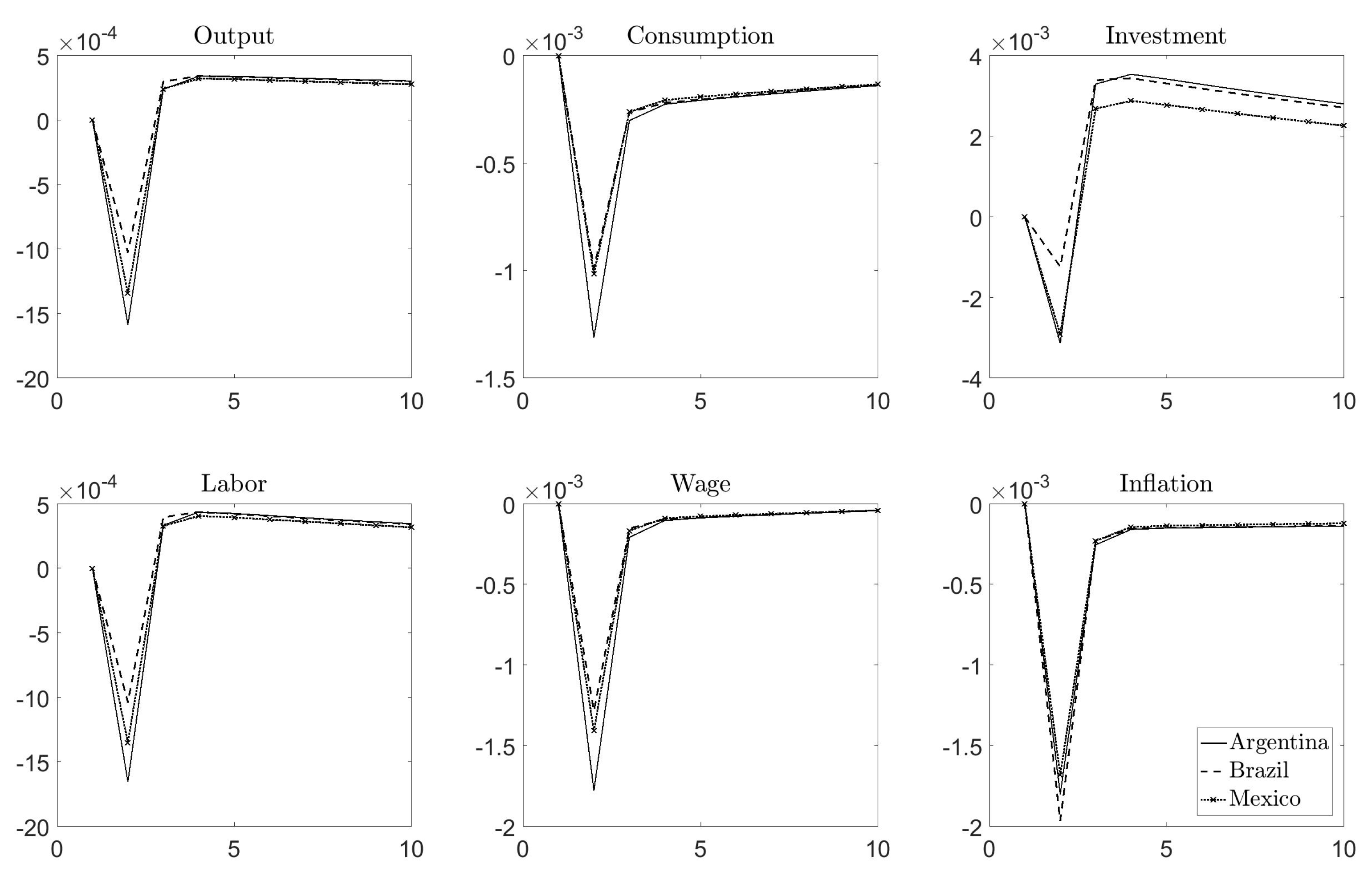
Figure 3.
Effect of a 1% increase in the probability of disaster in Chile and Colombia. Calibration: see Table 1. Percentages on the vertical axis.
Figure 3.
Effect of a 1% increase in the probability of disaster in Chile and Colombia. Calibration: see Table 1. Percentages on the vertical axis.
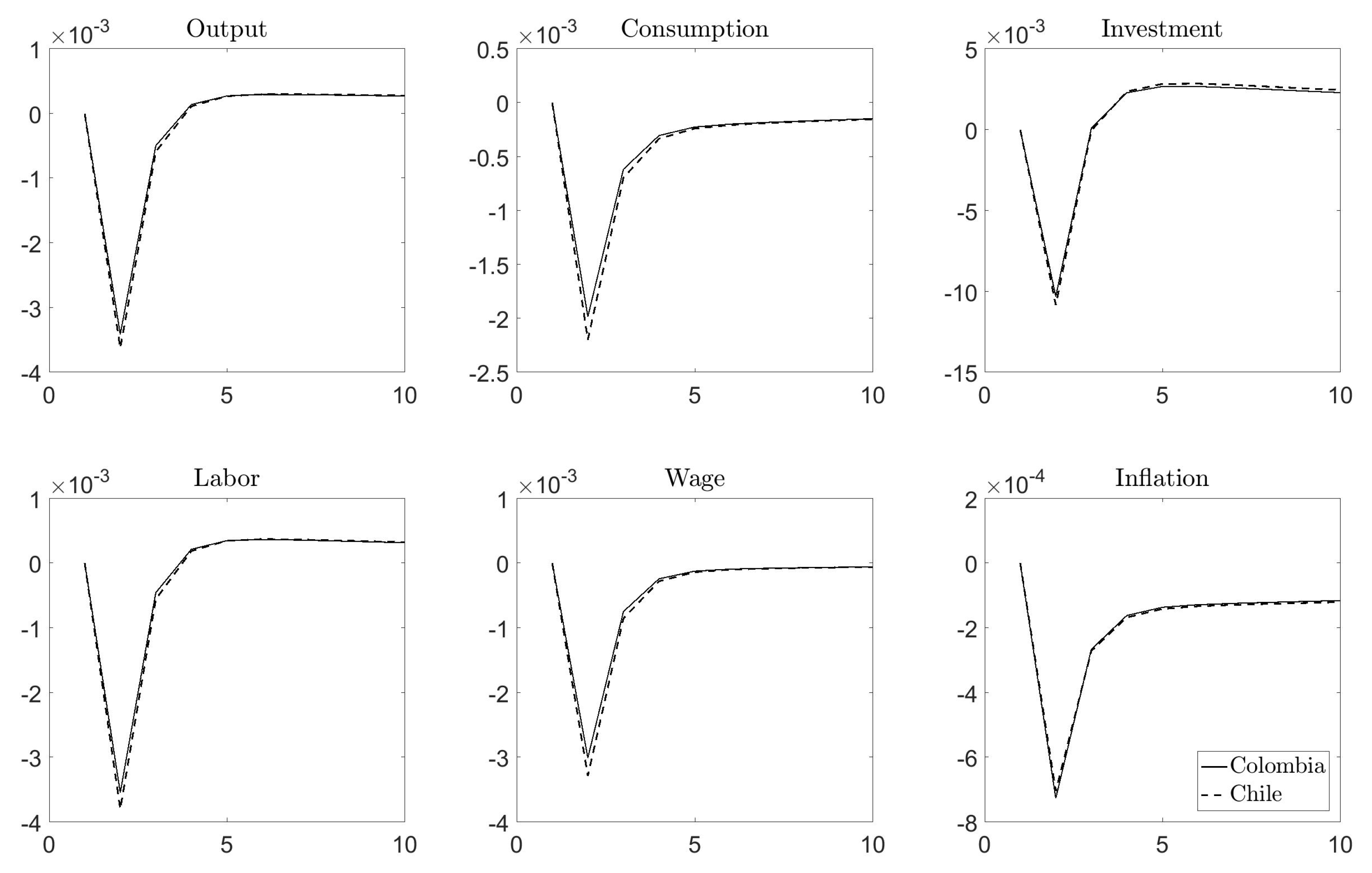
Figure 4.
Effect of a 1% increase in the probability of disaster in Argentina, Brazil, and Mexico, with varying steady-state disaster risk and size (see Table A1). Percentages on the vertical axis.
Figure 4.
Effect of a 1% increase in the probability of disaster in Argentina, Brazil, and Mexico, with varying steady-state disaster risk and size (see Table A1). Percentages on the vertical axis.

Figure 5.
Effect of a 1% increase in the probability of disaster in Chile and Colombia, with varying steady-state disaster risk and size (see Table A1). Percentages on the vertical axis.
Figure 5.
Effect of a 1% increase in the probability of disaster in Chile and Colombia, with varying steady-state disaster risk and size (see Table A1). Percentages on the vertical axis.
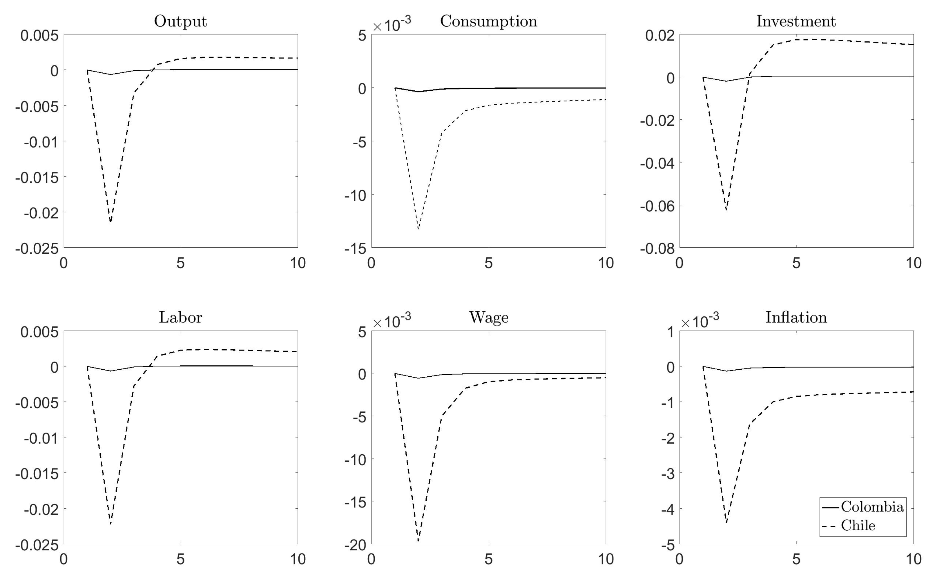
Table 1.
Calibration, monthly values.
| Disaster risk | ||
| probability of disaster | 0.0037 | |
| size of disaster | 0.0078 | |
| persistence of (log) disaster risk | 0.965 | |
| st. dev. of innovations to (log) disaster risk | 0.2 | |
| Utility function | ||
| discount factor | 0.9976 | |
| risk aversion coefficient | 3.8 | |
| leisure preference | 2.33 | |
| (Country-specific) EIS | ||
| Argentina | 0.1 | |
| Brazil | 0.107 | |
| Chile | 0.137 | |
| Colombia | 0.158 | |
| Mexico | 0.158 | |
| Investment | ||
| capital depreciation rate | 0.0067 | |
| capital adjustment cost | 2 | |
| steady-state utilization rate of capital | 1 | |
| Production | ||
| capital share of production | 0.33 | |
| elasticity of substitution among goods | 6 | |
| trend growth of productivity | 0.0017 | |
| (Country-specific) Calvo probability | ||
| Argentina | 0.41 | |
| Brazil | 0.33 | |
| Chile | 0.7 | |
| Colombia | 0.68 | |
| Mexico | 0.375 | |
| Public authority | ||
| Taylor rule inflation weight | 1.6 | |
| Taylor rule output weight | 0.4 | |
| target (gross) inflation rate | 1.0017 | |
| interest rate smoothing parameter | 0.947 |
© 2018 by the author. Licensee MDPI, Basel, Switzerland. This article is an open access article distributed under the terms and conditions of the Creative Commons Attribution (CC BY) license (http://creativecommons.org/licenses/by/4.0/).
Share and Cite
MDPI and ACS Style
Isoré, M. Changes in Natural Disaster Risk: Macroeconomic Responses in Selected Latin American Countries. Economies 2018, 6, 13. https://doi.org/10.3390/economies6010013
AMA Style
Isoré M. Changes in Natural Disaster Risk: Macroeconomic Responses in Selected Latin American Countries. Economies. 2018; 6(1):13. https://doi.org/10.3390/economies6010013
Chicago/Turabian StyleIsoré, Marlène. 2018. "Changes in Natural Disaster Risk: Macroeconomic Responses in Selected Latin American Countries" Economies 6, no. 1: 13. https://doi.org/10.3390/economies6010013
Note that from the first issue of 2016, this journal uses article numbers instead of page numbers. See further details here.