On Predictive Modeling Using a New Flexible Weibull Distribution and Machine Learning Approach: Analyzing the COVID-19 Data

Abstract

Predicting and modeling time-to-events data is a crucial and interesting research area. For modeling and predicting such types of data, numerous statistical models have been suggested and implemented. This study introduces a new statistical model, namely, a new modified flexible Weibull extension (NMFWE) distribution for modeling the mortality rate of COVID-19 patients. The introduced model is obtained by modifying the flexible Weibull extension model. The maximum likelihood estimators of the NMFWE model are obtained. The evaluation of the estimators of the NMFWE model is assessed in a simulation study. The flexibility and applicability of the NMFWE model are established by taking two datasets representing the mortality rates of COVID-19-infected persons in Mexico and Canada. For predictive modeling, we consider two pure statistical models and two machine learning (ML) algorithms. The pure statistical models include the autoregressive moving average (ARMA) and non-parametric autoregressive moving average (NP-ARMA), and the ML algorithms include neural network autoregression (NNAR) and support vector regression (SVR). To evaluate their forecasting performance, three standard measures of accuracy, namely, root mean square error (RMSE), mean absolute error (MAE), and mean absolute percentage error (MAPE) are calculated. The findings demonstrate that ML algorithms are very effective at predicting the mortality rate data.

1. Introduction

The coronavirus disease 2019 (COVID-19) pandemic has strongly affected the schedule of everyday life; particularly, it has created public health crises the likes of which we have never before faced. Biomedical researchers are constantly paying attention to estimating and predicting the average of new cases, the number or ratio of deaths, or the rate of recovery of the infected patients to make the appropriate arrangements (Hogan et al. [1]). In this regard, several studies on the COVID-19 pandemic have appeared. For example, Mizumoto et al. [2] estimated the asymptomatic proportion of COVID-19 cases in Japan. Ilyas et al. [3] studied the scenario of the COVID-19 pandemic in Pakistan. Rao et al. [4] investigated COVID-19 data using the Weibull distribution under indeterminacy. Up to 27 November 2021, 10:53 GMT, the total number of registered cases has reached 261 million, the total number of deaths around the globe has reached 5.2 million, and 235.86 million infected persons have recovered. Based on the latest updates about the COVID-19 pandemic, the United States of America is at the top of the list, having 49 million total cases and 799,138 deaths.

Several statistical models (SMs) have been implemented to describe, estimate, and predict the nature of the COVID-19 pandemic. For example, Singhal et al. [5] modeled and predicted the COVID-19 epidemic using the Gaussian model. Qin et al. [6] estimated the distribution of the incubation period of COVID-19 events. Almetwally et al. [7] implemented a new version of the inverted Topp–Leone (ITL) distribution to analyze the COVID-19 mortality rate. Almongy et al. [8] applied an extended version of the Rayleigh distribution to the COVID-19 data. Liu et al. [9] modeled the survival times of COVID-19-infected persons in China. El-Sagheer et al. [10] applied the mortality distribution to the COVID-19 data based on randomly censored observations.

In today’s competitive era, the data generated from various fields are becoming increasingly more complex. As a result, in modeling such data, we need machine learning tools under probability distributions that are best suited for analytical studies of multidimensional and complex data. Machine learning algorithms are often expressed in terms of probability; most machine learning tools are based on inferential statistics, where the statistics are based on probability theory. In essence, probability theory mathematically expresses how likely something is, given our assumptions. There are now probabilistic interpretations of black-box algorithms such as deep learning. These interpretations help us understand how such algorithms work, and how to improve them. There are many researchers who base their entire models for computer learning on statistics. At a basic level, they think that the world, or at least their problem, is driven by or best represented by certain combinations of random variables, which are best expressed by statistics. These models are typically suited to very different types of problems than are multifactor models. Furthermore, forecasting stock prices is a good example, where statistical models can be used for machine learning. Thus, machine learning is more linked to statistics and probabilities. See, for example, Eliwa et al. [11], El-Morshedy et al. [12,13], Altun et al. [14,15], among others.

In the current scenario, the best description of the COVID-19 pandemic is a crucial research topic. Several SMs are available that can be used to describe the behavior of the COVID-19 pandemic adequately, in addition to machine learning tools. Among the available SMs, the two-parameter flexible Weibull extension (FWE) model holds a key place (see Bebbington et al. [16]). Different variants of the FWE model have been introduced and implemented for dealing with the data in numerous sectors; see El-Morshedy et al. [17], El-Morshedy et al. [18], and Abubakari et al. [19].

Let a random variable $\mathit{W}$ have the FWE model with parameters ${\sigma }_1>0$ and ${\sigma }_2>0$; its cumulative distribution function (CDF) can be expressed as

$$K(w;{\sigma }_1,{\sigma }_2)=1-e^{-{\rm Y}(w;{\sigma }_1,{\sigma }_2)},w\ge 0,$$

(1)

with the probability density function (PDF) given by

$$k_{FWE}(w;{\sigma }_1,{\sigma }_2)=\left({\sigma }_1+\frac{{\sigma }_2}{w^2}\right){\rm Y}(w;{\sigma }_1,{\sigma }_2)e^{-{\rm Y}(w;{\sigma }_1,{\sigma }_2)},w>0,$$

where ${\rm Y}(w;{\sigma }_1,{\sigma }_2)=e^{{\sigma }_{1}w-\frac{{\sigma }_2}{w}}$. To add further flexibility to the FWE model, El-Gohary et al. [20] proposed the exponentiated FWE (Exp-FWE) model with parameters ${\sigma }_1>0,$ ${\sigma }_2>0$, and ${\delta }_1>0$. The CDF of the Exp-FWE model is given by

$$K(w;{\sigma }_1,{\sigma }_2,{\delta }_1)={\left(1-e^{-{\rm Y}(w;{\sigma }_1,{\sigma }_2)}\right)}^{{\delta }_1},w\ge 0.$$

El-Damcese et al. [21] further modified the Exp-FWE model by introducing the Kumaramswamy FWE (Ku-FWE) model with parameters ${\sigma }_1>0, {\sigma }_2>0, {\delta }_1$, and ${\delta }_2>0$. The CDF $K(w;{\sigma }_1,{\sigma }_2,{\delta }_1,{\delta }_2)$ of the Ku-FWE model is given by

$$K(w;{\sigma }_1,{\sigma }_2,{\delta }_1,{\delta }_2)=1-{\left(1-{\left[1-e^{-{\rm Y}(w;{\sigma }_1,{\sigma }_2)}\right]}^{{\delta }_1}\right)}^{{\delta }_2},w\ge 0.$$

Recently, Ahmad et al. [22] further contributed to this research area by proposing a new family of distributions with CDF, given by

$$M\left(w;\lambda ,\mathbf{\vartheta }\right)=\frac{\lambda K\left(w;\mathbf{\vartheta }\right)}{\lambda -1+K\left(w;\mathbf{\vartheta }\right)},w\in \mathbb{R},\lambda >1,$$

(2)

where $K\left(w;\mathbf{\vartheta }\right)$ is the CDF of the baseline model with parameter vector $\mathbf{\vartheta }$. The corresponding PDF, survival function (SF), and hazard function (HF) to Equation (2) are given by

$$m\left(w;\lambda ,\mathbf{\vartheta }\right)=\frac{\lambda (\lambda -1)k\left(w;\mathbf{\vartheta }\right)}{{\left[\lambda -1+K\left(w;\mathbf{\vartheta }\right)\right]}^2},w\in \mathbb{R},$$

$$S\left(w;\lambda ,\mathbf{\vartheta }\right)=1-\frac{\lambda K\left(w;\mathbf{\vartheta }\right)}{\lambda -1+K\left(w;\mathbf{\vartheta }\right)},w\in \mathbb{R},$$

and

$$h\left(w;\lambda ,\mathbf{\vartheta }\right)=\frac{\lambda k\left(w;\mathbf{\vartheta }\right)}{(1-K\left(w;\mathbf{\vartheta }\right))\left[\lambda -1+K\left(w;\mathbf{\vartheta }\right)\right]},w\in \mathbb{R},$$

respectively.

As we know, heavy-tailed (HT) distributions play a vital role in medical and other related sectors ((Gardiner et al. [23]), (Zhao et al. [24])). However, in the literature, there are only few distributions that possess the HT characteristics ((Bhati and Ravi, [25]), (Ahmad et al. [26]), (Ahmad et al. [27])). Keeping in view the importance of the HT distributions, we introduce a new HT distribution, namely, a new modified flexible Weibull extension (NMFWE) distribution. The HT characteristics of the NMFWE distributions are proved mathematically (see Section 3). The NMFWE distribution is introduced by incorporating $K(w;{\sigma }_1,{\sigma }_2)=1-e^{-{\rm Y}(w;{\sigma }_1,{\sigma }_2)}$ in Equation (2).

2. A New Modified Flexible Weibull Extension

A random variable $\mathit{W}$ has the NMFWE distribution with parameters $\lambda >1,{\sigma }_1>0$, and ${\sigma }_2>0$, if its CDF can be formulated as

$$M\left(w;\lambda ,{\sigma }_1,{\sigma }_2\right)=\frac{\lambda -\lambda e^{-{\rm Y}(w;{\sigma }_1,{\sigma }_2)}}{\lambda -e^{-{\rm Y}(w;{\sigma }_1,{\sigma }_2)}},w\ge 0.$$

(3)

In link to $M\left(w;\lambda ,{\sigma }_1,{\sigma }_2\right)$, the PDF and HF can be expressed as

$$m\left(w;\lambda ,{\sigma }_1,{\sigma }_2\right)=\frac{\lambda (\lambda -1)\left({\sigma }_1+\frac{{\sigma }_2}{w^2}\right){\rm Y}(w;{\sigma }_1,{\sigma }_2)e^{-{\rm Y}(w;{\sigma }_1,{\sigma }_2)}}{{\left[\lambda -e^{-{\rm Y}(w;{\sigma }_1,{\sigma }_2)}\right]}^2},w>0,$$

(4)

and

$$h\left(w;\lambda ,{\sigma }_1,{\sigma }_2\right)=\frac{\lambda \left({\sigma }_1+\frac{{\sigma }_2}{w^2}\right){\rm Y}(w;{\sigma }_1,{\sigma }_2)}{\lambda -e^{-{\rm Y}(w;{\sigma }_1,{\sigma }_2)}},w>0,$$

respectively.

For different values of $\lambda ,{\sigma }_1$, and ${\sigma }_2$, visual illustrations of $m\left(w;\lambda ,{\sigma }_1,{\sigma }_2\right)$, and $h\left(w;\lambda ,{\sigma }_1,{\sigma }_2\right)$ are presented in Figure 1.

It is found that the proposed model can be used effectively in modeling symmetric and asymmetric data. Moreover, it can be utilized as a probability tool to discuss various kinds of failure rates.

3. The HT Characteristics

This section is devoted to proving the HT characteristics of the NMFWE distribution.

Regular Variational Property

Here, we prove the regular variational property of the NMFWE distribution. According to Seneta [28], in terms of SF $S\left(w;\mathbf{\vartheta }\right)=1-K\left(w;\mathbf{\vartheta }\right)$, we have:

Theorem 1.

If $\left[1-K\left(w;\mathbf{\vartheta }\right)\right]$ is the SF of the regular varying distribution (RVD), then $[1-M$$(w;\lambda ,{\sigma }_1,{\sigma }_2)]$ is an RVD.

Proof. 

Suppose ${lim}_{w\to \infty }\frac{\left[1-K\left(aw;\mathbf{\vartheta }\right)\right]}{\left[1-K\left(w;\mathbf{\vartheta }\right)\right]}=f\left(w\right)$ is finite but nonzero for every $w>0$. Incorporating Equation (5), we obtain

$$\underset{w\to \infty }{lim}\frac{1-M\left(aw;\lambda ,{\sigma }_1,{\sigma }_2\right)}{1-M\left(w;\lambda ,{\sigma }_1,{\sigma }_2\right)}=\underset{w\to \infty }{lim}\frac{\left(\lambda -1\right)\left[1-K\left(aw;\mathbf{\vartheta }\right)\right]}{\lambda -1+K\left(aw;\mathbf{\vartheta }\right)}\times \frac{\lambda -1+K\left(w;\mathbf{\vartheta }\right)}{\left(\lambda -1\right)\left[1-K\left(w;\mathbf{\vartheta }\right)\right]},$$

$$\underset{w\to \infty }{lim}\frac{1-M\left(aw;\lambda ,{\sigma }_1,{\sigma }_2\right)}{1-M\left(w;\lambda ,{\sigma }_1,{\sigma }_2\right)}=\underset{w\to \infty }{lim}\frac{\left[1-K\left(aw;\mathbf{\vartheta }\right)\right]}{\left[1-K\left(w;\mathbf{\vartheta }\right)\right]}\times \frac{\lambda -1+K\left(w;\mathbf{\vartheta }\right)}{\lambda -1+K\left(aw;\mathbf{\vartheta }\right)},$$

$$\underset{w\to \infty }{lim}\frac{1-M\left(aw;\lambda ,{\sigma }_1,{\sigma }_2\right)}{1-M\left(w;\lambda ,{\sigma }_1,{\sigma }_2\right)}=\underset{w\to \infty }{lim}f\left(w\right)\times \frac{\lambda -1+K\left(w;\mathbf{\vartheta }\right)}{\lambda -1+K\left(aw;\mathbf{\vartheta }\right)}.$$

(5)

Using Equation (3) in Equation (5), we obtain

$$\underset{w\to \infty }{lim}\frac{1-M\left(aw;\lambda ,{\sigma }_1,{\sigma }_2\right)}{1-M\left(w;\lambda ,{\sigma }_1,{\sigma }_2\right)}=\underset{w\to \infty }{lim}f\left(w\right)\times \frac{\lambda -1+\left(1-e^{-e^{{\sigma }_{1}w-\frac{{\sigma }_2}{w}}}\right)}{\lambda -1+\left(1-e^{-e^{{\sigma }_1\left(aw\right)-\frac{{\sigma }_2}{\left(aw\right)}}}\right)},$$

$$\underset{w\to \infty }{lim}\frac{1-M\left(aw;\lambda ,{\sigma }_1,{\sigma }_2\right)}{1-M\left(w;\lambda ,{\sigma }_1,{\sigma }_2\right)}=\underset{w\to \infty }{lim}f\left(w\right)\times \frac{\lambda -1+\left(1-e^{-e^{{\sigma }_1\times \infty -\frac{{\sigma }_2}{\infty }}}\right)}{\lambda -1+\left(1-e^{-e^{{\sigma }_1(a\times \infty )-\frac{{\sigma }_2}{(a\times \infty )}}}\right)},$$

$$\underset{w\to \infty }{lim}\frac{1-M\left(aw;\lambda ,{\sigma }_1,{\sigma }_2\right)}{1-M\left(w;\lambda ,{\sigma }_1,{\sigma }_2\right)}=\underset{w\to \infty }{lim}f\left(w\right)\times \frac{\lambda -1+\left(1-e^{-e^{\infty }}\right)}{\lambda -1+\left(1-e^{-e^{\infty }}\right)},$$

$$\underset{w\to \infty }{lim}\frac{1-M\left(aw;\lambda ,{\sigma }_1,{\sigma }_2\right)}{1-M\left(w;\lambda ,{\sigma }_1,{\sigma }_2\right)}=\underset{w\to \infty }{lim}f\left(w\right)\times \frac{\lambda -1+\left(1-e^{-\infty }\right)}{\lambda -1+\left(1-e^{-\infty }\right)},$$

$$\underset{w\to \infty }{lim}\frac{1-M\left(aw;\lambda ,{\sigma }_1,{\sigma }_2\right)}{1-M\left(w;\lambda ,{\sigma }_1,{\sigma }_2\right)}=\underset{w\to \infty }{lim}f\left(w\right)\times \frac{\lambda -1+\left(1-\frac{1}{e^{\infty }}\right)}{\lambda -1+\left(1-\frac{1}{e^{\infty }}\right)},$$

$$\underset{w\to \infty }{lim}\frac{1-M\left(aw;\lambda ,{\sigma }_1,{\sigma }_2\right)}{1-M\left(w;\lambda ,{\sigma }_1,{\sigma }_2\right)}=\underset{w\to \infty }{lim}f\left(w\right)\times \frac{\lambda -1+1}{\lambda -1+1},$$

$$\underset{w\to \infty }{lim}\frac{1-M\left(aw;\lambda ,{\sigma }_1,{\sigma }_2\right)}{1-M\left(w;\lambda ,{\sigma }_1,{\sigma }_2\right)}=\underset{w\to \infty }{lim}f\left(w\right).$$

(6)

Since Equation (6) is nonzero for every $w>0$, $\left[1-M\left(w;\lambda ,{\sigma }_1,{\sigma }_2\right)\right]$ is the SF of the RVD. □

A Supportive Example of RVP

Suppose W follows a power-law behavior; then, as per the definition of the HT property, we have

$$1-K\left(w;\mathbf{\vartheta }\right)=\mathbb{P}(W>w)\sim w^{-\beta }.$$

By implementing Karamata’s characterization theorem (Seneta, [28]), we can write the expression $\left[1-M\left(aw;\lambda ,{\sigma }_1,{\sigma }_2\right)\right]$ as

$$1-M\left(w;\lambda ,{\sigma }_1,{\sigma }_2\right)=w^{-\beta }L\left(w\right),$$

where the quantity $L\left(w\right)$ represents the slowly varying function (SVF). From Equation (5), we have

$$1-M\left(w;\lambda ,{\sigma }_1,{\sigma }_2\right)=\frac{\left[1-K\left(w;\mathbf{\vartheta }\right)\right]\left(\lambda -1\right)}{\lambda -1+K\left(w;\mathbf{\vartheta }\right)},$$

$$1-M\left(w;\lambda ,{\sigma }_1,{\sigma }_2\right)=\frac{w^{-\beta }\left(\lambda -1\right)}{\lambda -1+K\left(w;\mathbf{\vartheta }\right)},$$

$$1-M\left(w;\lambda ,{\sigma }_1,{\sigma }_2\right)=w^{-\beta }L\left(w\right),$$

(7)

where $L\left(w\right)=\frac{\left(\lambda -1\right)}{\lambda -1+K\left(w;\mathbf{\vartheta }\right)}$. If we can show that $L\left(w\right)$ is an SVF, then the result obtained in Equation (7) is true. To show $L\left(w\right)$ is an SVF, we must satisfy

$$\underset{z\to \infty }{lim}\frac{L\left(aw\right)}{L\left(w\right)}=1.$$

So,

$$\frac{L\left(aw\right)}{L\left(w\right)}=\frac{\frac{\left(\lambda -1\right)}{\lambda -1+K\left(aw;\mathbf{\vartheta }\right)}}{\frac{\left(\lambda -1\right)}{\lambda -1+K\left(w;\mathbf{\vartheta }\right)}},$$

$$\frac{L\left(aw\right)}{L\left(w\right)}=\frac{\lambda -1+K\left(w;\mathbf{\vartheta }\right)}{\lambda -1+K\left(aw;\mathbf{\vartheta }\right)},$$

$$\frac{L\left(aw\right)}{L\left(w\right)}=\frac{\lambda -1+\left(1-e^{-e^{{\sigma }_1\times w-\frac{{\sigma }_2}{w}}}\right)}{\lambda -1+\left(1-e^{-e^{{\sigma }_1(a\times w)-\frac{{\sigma }_2}{a\times w}}}\right)}.$$

Applying the limit, we obtain

$$\underset{w\to \infty }{lim}\frac{L\left(aw\right)}{L\left(w\right)}=\frac{\lambda -1+\left(1-e^{-e^{{\sigma }_1\times \infty -\frac{{\sigma }_2}{\infty }}}\right)}{\lambda -1+\left(1-e^{-e^{{\sigma }_1(a\times \infty )-\frac{{\sigma }_2}{a\times \infty }}}\right)},$$

$$\underset{w\to \infty }{lim}\frac{L\left(aw\right)}{L\left(w\right)}=\frac{\lambda -1+1}{\lambda -1+1},$$

$$\underset{w\to \infty }{lim}\frac{L\left(aw\right)}{L\left(w\right)}=1.$$

4. Estimation and Simulation

In this section, we adopt a known estimation procedure to obtain the maximum likelihood estimators (MLEs) $\left(\widehat{{\sigma }_1},\widehat{{\sigma }_2},\widehat{\lambda }\right)$ of the parameters $\left({\sigma }_1,{\sigma }_2,\lambda \right)$. After obtaining the MLEs of the parameters, we conduct a simulation study (SimS) to assess the performances of the estimators.

Let $W_1,W_2,\cdots ,W_n$ be an observed random sample (RS) of size $\mathit{n}$, taken from $m\left(w;\lambda ,{\sigma }_1,{\sigma }_2\right)$. In link to $m\left(w;\lambda ,{\sigma }_1,{\sigma }_2\right)$, the likelihood function (LiF), say $\Delta \left(\lambda ,{\sigma }_1,{\sigma }_2|w_1,w_2,\cdots ,w_n\right)$, is given by

$$\Delta \left(\lambda ,{\sigma }_1,{\sigma }_2|w_1,w_2,\cdots ,w_n\right)=\prod _{a=1}^n\frac{\lambda (\lambda -1)\left({\sigma }_1+\frac{{\sigma }_2}{w_a^2}\right){{\rm Y}}_a(w_a;{\sigma }_1,{\sigma }_2)e^{-{{\rm Y}}_a(w_a;{\sigma }_1,{\sigma }_2)}}{{\left[\lambda -e^{-{{\rm Y}}_a(w_a;{\sigma }_1,{\sigma }_2)}\right]}^2},$$

(8)

where ${{\rm Y}}_a(w_a;{\sigma }_1,{\sigma }_2)=e^{{\sigma }_1{w}_a-\frac{{\sigma }_2}{w_a}}$. The corresponding log LiF to $\Delta \left(\lambda ,{\sigma }_1,{\sigma }_2|w_1,w_2,\cdots ,w_n\right)$ can be formulated as

$$\begin{array}{cc}\hfill \delta \left(\lambda ,{\sigma }_1,{\sigma }_2|w_1,w_2,\cdots ,w_n\right)& =nlog\lambda +nlog\left(1-\lambda \right)+\sum _{a=1}^{n}log\left({\sigma }_1+\frac{{\sigma }_2}{w_a^2}\right)+\sum _{a=1}^n{\sigma }_1{w}_a\hfill \\ \hfill & -\sum _{a=1}^n\frac{{\sigma }_2}{w_a}-\sum _{a=1}^n{{\rm Y}}_a(w_a;{\sigma }_1,{\sigma }_2)-2\sum _{a=1}^{n}log\left[\lambda -e^{-{{\rm Y}}_a(w_a;{\sigma }_1,{\sigma }_2)}\right].\hfill \end{array}$$

Based on $\delta \left(\lambda ,{\sigma }_1,{\sigma }_2|w_1,w_2,\cdots ,w_n\right)$, the partial derivatives are given by

$$\begin{array}{cc}\hfill \frac{\partial }{\partial {\sigma }_1}\delta \left(\lambda ,{\sigma }_1,{\sigma }_2|w_1,w_2,\cdots ,w_n\right)& =\sum _{a=1}^n\frac{1}{\left({\sigma }_1+\frac{{\sigma }_2}{w_a^2}\right)}+\sum _{a=1}^n{w}_a-\sum _{a=1}^n{w}_a{{\rm Y}}_a(w_a;{\sigma }_1,{\sigma }_2)\hfill \\ \hfill & -2\sum _{a=1}^n\frac{w_a{{\rm Y}}_a(w_a;{\sigma }_1,{\sigma }_2)e^{-{{\rm Y}}_a(w_a;{\sigma }_1,{\sigma }_2)}}{\left[\lambda -e^{-{{\rm Y}}_a(w_a;{\sigma }_1,{\sigma }_2)}\right]},\hfill \end{array}$$

$$\begin{array}{cc}\hfill \frac{\partial }{\partial {\sigma }_2}\delta \left(\lambda ,{\sigma }_1,{\sigma }_2|w_1,w_2,\cdots ,w_n\right)& =\sum _{a=1}^n\frac{\frac{1}{w_a}}{\left({\sigma }_1+\frac{{\sigma }_2}{w_a^2}\right)}-\sum _{a=1}^n\frac{1}{w_a}+\sum _{a=1}^n\frac{1}{w_a}{{\rm Y}}_a(w_a;{\sigma }_1,{\sigma }_2)\hfill \\ \hfill & +2\sum _{a=1}^n\frac{\frac{1}{w_a}{{\rm Y}}_a(w_a;{\sigma }_1,{\sigma }_2)e^{-{{\rm Y}}_a(w_a;{\sigma }_1,{\sigma }_2)}}{\left[\lambda -e^{-{{\rm Y}}_a(w_a;{\sigma }_1,{\sigma }_2)}\right]},\hfill \end{array}$$

and

$$\frac{\partial }{\partial \lambda }\delta \left(\lambda ,{\sigma }_1,{\sigma }_2|w_1,w_2,\cdots ,w_n\right)=\frac{n}{\lambda }+\frac{n}{\left(1-\lambda \right)}-2\sum _{a=1}^n\frac{1}{\left[\lambda -e^{-{{\rm Y}}_a(w_a;{\sigma }_1,{\sigma }_2)}\right]},$$

respectively.

Solving $\frac{\partial }{\partial {\sigma }_1}\delta \left(\lambda ,{\sigma }_1,{\sigma }_2|w_1,w_2,\cdots ,w_n\right)=0$, $\frac{\partial }{\partial {\sigma }_2}\delta \left(\lambda ,{\sigma }_1,{\sigma }_2|w_1,w_2,\cdots ,w_n\right)=0$, and $\frac{\partial }{\partial \lambda }\delta \left(\lambda ,{\sigma }_1,{\sigma }_2|w_1,w_2,\cdots ,w_n\right)=0$ yields $\widehat{{\sigma }_1},\widehat{{\sigma }_2}$, and $\widehat{\lambda }$, respectively.

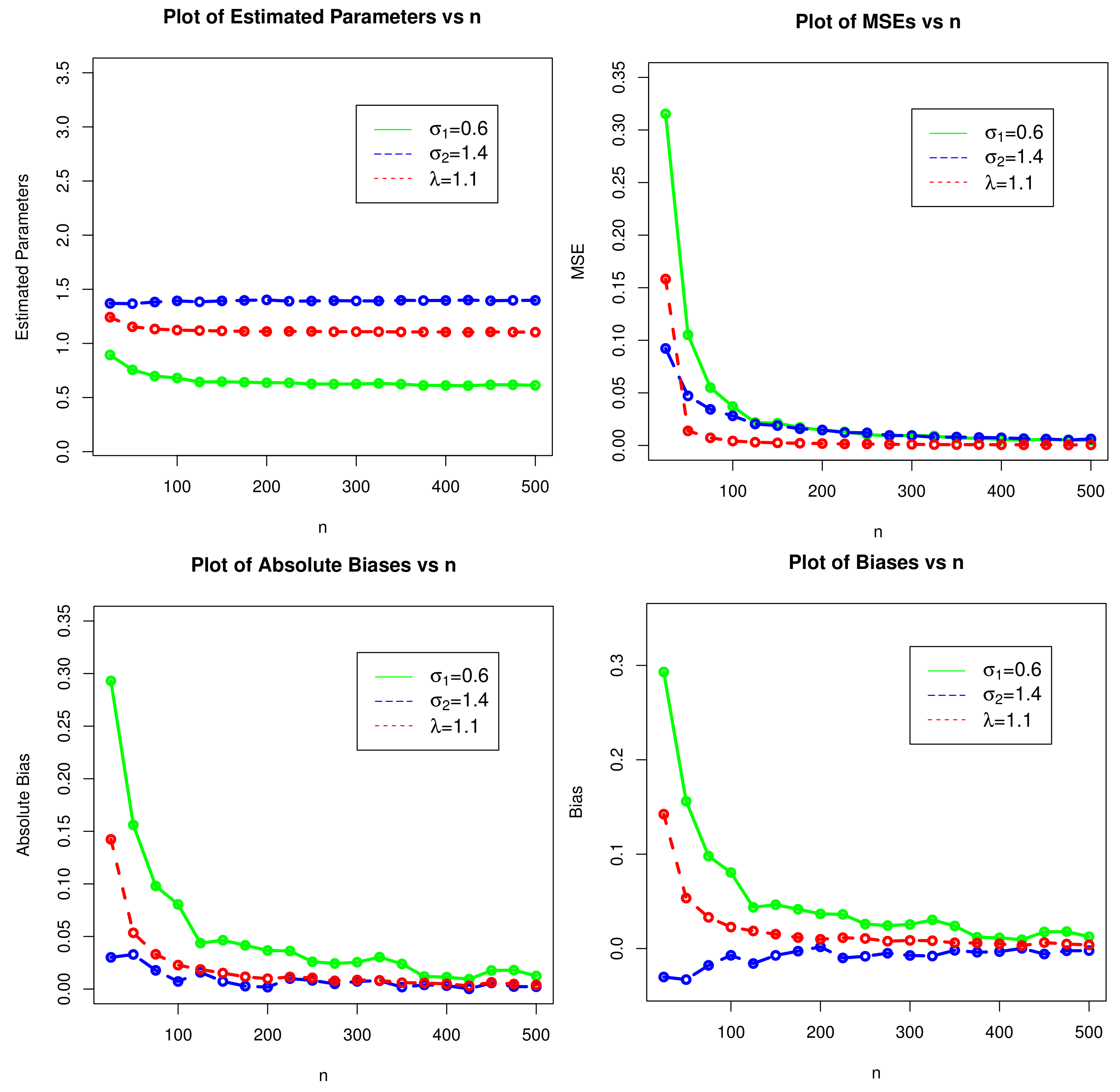
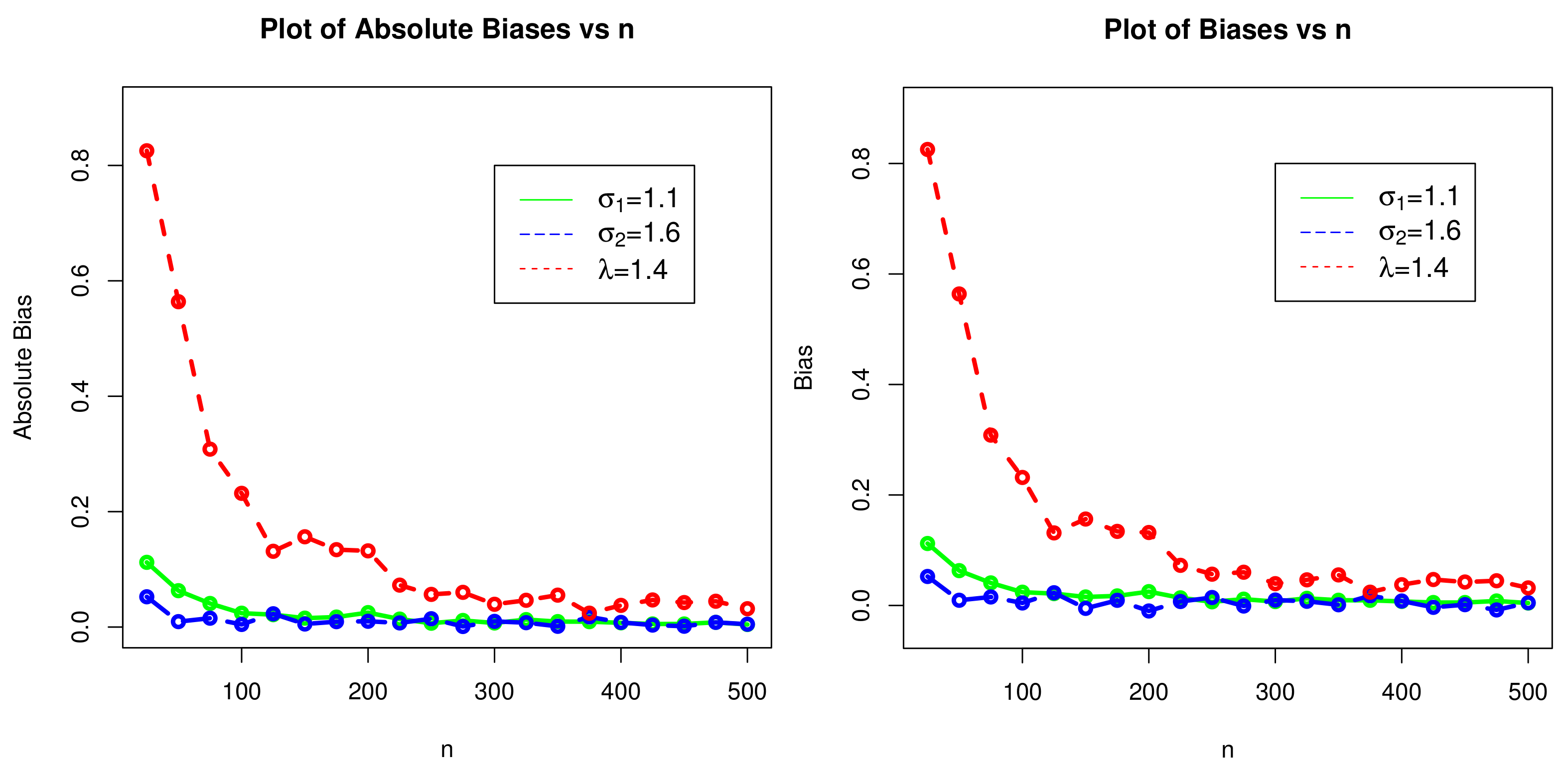
Next, we assess the performances of $\widehat{{\sigma }_1},\widehat{{\sigma }_2}$, and $\widehat{\lambda }$ via an SimS. For carrying out the SimS, an RS, say $n=25,50,\cdots ,500$, was obtained from the NMFWE model. The SimS was performed for two schemes as follows: scheme I: ${\sigma }_1=0.6,{\sigma }_2=1.4,\lambda =1.1)$; scheme II: ${\sigma }_1=1.1,{\sigma }_2=1.6,\lambda =1.4$. Furthermore, two evaluation criteria, bias and mean square error (MSE), were considered for assessing $\widehat{{\sigma }_1},\widehat{{\sigma }_2}$, and $\widehat{\lambda }$. These criteria were, respectively, computed using the below expressions:

$$Bias\left(\widehat{\Theta }\right)=\frac{1}{n}\sum _{a=1}^n\left(\widehat{\Theta }-\Theta \right),$$

and

$$MSE\left(\widehat{\Theta }\right)=\frac{1}{n}\sum _{a=1}^n{\left(\widehat{\Theta }-\Theta \right)}^2,$$

where $\Theta =\left({\sigma }_1,{\sigma }_2,\lambda \right)$.

Corresponding to scheme I, the results of the SimS are provided in

Table 1. The results of the SimS of the NMFWE model for ${\sigma }_1=0.6,{\sigma }_2=1.4$, and $\lambda =1.1$.

n	Parameters	MLEs	MSEs	Biases
	${\sigma }_1$	0.89302560	0.315274822	0.293025560
25	${\sigma }_2$	1.36985000	0.092232346	−0.03015010
	$\lambda$	1.24237000	0.158247051	0.142369775
	${\sigma }_1$	0.75604460	0.105204950	0.156044587
50	${\sigma }_2$	1.36711800	0.047163494	−0.03288202
	$\lambda$	1.15347600	0.013885900	0.053475874
	${\sigma }_1$	0.69801090	0.055053130	0.098010942
75	${\sigma }_2$	1.38220000	0.034336224	−0.01779995
	$\lambda$	1.13308800	0.007274670	0.033088078
	${\sigma }_1$	0.68048360	0.037073941	0.080483598
100	${\sigma }_2$	1.39280200	0.028143866	−0.00719760
	$\lambda$	1.12277300	0.004239282	0.022773367
	${\sigma }_1$	0.64644740	0.021180684	0.046447381
150	${\sigma }_2$	1.39273800	0.018909237	−0.00726232
	$\lambda$	1.11521500	0.002497769	0.015214547
	${\sigma }_1$	0.63668930	0.014568689	0.036689263
200	${\sigma }_2$	1.40180900	0.014734874	0.001809424
	$\lambda$	1.10985700	0.001831123	0.009857116
	${\sigma }_1$	0.62596330	0.010368965	0.025963329
250	${\sigma }_2$	1.39177300	0.011995360	−0.00822708
	$\lambda$	1.11065800	0.001393079	0.010658350
	${\sigma }_1$	0.62550910	0.009587663	0.025509126
300	${\sigma }_2$	1.39270200	0.009345810	−0.00729828
	$\lambda$	1.10861100	0.001066879	0.008610622
	${\sigma }_1$	0.62391800	0.006948299	0.023917996
350	${\sigma }_2$	1.39811500	0.008009759	−0.00188529
	$\lambda$	1.10609300	0.000808322	0.006093125
	${\sigma }_1$	0.61132940	0.005626040	0.011329370
400	${\sigma }_2$	1.39673000	0.007298053	−0.00327033
	$\lambda$	1.10493100	0.000693269	0.004930592
	${\sigma }_1$	0.61765410	0.005751539	0.017654106
450	${\sigma }_2$	1.39418200	0.006140556	−0.00581764
	$\lambda$	1.10637100	0.000606152	0.006371330
	${\sigma }_1$	0.61250040	0.004853576	0.012500388
500	${\sigma }_2$	1.39779400	0.006180866	−0.00220605
	$\lambda$	1.10388200	0.000549189	0.003882268

and presented visually in Figure 2, whereas

Table 2. The results of the SimS of the NMFWE model for ${\sigma }_1=1.1,{\sigma }_2=1.6$, and $\lambda =1.4$.

n	Parameters	MLEs	MSEs	Biases
	${\sigma }_1$	1.21214000	0.109696162	0.112139576
25	${\sigma }_2$	1.65247100	0.211066950	0.052471477
	$\lambda$	2.22540700	2.677630360	0.825406630
	${\sigma }_1$	1.16302800	0.046138277	0.063028001
50	${\sigma }_2$	1.60940600	0.127701240	0.009405599
	$\lambda$	1.96382400	1.630116700	0.563823750
	${\sigma }_1$	1.14084100	0.029142804	0.040841203
75	${\sigma }_2$	1.61535700	0.080794640	0.015357220
	$\lambda$	1.70831400	0.785862990	0.308313730
	${\sigma }_1$	1.12400600	0.018225475	0.024006192
100	${\sigma }_2$	1.60450400	0.065363500	0.004504030
	$\lambda$	1.63171300	0.494613440	0.231713380
	${\sigma }_1$	1.11539700	0.012912002	0.015397237
150	${\sigma }_2$	1.59474700	0.048261320	−0.005252810
	$\lambda$	1.55643900	0.268352060	0.156439100
	${\sigma }_1$	1.12505500	0.009975488	0.025054780
200	${\sigma }_2$	1.59002600	0.031762970	−0.00997431
	$\lambda$	1.53205300	0.172517940	0.132052860
	${\sigma }_1$	1.10665200	0.007469320	0.006651779
250	${\sigma }_2$	1.61439400	0.028265080	0.014393549
	$\lambda$	1.45660500	0.079107080	0.056605210
	${\sigma }_1$	1.10702000	0.005739174	0.007019600
300	${\sigma }_2$	1.60981400	0.022193800	0.009813938
	$\lambda$	1.43945700	0.037317540	0.039456630
	${\sigma }_1$	1.10944500	0.005131958	0.009445283
350	${\sigma }_2$	1.60127800	0.019648730	0.001277727
	$\lambda$	1.45528500	0.056621610	0.055285400
	${\sigma }_1$	1.10729900	0.004561712	0.007299329
400	${\sigma }_2$	1.60803700	0.017440070	0.008037465
	$\lambda$	1.43753900	0.036744330	0.037538550
	${\sigma }_1$	1.10532200	0.003908403	0.005322438
450	${\sigma }_2$	1.60144000	0.016748580	0.001439921
	$\lambda$	1.44244400	0.033483900	0.042444350
	${\sigma }_1$	1.10438500	0.003518714	0.004384936
500	${\sigma }_2$	1.60492800	0.013190150	0.004928443
	$\lambda$	1.43178200	0.024440440	0.031781690

(numerical illustration) and Figure 3 (visual illustration) offer the results of the SimS for schema II. The SimS was performed with the objective that (i) as the value of $\mathit{n}$ increases, the values of $\widehat{{\sigma }_1},\widehat{{\sigma }_2}$, and $\widehat{\lambda }$ tend to stability, and (ii), the biases and mean square errors tend to zero as the sample size grows; this proves the consistency property for the estimators. Thus, we can conclude that the maximum likelihood approach works quite well in estimating the model parameters under various sample sizes.

5. Data Analysis

This section deals with data analysis to illustrate the crucial and important role of the NMFWE model in real life data modeling. To show the applicability of the NMFWE model and to carry out its illustration, two datasets from the health sector are considered. The first dataset (Data 1) consists of 106 observations and represents the mortality rate of patients during the COVID-19 pandemic in Mexico. The second dataset (Data 2) consists of 224 observations and represents the mortality rate of patients during the COVID-19 pandemic in Canada. Both datasets are provided in

Table 3. The COVID-19 datasets.

Data 1

1.7652, 1.2210, 1.8782, 2.9924, 2.0766, 1.4534, 2.6440, 3.2996, 2.3330, 1.2030, 2.1710, 1.2244, 1.3312, 0.6880, 1.1708, 2.1370, 2.0070, 1.0484, 0.8688, 1.0286, 1.5260, 2.9208, 1.5806, 1.2740, 0.7074, 1.2654, 0.9460, 0.6430, 1.8568, 2.5756, 1.7626, 2.0086, 1.4520, 1.1970, 1.2824, 0.6790, 0.8848, 1.9870, 1.5680, 1.9100, 0.6998, 0.7502, 1.3936, 0.6572, 2.0316, 1.6216, 1.3394, 1.4302, 1.3120, 0.4154, 0.7556, 0.5976, 0.6672, 1.3628, 1.6650, 1.5708, 1.7102, 0.6456, 1.4972, 1.3250, 1.2280, 0.9818, 0.9322, 1.0784, 2.4084, 1.7392, 0.3630, 0.6654, 1.0812, 1.2364, 0.2082, 0.3600, 0.9898, 0.8178, 0.6718, 0.4140, 0.6596, 1.0634, 1.0884, 0.9114, 0.8584, 0.5000, 1.3070, 0.9296, 0.9394, 1.0918, 0.8240, 0.7844, 0.6438, 0.2804, 0.4876, 0.6514, 0.7264, 0.6466, 0.6054, 0.4704, 0.2410, 0.6436, 0.5852, 0.5202, 0.4130, 0.6058, 0.4116, 0.4652, 0.5012, 0.3846

Data 2

0.9636, 2.7852, 3.8628, 2.6436, 3.0120, 2.1780, 1.7952, 1.9236, 1.0176, 1.3272, 2.9796, 2.3520, 2.8644, 1.0488, 1.1244, 2.0904, 0.9852, 3.0468, 2.4324, 2.0088, 2.1444, 1.9680, 0.6228, 1.1328, 0.8964, 1.0008, 2.0436, 2.4972, 2.3556, 2.5644, 0.9684, 2.2452, 1.9872, 1.8420, 1.4724, 1.3980, 1.6176, 3.6120, 2.6088, 0.5436, 0.9972, 1.6212, 1.8540, 0.3120, 0.5400, 1.4844, 1.2264, 1.0068, 0.6204, 0.9888, 1.5948, 1.6320, 1.3668, 1.2876, 0.7500, 1.9596, 1.3944, 1.4088, 1.6368, 1.2360, 1.1760, 0.9648, 0.4200, 0.7308, 0.9768, 1.0896, 0.9696, 0.9072, 0.7056, 0.3612, 0.9648, 0.8772, 0.7800, 0.6192, 0.9084, 0.6168, 0.6972, 0.7512, 0.5760, 5.2956, 3.6624, 5.6340, 8.9772, 6.2292, 4.3596, 7.9320, 9.8988, 6.9984, 3.6084, 6.5124, 3.6732, 3.9936, 2.0640, 3.5124, 6.4104, 6.0204, 3.1452, 2.6064, 3.0852, 4.5780, 8.7624, 4.7412, 3.8220, 2.1216, 3.7956, 2.8380, 1.9284, 5.5704, 7.7268, 5.2872, 6.0252, 4.3560, 3.5904, 3.8472, 2.0364, 2.6544, 5.9604, 4.7040, 5.7300, 2.0988, 2.2500, 4.1808, 1.9716, 6.0948, 4.8648, 4.0176, 5.1300, 1.9368, 4.4916, 3.9744, 3.6840, 2.9448, 2.7960, 3.2352, 7.2252, 5.2176, 1.0884, 1.9956, 3.2436, 3.7092, 0.6240, 1.0800, 2.9688, 2.4528, 2.0148, 1.2420, 1.9788, 3.1896, 3.2652, 2.7336, 2.5752, 1.5000, 3.9204, 2.7888, 2.8176, 3.2748, 2.4720, 2.3532, 1.9308, 0.8412, 1.4628, 1.9536, 2.1792, 1.9392, 1.8156, 1.4112, 0.7224, 1.9308, 1.7556, 1.5600, 1.2384, 1.8168, 1.2348, 1.3956, 1.5036, 1.1532, 4.2360, 2.9304, 4.5072, 7.1808, 4.9836, 3.4872, 6.3456, 7.9188, 5.5992, 2.8872, 5.2104, 2.9376, 3.1944, 1.6512, 2.8092, 5.1288, 4.8168, 2.5152, 2.0844, 2.4684, 3.6624, 7.0092, 3.7932, 3.0576, 1.6968, 3.0360, 2.2704, 1.5432, 4.4556, 6.1812, 4.6764, 1.3188, 3.7068, 6.6516, 3.8244, 3.1848, 3.7476, 4.5180, 5.4912, 7.3872, 3.4908, 3.0804, 3.3684, 4.1184, 3.0912, 1.3176, 3.4884, 4.9176

.

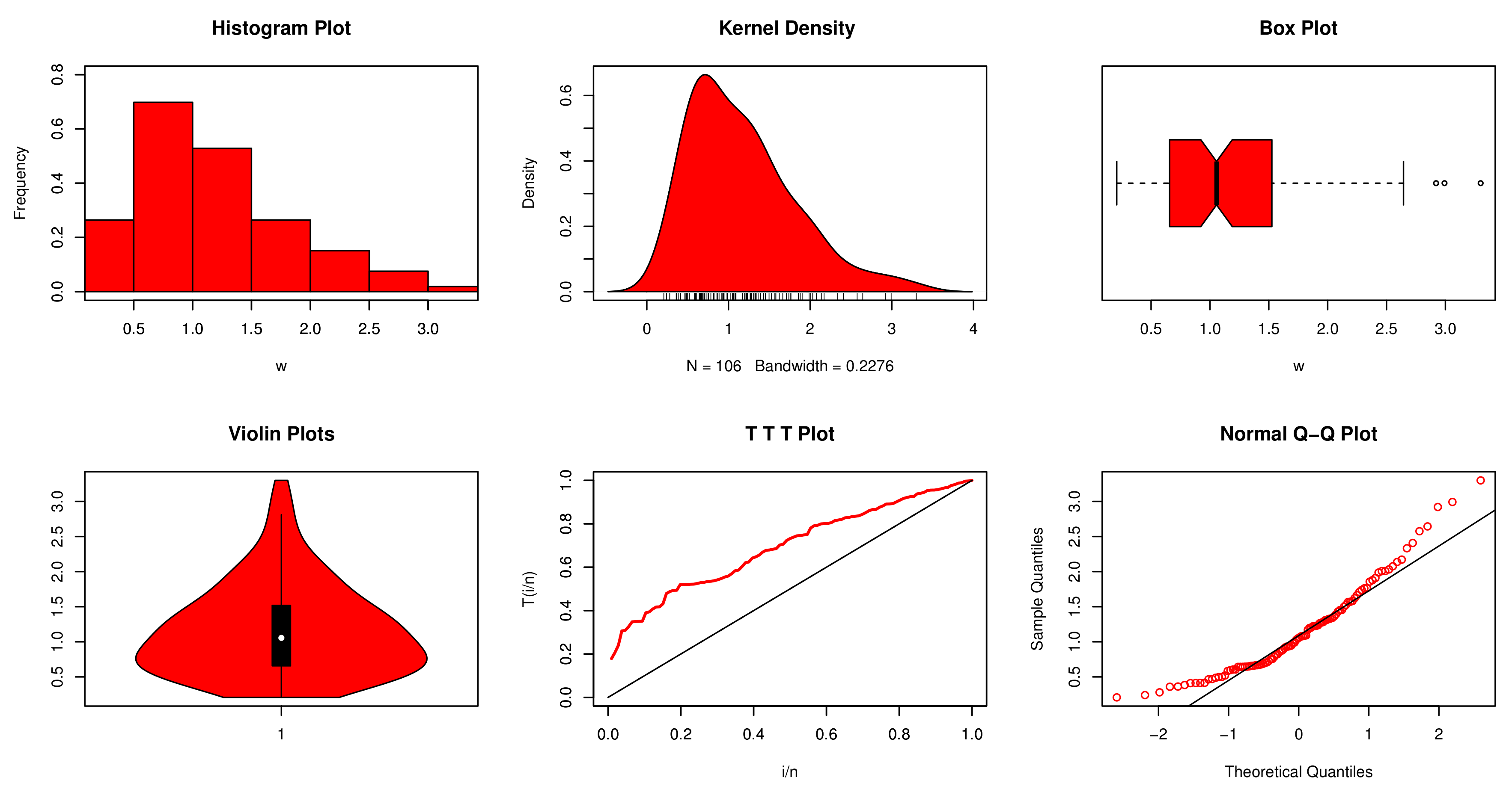
Corresponding to Data 1, the initial density shape is reported using the non-parametric kernel density estimation (KDE) approach in Figure 4, and it is noted that the density is asymmetric and unimodal. The normality condition is checked via the quantile–quantile (Q–Q) plot in Figure 4. The extremes are spotted using the box plot in Figure 4, and it is showed that some extreme observations were listed. Moreover, Figure 4 indicates that Data 1 has an increasing failure shape, based on the total time test (TTT) plot. For Data 2, the initial density shape, KDE, Q-Q plot, box plot, and TTT plot are presented in Figure 5. From the plots in Figure 5, we can see that the second dataset is unimodal, skewed to the right, and has an increasing failure shape.

Using the above mortality rate datasets, we show the applicability and best fitting capability of the NMFWE distribution. For this purpose, the comparison of the performance of the NMFWE distribution is made with the baseline FWE model, an exponentiated version of the FWE distribution, namely, an exponentiated FWE (E-FWE), the Weibull model, a generalization of the Weibull model, namely, the exponentiated Weibull (E-Weibull), and another famous extension of the Weibull model called the Kumaraswamy Weibull (K-Weibull) distribution. The SFs of the selected models are

• FWE:

  $$M(w;{\sigma }_1,{\sigma }_2)=e^{-e{\rm Y}(w;{\sigma }_1,{\sigma }_2)},w\ge 0,$$

  where ${\sigma }_1>0$ and ${\sigma }_2>0$;
• E-FWE:

  $$M(w;{\beta }_1,{\sigma }_1,{\sigma }_2)={\left(1-e^{-{\rm Y}(w;{\sigma }_1,{\sigma }_2)}\right)}^{{\beta }_1},w\ge 0,$$

  where ${\sigma }_1>0$, ${\sigma }_2>0$, and ${\beta }_1>0$;
• Weibull:

  $$M(w;{\sigma }_1,{\sigma }_2)=1-e^{-{\sigma }_2{w}^{{\sigma }_1}},w\ge 0,$$

  where ${\sigma }_1>0$ and ${\sigma }_2>0$;
• E-Weibull:

  $$M(w;{\beta }_1,{\sigma }_1,{\sigma }_2)={\left(1-e^{-{\sigma }_2{w}^{{\sigma }_1}}\right)}^{{\beta }_1},w\ge 0,$$

  where ${\sigma }_1>0$, ${\sigma }_2>0$, and ${\beta }_1>0$;
• K-Weibull:

  $$M(w;{\beta }_1,{\beta }_2,{\sigma }_1,{\sigma }_2)=1-{\left[1-{\left(1-e^{-{\sigma }_2{y}^{{\sigma }_1}}\right)}^{{\beta }_1}\right]}^{{\beta }_2},w\ge 0,$$

  where ${\sigma }_1>0$, ${\sigma }_2>0$, ${\beta }_1,$ and ${\beta }_2,>0$.

After choosing the competing models for comparative purposes, the very next step is to select the statistical tools to judge the performances of the fitted models. For the illustration and evaluation of these distributions, certain statistical tools and tests were selected and computed. These tools are given by

• AIC (Akaike information criterion), obtained as

  $$2k-2\delta \left(\lambda ,{\sigma }_1,{\sigma }_2|w_1,w_2,\cdots ,w_n\right);$$
• CAIC (corrected Akaike information criterion), calculated by

  $$\frac{2nk}{n-k-1}-2\delta \left(\lambda ,{\sigma }_1,{\sigma }_2|w_1,w_2,\cdots ,w_n\right);$$
• BIC (Bayesian information criterion), computed as

  $$klog\left(n\right)-2\delta \left(\lambda ,{\sigma }_1,{\sigma }_2|w_1,w_2,\cdots ,w_n\right);$$
• HQIC (Hannan–Quinn information criterion), obtained using the formula

  $$2klog\left(log\left(n\right)\right)-2\delta \left(\lambda ,{\sigma }_1,{\sigma }_2|w_1,w_2,\cdots ,w_n\right);$$
• AD (Anderson–Darling) test, having a mathematical expression given by

  $$-n-\frac{1}{n}\sum _{a=1}^n\left(2a-1\right)\left[logM\left(w_a\right)+log\left\{1-M\left(w_{n-a+1}\right)\right\}\right];$$
• CM (Cramér-von Mises) test, obtained using the formula

  $$\frac{1}{12n}+\sum _{a=1}^n{\left[\frac{2a-1}{2n}-M\left(w_a\right)\right]}^2;$$
• KS (Kolmogorov–Smirnov) test, whose value is computed using the expression

  $$su{p}_w\left[M_n\left(w\right)-M\left(w\right)\right].$$

From the expressions of the MLEs obtained in the previous section, we can observe that these expressions

$$\frac{\partial }{\partial {\sigma }_1}\delta \left(\lambda ,{\sigma }_1,{\sigma }_2|w_1,w_2,\cdots ,w_n\right),$$

$$\frac{\partial }{\partial {\sigma }_2}\delta \left(\lambda ,{\sigma }_1,{\sigma }_2|w_1,w_2,\cdots ,w_n\right),$$

and

$$\frac{\partial }{\partial \lambda }\delta \left(\lambda ,{\sigma }_1,{\sigma }_2|w_1,w_2,\cdots ,w_n\right),$$

are not in simple forms. Therefore, we have to adopt an optimization procedure to obtain the numerical values of $\widehat{{\sigma }_1},\widehat{{\sigma }_2}$, and $\widehat{\lambda }$.

For Data 1, the numerical values of $\widehat{{\sigma }_1},\widehat{{\sigma }_2},\widehat{\lambda },\widehat{{\beta }_1}$, and $\widehat{{\beta }_2}$ are presented in

Table 4. The numerical values of $\widehat{{\sigma }_1},\widehat{{\sigma }_2},\widehat{\lambda },\widehat{{\beta }_1}$, and $\widehat{{\beta }_2}$, using the first COVID-19 dataset.

Model	$\widehat{{\mathit{\sigma }}_1}$	$\widehat{{\mathit{\sigma }}_2}$	$\widehat{\mathit{\lambda }}$	$\widehat{{\mathit{\beta }}_1}$	$\widehat{{\mathit{\beta }}_2}$
NMFWE	0.61568 (0.06012)	1.33469 (0.20807)	2.86140 (1.76820)	-	-
FWE	0.64201 (0.05039)	1.11759 (0.10961)	-	-	-
E-FWE	0.65089 (0.11588)	1.35112 (2.14650)	-	0.82677 (1.39368)	-
Weibull	1.92159 (0.14090)	0.58694 (0.07121)	-	-	-
E-Weibull	1.00398 (0.32020)	1.78865 (0.75560)	-	4.02508 (3.10070)	-
K-Weibull	1.44294 (0.14370)	3.76192 (NaN)	-	3.13605 (1.63131)	0.24665 (NaN)

. The values of the comparative tools are provided in

Table 5. The values of AIC, CAIC, BIC, and HQIC of the fitted models, using the first COVID-19 dataset.

Model	AIC	CAIC	BIC	HQIC
NMFWE	186.12600	186.36130	194.11630	189.36450
FWE	189.04580	189.16230	196.37270	191.20480
E-FWE	187.01970	187.25500	195.01000	190.25820
Weibull	191.38590	191.50240	196.71280	193.54490
E-Weibull	188.2469 0	188.48220	196.23720	191.48540
K-Weibull	189.18680	189.58290	199.84060	193.50490

and

Table 6. The values of CM, AD and KS of the fitted models, using the first COVID-19 dataset.

Model	CM	AD	KS	p-Value
NMFWE	0.03276	0.20485	0.05085	0.94680
FWE	0.03963	0.26343	0.05313	0.92580
E-FWE	0.03866	0.25671	0.05589	0.89500
Weibull	0.10233	0.65790	0.06967	0.68220
E-Weibull	0.05380	0.29853	0.06758	0.71820
K-Weibull	0.04335	0.24179	0.06477	0.76540

. From the numerical illustrations of the fitted models in Table 5 and Table 6, we observe that the NMFWE model is the best one for modeling the mortality rate data. For the NMFWE distribution, the numerical values of the selected statistical measures are AIC = 186.12600, CAIC = 186.36130, BIC = 194.11630, HQIC = 189.36450, CM = 0.03276, AD = 0.20485, and KS = 0.05085, with p-value = 0.94680. Based on the KS criterion with the p-value, the FWE is the second-best model, with the respective values given by 0.05313 and 0.92580, whereas, by considering the AD and CM tools, the E-FWE is the best model. For the E-FWE model, these values are given by AD = 0.03866 and CM = 0.25671. From Table 5 and Table 6, it is now obvious that the NMFWE model is the best choice to apply for modeling the mortality rate data.

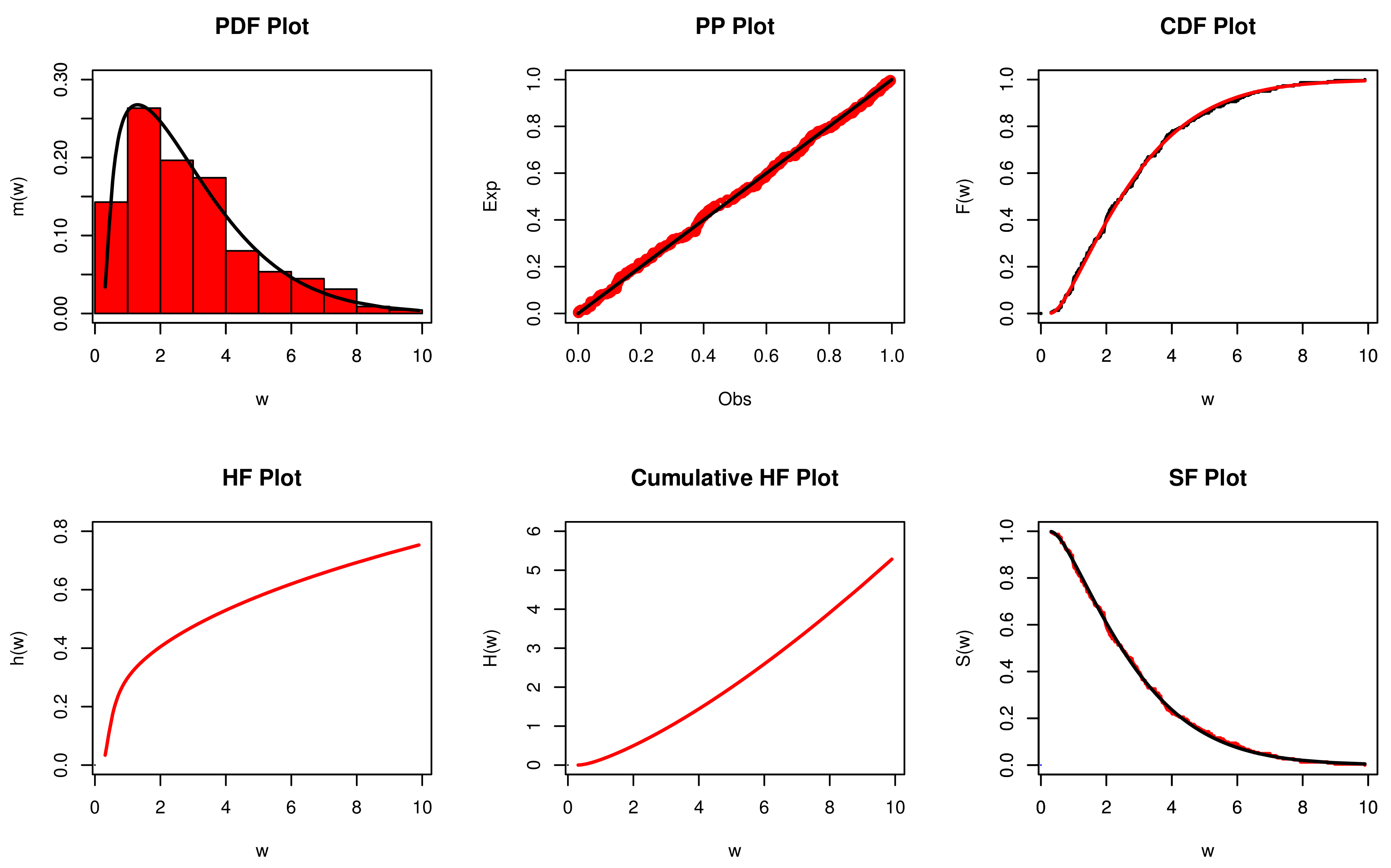
Furthermore, a visual illustration to support the numerical results is provided in Figure 6. For a visual illustration of the NMFWE distribution, the plots of the fitted PDF, PP, CDF, HF, CHF, and SF functions were obtained. These plots visually confirm the best fitting of the NMFWE distribution.

For Data 2, the numerical values of $\widehat{{\sigma }_1},\widehat{{\sigma }_2},\widehat{\lambda },\widehat{{\beta }_1}$, and $\widehat{{\beta }_2}$ are provided in

Table 7. The numerical values of $\widehat{{\sigma }_1},\widehat{{\sigma }_2},\widehat{\lambda },\widehat{{\beta }_1}$, and $\widehat{{\beta }_2}$, using the second COVID-19 dataset.

Model	$\widehat{{\mathit{\sigma }}_1}$	$\widehat{{\mathit{\sigma }}_2}$	$\widehat{\mathit{\lambda }}$	$\widehat{{\mathit{\beta }}_1}$	$\widehat{{\mathit{\beta }}_2}$
NMFWE	0.21080 (0.02141)	2.14767 (0.01293)	10.42059 (2.72864)	-	-
FWE	0.64201 (0.05039)	1.11759 (0.10961)	-	-	-
E-FWE	0.21612 (0.01809)	3.86071 (1.84962)	-	0.54707 (0.27101)	-
Weibull	1.61908 (0.08247)	0.14782 (0.02037)	-	-	-
E-Weibull	0.89210 (0.69863)	0.81533 (0.69098)	-	3.72610 (2.65132)	-
K-Weibull	1.20004 (NaN)	2.22247 (NaN)	-	4.63532 (0.13187)	0.14624 (0.01021)

. For this data, the values of the analytical tools are presented in

Table 8. The values of AIC, CAIC, BIC, and HQIC of the fitted models, using the second COVID-19 dataset.

Model	AIC	CAIC	BIC	HQIC
NMFWE	848.33910	848.44800	858.57400	852.47040
FWE	851.87659	851.90876	863.87654	856.75648
E-FWE	850.06480	850.17658	861.29978	854.19629
Weibull	859.51210	859.56640	866.33540	862.26630
E-Weibull	855.16730	855.27630	865.40220	859.29860
K-Weibull	852.71950	852.90220	866.36610	858.22800

and

Table 9. The values of CM, AD, and KS of the fitted models, using the second COVID-19 dataset.

Model	CM	AD	KS	p-Value
NMFWE	0.03762	0.21668	0.04217	0.82040
FWE	0.04076	0.25807	0.04746	0.71927
E-FWE	0.03975	0.24540	0.04819	0.67560
Weibull	0.13201	0.92260	0.05400	0.53080
E-Weibull	0.05951	0.40453	0.04895	0.65640
K-Weibull	0.04285	0.26641	0.04345	0.79130

. From the numerical comparison of the competing distributions in Table 8 and Table 9, we observe that the proposed NMFWE model is the best choice to implement for dealing with the mortality rate data. For the NMFWE distribution, the values of the analytical measures are AIC = 848.33910, CAIC = 848.44800, BIC = 858.57400, HQIC = 852.47040, CM = 0.03762, AD = 0.21668, and KS = 0.04217, with p-value = 0.82040. The second-best model, based on the KS test with p-value, is the K-Weibull distribution, with the respective values given by 0.04345 and 0.79130. By considering the other analytical tools, we observe that the E-FWE model is the second-best model.

To support the best fitting power of the NMFWE model, a visual illustration is provided in Figure 7. From the visual illustration in Figure 7, we can see that the NMFWE distribution follows the fitted PDF, CDF, and SF very closely.

Based on the obtained results in Table 4, Table 5, Table 6, Table 7, Table 8 and Table 9, we observe that the NMFWE model works quite well for analyzing the COVID-19 datasets. Therefore, it can be considered the best model among all competitive distributions, and we can utilize it as an alternative probability tool in prediction, rather than of recording data for a long period of time.

6. An Econometric Approach

In the previous section, the modified distribution is compared with numerous existing distributions under simulation and real data related to the mortality rate caused by the COVID-19 epidemic in Mexico and Canada. In this section, some pure statistical models are compared with machine learning algorithms via forecasting on the same datasets. The parametric autoregressive moving average (ARMA) and non-parametric autoregressive integrated moving average (NP-ARMA) are pure time series models, while neural network autoregression (NNAR) and support vector regression (SVR) are machine learning algorithms. Data splitting is needed to segment the data into two parts, in the form of training data and testing data, in order to obtain forecast errors. Therefore, 80 percent of the data is provided for model fitting, and 20 percent is preserved for the models’ comparison, following (Qi and Zhang, [29]). Details regarding each technique used for the modeling are given below.

6.1. The ARMA Model

In the time series forecasting literature, the ARMA is a powerful tool for univariate modeling. In the last few decades, ARMA has found successful applications in different areas such as economics, finance, engineering, and so forth (Khashei and Bijari, [30]). Generally, ARMA is a combination of autoregressive (AR) and moving average (MA) models. Mathematically, the ARMA can be written as

$${\pi }_t=\mu +\sum _{a=1}^m{\delta }_a{\pi }_{t-a}+\sum _{b=0}^n{\zeta }_b{\aleph }_{t-b},$$

(9)

where $\mu$ indicates an intercept term, ${\delta }_a(a=1,2,\cdots ,m)$ and ${\zeta }_b(b=1,2,\cdots ,m)$ represent the coefficients of AR and MA, respectively, and ${\aleph }_{t-b}$ represents the white noise term with zero mean and variance ${\sigma }_{\aleph }^2$. The order of m and n is often determined by an autocorrelation function (ACF) and by partial autocorrelation (PACF); see Bibi et al. [31]. In our case, we fit an ARMA (2, 1) model to the underlying time series ${\pi }_t$.

6.2. The NP-ARMA Method

The additive non-parametric counterpart of the ARMA process leads to an additive model (NP-ARMA), where the association between ${\pi }_t$ and its lagged variables do not have any specific known functional form. Probably, for any sort of non-linear form which is stated as

$${\pi }_t=g_1\left({\pi }_{t-1}\right)+g_2\left({\pi }_{t-2}\right)+,...,+g_k\left({\pi }_{t-m}\right)+{\aleph }_t,$$

(10)

where $g_i$$(i=1,2,\cdots ,k)$ show the smoothing functions which describe the association between ${\pi }_t$ and its own lagged variables, the functions $g_i$ represent the cubic regression splines (Shah et al., [32]). In the recent case, we incorporate four lags while estimating the model.

6.3. The NNAR Method

Customarily, a network or circuit of neurons leads to a neural network (NN). If the neurons or nodes are artificial, it leads to an artificial neural network. Neural network models have the potential to capture the complex non-linear nexus between an outcome variable and its covariates. A feedback NN is built with lagged time series variables as a covariate and hidden layer(s) with dimension nodes. NNAR consists of at least three layers of nodes: an output layer, a hidden layer, and an input layer. The outputs of a single layer are utilized as inputs to the succeeding one. A nonlinear NNAR model can be fitted/trained to predict a series by using its lagged variables as inputs ${\pi }_t,{\pi }_{t-1},\cdots ,{\pi }_{t-m}$; this process entails “so-called” feedback delays, where t represents the time delay parameter. The expression NNAR $(h,w)$ shows that there are h delay inputs and w nodes in the hidden layers. The NNAR is the same as ARMA $(h,0)$, conditionally, if there are zero nodes, i.e., NNAR $(h,0)$. However, here, the parameter which ensures stationarity is not incorporated (Bibi et al., [31]). The nonlinear NNAR equation can be expressed as

$${\pi }_t={\Omega }_0+\sum _{c=1}^h{\Omega }_c\zeta \left({\varphi }_c+\sum _{w=1}^z{\varphi }_{cw}{\pi }_{t-w}\right)+{\aleph }_t,$$

(11)

where ${\varphi }_c(c=1,2,\cdots ,h,w=1,2,\cdots ,z)$ and ${\Omega }_c(c=1,2,\cdots ,h)$ indicate the weights of interconnection, h shows the length of the hidden layers with activation function $\zeta$, and z shows the length of input layers. In our study, NNAR (6, 2) is utilized, which reveals six lagged variables, which are used as inputs, and two hidden layers. The input and hidden layers are selected for the model estimation through a trial-and-error approach, following (Khashei and Hajirahimi, [33]).

6.4. The SVR Method

Support vector regression is an alternative tool for solving regression issues such as nonlinearity and complexity in the data by introducing an alternative loss function (Vapnik et al. [34]; Vapnik [35]). SVR is based on the same principles as support vector machines (SVMs). It is an effective tool and has shown remarkable forecasting performance in many practical applications. The SVR utilizes different kernel functions to compute the resemblance between two data points to overcome the non-linearity. The core benefit of SVR lies in its capability to capture the covariate nonlinearity and then utilize it to boost the forecasting situations. It helps researchers discover a model’s acceptable margin of error (Bibi et al. [31]; Ribeiro et al. [36]). The mathematical form of SVR with kernel function can be described as

$${\pi }_t=\sum _{c=1}^h\left({\gamma }_c-{\gamma }_c^{*}\right)M\left(u_c,u\right)+\phi ,$$

(12)

where the kernel function $M\left(u_c,u\right)$ refers to the inner product, $\phi$ is adjusted within the kernel function, and ${\sum }_{c=1}^h\left({\gamma }_c-{\gamma }_c^{*}\right)$ is a constraint. Among numerous kernel functions, radial basis function (RBF) is commonly used, which can be described as

$$M\left(u_c,u\right)=exp\left(-\frac{\left|\right|u_c-u_m{\left|\right|}^2}{2{\sigma }^2}\right),$$

where $\left|\right|u_c-u_m{\left|\right|}^2$ represents the Euclidean distance amid the two covariate vectors squared and ${\sigma }_2$ shows the width of RBF (Lu et al., [37]). Our study proceeds with the RBF kernel function.

The predictive potential of all econometric models is evaluated by utilizing standard accuracy measures computed from a testing dataset. Statistically, the forecast errors are a more suitable criterion for assessing forecasting capability and for choosing the best tool. The widely used principles are mean absolute error (MAE), root mean square error (RMSE), and mean absolute percentage error (MAPE). Hence, our study adopts these three criteria to judge the models’ prediction performance. Their mathematical forms can be written as

$$MAE=mean\left(|{\pi }_t-\widehat{{\pi }_t}|\right),$$

$$RMSE=\sqrt{mean{\left({\pi }_t-\widehat{{\pi }_t}\right)}^2},$$

and

$$MAPE=mean\left(|\frac{{\pi }_t-\widehat{{\pi }_t}}{{\pi }_t}|\right)\times 100,$$

respectively.

6.5. Empirical Results

This section presents the findings of the forecasting experiments and some graphical representations. In this paper, we use the mortality rate of COVID-19 patients in Mexico and Canada, respectively, in order to quantify the predictability of the pure statistical and ML models. We split the data into two parts, intending to facilitate the out-of-sample prediction accuracy. For estimation, we use 80 percent of the data, and the remaining 20 percent of the data is used for checking the models’ multistep-ahead out-of-sample forecasting accuracy.

6.5.1. Analyzing the COVID-19 Data Taken from Mexico

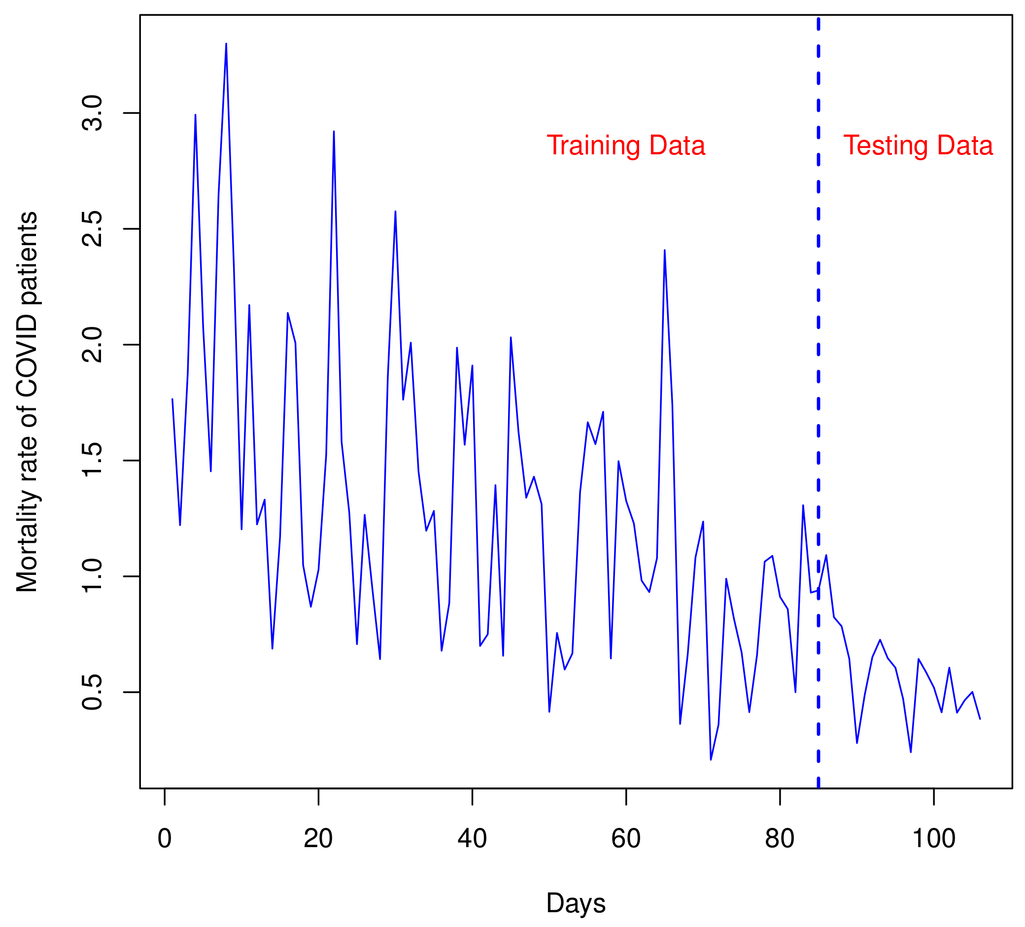
In Figure 8, the mortality rates of the COVID-19 patient data are divided by a vertical blue dotted line, where the training part is used for model estimation and the second part (testing data) is used for out-of-sample prediction.

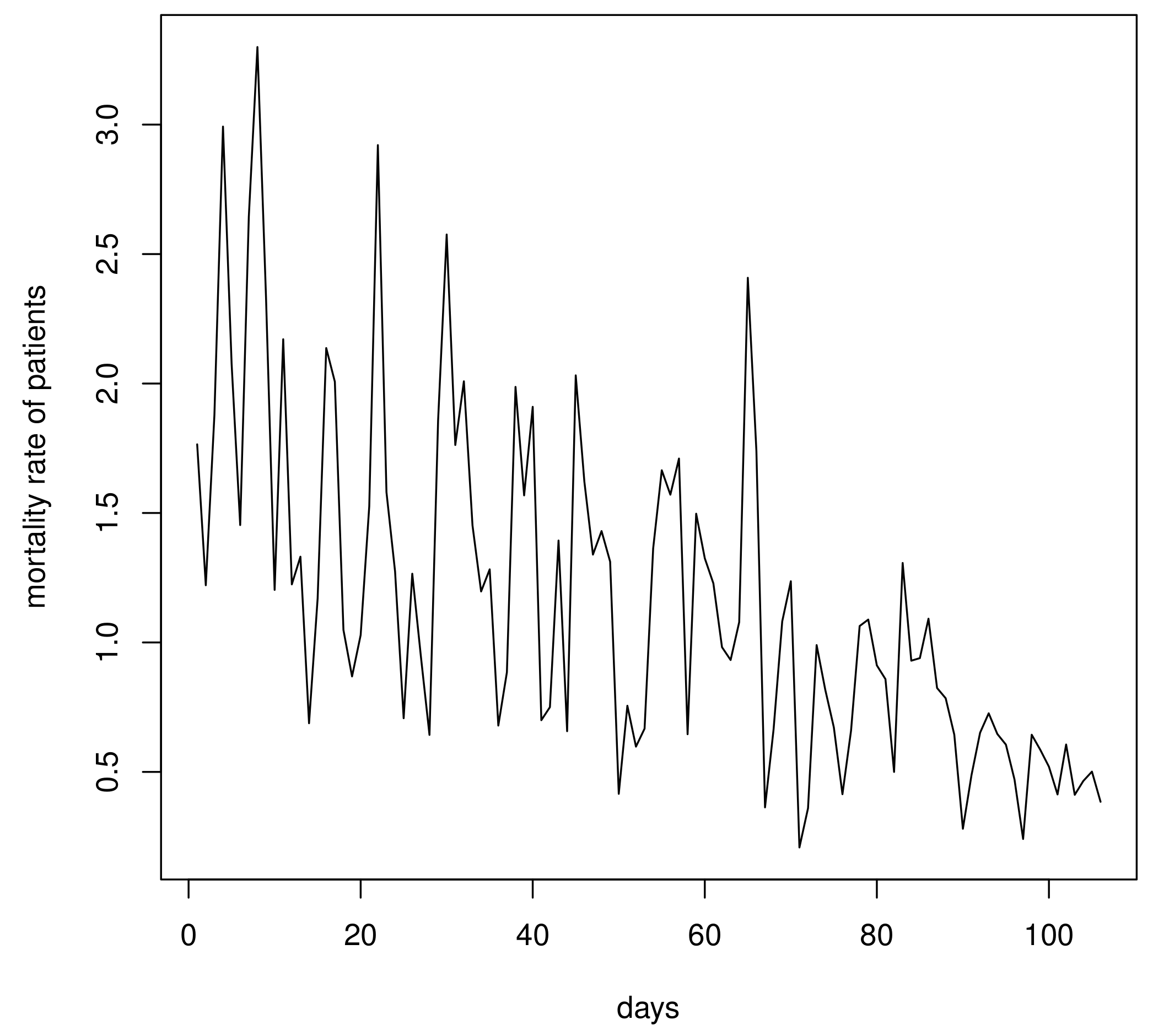
The data pattern in Figure 9 shows non-constancy in the mean, variance, and covariance over time, which provides a piece of evidence about the unit root problem. Similarly, ACF and PACF also illustrate that the original data of the mortality rates of COVID-19 patients is non-stationary; see Figure 10. In general, time series models such as ARMA require stationary series for modeling; thus, to achieve stationarity, we adopted a differencing approach. Post-differencing, ACF and PACF confirmed that the transformed series is stationary.

Table 10. The results of the Box–Ljung and Q-statistics tests.

Test	${\mathit{\chi }}^2$	p-Value
Box–Ljung test	23.697	0.10
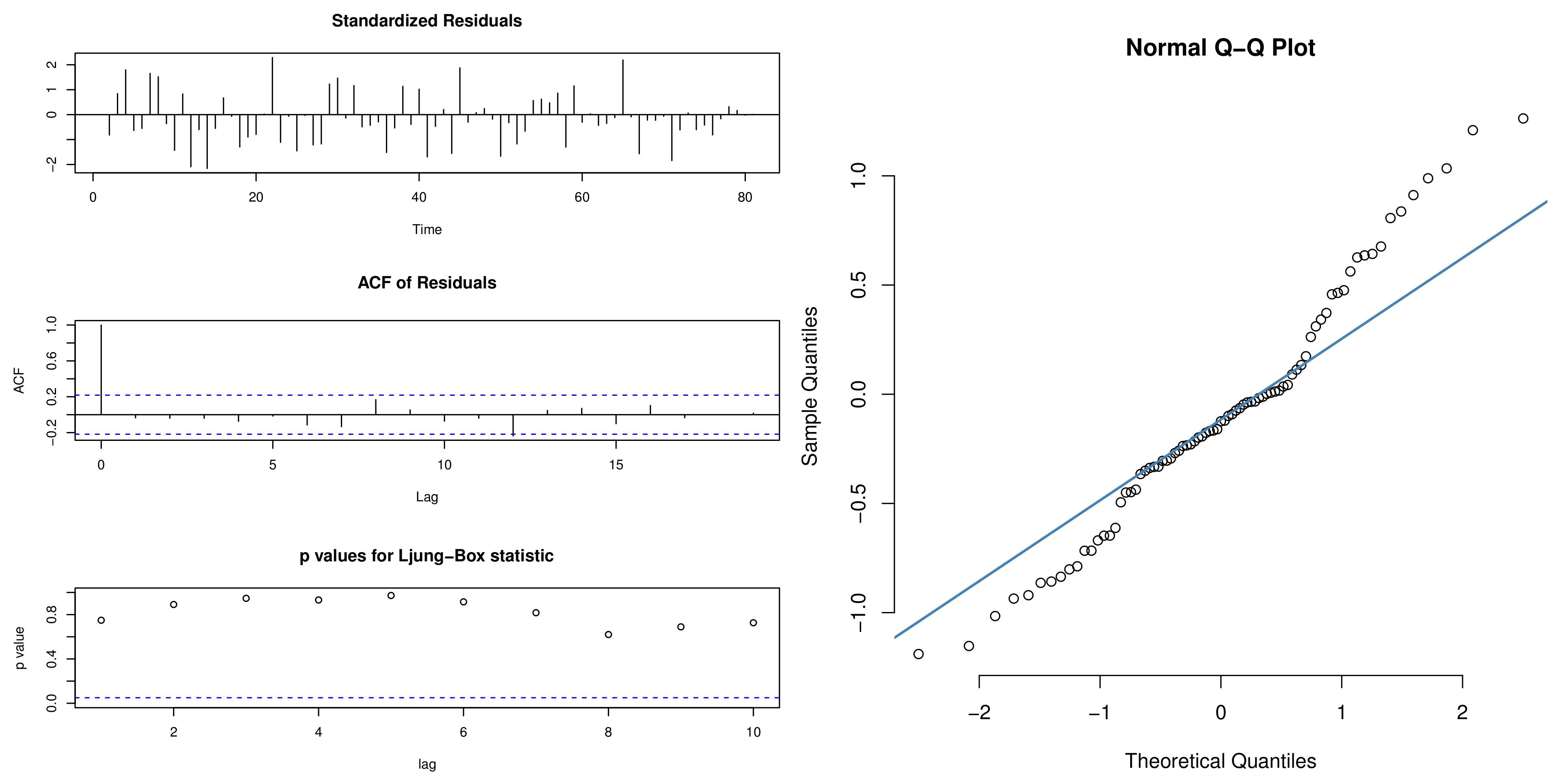
JB test	1.932	0.38

presents the results for the Jarque–Bera and Box–Ljung tests. The corresponding p-values exceed a five percent significance level; hence, we cannot reject the null hypothesis of random and normally distributed residuals of an estimated model. To be specific, it is declared that the residuals of the fitted model are uncorrelated and normally distributed. Thus, the ARMA model can be used for prediction.

Alternatively, to identify the normality and randomness of the fitted models’ residuals is to consider the graphs of the ACF, the Box–Ljung test, and the Q–Q plot of the residuals; see Figure 11. The plots in Figure 11 demonstrate that the residuals of the estimated model are random and normally distributed.

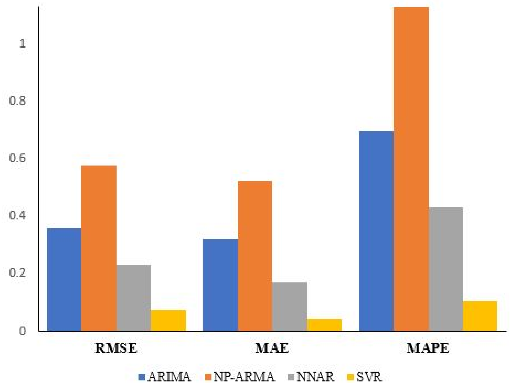
The three standard measures of accuracy under the COVID-19 dataset are reported in

Table 11. The error metrics using the COVID-19 dataset taken from Mexico.

Criteria	ARIMA	NP-ARMA	NNAR	SVR
RMSE	0.359	0.576	0.230	0.073
MAE	0.320	0.525	0.169	0.043
MAPE	0.696	1.127	0.431	0.104

. We can notice that RMSE, MAE, and MAPE computed for machine learning (ML) tools such as NNAR and SVR are substantially smaller than their pure statistical counterparts. Therefore, it can be concluded that predictions via ML tools tend to perform better than the rival statistical counterparts in terms of forecasting.

Furthermore, amid ML tools, the SVR outperforms the NNAR. A flowchart of forecast comparison is also presented in Figure 12. The plots in Figure 12 illustrate that ML tools, particularly SVR, remain effective tools for predicting the COVID-19 patient mortality rate trend. Moreover, Figure 13 also shows the performance of all models, and supports the output of Figure 12.

6.5.2. Analyzing the COVID-19 Data Taken from Canada

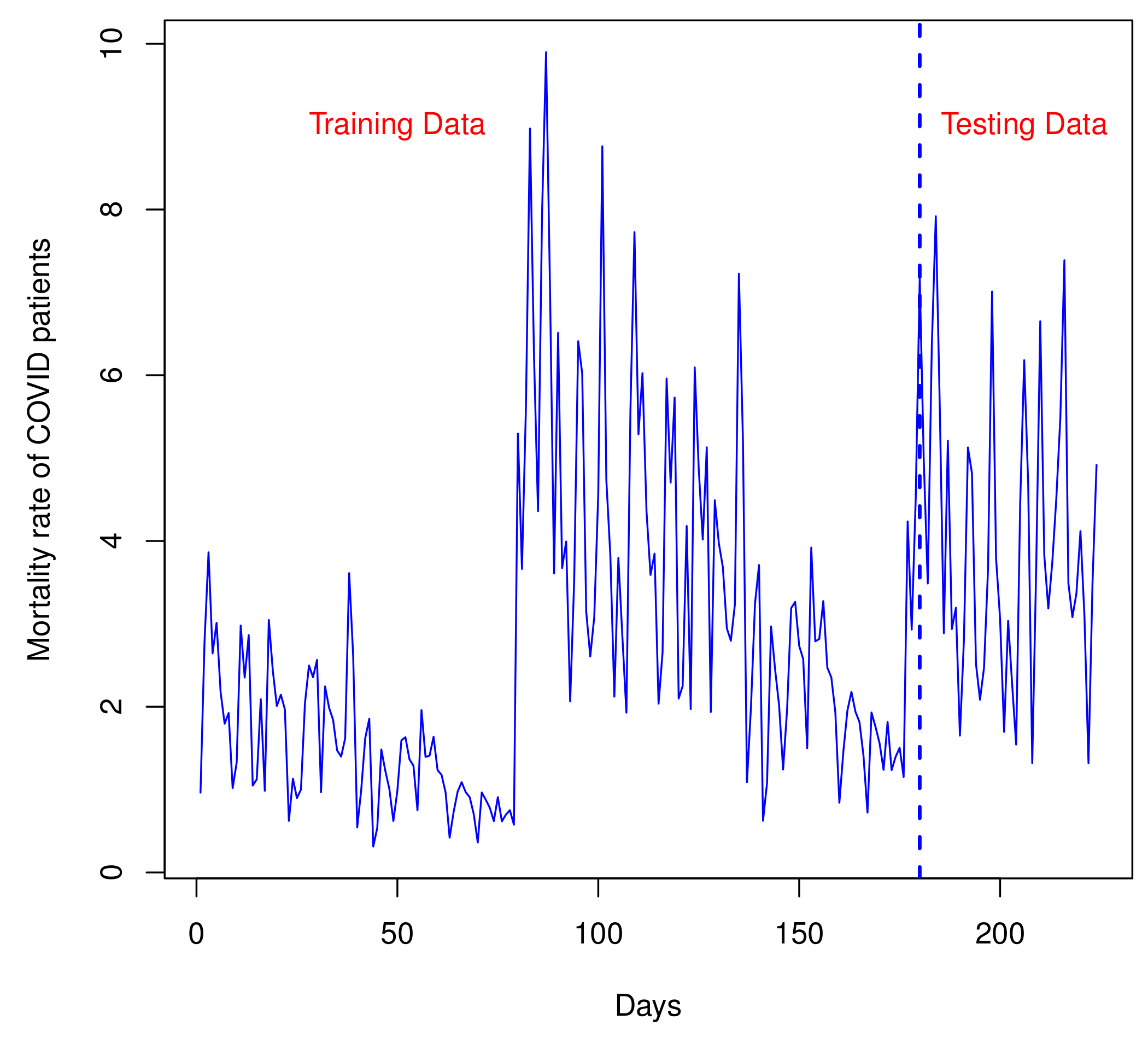
For estimating the models, we utilize 80 percent of the data, and the remaining 20 percent of the data is used for assessing the models’ multistep-ahead post-sample predictive power. In Figure 14, the mortality rate of the COVID-19 patients’ data is halved by a vertical blue dotted line, where the training part is utilized for model estimation and the second part (testing data) is utilized for post-sample forecasting.

The data pattern in Figure 14 shows non-constancy in the mean, variance, and covariance over time, which reflects the problem of a unit root. Likewise, the steady decline in the ACF plot reveals that the original data on the mortality rate of COVID-19 patients follow a random walk; see Figure 15. It is a fact that ARMA modeling requires stationary series; therefore, we take the first difference to make the underlying series stationary. Post-differencing, the ACF confirmed that the transformed series is stationary.

The numerical resutls of the Jarque–Bera and Box–Ljung tests are presented in

Table 12. The resutls of the Box–Ljung and Q-statistics tests.

Test	${\mathit{\chi }}^2$	p-Value
Box–Ljung test	17.95	0.59
JB test	0.172	0.91

. We can observe that the corresponding p-values exceed the five percent significance level; hence, we cannot reject the null hypothesis of random and normally distributed residuals. To be more specific, it is declared that the residuals of the fitted model are independent and follow a normal distribution. Therefore, the ARMA model can be used for prediction.

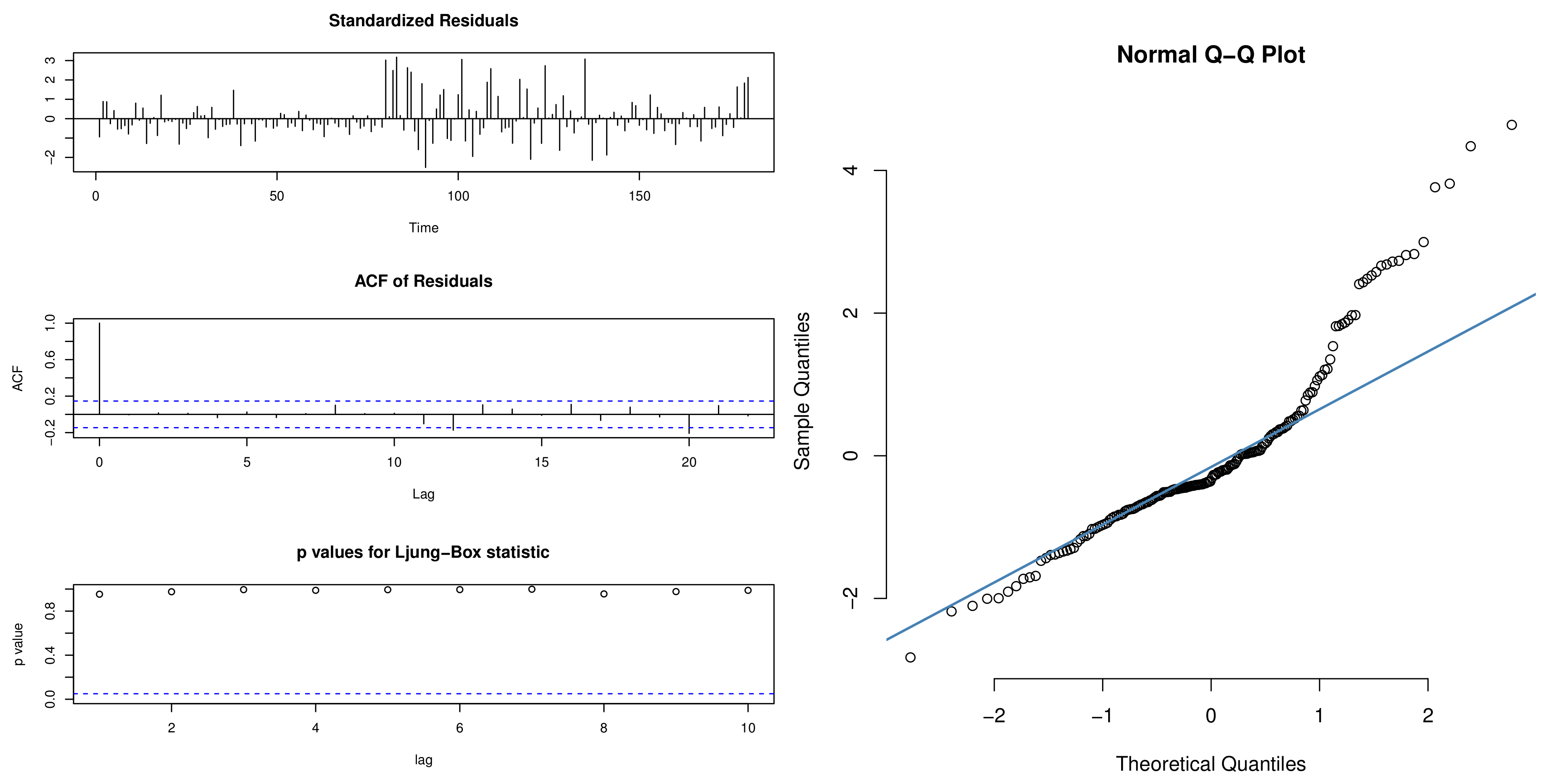
Alternatively, to identify the normality and randomness of the fitted models, we consider the graphs of the ACF, the Box–Ljung test, and the Q–Q plot of the residuals; see Figure 16. The plots in Figure 16 reveal that the residuals are random and normally distributed.

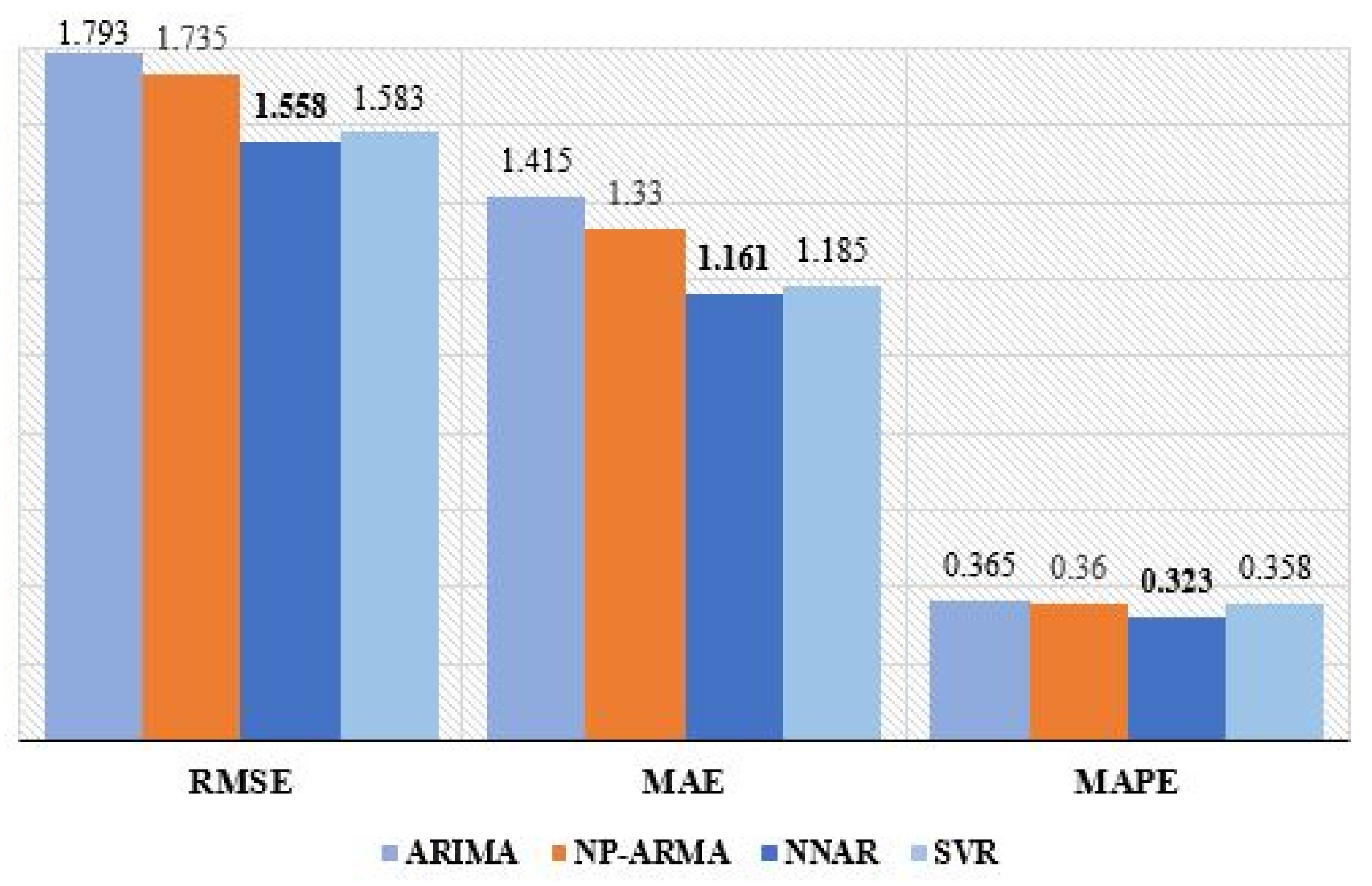
For the COVID-19 dataset of Canada, the same three standard measures of accuracy are reported in

Table 13. The error metrics.

Criteria	ARIMA	NP-ARMA	NNAR	SVR
RMSE	1.793	1.735	1.558	1.583
MAE	1.415	1.330	1.161	1.185
MAPE	0.365	0.360	0.323	0.358

. From the numerical results in Table 13, it is clear that the RMSE, MAE, and MAPE computed for the ML tools are substantially smaller. Hence, it can be inferred that predictions via the ML tools tend to perform better than their rival statistical counterparts in terms of forecasting. A flowchart of forecast comparison is also depicted in Figure 17.

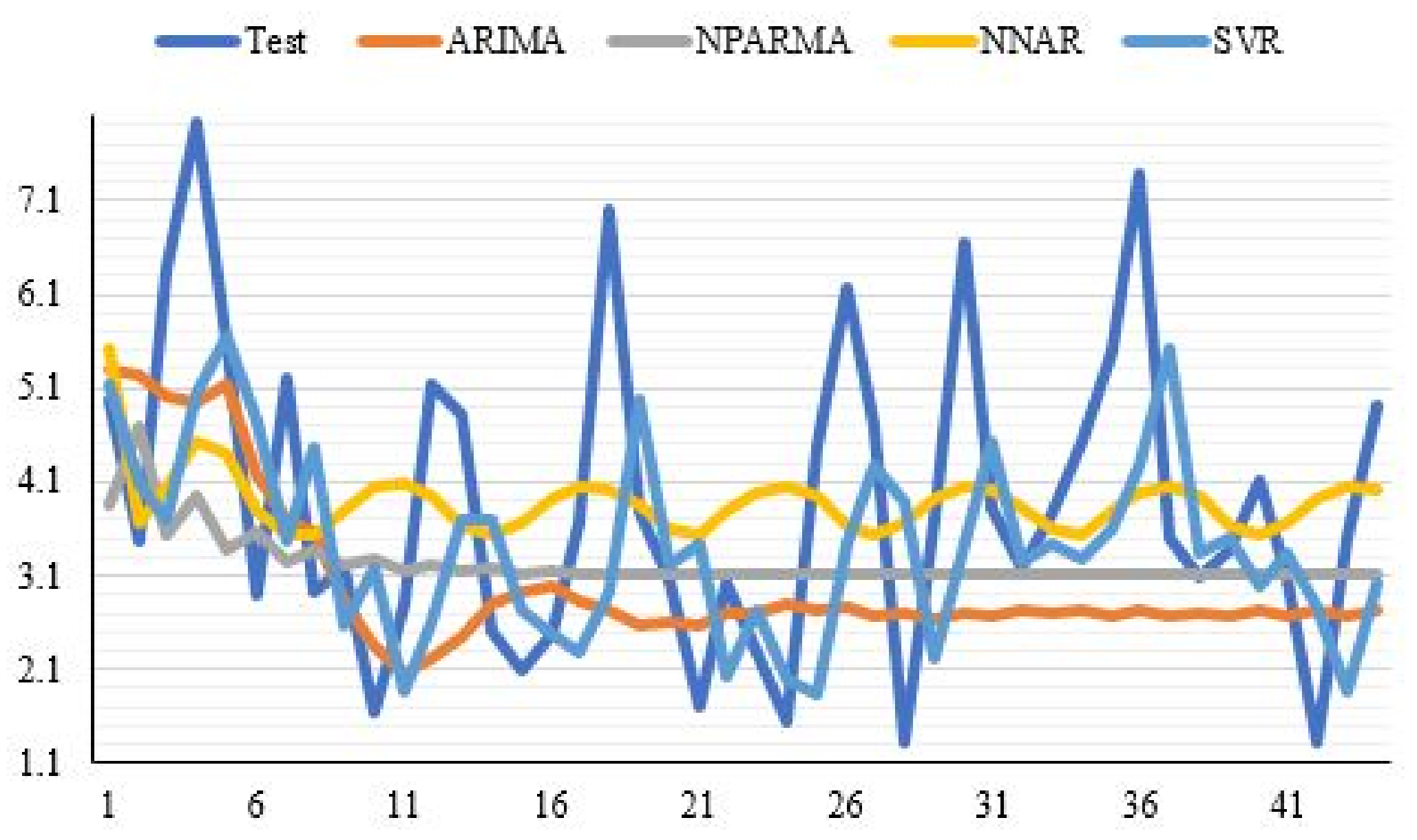
The plots in Figure 18 reveal that the ML algorithms, particularly NNAR, remain a more effective tool in capturing the pattern of the mortality rate of COVID-19 patients in Canada. In addition, Figure 18 also portrays the performance of all models and supports the output of Figure 17.

7. Final Remarks

The COVID-19 epidemic has highly affected the business, trade, education, economy, and health sectors, etc. Among the affected areas, the health sector is one of the most-affected sectors. To have the best description and knowledge of the COVID-19 epidemic, many statistical studies have been carried out. This paper has added some further contributions towards the literature on COVID-19 data modeling. This paper suggested a new statistical model for analyzing the mortality rate of the COVID-19 pandemic in Mexico and Canada. The new model was named the NMFWE distribution and was applied to COVID-19 data in comparison with other statistical models. Based on seven statistical quantities, it is observed that the NMFWE model was the best competitor for dealing with mortality rate data. In addition, the COVID-19 datasets were also modeled through pure statistical models including ARMA, NP-ARMA, and two ML algorithms, including NNAR and SVR. The RMSE, MAE, and MAPE are utilized to evaluate the effectiveness of the underlying models. The findings illustrate that ML algorithms are successful at predicting the mortality rate of COVID-19 patients. The results also suggested that SVR provides a better forecast than NNAR in the case of Mexico. On the other hand, in the case of Canada, the NNAR outperforms the SVR, showing clearly that increasing the number of observations improves the NNAR forecasting performance, as compared to SVR. In other words, it can be inferred that NNAR requires more data for accurate predictions, in contrast to SVR.

In the future, we are committed to employing the proposed model in the machine learning field. We are also motivated to introduce the bivariate extension of the proposed model for analyzing bivariate data in the health sector.

References

1. Hogan, C.A.; Sahoo, M.K.; Pinsky, B.A. Sample pooling as a strategy to detect community transmission of SARS-CoV-2. JAMA 2020, 323, 1967–1969. [Google Scholar] [CrossRef] [PubMed] [Green Version]
2. Mizumoto, K.; Kagaya, K.; Zarebski, A.; Chowell, G. Estimating the asymptomatic proportion of coronavirus disease 2019 (COVID-19) cases on board the Diamond Princess cruise ship, Yokohama, Japan, 2020. Eurosurveillance 2020, 10, 2000180. [Google Scholar] [CrossRef] [PubMed] [Green Version]
3. Ilyas, N.; Azuine, R.E.; Tamiz, A. COVID-19 pandemic in Pakistan. Int. J. Transl. Med. Res. Public Health 2020, 4, 37–49. [Google Scholar] [CrossRef]
4. Rao, G.S.; Aslam, M. Inspection plan for COVID-19 patients for Weibull distribution using repetitive sampling under indeterminacy. BMC Med. Res. Methodol. 2020, 21, 229. [Google Scholar] [CrossRef] [PubMed]
5. Singhal, A.; Singh, P.; Lall, B.; Joshi, S.D. Modeling and prediction of COVID-19 pandemic using Gaussian mixture model. Chaos Solitons Fractals 2020, 138, 110023. [Google Scholar] [CrossRef]
6. Qin, J.; You, C.; Lin, Q.; Hu, T.; Yu, S.; Zhou, X.H. Estimation of incubation period distribution of COVID-19 using disease onset forward time: A novel cross-sectional and forward follow-up study. Sci. Adv. 2020, 6, eabc1202. [Google Scholar] [CrossRef]
7. Almetwally, E.M.; Alharbi, R.; Alnagar, D.; Hafez, E.H. A new inverted topp-leone distribution: Applications to the COVID-19 mortality rate in two different countries. Axioms 2021, 10, 25. [Google Scholar] [CrossRef]
8. Almongy, H.M.; Almetwally, E.M.; Aljohani, H.M.; Alghamdi, A.S.; Hafez, E.H. A new extended Rayleigh distribution with applications of COVID-19 data. Results Phys. 2021, 23, 104012. [Google Scholar] [CrossRef]
9. Liu, X.; Ahmad, Z.; KKhosa, S.; Yusuf, M.; Alamri, O.A.; Emam, W. A New Flexible Statistical Model: Simulating and Modeling the Survival Times of COVID-19 Patients in China. Complexity 2021, 2021, 6915742. [Google Scholar] [CrossRef]
10. EL-Sagheer, R.M.; Eliwa, M.S.; Alqahtani, K.M.; EL-Morshedy, M. Asymmetric randomly censored mortality distribution: Bayesian framework and parametric bootstrap with application to COVID-19 data. J. Math. 2022, 2022, 8300753. [Google Scholar] [CrossRef]
11. Eliwa, M.S.; Altun, E.; El-Dawoody, M.; El-Morshedy, M. A new three-parameter discrete distribution with associated INAR (1) process and applications. IEEE Access 2020, 8, 91150–91162. [Google Scholar] [CrossRef]
12. El-Morshedy, M.; Eliwa, M.S.; Altun, E. Discrete Burr-Hatke distribution with properties, estimation methods and regression model. IEEE Access 2020, 8, 74359–74370. [Google Scholar] [CrossRef]
13. El-Morshedy, M.; Altun, E.; Eliwa, M.S. A new statistical approach to model the counts of novel coronavirus cases. Math. Sci. 2020, 16, 37–50. [Google Scholar] [CrossRef]
14. Altun, H.K.; Ermumcu, M.S.K.; Kurklu, N.S. Evaluation of dietary supplement, functional food and herbal medicine use by dietitians during the COVID-19 pandemic. Public Health Nutr. 2021, 24, 861–869. [Google Scholar] [CrossRef]
15. Altun, E.; El-Morshedy, M.; Eliwa, M.S. A new regression model for bounded response variable: An alternative to the beta and unit-Lindley regression models. PLoS ONE 2021, 16, e0245627. [Google Scholar]
16. Bebbington, M.; Lai, C.D.; Zitikis, R. A flexible Weibull extension. Reliab. Eng. Syst. Saf. 2007, 92, 719–726. [Google Scholar] [CrossRef]
17. El-Morshedy, M.; El-Bassiouny, A.H.; El-Gohary, A. Exponentiated inverse flexible Weibull extension distribution. J. Stat. Appl. Probab. 2017, 6, 169–183. [Google Scholar] [CrossRef]
18. El-Morshedy, M.; Eliwa, M.S.; El-Gohary, A.; Almetwally, E.M.; EL-Desokey, R. Exponentiated Generalized Inverse Flexible Weibull Distribution: Bayesian and Non-Bayesian Estimation Under Complete and Type II Censored Samples with Applications. Commun. Math. Stat. 2021, 1–22. [Google Scholar] [CrossRef]
19. Abubakari, A.G.; Kandza-Tadi, C.C.; Moyo, E. Modified Beta Inverse Flexible Weibull Extension Distribution. Ann. Data Sci. 2021, 7, 1–29. [Google Scholar] [CrossRef]
20. El-Gohary, A.; El-Bassiouny, A.H.; El-Morshedy, M. Exponentiated flexible Weibull extension distribution. Int. J. Math. Its Appl. 2015, 3, 1–12. [Google Scholar]
21. El-Damcese, M.A.; Mustafa, A.; El-Desouky, B.S.; Mustafa, M.E. The Kumaraswamy flexible Weibull extension. Int. J. Math. Its Appl. 2016, 4, 1–14. [Google Scholar]
22. Ahmad, Z.; Mahmoudi, E.; Dey, S. A new family of heavy tailed distributions with an application to the heavy tailed insurance loss data. Commun. Stat.-Simul. Comput. 2020, 49, 1–24. [Google Scholar] [CrossRef]
23. Gardiner, J.C.; Luo, Z.; Tang, X.; Ramamoorthi, R.V. Fitting heavy-tailed distributions to health care data by parametric and Bayesian methods. J. Stat. Theory Pract. 2014, 8, 619–652. [Google Scholar] [CrossRef]
24. Zhao, W.; Khosa, S.K.; Ahmad, Z.; Aslam, M.; Afify, A.Z. Type-I heavy tailed family with applications in medicine, engineering and insurance. PLoS ONE 2020, 15, e0237462. [Google Scholar] [CrossRef]
25. Bhati, D.; Ravi, S. On generalized log-Moyal distribution: A new heavy tailed size distribution. Insur. Math. Econ. 2018, 79, 247–259. [Google Scholar] [CrossRef]
26. Ahmad, Z.; Mahmoudi, E.; Hamedani, G.G.; Kharazmi, O. New methods to define heavy-tailed distributions with applications to insurance data. J. Taibah Univ. Sci. 2020, 14, 359–382. [Google Scholar] [CrossRef] [Green Version]
27. Ahmad, Z.; Mahmoudi, E.; Alizadeh, M.; Roozegar, R.; Afify, A.Z. The exponential TX family of distributions: Properties and an application to insurance data. J. Math. 2021, 2021, 3058170. [Google Scholar] [CrossRef]
28. Seneta, E. Karamata’s characterization theorem, feller and regular variation in probability theory. Publications de l’Institut Mathématique 2002, 71, 79–89. [Google Scholar] [CrossRef]
29. Qi, M.; Zhang, G.P. An investigation of model selection criteria for neural network time series forecasting. Eur. J. Oper. Res. 2001, 132, 666–680. [Google Scholar] [CrossRef]
30. Khashei, M.; Bijari, M. An artificial neural network (p, d, q) model for timeseries forecasting. Expert Syst. Appl. 2010, 37, 479–489. [Google Scholar] [CrossRef]
31. Bibi, N.; Shah, I.; Alsubie, A.; Ali, S.; Lone, S.A. Electricity Spot Prices Forecasting Based on Ensemble Learning. IEEE Access 2021, 9, 150984–150992. [Google Scholar] [CrossRef]
32. Shah, I.; Iftikhar, H.; Ali, S. Modeling and forecasting medium-term electricity consumption using component estimation technique. Forecasting 2020, 2, 163–179. [Google Scholar] [CrossRef]
33. Khashei, M.; Hajirahimi, Z. A comparative study of series arima/mlp hybrid models for stock price forecasting. Commun. Stat.-Simul. Comput. 2019, 48, 2625–2640. [Google Scholar] [CrossRef]
34. Vapnik, V.; Golowich, S.; Smola, A. Support vector method for function approximation, regression estimation and signal processing. In Advance in Neural Information Processing System; Mozer, M., Jordan, M., Petsche, T., Eds.; MIT Press: Cambridge, MA, USA, 1997; Volume 9, pp. 281–287. [Google Scholar]
35. Vapnik, V. Statistical Learning Theory; Wiley: New York, NY, USA, 1998. [Google Scholar]
36. Ribeiro MH, D.M.; da Silva, R.G.; Mariani, V.C.; dos Santos Coelho, L. Short-term forecasting COVID-19 cumulative confirmed cases: Perspectives for Brazil. Chaos Solitons Fractals 2020, 135, 109853. [Google Scholar] [CrossRef]
37. Lu, C.J.; Lee, T.S.; Chiu, C.C. Financial time series forecasting using independent component analysis and support vector regression. Decis. Support Syst. 2009, 47, 115–125. [Google Scholar] [CrossRef]
Figure 1. The PDF (left panel) and HRF (right panel) plots for the NMFWE distribution.
Mathematics 10 01792 g001
Figure 2. A visual display of the results of the SimS of the NMFWE model for σ 1 = 0.6 ,   σ 2 = 1.4 , and λ = 1.1 .
Mathematics 10 01792 g002
Figure 3. A visual display of the results of the SimS of the NMFWE model for σ 1 = 1.1 ,   σ 2 = 1.6 , and λ = 1.4 .
Mathematics 10 01792 g003aMathematics 10 01792 g003b
Figure 4. Nonparametric plots for Data 1.
Mathematics 10 01792 g004
Figure 5. Nonparametric plots for Data 2.
Mathematics 10 01792 g005
Figure 6. A visual illustration of the NMFWE model using Data 1.
Mathematics 10 01792 g006
Figure 7. A visual illustration of the NMFWE model using Data 2.
Mathematics 10 01792 g007
Figure 8. Divison of mortality rate of the COVID-19 patients data taken from Mexico.
Mathematics 10 01792 g008
Figure 9. Trend of mortality rate data taken from Mexico.
Mathematics 10 01792 g009
Figure 10. ACF and PACF for level (first row) and differenced data (second row).
Mathematics 10 01792 g010
Figure 11. Diagnostic check.
Mathematics 10 01792 g011
Figure 12. Forecasts comparsion for the COVID-19 dataset taken from Mexico.
Mathematics 10 01792 g012
Figure 13. Forecasting performance of the models.
Mathematics 10 01792 g013
Figure 14. The mortality rate of the COVID-19 patients in Canada.
Mathematics 10 01792 g014
Figure 15. ACF and PACF for level (first row) and differenced data (second row).
Mathematics 10 01792 g015
Figure 16. Diagnostic check.
Mathematics 10 01792 g016
Figure 17. Flowchart of forecast errors.
Mathematics 10 01792 g017
Figure 18. Forecasting performance of models.
Mathematics 10 01792 g018