Article

Growth Recovery and COVID-19 Pandemic Model: Comparative Analysis for Selected Emerging Economies

1
Institute of Complex Systems Mathematical Research, Moscow State University, 119991 Moscow, Russia
2
Mikhailovskaya Military Artillery Academy, 195009 St. Petersburg, Russia
3
Center for Fundamental Research, St. Petersburg State University of Economics, 191023 St. Petersburg, Russia
4
Engineering Faculty, Atlântica Instituto Universitário, 2730-036 Barcarena, Portugal
5
Keleti Károly Faculty of Business and Management, Óbuda University, 1084 Budapest, Hungary
6
Department of Finance, HSE University, 101000 St. Petersburg, Russia
*
Author to whom correspondence should be addressed.
Mathematics 2022, 10(19), 3654; https://doi.org/10.3390/math10193654
Submission received: 30 August 2022 / Revised: 26 September 2022 / Accepted: 30 September 2022 / Published: 5 October 2022

Abstract

:
The outburst of the COVID-19 pandemic and its rapid spread throughout the world in 2020 shed a new light on mathematic models describing the nature of epidemics. However, as the pandemic shocked economies to a much greater extent than earlier epidemics, the recovery potential of economies was emphasized and its inclusion in epidemic models is becoming more important. The present paper deals with the issues of modeling the recovery of economic systems that have undergone severe medical shocks, such as COVID-19. The proposed mathematical model considers the close relationship between the dynamics of pandemics and economic development. This distinguishes it from purely “medical” models, which are used exclusively to study the dynamics of the spread of the COVID-19 pandemic. Unlike standard SIR models, the present approach involves the introduction of the “vaccine” equation to the SIR model and introduces correction components that include the possibility of re-infection and other nuances such as the number of people at risk of infection (not sick with COVID but not vaccinated); sick with COVID; recovered; fully vaccinated (two doses) citizens; the rate of COVID infection; the rate of recovery of infected individuals; the vaccination coefficients, respectively, for those who have not been ill and recovered from COVID; the coefficient of revaccination; the COVID re-infection rate; and the population fluctuation coefficient, which takes into account the effect of population change as a result of births and deaths and due to the departure and return of citizens. The present model contains governance so that it not only generates scenario projections but also models specific governance measures as well to include the pandemic and restore economic growth. The model also adds management issues, so that it not only generates scenario forecasts but simultaneously models specific management measures as well, aiming to suppress the pandemic and restoring economic growth. The model was implemented on specific data on the dynamics of the spread of the COVID-19 pandemic in selected developing economies.

1. Introduction

Mathematical models describing the spread of the COVID-19 pandemic began to be developed almost simultaneously with the first outbreak in China in January 2020. These models are based on various approaches and aim to describe the continuous spread of COVID-19 adequately and accurately. Wang et al. [1] used a combination of a logistic model describing the rapid growth of the infected population and a model based on machine learning (FbProphet) to construct the epidemiological curve. Some other authors have proposed solutions based on the classical SIR-scheme models [2,3,4]. Finally, Contreras et al. [5] proposed a multi-group SEIRA model through populations with heterogeneous characteristics, taking into account the geographical features of the territory, behavioral features, and differences between social classes in a city, country, or region. However, an important feature of the COVID-19 pandemic is its systemic impact on the economy: temporary unemployment, the threat of bankruptcies, shocks in the anticipation of a decrease in production and demand, disruption of supply chains, and a sharp increase in sick pay [6,7,8]. All this forces change in economic policies and the development of mechanisms for an unprecedented amount of budget financing, including support for self-quarantine, as a means of flattening the epidemiological curve [9,10]. Another aspect of the impact of COVID-19 on the economy is the increasing income inequality through accumulating losses, mainly for workers with less education but not for those with an advanced degree [11]. In this regard, measures related to government support for specific segments of the economy, primarily employment systems, have been approved by the scientific community. For example, the EU’s decision to adopt “temporary support to reduce the risks of emergency unemployment” (SURE), under which up to 100 billion euros in loans to maintain employment, either in the form of short-term work (STW) or similar schemes, has been allocated to EU member states [12], or addressing specific economic challenges such as supply chain resilience (SCR) in manufacturing and service operations in sectors such as the automotive industry and air transportation. The recommendations in such studies boil down to a series of management decisions that include steps such as developing localized sources of supply and using advanced Industry 4.0 technologies for the automotive industry, the need to ensure business continuity based on the correct definition of operations both at airports and on the flights of the airlines themselves, or the widespread use of big data analytics (BDA) [13]. The tourism sector has become a separate object of research in terms of developing the necessary management decisions. Škare, Soriano, and Porada-Rochon [14] showed that the recovery of the global tourism industry will take longer than the average expected recovery period of 10 months, requiring the development of new risk management practices, including rethinking the impact of epidemics on the industry and coordination measures of private and public policy for the survival of the industry infrastructure during such crises.
A similar nature of the impact of a medical disease on the economy that consists of stimulating productive managerial decisions by the epidemic has not yet been seen in modern history. Devezas [15,16] characterizes COVID-19 as a “provocative” innovation that has the potential to trigger a profound global transformation, causing a sharp surge in digitalization, accelerated development of artificial intelligence, the dominance of remote forms of work, and an e-commerce boom. Furthermore, Stiglitz [17] draws conclusions about the inefficiency of traditional market mechanisms in the context of the global COVID-19 pandemic and points to the dependence of further economic growth on the active participation of governments in overcoming the pandemic and its consequences. These two features of the COVID-19 pandemic, which characterize its impact on economic development, are still insufficiently reflected in the existing mathematical models describing the spread of the pandemic.
In this paper, such an approach is proposed that allows the combination of purely medical aspects of COVID-19 such as vaccination for those who have not been sick or recovered from COVID, revaccination, re-infections with COVID, population fluctuations, etc., with its economic aspects, thus building cyclical forecasts and possible scenarios of pandemics.
Earlier research proved that the COVID-19 pandemic has influenced various aspects of business and daily life, including healthcare, economic, and social aspects of life [18]. Specifically, the economic consequences include the disruption of supply chains, slowing of manufacturing, and significant slowing down in revenue growth, which results in a decreasing GDP.
Various mathematical models have been developed to model the dynamics of the pandemic such as an updated SEIR model [19] that uses the ABC-fractional operator [20]. This model proposes a time-fractional model, and next to the four components of the SEIR model—the susceptible, exposed, infected, and recovered population—it splits the infected population into asymptomatic and symptomatic and considers the hospitalized population as well. The model uses the fixed point theory, claiming the existence and uniqueness of the solutions via this specific theory. The fractional-order model developed in [20] helps to analyze the dynamics of even a new virus, and the model results are claimed to be critical in understanding the dynamics of an epidemic.
The present model, which uses various theories, such as the abovementioned fixed point theory or chaos control, has novelty in its nature of linking the features and dynamics of pandemics, the effects of vaccination, and its potential effect on restoring economies. The novel modeling links the first, most widely used classic SIR Kermack–McKendrick model [21] and the Sanderson model [22,23] for the first time to describe the interaction between the pandemic, the economy, and the economic recovery.
The presented model contributes to the literature and the research field by combining an epidemiological and an economic model to trace the trajectories for economic recovery in which the level of people protected against COVID-19 reaches saturation.
Five emerging economies were selected to verify the presented model: India, Brazil, Indonesia, South Africa, and Kazakhstan. To a large extent, the choice was dictated by the desire to cover the geography as widely as possible, since COVID-19 spread very quickly across all continents. Secondly, developing economies could not allocate funds to fight the pandemic in such a volume as the developed economies of the world; it was the vaccination of the entire population and economic measures to support it in the face of severe restrictions on economic activity that made it possible to stabilize the epidemiological curve in different countries [24,25,26,27]. Thirdly, economies of different sizes and populations were chosen, allowing for different economic opportunities to deal with the pandemic. Finally, these countries have different health care systems and, accordingly, different potential opportunities to fight the pandemic and restore their economies.
This paper is structured as follows: after the theoretical framework, the model building, and definition, the related literature is discussed, and the data and model estimates are presented. This paper finishes with the conclusion section, including the discussion of the implications of the developed model.

2. Theoretical Framework and Mathematical Modeling

This work is devoted to the mathematical modeling of the processes of overcoming the pandemic and the restoration of economic growth, and modeling of the required volume of anti-crisis measures and the effective timing of their implementation. The section includes the related literature to support the theoretical framework and the mathematical modeling. As a basis for our modeling, the classic SIR Kermack–McKendrick model [21] and the Sanderson model [22,23] are proposed, which is used for the first time to link the interaction between the pandemic and the economy.

2.1. The Kermack–McKendrick Model

The Kermack-McKendrick model considers three groups of individuals: susceptible to the disease (Susceptible), infected (Infected), and recovered (Recovered). Transmission of infection occurs from infected individuals to susceptible individuals. The SIR model is described by a system of three differential equations:
{ d S d t = r S I d I d t = r S I v I d R d t = v I
where S(𝑡), 𝐼(𝑡), and 𝑅(𝑡) are the numbers of susceptible, infected, and recovering individuals at time t, respectively; 𝑟 is the rate of infection transmission; and ν is the rate of recovery of infected individuals.
Some experts consider it wrong to use SIR models to describe the coronavirus pandemic [28], but if appropriate changes are made, then such models can be used to describe the coronavirus pandemic. The main drawback of the SIR model is that it is not capable of generating scenarios for the periodic undulating spread of COVID-19. This disadvantage is eliminated by the modification carried out in this paper. The possibility of such a modification was proved in [29]. Thus, our work, based on statistical data on the coronavirus pandemic in Russia [30], contains monthly indicators of the incidence and recovery of Russian citizens during the coronavirus pandemic and shows that the dynamics of incidence and recovery has waves with peaks repeated with a frequency of 7 months. The proposed model adds a “vaccine” equation and transforms the differential equations to difference equations, thus creating an extended model. Zvyagintsev [29] has shown that such a model allows the generation of cyclic trajectories with the required periodicity, which is a period of 7 months in the present case. Verification of the periodic orbit with specific initial conditions based on the statistical data on COVID-19 for Russia was conducted in Sadovnichiy et al. [30]. The proposed model is then combined with the “Wonderland model” [22,23] and then, to overcome the chaotic dynamics and the random characteristics of morbidity and recovery, the modern theory of chaos control is used [31,32] and a controlling function is determined. Finally, the constructed system makes the modeling of the stabilization process possible both in order to overcome the pandemic and achieve economic recovery and support governmental and management decision-making processes.

2.2. The Wonderland Model

The discrete model proposed by Sanderson and Lutz [22,23] is called the “Wonderland model”. It models interrelated economic, demographic, and ecological processes and has the following form:
{ x j + 1 = x j ( 1 + β 0 ( β 1 e β y j 1 + e β y j ) α 0 ( α 1 e α y j 1 + e α y j ) ( α 2 ( 1 z j ) θ + 1 ) ) y j + 1 = y j ( 1 + γ ( γ + η ) ( 1 z j ) λ ) z j + 1 = z j e δ z j ρ ω x j y j p j 1 z j + z j e δ z j ρ ω x j y j p j   p j + 1 = ( 1 χ ) p j
where α 0 , α 1 , α 2 α , β 0 , β 1 , β , θ , γ , η , λ , δ , ρ , ω , χ , are positive constants; j = 0,1,2,…; x j is the population of a selected country x j 0 ; y j is the volume of GDP per capita; y j 0 ; z j is a numerical characteristic of the ecological level (quality of the environment)—natural capital 0 z j 1 ; and p j is a numerical characteristic of the degree of environmental pollution in the course of production, which is pollution per unit of production 0 p j 1 .
In the “Wonderland model”, the first equation defines the algorithm for the rate of population change in terms of the difference between birth and death rates. The second equation reflects the dynamics of the level of output per capita, taking into account the stock of natural capital. The third equation characterizes the quality of the environment and sets the growth of natural capital according to the logistic law. The fourth equation indicates the technological level of production and performs the function of controlling the intensity of environmental pollution.
In case of z j = 1 , it is believed that the ecology is in perfect condition and there is no environmental pollution at all. The case of z j = 0 expresses the opposite limiting case when environmental pollution is so great that there is a maximum threat to human health and the economy. For variable p j , the situation is the opposite. The value of p j = 1 corresponds to the highest degree of pollution per unit of production. If p j = 0 , then there is no pollution per unit of production, which indicates the highest technological level of production.

2.3. The Proposed Model

2.3.1. Extension of the SIR Model

In the SIR model (1), it is assumed that the recovered individuals acquire immunity and cannot be re-infected. For the COVID-19 pandemic, this assumption does not hold. In addition, model (1) does not take into account the process of vaccination against a viral infection. Let us add a “vaccine” equation to the SIR model and introduce correction components that consider the possibility of re-infection and other nuances. Equation (3) presents the extended model:
{ d S d t = r S I q S + a S d I d t = r S I v I + c R d R d t = v I c R + d V d V d t = q S d V + b R
where 𝑆(𝑡) is the number of people at risk of infection (not sick with COVID but not vaccinated), 𝐼(𝑡) is the number of people who are sick with COVID, 𝑅(𝑡) is the number of recovered, V(t) is the number of fully vaccinated (two doses) citizens; 𝑟 is the rate of COVID infection; ν is the rate of recovery of infected individuals; q and b are the vaccination coefficients for those who have not been ill and recovered from COVID, respectively; d is the coefficient of revaccination; c is the COVID re-infection rate; and a is the population fluctuation coefficient, which takes into account the effect of population change as a result of births and deaths and due to the departure and return of citizens.
According to Comunian et al. [28], SIR models do not fit to describe the coronavirus pandemic; however, with appropriate changes such as in Equation (3), modified models can be used to describe the coronavirus pandemic.
Since we operate with discrete values of coronavirus statistics, it is expedient for modeling to switch from differential equations to difference equations. Then, the epidemiological-mathematical model (3) is transformed into a discrete system of equations:
{ S j + 1 = S j ( 1 r I j q + a ) I j + 1 = I j ( 1 + r S j v ) + c R j R j + 1 = R j ( 1 c ) + v I j + d V j V j + 1 = V j ( 1 d ) + q S j + b R j
where j = 0,1,2,…, 𝑟 is the rate of COVID infection; ν is the rate of recovery of infected individuals; q and b are the vaccination coefficients for those who have not been ill and recovered from COVID, respectively; d is the coefficient of revaccination; c is the COVID re-infection rate; and a is the population fluctuation coefficient as a result of births and deaths and due to the migration of citizens. Actual coronavirus statistics are provided by official sources as specific discrete points in time. In this regard, in order to adapt the differential model (3) to actual realities, it is advisable to make the transition to a discrete model (4). Earlier, Zvyagintsev [26] showed that model (4) allows the generation of cyclic trajectories with the required periodicity. From the above, it follows that cycles with a period of 7 months are of interest. As a result of the computer experiment, the following numerical values of the system parameters (4) were selected:
r = 2.14970486321458; v = 1.80089137686731; q = 1.25507485843425;
α = 1.94597445654447; b = 0.0247039444045711;
c = 0.0619984179153856; d = 0.00807089279296773.
With the help of approximation methods, the following initial conditions were found under which the nonlinear system (4) models a periodic orbit with a period of 7 months:
S   ˜ 0 = 0.539753228690255 ;   I   ˜ 0 = 0.946101872256248 ; R   ˜ 0 = 2.23329875094284 ;   V   ˜ 0 = 3.89439991609052
.
These are the initial conditions, for which the solution of system (4) allows modeling of cyclical forecasts with a period of 7 in pandemic scenarios. These initial conditions (5) are universal for modeling 7-period cycles while the units of measurements are conditional individuals.
It should be noted that to find these 7-period cycles, it was necessary to calculate all the initial coordinates (5) up to the 14th decimal place, since the solutions of system (4) are very sensitive to changes in both the coefficients and the initial data. Furthermore, it should be noted that since real data are not always available for future forecasted time periods, the error cannot be established.
The periodic orbit modeled by system (4) with the initial conditions given in (5) based on the statistical data on COVID-19 for Russia was verified in Sadovnichiy, Akaev, Zvyagintsev, and Sarygulov [30]. In this case, the normalization coefficients B 1 , C 1 , B 2 , C 2 were chosen in such a way that the trajectories B 1 I   ˜ j + C 1 and B 2 R   ˜ j + C 2 fluctuated, respectively, from m i n I j to m a x I j and from m i n R j to m a x R j   . As a result of the calculations, the following was obtained:
B 1 = m a x I j m i n I j m a x I   ˜ j m i n I   ˜ j = 0.0024 ;   C 1 = m a x I j B 1   m a x I   ˜ j = 0.0036 B 2 = m a x R j m i n R j m a x R   ˜ j m i n R   ˜ j = 0.0021 ;   C 2 = m a x R j B 2   m a x R   ˜ j = 0.0046
Therefore, the formulae in (6):
I p r o g = 0.0024 I   ˜ j + 0.0036   and   R p r o g = 0.0021 R   ˜ j 0.0046
help to model COVID-19 predictive cycles that are adapted to epidemiological realities.
Since the solutions of system (4) are hypersensitive to changes in the initial data, then, due to the variation of the initial conditions, model (4) is able to simulate various scenarios that may well correspond to real epidemiological processes. As an example, let us take such initial conditions that are very close to the values in (5):
S 0 = 0.54 ;   I 0 = 0.95 ; R 0 = 2.23 ; V 0 = 3.89
.
By solving system (4) with the initial conditions in (7) and applying the normalization coefficients from (6), forecasts with a decreasing amplitude of fluctuations in the coronavirus epidemic can be made.
For the mathematical interpretation of the mutual influence of the pandemic and the economy, the equations from system (2) are used. Since every month the sum of susceptible (S), infected (I), recovered (R), and vaccinated (V) individuals is the total population of a country, then:
x j = S j + I j + R j + V j
holds.

2.3.2. Applying the “Wonderland Model”

Through z j , we denote the epidemiological level of infection with coronavirus, and p j is considered as an indicator of the effectiveness of medicine and healthcare in the fight against COVID. In the case of z j = 1 , it is considered that the epidemiological situation is in an ideal state and there is no infection with the coronavirus. The value z j = 0 expresses the opposite extreme case, where the size of the pandemic is so large that there is a maximum threat to human health and the economy. For p j , the situation is reversed. The value p j = 1 corresponds to a catastrophic case of the highest degree of coronavirus infection. If p j = 0 , then there is no COVID infection, which indicates a very high level of efficiency in medicine and healthcare.
The value of p j is calculated by the formula:
p j = I j x j
In the case of p j = 1 , the entire population is affected by the coronavirus I j = x j . If p j = 0 , there are no COVID patients I j = 0 . Then, the epidemiological situation is characterized by the equation (see the third equation in the “Wonderland model” (2)):
z j + 1 = z j e δ z j ρ ω y j I j 1 z j + z j e δ z j ρ ω y j I j
This equation defines a logistic law such that 0 z j + 1 1 . If, as a result of modeling, z j + 1 1 , the epidemiological situation improves, and the pandemic is overcome. If, as a result of modeling, z j + 1 0 , the epidemiological situation worsens, and the pandemic becomes catastrophic. The dynamics of an economy, taking into account the epidemiological situation, is reflected by the equation (see the second equation in model (2)):
y j + 1 = y j ( 1 + γ ( γ + η ) ( 1 z j ) λ )
where coefficients γ , η , λ , δ , ρ , ω are constants and y j is the volume of GDP per capita.
These equations demonstrate the dependence of an economy on the epidemiological situation. If, as a result of modeling, z j 1 , GDP is growing while, on the other hand, if, as a result of modeling, z j 0 , there is a decrease in GDP.
As a result, based on the aforementioned, the following mathematical model of the mutual influence of the pandemic and the economy is developed:
{ S j + 1 = S j ( 1 r I j q + a ) I j + 1 = I j ( 1 + r S j v ) + c R j R j + 1 = R j ( 1 c ) + v I j + d V j V j + 1 = V j ( 1 d ) + q S j + b R j z j + 1 = z j e δ z j ρ ω y j I j 1 z j + z j e δ z j ρ ω y j I j y j + 1 = y j ( 1 + γ ( γ + η ) ( 1 z j ) λ )
Governments are interested in overcoming the pandemic, restoring economic growth, and returning the socio-economic situation to a sustainable regime of a country. From a mathematical point of view, a stationary (fixed) point of system (8) corresponds to a stable regime. To find a fixed point, it is necessary to calculate such constants—S#, I#, R#, V#, z#, y# so that for all values of the indices j = 0,1,2,…, the identities Sj = S#, Ij = I#, Rj = R#, Vj = V#, zj = z#, yj = y# are performed. Therefore, it is necessary to find a solution to the algebraic system of equations:
{ S # ( 1 r I # q + a ) = S # I # ( 1 + r S # v ) + c R # = I # R # ( 1 c ) + v I # + d V # = R # V # ( 1 d ) + q S # + b R # = V # z # e δ z # ρ ω y # I # 1 z # + z # e δ z # ρ ω y # I # = z # y # ( 1 + γ ( γ + η ) ( 1 z # ) λ ) = y #
To find the coordinates of the fixed point of system (8), it is required to solve system (9). The solution of the algebraic system (9) has the form (10) and can be easily calculated by the standard method. The values from (10) are the coordinates of the fixed point of system (8). As a result of solving system (9), the fixed point coordinates for system (8) are the following:
S # = b v ( q a ) r ( a c b ( a q ) ) ; I # = a q r ;   R # = a v ( a q ) r ( a c b ( a q ) ) ;   V # = b v ( a q ) 2 d r ( a c b ( a q ) ) ; z # = 1 ( γ γ + η ) 1 λ ;   y # = δ r ω ( a q ) [ 1 ( γ γ + η ) 1 λ ] ρ .
Since the indicators of morbidity and recovery are characterized by randomness, in order to overcome the chaotic dynamics, model (8) is modified using the results from the modern theory of chaos control [28,29]. Let us introduce the notation:
w 1 ( j ) = S j ; w 2 ( j ) = I j ;   w 3 ( j ) = R j ; w 4 ( j ) = V j ; w 5 ( j ) = z j ;   w 6 ( j ) = y j
and rewrite system (8) in the vector form:
w ( j + 1 ) = F ( w ( j ) )   ; j   ϵ   { 0 ,   1 ,   2 ,   }
where:
( j ) = ( w 1 ( j ) w 2 ( j ) w 3 ( j ) w 4 ( j ) w 5 ( j ) w 6 ( j ) )   ;   F ( w ( j ) ) = ( w 1 ( j ) ( 1 r w 2 ( j ) q + a ) w 2 ( j ) ( 1 + r w 1 ( j ) v ) + c w 3 ( j ) w 3 ( j ) ( 1 c ) + v w 2 ( j ) + d w 4 ( j ) w 4 ( j ) ( 1 d ) + q w 1 ( j ) + b w 3 ( j ) w 5 ( j ) e δ w 5 ρ ( j ) ω · w 6 ( j ) w 2 ( j ) 1 w 5 ( j ) + w 5 ( j ) e δ w 5 ρ ( j ) ω · w 6 ( j ) w 2 ( j ) w 6 ( j ) ( 1 + γ ( γ + η ) ( 1 w 5 ( j ) ) λ ) )
For the vector function F, the Jacobi matrix has the following form:
A ( w ) = ( a 11 r w 2 0 q 0 0     r w 1 a 22 v 0 a 52 0     0 c 1 c b 0 0       0 0 d 1 d 0 0     0 0 0 0 a 55 a 65     0 0 0 0 a 56 a 66   )
where:
a 11 = 1 r w 2 q + a ,   a 22 = 1 + r w 1 v ,   a 66 = 1 + γ ( γ + η ) ( 1 w 5 ) λ , a 65 = λ ( γ + η ) w 6 ( 1 w 5 ) λ 1 ,   a 52 = ω w 6 w 5 ( w 5 1 ) e δ w 5 ρ ω · w 6 w 2 ( 1 w 5 + w 5 e δ w 5 ρ ω · w 6 w 2 ) 2 , a 55 = ( 1 + δ ρ ( 1 w 5 ) w 5 ρ ) e δ w 5 ρ ω · w 6 w 2 ( 1 w 5 + w 5 e δ w 5 ρ ω · w 6 w 2 ) 2 ,   and   a 56 = ω w 2 w 5 ( w 5 1 ) e δ w 5 ρ ω · w 6 w 2 ( 1 w 5 + w 5 e δ w 5 ρ ω · w 6 w 2 ) 2 .
After linearizing system (11) in the vicinity of the found fixed point w# with the coordinates w1# = S#, w2# = I#, w3# = R#, w4# = V#, w5# = z#, w6# = y#, we have:
w ( j + 1 ) = F ( w # ) F ( w ( j ) ) + A ( w # ) [ w ( j ) w # ] ,
Then, applying the Pyragas method [33], we obtain:
w ( j + 1 ) = F ( w # ) F ( w ( j ) ) + A ( w # ) [ w ( j ) w # ] + P ( j ) [ w ( j ) w ( j 1 ) ] ,
As a result, a modified system is achieved:
w ( j + 1 ) = F ( w ( j ) ) + U ( j )   ; j   ϵ   { 0 ,   1 ,   2 ,   } ,
where U(j) is a control function designed to stabilize the behavior of the system’s decisions. Based on the results of [28,29] on the stabilization of discrete systems, the control function of the following form is obtained:
U ( j ) = F ( w # ) F ( w ( j ) ) + A ( w # ) [ w ( j ) w # ] + P ( j ) [ w ( j ) w ( j 1 ) ] .
where P(j) is a periodic matrix of the following form:
( j ) = { ( k E A 2 ( w # ) ) ( A ( w # ) E ) 1 ,   j = 2 n O , j 2 n ,   n { 1 ,   2 ,   }   ,  
where 1 < k < 1 , E is the identity matrix, O is the zero matrix, A ( w # ) is the Jacobian matrix, and w # is the fixed point.
The discrete system (12) is characterized by ultra-high sensitivity to parameter changes. Even minor changes in the coefficients lead to significant changes in the behavior of the solutions. Thus, due to the variation of the coefficients, model (12) is able to simulate various scenarios that are quite consistent with real epidemiological and economic processes.
Governments are interested in overcoming the pandemic and restoring economic growth. The ideal scenario is considered to be the case when, thanks to the development of antiviral medicine and the implementation of mass vaccination, the incidence of coronavirus, and hence recovery, drops to zero. According to most medical experts, in order to develop herd immunity against coronavirus, it is necessary that the vaccinated proportion of the population is 70–80 percent. Israel’s positive experience shows that 100% vaccination is required to deal with the pandemic most effectively.
The derived Equations (12) and (13) are not only tools for efficient and adequate forecasting; the high efficiency is achieved as a result of finetuning of the model due to careful selection of the model parameters and their high-precision variation. A further advantage of this model is its ability to generate mathematically based management measures to stabilize socio-economic development in countries, which makes it possible to practically manage the dynamics of a pandemic and GDP. The constructed system (12) allows the modeling of the stabilization process due to the control function given in (13). The analytical Equation (13) obtained explicitly makes it possible to determine the size and time of proactive adjustments.

3. Data

Data from five emerging economies—Brazil, South Africa, Kazakhstan, India, and Indonesia—were collected and analyzed. The model considers each country independently. Data on incidence (Cases), the number of vaccinated (Vaccinations), mortality (Deaths), and recovered were taken from official websites [34,35] (https://ourworldindata.org/coronavirus (accessed on 27 August 2022)), https://www.worldometers.info/coronavirus/ (accessed on 5 May 2022)). The GDP forecast for 2022 was taken from the IMF review [36]. The number of employees and the dynamics of GDP in constant prices in 2015 were taken from the World Bank data (https://data.worldbank.org/indicator (accessed on 1 May 2022)) [37,38]. Data on investment (financial) multiples were used from the following sources [39,40,41].

4. Model-Based Estimates

Upon analyzing the epidemic waves and the virus variants, the highest peak of incidence fell on the Omicron strain, and the incidence dynamics had a “sawtooth” configuration. Figure 1 presents the daily rates of new coronavirus infections in the population of the selected countries during this period. The incidence dynamics has a clearly traceable cyclicity with a period of 7 days. Model (4) makes it possible to generate cyclic trajectories with the required frequency and configuration. As Figure 1 shows, the short-term cycles observed during the period of the Omicron strain are identical in these countries, and the frequency of these short-term cycles is 7 days for all the countries considered. Therefore, system (4) with the initial conditions given in (5) could be used again to model short-term cyclical forecasts during the period of the maximum COVID outbreak.
In order to model the forecast for overcoming the pandemic and developing an economy, the system defined in (12) with initial conditions that correspond to actual realities is solved. Table 1 shows the initial indicators computed based on official statistical data as of 30 June 2022, collected from the sources given in Section 3 [34,35,36,37,38,39,40,41]. Data in Table 1 are computed based on statistics from the official sources indicated in Section 3. Units of measurement are shares of the population of countries, rate between 0 and 1, and USD for GDP per capita.
Note that it is logical to assess the current level of overcoming the pandemic through vaccination and incidence rates. Therefore, it is assumed that:
z 0 = [ percentage   of   fully   vaccinated   population ] [ the   share   of   the   recovered   population ] .
The coefficients of the system (12) are tools for setting up the developed model (Table 2). Table 2 displays the numerical values of the parameters that were carefully selected for the model (12) and (13) as a result of a computer experiment. Since the numerical values of the parameters for the model were selected solely on the basis of statistical data from official sources, the experiment is fully consistent with the real data. The main criterion for compliance with real data was the full compliance with the actual indicators of the selected countries in terms of incidence, vaccination, and GDP per capita.
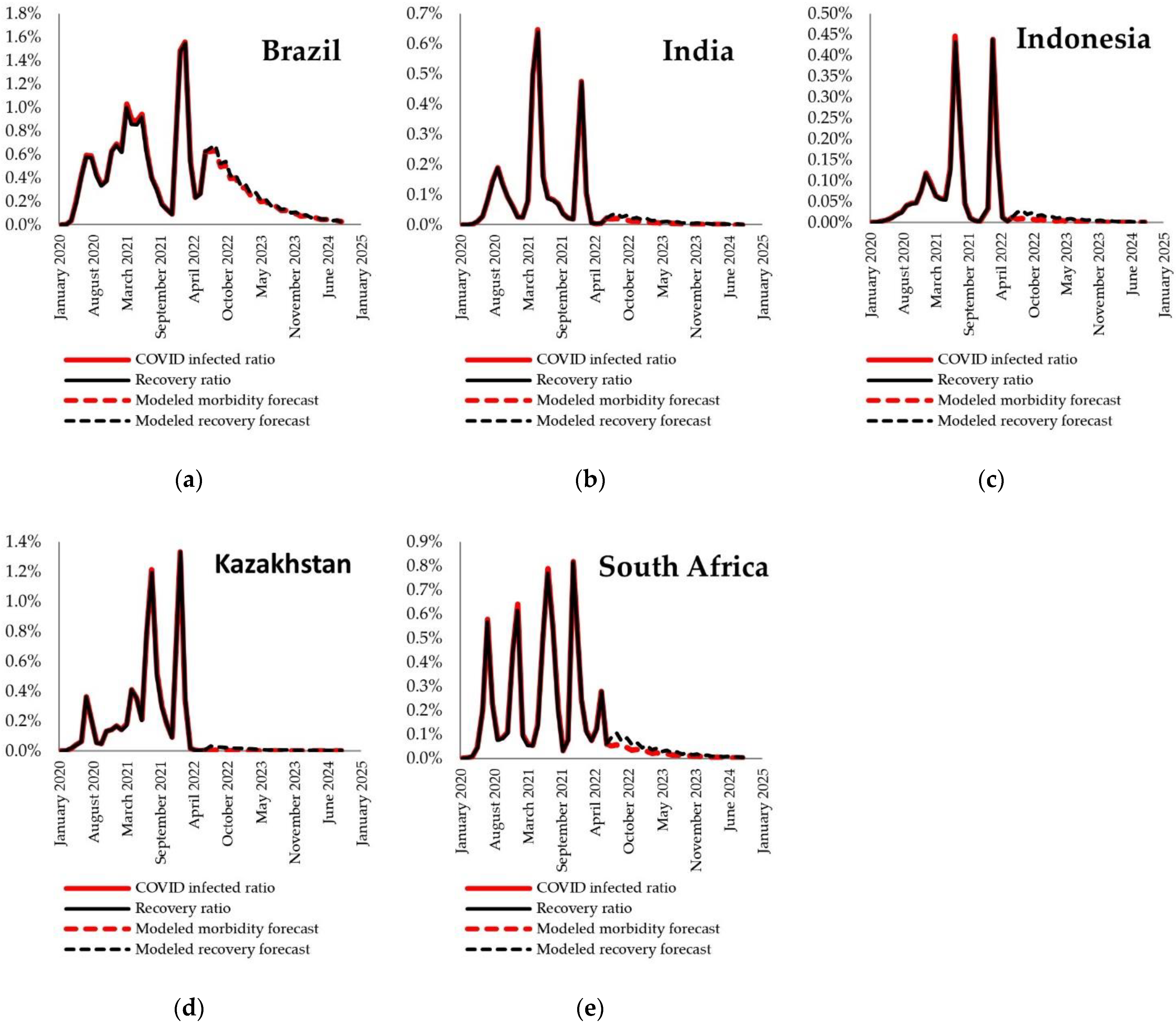
Having solved system (12) with the initial conditions from Table 1, the predictive trajectories of the pandemic in the selected countries, presented in Figure 2, Figure 3 and Figure 4, were obtained. Figure 2 clearly demonstrates that the countries under consideration have different medium-term cycles and different periodicities, it displays the COVID infected ratio, the recovery ratio, and the trajectories for the modeled morbidity and recovery ratios in Brazil, India, Indonesia, Kazakhstan, and South Africa.
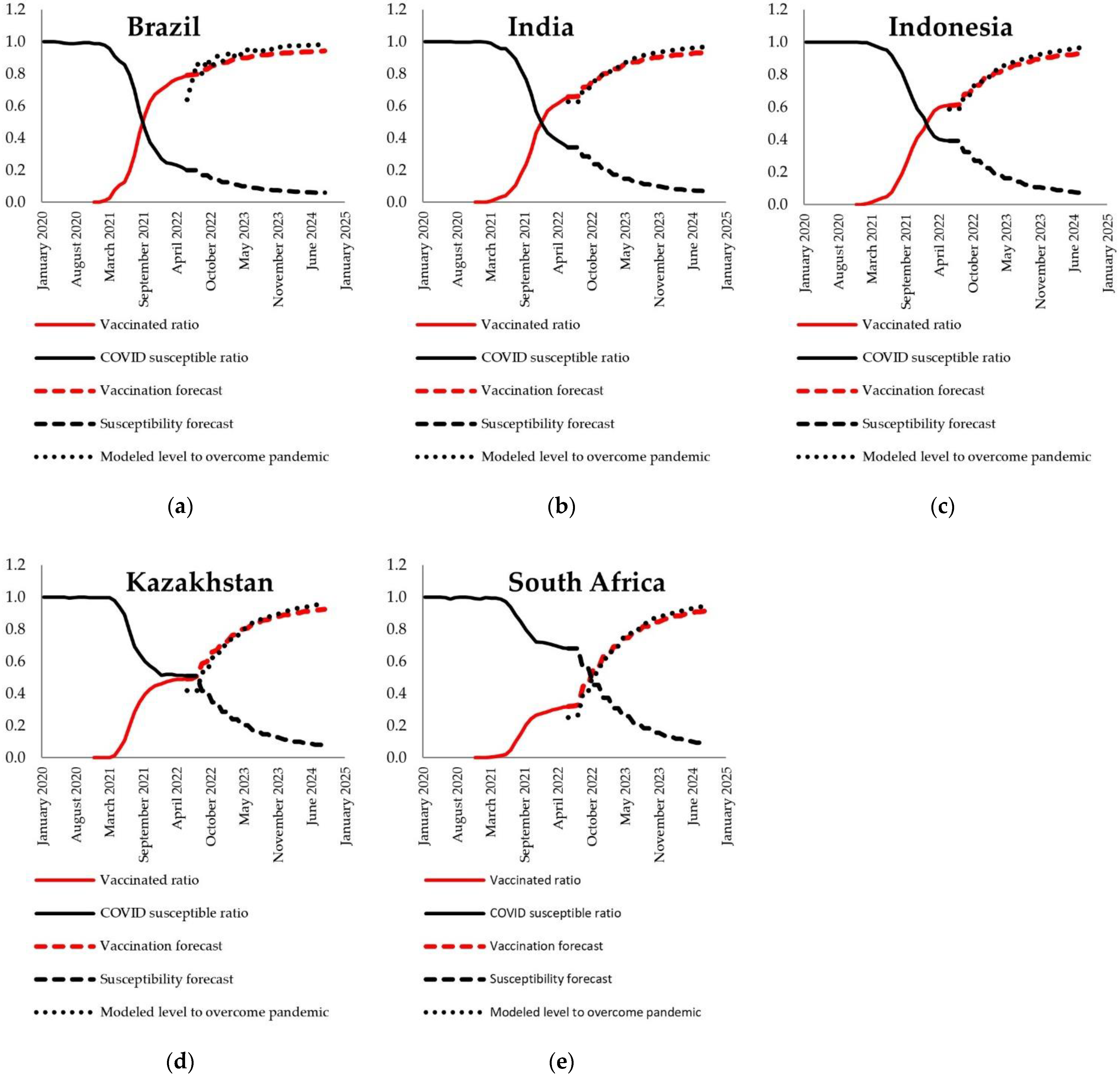
Figure 3 includes vaccination in the model and presents the vaccination and COVID susceptible ratios in the selected countries and the forecasts for vaccination, susceptibility, and, for each observed country, the modeled level to overcome the pandemic.
Figure 2 and Figure 3 clearly demonstrate that the vaccination of the population is the main tool in the fight against COVID-19, since the faster the population was vaccinated (slope of the curve of vaccinated ratio), the steeper the drop in the COVID susceptible ratio in each selected country (Figure 3). As the case of South Africa and Kazakhstan shown in Figure 3d,e, if vaccination stops, the rate of COVID susceptible stops decreasing and starts stagnating. Figure 3 shows that a higher vaccination rate results in a lower susceptible ratio and the trend of overcoming the pandemic shows a similar flattening, a slowing down tendency and converging to saturation level 1.
Figure 4 displays the modeled GDP per capita growth in the selected countries using systems (11) and (12), showing a definite recovery of economic growth even in countries experiencing a decreasing economic development trend. Figure 3 and Figure 4 assume a significant relationship between overcoming the pandemic and the recovery of economic growth; therefore, the correlation was checked between the vaccination rate and economic recovery. A strong positive correlation was found between the obtained values of w5(j) and w6(j), equaling 0.9, which proves this assumption. As a result of modeling, the values of these indicators show to stationary trajectories (Figure 3 and Figure 4). Since the indicators w 5 ( j ) = z j   and   w 6 ( j ) = y j were defined before Equation (11), the correlation coefficient is quite informative.
As a result of the calculations and the verification carried out on the basis of the results of the simulation, and taking into account investment multipliers, the monthly values for the scale of vaccination and the volume of additional investments necessary to overcome the pandemic and ensure economic growth—displayed in Table 3—were identified. The values are summarized in Table 3, presenting the results of calculations by Equations (12) and (13), which, in fact, is a schedule for the implementation of preventive anti-crisis measures.

5. Conclusions

Based on the results obtained, it can be concluded that in order to overcome the pandemic and restore economic growth, it is necessary to implement proactive corrective measures in a timely manner. The proposed model (12) and (13) can be used as an auxiliary tool for stabilizing socio-economic development. Equation (13) allows accurate calculation of the size of and time required for the necessary proactive adjustments. Thus, a toolkit was developed for modeling management measures aimed at suppressing the pandemic and ensuring economic growth.
The methods developed in this paper are quite convenient from a practical point of view and can be easily adapted to current realities. The discrete system (12) performs the function of simulation and generates various scenarios by varying the parameters. Model (12) with control (13) makes it possible to analyze the possibilities that contribute to bringing the socio-economic dynamics to a sustainable trajectory. The resulting model makes it possible to preliminarily estimate the size of managerial decisions aimed at preventing crisis tendencies. Upon using Equation (13), it is possible to calculate the exact size and time for the necessary impulse-like adjustments and model (12) and (13) can be useful in developing and implementing measures aimed at overcoming the pandemic and stabilizing economic development.
The proposed system of models in conceptual terms (1) takes into account the close relationship between the dynamics of the pandemic and economic development; (2) contains control features, thanks to which it not only generates scenario forecasts but forms specific management measures aimed at suppressing the pandemic and restoring economic growth as well; and (3) is a sixth-order discrete non-linear system, which more accurately reflects the nature of real statistical data that are formed at discrete times.
From a management point of view, the model allows the definition of a sequence of steps that includes (1) a preliminary assessment of the financial volumes necessary to prevent crisis tendencies; (2) calculation of the time and size of financial injections (impulse adjustments); and (3) assessment of opportunities that contribute to bringing the socio-economic dynamics to a sustainable trajectory.
As for the time horizons of the proposed model, it seems that its use is most effective in the initial phase of the spread of an epidemic, but it is not suitable for forecasting the epidemic itself. Subsequent studies will be aimed at improving the design scheme of the model.
The organization and implementation of management measures can only be carried out by government structures. Therefore, it is obvious that in a pandemic, the state should play a leading role in overcoming the crisis. Market mechanisms do not work during a pandemic. The market is not able to organize itself in such a way as to carry out preventive measures aimed at anticipating crisis phenomena. Using models (12) and (13), government agencies can analyze and estimate in advance the amount of financial and organizational costs required both to suppress the possible spread of an epidemic and ensure economic recovery. In accordance with the simulation results presented in this work, in the medium term, the priority tasks for governments are the implementation of vaccination and support of the economy in the required volumes and within a certain time frame.

Author Contributions

Conceptualization, A.A., A.I.Z. and A.S.; methodology, T.D.; software, A.T. and Y.I.; validation, A.I.Z.; formal analysis, T.D., A.T. and Y.I.; investigation, A.A. and A.S.; resources, A.T.; data curation, Y.I.; writing—original draft preparation, A.A.; writing—review and editing, T.D. and A.T.; visualization, A.I.Z.; supervision, A.S.; project administration, A.T., funding acquisition, A.T. All authors have read and agreed to the published version of the manuscript.

Funding

The research was supported by the Ministry of Science and Higher Education of the Russian Federation (Grant Agreement No. 075-15-2022-1136 dated 01.07.2022). The APC was partly funded by Óbuda University.

Institutional Review Board Statement

Not applicable.

Informed Consent Statement

Not applicable.

Data Availability Statement

There are no publicly archived datasets generated during the study.

Conflicts of Interest

The authors declare no conflict of interest.

References

  1. Wang, P.; Zheng, X.; Li, J.; Zhu, B. Prediction of epidemic trends in COVID-19 with logistic model and machine learning technics. Chaos Solitons Fractals 2020, 139, 110058. [Google Scholar] [CrossRef] [PubMed]
  2. Barlow, N.S.; Weinstein, S.J. Accurate closed-form solution of the SIR epidemic model. Phys. Nonlinear Phenom. 2020, 408, 132540. [Google Scholar] [CrossRef] [PubMed]
  3. Marinov, T.T.; Marinova, R.S. Dynamics of COVID-19 using inverse problem for coefficient identification in SIR epidemic models. Chaos Solitons Fractals X 2020, 5, 100041. [Google Scholar] [CrossRef]
  4. Nkwayep, C.H.; Contreras, S.; Tewa, J.J.; Kurths, J. Short-term forecasts of the COVID-19 pandemic: A study case of Cameroon. Chaos Solitons Fractals 2020, 140, 110106. [Google Scholar] [CrossRef] [PubMed]
  5. Contreras, S.; Villavicencio, H.A.; Medina-Ortiz, D.; Biron-Lattes, J.P.; Olivera-Nappa, Á. A multi-group SEIRA model for the spread of COVID-19 among heterogeneous populations. Chaos Solitons Fractals 2020, 136, 109925. [Google Scholar] [CrossRef] [PubMed]
  6. World Bank Group. Global Economic Prospects. January 2022; The World Bank Group: Washington, DC, USA, 2022; Available online: https://openknowledge.worldbank.org/bitstream/handle/10986/36519/9781464817601.pdf (accessed on 15 May 2022).
  7. International Labour Organization. ILO Monitor: COVID-19 and the World of Work. Seventh Edition. International Labour Organization, 2021. Available online: https://www.ilo.org/wcmsp5/groups/public/---dgreports/---dcomm/documents/briefingnote/wcms_767028.pdf (accessed on 5 May 2022).
  8. International Labour Office. World Social Protection Report 2020-22 Social Protection at the Crossroads—In Pursuit of a Better Future; International Labour Organisation (ILO): Genève, Switzerland, 2021. [Google Scholar]
  9. Baldwin, R. Keeping the Lights on: Economic Medicine for a Medical Shock. CEPR. Available online: https://cepr.org/voxeu/columns/keeping-lights-economic-medicine-medical-shock (accessed on 22 September 2021).
  10. Baldwin, R.E.; di Mauro, B.W. Economics in the Time of COVID-19; VoxEU.org eBook; CEPR Press: London, UK, 2020; Available online: https://www.sensiblepolicy.com/download/2020/2020_CEPR_McKibbin_Fernando_COVD-19.pdf (accessed on 5 May 2022).
  11. Furceri, D.; Loungani, P.; Ostry, J.D.; Pizzuto, P. COVID-19 Will Raise Inequality if Past Pandemics Are a Guide. CEPR. Available online: https://cepr.org/voxeu/columns/covid-19-will-raise-inequality-if-past-pandemics-are-guide (accessed on 11 September 2021).
  12. Balleer, A.; Gehrke, B.; Hochmuth, B.; Merkl, C. Guidelines for Cost-Effective Use of SURE: Rule-Based Short-Time Work with Workers’ Consent and Aligned Replacement Rates. CEPR. Available online: https://cepr.org/voxeu/columns/guidelines-cost-effective-use-sure-rule-based-short-time-work-workers-consent-and (accessed on 1 September 2021).
  13. Belhadi, A.; Kamble, S.; Jabbour, C.J.C.; Gunasekaran, A.; Ndubisi, N.O.; Venkatesh, M. Manufacturing and service supply chain resilience to the COVID-19 outbreak: Lessons learned from the automobile and airline industries. Technol. Forecast. Soc. Change 2021, 163, 120447. [Google Scholar] [CrossRef]
  14. Škare, M.; Soriano, D.R.; Porada-Rochoń, M. Impact of COVID-19 on the travel and tourism industry. Technol. Forecast. Soc. Change 2021, 163, 120469. [Google Scholar] [CrossRef]
  15. Devezas, T. The struggle SARS-CoV-2 vs. homo sapiens–Why the earth stood still, and how will it keep moving on? Technol. Forecast. Soc. Change 2020, 160, 120264. [Google Scholar] [CrossRef]
  16. Devezas, T. Aeronautics and COVID-19: A Reciprocal Cause-and-Effect Phenomenon. J. Aerosp. Technol. Manag. 2020, 12, e3420. [Google Scholar] [CrossRef]
  17. Stiglitz, J.E. The proper role of government in the market economy: The case of the post-COVID recovery. J. Gov. Econ. 2021, 1, 100004. [Google Scholar] [CrossRef]
  18. Haleem, A.; Javaid, M.; Vaishya, R. Effects of COVID-19 pandemic in daily life. Curr. Med. Res. Pract. 2020, 10, 78–79. [Google Scholar] [CrossRef] [PubMed]
  19. Li, M.Y.; Muldowney, J.S. Global stability for the SEIR model in epidemiology. Math. Biosci. 1995, 125, 155–164. [Google Scholar] [CrossRef]
  20. Sintunavarat, W.; Turab, A. Mathematical analysis of an extended SEIR model of COVID-19 using the ABC-fractional operator. Math. Comput. Simul. 2022, 198, 65–84. [Google Scholar] [CrossRef] [PubMed]
  21. Kermack, W.O.; McKendrick, A.G. A contribution to the mathematical theory of epidemics. Proc. R. Soc. Lond. Ser. Contain. Pap. Math. Phys. Character 1927, 115, 700–721. [Google Scholar] [CrossRef] [Green Version]
  22. Sanderson, W.C. Simulation Models of Demographic, Economic, and Environmental Interactions. In Population—Development—Environment; Lutz, W., Ed.; Springer: Berlin/Heidelberg, Germany, 1994; pp. 33–71. [Google Scholar] [CrossRef]
  23. Lutz, W. (Ed.) Population—Development—Environment: Understanding their Interactions in Mauritius; Springer: Berlin/Heidelberg, Germany, 1994. [Google Scholar] [CrossRef]
  24. Anderson, J.; Begamini, E.; Brekelmans, S.; Cameron, A.; Darvas, Z.; Domíngez Jiménez, M. The Fiscal Response to the Economic Fallout from the Coronavirus. Bruegel|The Brussels-Based Economic Think Tank. Available online: https://www.bruegel.org/publications/datasets/covid-national-dataset/ (accessed on 1 May 2022).
  25. RBK. The Accounts Chamber Estimated the Cost of Fighting the Pandemic, Cчeтнaя пaлaтa Oцeнилa вeличинy Pacxoдoв нa бopьбy c пaндeмиeй (In Russian). Available online: https://www.rbc.ru/economics/24/02/2021/6034d7659a7947b5e4403bdd (accessed on 1 May 2022).
  26. Asian Development Bank (ADB). Homepage|ADB COVID-19 Policy Database. 2020. Available online: https://covid19policy.adb.org/ (accessed on 12 May 2022).
  27. KPMG. Brazil—Government and Institution Measures in Response to COVID-19. 2020. Available online: https://home.kpmg/xx/en/home/insights/2020/04/brazil-government-and-institution-measures-in-response-to-covid.html (accessed on 1 May 2021).
  28. Comunian, A.; Gaburro, R.; Giudici, M. Inversion of a SIR-based model: A critical analysis about the application to COVID-19 epidemic. Phys. Nonlinear Phenom. 2020, 413, 132674. [Google Scholar] [CrossRef] [PubMed]
  29. Zvyagintsev, А.I. On a Nonlinear Differential System Modeling the Dynamics of the COVID-19 Pandemic, O HEЛИHEЙHOЙ ДИФФEPEHЦИAЛbHOЙ CИCTEME, MOДEЛИPYЮЩEЙ ДИHAMИKY ПAHДEMИИ COVID-19 (In Russian). Int. Res. J. Meждyнapoдный Hayчнo-Иccлeдoвameльcкuй Жypнaл 2022, 7, 116–121. [Google Scholar] [CrossRef]
  30. Sadovnichiy, V.A.; Akaev, A.A.; Zvyagintsev, A.I.; Sarygulov, A.I. Mathematical Modeling of Overcoming the COVID-19 Pandemic and Restoring Economic Growth. Dokl. Math. 2022, 106, 30–235. [Google Scholar] [CrossRef]
  31. Leonov, G.A.; Zvyagintseva, K.A. Piragas stabilization of discrete delayed feedback systems with a periodic pulse gain, Cтaбилизaция пo Пиpaгacy диcкpeтныx cиcтeм зaпaздывaющeй oбpaтнoй cвязью c пepиoдичecким импyльcным кoэффициeнтoм ycилeния (In Russian). Vestn. St. Petersburg Univ. Math. 2015, 48, 147–156. [Google Scholar] [CrossRef]
  32. Leonov, G.A.; Zvyagintseva, K.A.; Kuznetsova, O.A. Pyragas stabilization of discrete systems via delayed feedback with periodic control gain. IFAC-Pap. 2016, 49, 56–61. [Google Scholar] [CrossRef]
  33. Pyragas, K. Continuous control of chaos by self-controlling feedback. Phys. Lett. A 1992, 170, 421–428. [Google Scholar] [CrossRef]
  34. Ritchie, H.; Mathieu, E.; Rodés-Guirao, L.; Appel, C.; Giattino, C.; Ortiz-Ospina, E.; Hasell, J.; Macdonald, B.; Beltekian, D.; Roser, M. Coronavirus Pandemic (COVID-19). Our World Data. 2020. Available online: https://ourworldindata.org/coronavirus (accessed on 27 August 2022).
  35. Our World in Data. COVID Live—Coronavirus Statistics—Worldometer. Coronavirus Pandemic (COVID-19). Available online: https://www.worldometers.info/coronavirus/ (accessed on 5 May 2022).
  36. International Monetary Fund. World Economic Outlook, April 2022: War Sets Back the Global Recovery; IMF: Washington, DC, USA, 2022; Available online: https://www.imf.org/en/Publications/WEO/Issues/2022/04/19/world-economic-outlook-april-2022 (accessed on 5 May 2022).
  37. World Bank. GDP (Constant 2015 US$)—India, Indonesia, Brazil, South Africa, Kazakhstan|Data. Available online: https://data.worldbank.org/indicator/NY.GDP.MKTP.KD?end=2020&locations=IN-ID-BR-ZA-KZ&start=2014 (accessed on 1 May 2022).
  38. World Bank. Population, Total—India, Indonesia, Brazil, South Africa, Kazakhstan | Data. The Worldbank. Available online: https://data.worldbank.org/indicator/SP.POP.TOTL?end=2020&locations=IN-ID-BR-ZA-KZ&start=2014 (accessed on 1 May 2022).
  39. Organization for Economic Cooperation and Development. Quarterly National Accounts. Available online: https://stats.oecd.org/Index.aspx?DataSetCode=QNA (accessed on 12 May 2022).
  40. Dime, R.; Ginting, E.; Zhuang, J. Estimating Fiscal Multipliers in Selected Asian Economies. ADB Econ. Work. Pap. Ser. 2021, 638, 1–32. [Google Scholar] [CrossRef]
  41. Raga, S. Fiscal Multipliers: A Review of Fiscal Stimulus Options and Impact on Developing Countries. IDRC. 2022. Available online: https://set.odi.org/fiscal-multipliers-a-review-of-fiscal-stimulus-options-and-impact-on-developing-countries/ (accessed on 5 May 2022).
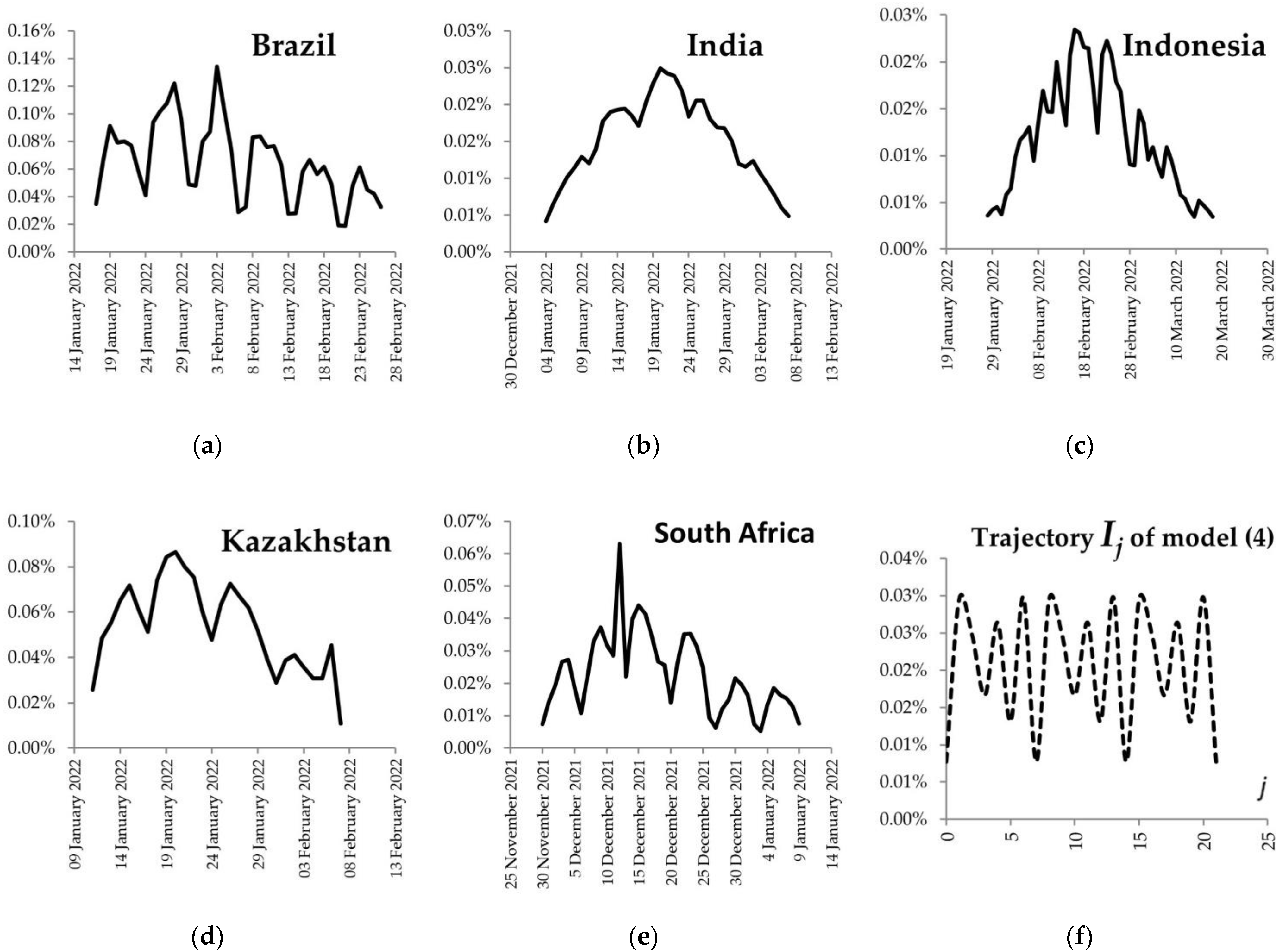
Figure 1. Infected proportion of the population and modeled 7-period morbidity trajectory of (a) Brazil, (b) India, (c) Indonesia, (d) Kazakhstan, (e) and South Africa, (f) trajectory Ij of model (4) (developed by authors).
Mathematics 10 03654 g001
Figure 2. Modeled forecasts of the dynamics of morbidity and recovery in (a) Brazil, (b) India, (c) Indonesia, (d) Kazakhstan, and (e) South Africa (developed by authors).
Mathematics 10 03654 g002
Figure 3. Modeled forecast of vaccination dynamics in (a) Brazil, (b) India, (c) Indonesia, (d) Kazakhstan, and (e) South Africa (developed by authors).
Mathematics 10 03654 g003
Figure 4. Modeled GDP per capita growth forecast in (a) Brazil, (b) India, (c) Indonesia, (d) Kazakhstan, and (e) South Africa (developed by authors).
Mathematics 10 03654 g004
Table 1. Initial data for system (12).
BrazilIndiaIndonesiaKazakhstanSouth Africa
w 1 ( 0 ) (Susceptible, %)0.1981180.3432690.3909490.5099770.68141
w 2 ( 0 ) (Infected, %)0.0062570.0002210.0001210.0000520.00059
w 3 ( 0 ) (Recovered, %)0.0062350.000220.000120.0000510.00058
w 4 ( 0 ) (Vaccinated, %)0.789390.656290.608810.489920.31742
w 5 ( 0 ) (Epidemiological level of infection)0.638180.62510.586780.416440.25091
w 6 ( 0 ) (GDP per capita, USD)8549.621953.943855.911269.45864.0
Table 2. Coefficients of the model (12) and (13).
BrazilIndiaIndonesiaKazakhstanSouth Africa
a0.0010.0010.0010.0010.001
b0.5510505
c0.30.30.30.30.3
d0.0000052631578950.0000052631578950.0000052631578950.0000052631578950.000005263157895
r1102010010
v0.350.81.35.30.8
q0.00110.00110.00110.00110.0011
γ0.000040.000040.000040.000040.00004
η0.40.40.40.40.4
λ22222
δ0.1904873858221330.004580024577144180.004475933109481820.002477376930364350.013011433457796
ω−0.2−0.2−0.2−0.2−0.2
ρ33333
k0.80.80.80.80.8
Table 3. Schedule of preventive anti-crisis measures.
Scale of Vaccination
(% of Country’s Population)
Additional Investments in the Economy
(bln USD)
DateBRAINDIDNKAZZAFBRAINDIDNKAZZAF
07.220.00.00.00.00.032.7021.7110.151.143.34
08.220.00.00.00.00.014.8021.5210.051.133.25
09.223.46.27.29.713.417.1235.6015.201.333.62
10.220.00.00.00.00.09.6314.166.600.732.11
11.222.75.05.87.810.713.1125.4610.730.902.42
12.220.00.00.00.00.06.259.264.310.471.37
01.232.24.04.66.28.610.1018.337.630.611.63
02.230.00.00.00.00.04.046.032.800.310.89
03.231.73.23.75.06.97.8313.295.460.411.10
04.230.00.00.00.00.02.613.911.820.200.57
05.231.42.53.04.05.56.109.733.940.280.74
06.230.00.00.00.00.01.682.531.170.130.37
07.231.12.02.43.24.44.777.192.880.200.51
08.230.00.00.00.00.01.081.630.760.080.24
09.230.91.61.92.63.53.755.362.120.140.35
10.230.00.00.00.00.00.691.050.490.050.15
11.230.71.31.52.02.82.954.041.580.100.24
12.230.00.00.00.00.00.450.680.310.030.10
01.240.61.01.21.62.22.333.071.190.070.17
02.240.00.00.00.00.00.290.440.200.020.06
03.240.50.81.01.31.81.852.350.900.050.12
04.240.00.00.00.00.00.180.280.130.010.04
05.240.40.70.81.01.41.471.810.690.040.09
06.240.00.00.00.00.00.120.180.080.010.03
07.240.30.50.60.81.11.171.400.530.030.06
08.240.00.00.00.00.00.080.120.050.010.02
09.240.20.40.50.70.90.931.090.410.020.05
Publisher’s Note: MDPI stays neutral with regard to jurisdictional claims in published maps and institutional affiliations.