Quantifying Intra-Catchment Streamflow Processes and Response to Climate Change within a Climatic Transitional Zone: A Case Study of Buffalo Catchment, Eastern Cape, South Africa

Abstract

The complexity of streamflow processes inhibits significant information about catchment performance and its sensitivity to climate change. Little is known about the severity of climate change within the coastal area of the monsoon–subtropical zone of climatic transition. This study advances a quasi-local scale analysis to simplify daily streamflow dynamics and their relationship with monthly hydro-climatic series (1981–2020) using six gauging stations on the Buffalo River due to its socio-economic significance. An integrated framework based on continuous wavelet transform (CWT), wavelet coherence (WC), innovative trend analysis (ITA), Mann–Kendall (MK), Sequential Mann–Kendall, and Pettitt tests were employed. CWT showed huge declivity in daily streamflow intensity (7676 to 719), >100 mm/day streamflow frequency (15 to 0), and wetness spell time-gap. WC obtained significant streamflow–rainfall co-movement of 8–196-month periodicities, which characterized Buffalo as anti-phase (1–4-month), lag-lead (8–32-month), and in-phase (64–196-month) in processes. The Buffalo River’s sensitivity to significantly decreasing rainfall trends and increasing temperature trends depicts Streamflow–ENSO teleconnection. Contrarily, ITA and MK exhibited significantly increasing trends of tributaries’ low flow and inferred the perennial status of the catchment. The Pettitt test corroborates the deductions and asserts 1990 (temperature), 1996 (streamflow), and 2004/2013 (rainfall) as the abrupt change points, while SMK captured a critical streamflow slump in 2015–2020. Overall, the study proved the reductionist approach and model framework to achieve the hydrological process simplification and resolution of hotspots of hydrologic extremes within a bimodal climate with complex topography. This study remarks on the management policy of the BR and provides a reference for managing water resources and catchment hydro-climatic extremes.

1. Introduction

Water provision in the Buffalo River Basin (BRB), a relatively small but significant basin to the Buffalo City Metropolitan Municipality, South Africa, is becoming a critical managerial issue due to the slump in dam water level [1,2,3]. The BRB depends mainly on a storage-limited inter-granular and fissure aquifer system that is recharged by a highly sporadic and bimodal rainfall-flow regime system [4,5,6,7]. The insufficient catchment hydrologic study on the BRB underpins the lack of uncertainty on the factors driving the streamflow variability. Particularly, the geolocation of the BRB within the transition zone of monsoon and subtropical climates means its streamflow is subjugated by the accentuated impact of climate change from two dissimilar zones [4,6,7]. Regional studies on the interannual variability of hydro-climates and the impact of climate change have predicted more frequent and intense hydrologic extremes inducing streamflow variability, however, with uncertainty on its impact at a reduced scale [6,7,8].

Hydrologic extremes of floods and drought are costly natural disasters due to their impact on sustainable development. The United Nations Office for Disaster Risk Reduction [9] reported that the global loss of lives to flooding and drought hazards between 1995 and 2020 stands at 606,000, with 4.1 billion casualties, while about US $0.6 trillion was reported between 1992 and 2012 [10,11]. The devastating hydrologic extremes are a manifestation of an aspect of a long-term climate anomaly, termed “global warming”, typified by a gradually increasing global average surface temperature, the disruption of precipitation patterns, and the rise in sea level [12,13]. Hence, the common early warning system entails the assessment of hydro-climatic variables. While the El Nino–Southern Oscillation (ENSO) phase is recognized as a significant aspect of climatic anomaly [14,15,16], its teleconnection with streamflow has been alluded to in the literature [17,18,19]. Moreover, Lakhraj-Govender and Grab [20] noted that ENSO impact on rainfall is possibly insignificant at the coast, due to their finding that depicts a meaningful prograde in the South Africa central region and substantial assessment at the northern region, contrary to the result of [6]. Blamey et al. [21] argued that the spatial variability of ENSO impact on rainfall is possibly due to the difference in elevation. Due to this uncertainty, this study intends to provide inferential evidence of ENSO–streamflow teleconnection at the transitional zone, coast, and elevation difference.

The periodicity of streamflow is an essential metric for assessing the optimum water management for various socio-economic purposes and environmental sustainability [22,23,24]. Uses of these metrics include (i) the calibration of river periods and temporal sequences, (ii) the study of river budget and its interaction with groundwater, and (iii) the assessment and prediction of trends and alterations in the water cycle and hydrologic regime [24,25]. The water balance equation of a hypothetical hydrologic system in a river catchment comprises the hydrologic unit, which is the rainfall and other atmospheric processes (input), the streamflow response (output), and the physiographic features [8,26]. The physiographic features are the central processing section of a hydrological system related to the basin morphology, soil type, geology, and water conservation practices, and landscape structures are the processing unit [27,28,29]. Hence, a clustered analysis of streamflow with the weather elements (such as rainfall and temperature) is often necessary to decipher the catchment processes impacting streamflow dynamics.

For example, the unit hydrograph of poorly drained soil is more likely to peak higher than well-drained soil due to variation in ponding time [29,30,31]. Similarly, the regulation of the flow regime of a watershed is more likely to vary with watershed geology and aquifer size due to baseflow support during the dry spell. A natural landscape tends to exhibit a modular annual hydrograph compared to an altered or pressured landscape [26,30,32]. With the continuous population growth and increased freshwater demand for food and socio-economic development, the drive for the sustainable development of water resources demands a holistic assessment of factors controlling streamflow dynamics. However, such an investigation is challenging and complex at a larger catchment or regional level, hence the proposal for a reductionist approach where the larger-scale evaluation is performed using a small-scale perspective [33]. In this study, streamflow dynamics are investigated within a catchment scale, with sub-catchments with diverse physiography scenarios and dual geology.

Several approaches have been presented in the literature to characterize the stream-flow dynamics as a function of climate change. This includes hydrologic signature indices [20,22,23,24,34,35,36], watershed structure [29,32,33,37,38,39,40,41,42], recession attributes [28,31,43,44], and forest–streamflow–climate change nexus [45,46,47,48]. Statistical methods such as linear regression tests, direct correlation analysis, and non-parametric analysis have commonly been adopted. This includes the use of Mann–Kendall [49,50], modified Mann–Kendall [51], Sen’s slope [52], and innovative trend analysis (ITA) [53]. These have been used to model the prevalent hydro-meteorological cycle and the statistical dependency of atmospheric processes on teleconnection patterns and to predict the atmospheric mass distribution [4,14]. Due to the complexity of streamflow processes, this study considers a combination of spectral analysis, trend analysis, and change point for assessing the hydrological extremities in a watershed.

Spectral analysis, such as continuous wavelet transform analysis (wavelet coherence), is a signal processing approach that evaluates (compares) the inherent (co-movement) feature of (two) temporal data in a time-frequency domain [54,55,56]. Continuous wavelet transform (CWT) has proven applicable to decomposing complex signals into a two-dimensional function of time and frequency [54,56]. Furthermore, CWT computes various wavelet functions to simulate and interpret the changes in signal trends in the window of variable width [54,57,58]. Wavelet coherence quantifies the magnitude of the correlation between two temporal data in periodic, scalar, and phase dimensions [59]. Hydrological trend analysis is a temporal variability tool that enables the study of the periodic cycle of temporal data [60], hydrologic shift [61], probability distribution patterns [62], and the categorization of hydrologic intensity. It enables the decipherment of hydrologic phenomena such as groundwater recharge, soil moisture saturation, flood development [63], the prediction of excesses, and deficits in environmental flow volume [60]. Due to trend and wavelet analysis capability for a three-dimensional analysis with respect to frequency, length, and intensity [64], this study intends to present the holistic ramifications for characterizing watershed performance and the influence of climate change and variability on its performance.

The uniqueness of this study lies in the regional focus of the streamflow elasticity on the ENSO impact on the coastal area of the bimodal climatic zone. The study intends to build on Lakhraj-Govender and Grab’s [20] argument on the insignificant impact of ENSO on the temperature at the coast while majoring on streamflow dynamics. Based on the Web of Science and SCOPUS review (2001–2021), the majority of the seventy-one streamflow–climate-related studies in South Africa are focused on forest management-driven impact and drought analysis with insignificant studies within the coastal area. Only Owolabi et al. [6,31], Nolte et al. [3], and Kusangaya et al. [64] have provided substantial information on the impact of climate change on coastal flow systems at a reduced scale. However, Kusangaya et al.’s [64] assessment, which simulated extreme streamflow dynamics in relation to the impact of climate change using downscaled General Circulation Models, was carried out in the subtropical climate rather than in the transition zone. Moreover, the study revealed that the model performance for the flow sections (low-flow and high-flow regions) was poorly depicted. Owolabi et al. [6,31] were focused on environmental flow recession performance as a function of its physiographic structure and streamflow dependency on rainfall. The study failed to characterize the streamflow tripartite property as a function of the hydro-climates resonance to ENSO impact [65]. Moreover, the forecasted mid-21st century slump in the trend of future rainfall and possible water insecurity calls for an improved understanding of streamflow dynamics [66], especially in water-scarce countries such as South Africa. Besides, this study contributes to the study of the potential of watersheds within rural livelihoods considering the stake of drought, river diminution, and the consequential water insecurity in the semi-arid environments of South Africa [2,3,8,67,68]. In doing so, the following research questions were addressed:

• Considering the complexity of streamflow processes in regional studies, can the reductionist approach provide a lucid explanation of streamflow dynamics and characterize intra-catchment streamflow processes?
• What numerical combination can reliably interpret the impact of climate change on streamflow dynamics?

The study aims to investigate the spatial and temporal variability in streamflow dynamics and the influence of climate change at a quasi-local scale. The study is approached under three specific objectives: (1) to assess the temporal trends and spatial dissimilarity of streamflow dynamics at lumped monthly scales in the Buffalo catchment from 1981 to 2020, (2) to project the response of streamflow to climate change based on comparative analysis with rainfall and temperature trends, and (3) to explore the robustness of the analytical methods employed in the integrated framework. The integrated framework combines the continuous wavelet transform, wavelet coherence, innovative trend analysis, Mann–Kendall (MK) trend analysis, sequential MK (SMK) analysis, and Pettitt test. The deductions will help characterize the streamflow dynamics of the Buffalo catchment and elucidate the level of resilience of the rivers to the impact of climate change.

Description of the Study Area

The Buffalo River Basin is a pediplain that lies at the steep foothill of the Amathole range within the Amathole District Municipality and extends to the coastal plain in the Buffalo Metropolitan District Municipality, Eastern Cape, South Africa (Figure 1).

The Buffalo Basin spans an estimated area of 1237 km², between 32°40′07″ S and 32°58′50″ S latitude and 27°7′54″ E to 27°33′16″ E longitude. The headwater comprises six central reaches: Ngqokweni, Tshoxa, Mgqakwebe, Quencwe, Zwelitsha North, and Yellowwoods, just before the entrance into Laing dam (

Table 1. Description of the streamflow and meteorological stations in Buffalo watersheds and the subcatchment properties.

Quencwe River	Quencwe River	Mgqakwebe River	Buffalo @ Tshoxa Conf.	Ngqokweni River	Yellowwoods River	Buffalo @ Zwelitsha
Streamflow Station (SS)	R2H008	R2H006	R2H005	R2H009	R2H011	R2H010
SS Latitude	−32.768	−32.858	−32.875	−32.915	−32.941	−32.925
SS Longitude	27.373	27.371	27.383	27.386	27.461	27.479
Area (km2)	61	119	411	103	198	668
SS rainfall station	0079490 W	0079316 W	0079712 W	0079504 W	0080072 W	0079809 W
Mean annual flow (m3/s)	79.22	131.77	405.36	73.52	169.07	433.89
Altitude (m)	1351	865	1351	584	905	1315
Relief (m)	942	914	986	285	670	1112
Slope (%)	5.7	2	4.3	1.3	2.2	3

). The range of average, minimum, and maximum temperature from 1980 to 2020 are 6.9°–35.8°, 3.0°–22.3°, and 8.9°–38.1°, respectively. The hydrological period begins in October with a more frequent downpour from November to February and a mean annual rainfall of 590 (mm/year) from 1980 to 2020. Four seasons are captured in the hydrologic regime: summer (December to February), autumn (March to May), winter (June to August), and spring (September to November).

The area is underlain by unconsolidated red and grey sandstones intercalated with grey shale and red mudstone of Balfour formation deposited in late Permian to early Triassic [5] and covered by commercial forestry, which extends to the northeast. The lower half of the catchment is characterized by agricultural activities, while the Urban areas are concentrated in the south of the catchment [69]. The daily streamflow data of six stations, including that of the Buffalo catchment mouth, from 1 January 1981 to 31 December 2020, were archived by the Department of Water Affairs (DWA). Daily hydro-meteorological data from two stations (extreme north and south), which comprise rainfall and average temperature, from 1 January 1981 to 31 December 2020, were downloaded from the National Centres for Environmental Information and the National Aeronautics and Space Administration POWER Access viewer website. Data quality was thoroughly checked, and the missing data were less than 2% in a year’s record [70]. Missing records were extrapolated by taking the average preceding and succeeding values in the time series and comparing it with the year record with a similar trend. The monthly average of hydro-climatic data and the streamflow were computed to normalize the error due to corrected missing records.

Based on the statistical assessment of the streamflow data, Buffalo rivers are characterized by mean daily streamflow, which varies between 0.201 mm³/s at Quencwe station to 5.176 mm³/s (Tshoxa station) and 1.874 mm³/s at the central Buffalo station (Table 1). The coefficient of variation (CV) of the streamflow series indicates a relatively more considerable variability (>100%) with the highest CV at Quencwe > Yellowwoods > Tshoxa > Ngqokweni > Mgqakwebe > Buffalo in their order of variability.

2. Materials and Methods

This study analyzed the monthly streamflow at six gauging stations in the Buffalo catchment in South Africa. The daily streamflow data were disaggregated into varying periodic components using continuous wavelet transform using the wavelet functions in Rstudio. The monthly streamflow and rainfall signals were further assessed for their time-frequency co-movement using wavelet coherence to assess their degree of association. The monthly streamflow was further assessed using innovative trend analysis for its extent of sensitivity and dependence on hydro-climatic fluctuation based on its serial progression with monthly rainfall and temperature data. The assessment was further corroborated using the Mann–Kendall test, sequential MK analysis, and Pettitt test.

2.1. Wavelet Analysis

Wavelet analysis was carried out using continuous wavelet transform (CWT) to assess the trend of the streamflow variable in the time-frequency domain. The wavelet power spectrum of the streamflow was determined to explore the transition in the amplitude of streamflow trend signal through time, to visualize the signal’s frequency, the main scale of significant environmental flow, and the period of significant hydrological alteration [71]. The CWT of the streamflow is computed by convolving the streamflow time-series as a discrete sequence, x_n, with a time-step, ẟt, and a wavelet function, ψ⁰ (n), within a discrete wavelet scale, s, according to Equation (1):

$$W_n\left(s\right)={{\displaystyle \sum }}_{n^{\prime }=0}^{N-1}{x}_{n^{\prime }}\times {\psi }^{*}\left[ẟt\frac{\left(n^{\prime }-n\right)}{s}\right]$$

(1)

where N is the length of streamflow time-series, n is the localized time index, n’ is the time variable, (*) denotes the complex conjugate, and ψ is the morlet wavelet, defined by Equation (2) [54,72]:

$${\psi }^{*}\left(n\right)={\pi }^{\frac{-1}{4}}{e}^{-i{\omega }_{0}t}{e}^{\frac{-n^2}{2}}$$

(2)

where i denotes the imaginary unit and ω₀ is the nondimensional frequency, which is 6.

The proportion of the variance of the series at every wavelet scale and time-step are computed to determine the local wavelet spectrum, $\left|W_n{\left(s\right)}^2\right|$.

The concurrent power level of wavelet coherence (WC) was computed to describe the phase shift, degree of association, and the effective correlation between rainfall and streamflow at multiple periodic scales [54,73].

The WC between the two hydrological series is based on Equation (3):

$$R_n^2\left(u,s\right)=\frac{{\left|S_0(s^{-1}\times W_n^{xy}\left(u,s\right))\right|}^2}{s_0\left(s^{-1}{\left|W_n^x\left(u,s\right)\right|}^2\right)\times s_0\left(s^{-1}{\left|W_n^y\left(u,s\right)\right|}^2\right)}$$

(3)

where $S_0$ is a smoothing operator across the timeline and wavelet scale, and the wavelet squared coherence, $R_n^2$ (u,s), is a positive value within the range $0\le R_n^2\left(u,s\right)\le 1.$ To distinguish between the positive and negative correlation, the wavelet phase difference is computed according to Equation (4):

$${\varphi }_{xy}\left(u,s\right)=\frac{{\left|S_0(s^{-1}\times W_n^{xy}\left(u,s\right))\right|}^2}{s_0\left(s^{-1}{\left|W_n^x\left(u,s\right)\right|}^2\right)\times s_0\left(s^{-1}{\left|W_n^y\left(u,s\right)\right|}^2\right)}$$

(4)

The CWT and WC computations were performed in RStudio using a wavelet computational analysis package based on the script authored by Angi Roesch and Harald Schmidbauer and improved by Tian and Cazelles [54,74]. The continuous wavelet transform and the power level of the cross wavelet transform were performed using the Bartlett window smoothing in time and scale directions to obtain the natural progression of the wavelet signal. However, the wavelet coherence analysis performance was improved for a high-power signal convolution by using the Blackman and Hanning window smoothing in the time and scale directions [59]. The movement of a black arrow explains the phase relationship in four ways; a horizontal black arrow pointing right (left) signifies an in-phase (anti-phase) relationship. A diagonal black arrow pointing right-downward (left-upward) denotes the lead-phase, while right-upward (left-downward) denotes the lag-phase relationship. The lead-phase (lag-phase) of streamflow–rainfall co-movement is interpreted as the lead (lag) of streamflow signal over rainfall [59].

2.2. Innovative Trend Analysis

The trend analysis was undertaken to examine the consistency of streamflow trends with other hydro-climatic data trends. The assessment is based on the formulated null hypothesis that highly altered streamflow is assumed to exhibit an amplified distortion with respect to the increasing or decreasing trend of rainfall [53]. ITA, just like MK, is a non-parametric data analyst for trend analysis with no sensitivity to outliers and autocorrelation effects. The computation of the ITA slope is based on Equation (5) [75]:

$$T=\frac{2}{N}\times {{\displaystyle \sum }}_{i=1}^{\raisebox{1ex}{$\mathrm{N}$}\!\left/ \!\raisebox{-1ex}{$2$}\right.}\frac{10}{\mu }\left(x_j-x_i\right)$$

(5)

where T exhibits the slope attributes, N is the length of the data series, and x_i and x_j represent a sorted equal half of hydro-climatic data points, x_n, while μ denotes the average value of x_i. A positive (negative) T indicates an increasing (decreasing) trend.

The graphical notation of ITA is plotted according to the outline [53] below:

(i)

The streamflow data, x_n, is split into two halves, x_i and x_j.

(ii)

Each half is sorted and expressed as a percentage of the mode value.

(iii)

The scattered plot of the two subseries is plotted with the first half, x_i, plotted on the x-axis and the second, x_j, plotted on the y-axis.

(iv)

A trendless line, representing a 45° line (1:1), is drawn to clarify the existence of deviation from the monotonic trend and the nature of the trend.

(v)

The existence of a trend is inspected within the 45 to 55th percentile of the plot where an upward (downward) deviation of the ±10% confidence limit of the ITA plot indicates an increasing (decreasing) trend.

The ITA statistics were computed in Rstudio using the Trend change package version 1.2, based on Şen [53]. By adding a script call, the derivation was extracted and recomputed in percentage for an integrated plot in the Microsoft Excel package in relation to the graphical outline presented above.

2.3. Mann–Kendall Trend Detection

The Mann–Kendall test is defined by the null hypothesis, H₀, that there is no trend in the time series when the tau magnitude is zero, while the alternative hypothesis, H_a, states that there is a significant trend in the series for a given α significance level [76]. Probability, p, in percent was calculated to determine the degree of confidence in the hypothesis. This is based on MK statistics, S, defined by Equation (6):

$$S={{\displaystyle \sum }}_{i=1}^{n-1}{{\displaystyle \sum }}_{j=i+1}^{n}sgn\left(x_j-x_i\right)$$

(6)

where

$$sgn \left(x\right)=\{\begin{array}{cc}\hfill 1& if x>0,\\ \hfill 0& if x=0\\ \hfill -1& if x<0\end{array},$$

(7)

In which n = the length of the time series of j₁, j₂, j₃,…, j_n; S is the sum of positive or negative signs in the data. It indicates the trends in the data series, and x is the streamflow data value in the year I and j, and j > 1.

The computation of the variance of S depends on the structure of the independent data sample. If the sample has tied values, variance, Var(s), is computed using Equation (8):

$$Var\left(s\right)=[n\left(n-1\right)\left(2n+5\right)-{{\displaystyle \sum }}_{i=1}^n{t}_i\left(i-1\right)\left(2i+5\right)]/18$$

(8)

If the sample is without tied values, the mean and Var(s) are computed using:

$$E\left(s\right)=0;Var\left(s\right)=\frac{n\left(n-1\right)\left(2n+5\right)}{18}$$

(9)

The Z transformation of the MK test is defined by the cases below, given that n is larger than 10:

$$Z=\{\begin{array}{cc}\hfill \frac{S-1}{\sqrt{Var\left(S\right)}} & if S>0\\ \hfill 0 & if S=0\\ \hfill \frac{S+1}{\sqrt{Var\left(S\right)}} & if S<0\end{array}$$

(10)

where E(s) is the expected or mean value of s; Z statistics is the significance level for MK computation, while t is the number of ties for ith values.

The acceptance or rejection of the null hypothesis depends on the position of Z to the critical region of the significance level of α for a two-sided test. An upward trend is indicated by a positive value of Z and vice versa. Consistent variability in the trend of time series is computed based on Equation (11):

$$-Z_{1-\frac{\alpha }{2}}\le Z\le Z_{1-\frac{\alpha }{2}}$$

(11)

The Mann–Kendall test analysis was carried out in RStudio using the Trend package of version 1.1.4, based on McLeod’s [77] script.

2.4. Sequential Mann–Kendall Analysis

To deduce the change point across time, the sequential Mann–Kendall analysis based on the prograde and retrograde of the statistic sequence were computed. The sequential MK test is based on the approach developed by Sneyers [78], where the intersection points of the prograde and the retrograde are the significant change point, depending on their relative displacement from the significance level interval. The analysis was performed in Rstudio using the Trend Change package version 1.2 scripted by Sneyers [78]. The prograde and retrograde computations were called out and downloaded into a spreadsheet for an integrated plot in Microsoft Excel.

2.5. Pettitt Test

The Pettitt test was performed to assess the homogeneity in streamflow time series and its corresponding hydro-climatic series. The nonparametric test is based on the ranking of data series for detecting the point of abrupt change in the mean of a time series given by the Mann–Whitney statistics [79,80]. Pettitt test statistic KN and its probability (P_t0) are based on Equation (12):

$$K_{t_0}=\underset{1\le t\le n}{\max }\left|U_{t,n}\right|$$

(12)

where,

$$U_{t,n}=U_{t-1,n}+{{\displaystyle \sum }}_{i=1}^n\mathrm{sgn}\left(X_t-X_i\right), 2\le t\le n$$

(13)

$$sgn\left(X_t-X_i\right)==\{\begin{array}{cc}\hfill +1& if X_t>X_i\\ \hfill 0& if X_t=X_i\\ \hfill -1& if X_t<X_i\end{array}$$

(14)

$$P(t_0) \cong 2exp\left[-6K_{t_0}^2\left(n^3+n^2\right)\right]$$

(15)

t₍₀₎ is considered the significant change point if P(t₀) ≤ 0.5. The test was conducted in Rstudio using the Trend Change package of version 1.2 scripted by Verstraeten et al. [81].

3. Results

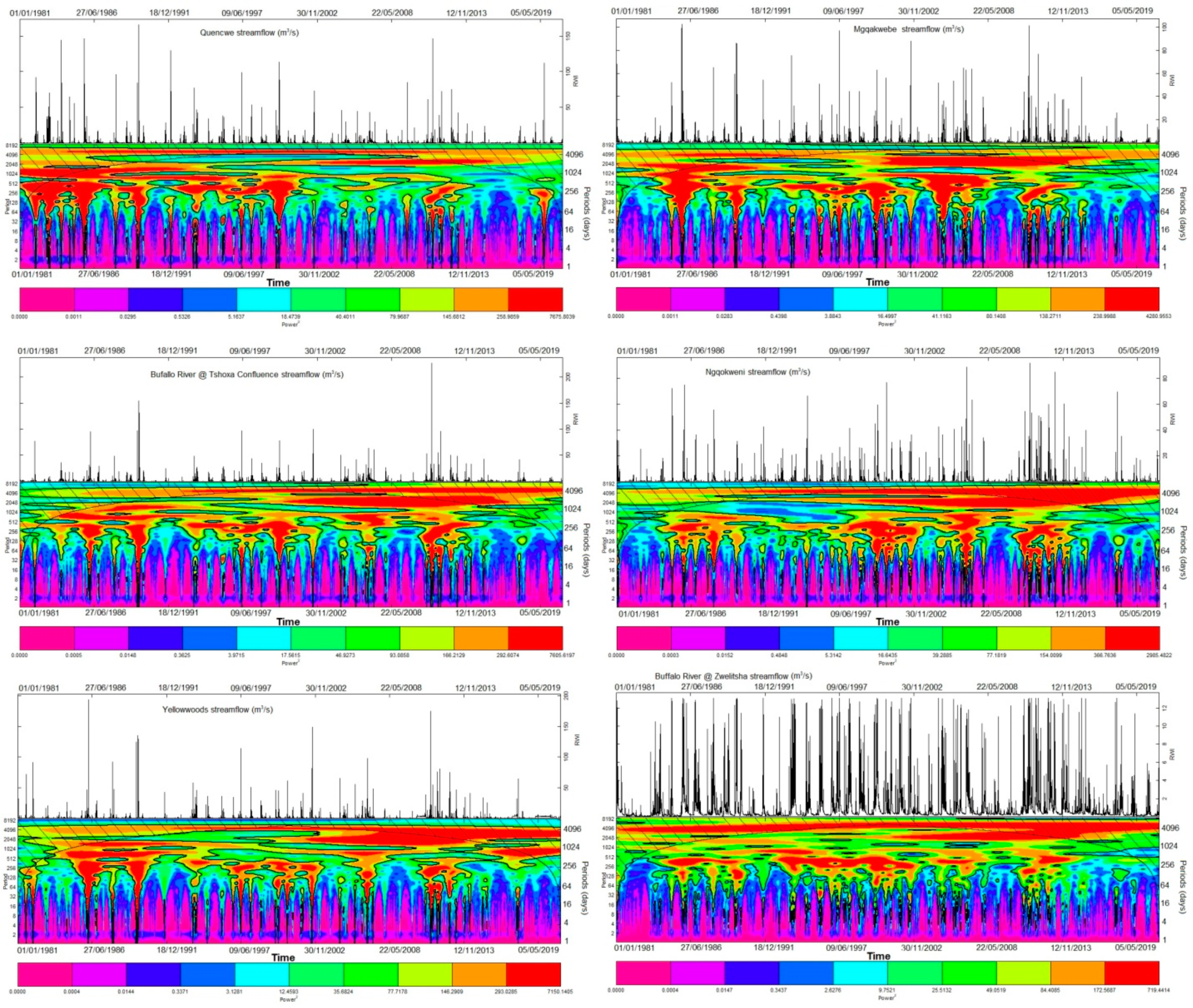
3.1. Continuous Wavelet Transform

The continuous wavelet transform (CWT) of the daily streamflow series (1981–2020) of stations in the Buffalo watershed was computed for information about the local wavelet spectral signal (Figure 2). The results show that the more substantial variability lies within the 128 and 4096-day scales. In most cases, substantial variability was exhibited at the periodic scale above 4096 days to 8192 days; however, these lie within the solid bell-shaped curved padding demarcating the possible erroneous zone affected by the edge effect. The most sporadic high-power signal, suggesting correlated wet days, in Quencwe, TB, Ngqokweni, and ZB streamflow were exhibited at scale 2048 days, while Mgqakwebe and Yellowwoods’ highest power lie on scale 4096 and 768 days. The most prominent region clustering, indicating the wetness period (less randomness) and streamflow persistence occurred slightly above 256 days, approximately a year.

The least inter-annual persistence, possibly due to dry spells, is exhibited at the upstream (Quencwe), indicating a sharp slump in high flow recurrence. The alteration gaps between any twain extreme signal are ranked in the order of reducing time-length: Quencwe > TB > Yellowwoods > Ngqokweni > Mgqakwebe > ZB. In the order of high-flow recurrence at a threshold of 80 m³/day from the first to the last, the Buffalo streamflow frequency can be ranked: Quencwe (15) > Yellowwoods (10) > Mgqakwebe (9) > TB (8) >Ngqokweni (5) > ZB (0). Buffalo streamflow intensity is exhibited in the following order from the most to the least: Quencwe (7676) > TB (7606) > Yellowwoods (7150) > Mgqakwebe (4281) > Ngqokweni (2985) > ZB (719). Ngqokweni streamflow showed a unique streamflow behavior that was quite gentle in the first half and sporadic in the second half of the time-scale. Both TB and Yellowwoods streamflow showed inter-annual persistence perceived to be intermittent in quinquennium. In contrast, the most significant persistence is shown by Mgqakwebe and downstream (ZB station).

3.2. Wavelet Coherence Analysis

The co-movement of streamflow and rainfall within the time-frequency domain is presented using the wavelet coherence scalograms (Figure 3). In this study, the co-movement exhibited at each station and the different multiscalar levels explain the dominant phase relationship. The assessment shows that streamflow and rainfall co-movement vary in time and space within the watershed across the scale of one month to 384 months (480 months). The hydro-climatic duo is significantly correlated across the short-, mid-, and long-term scales at the 0.05 significance level. The order of streamflow–rainfall scalar variability (1–160 months) across the station, that is, the total correlation of streamflow to rainfall, is exhibited as TB > Ngqokweni > Yellowwoods > Mgqakwebe > ZB > Quencwe.

Focusing on the low power level (1–4-month), only ZB (anti-phase), Ngqqokweni (in-phase), and Quencwe (lead-phase) streamflow–rainfall exhibit a significantly vital co-movement, with light co-movement depicted by TB (anti-phase), Mgqakwebe (lag-phase), and Yellowwoods (lag-phase). At the mid-power level (12–48 months), all the stations show a significantly strong correlation between streamflow–rainfall. Streamflow–rainfall co-movement levels are, accordingly: Quencwe (in-phase), Mgqakwebe (in-phase), TB (lead-lag phase), Ngqokweni (lead-phase), Yellowwoods (lag-phase), and ZB (lag-phase). At the high power level (120–480 months), some tangible information can be drawn from Buffalo’s main channel. TB depicts lag-phase inception, ZB suggests an overall in-phase, while Quencwe suggests the eventual in-phase relationship at the end of the time series.

3.3. Innovative Trend Analysis

The innovative trend analysis (ITA) of streamflow and hydro-climatic factors of the Buffalo catchment is presented as a scattered plot, divided across the regions of low (T < 33%), medium (33% ≤ T ≤ 67%), and high (T > 67%) attributes (Figure 4A–F;

Table 2. Statistical summary of ITA, lumped and summed MK statistics. The subscripts Sf, Rf, and Tp denote the computation for streamflow, rainfall, and temperature series. The bold figures and dates are the significant deductions and significant change-points while the negative and the positive results of T and Ԏ imply the decreasing and increasing trends of ITA and Mann–Kendall tests.

Data Series	ITA			Mann–Kendall			Pettitt Test
	TSf	TRf	TTp	ԎSf	ԎRf	ԎTp	KSf	KRf	KTp
Quencwe	−0.014	−0.081	0.001	−0.055	−0.070	0.023	January 2015	April 2013	October 2009
Mgqakwebe	−0.003	−0.084	0.001	0.034	−0.254	0.027	October 1996	January 2004	November 2002
Tshoxa Buff.	−0.192	−0.016	0.001	−0.103	−0.031	0.023	July 1987	June 2017	October 2009
Ngqokweni	0.002	−0.029	0.000	0.060	−0.028	0.020	November 1996	June 1997	August 2009
Yellowwoods	0.014	−0.071	0.001	0.213	−0.111	0.050	October 1996	July 2013	September 2013
Buffalo	−0.019	−0.131	0.001	0.050	−0.220	0.032	October 1996	July 2004	August 2009

). The ITA results showed that streamflow and rainfall across all the stations exhibit significant monotonic trends compared to temperature trends. The temperature trends tend to fluctuate from no trends to insignificant increasing trends across the medium to the high intensities temperature. Expectedly, this corresponds to the significantly decreasing trends exhibited by rainfall across all the stations. ITA shows that Buffalo watershed streamflow varies from a slight but tangible increasing low-flow (T = 0.002) trend to a strongly decreasing high-flow in the following order; Yellowwoods > Ngqokweni > Mgqakwebe > Quencwe > ZB > TB (Table 2). Only Yellowwoods streamflow showed a substantial increase in its low-flow and medium-flow trends, while Ngqokweni and Mgqakwebe streamflow showed an intangible increasing trend at the low-flow (Figure 4B,D,E). ZB station exhibits neutral to slightly decreasing streamflow trends while Quencwe and TB stations are characterized by a substantial decrease in trends across the entire flow attributes.

In comparison to rainfall trends, TB and Quencwe flow exhibit the most substantial sensitivity to the declining rainfall trends, with the streamflow deviating throughout the entire flow attributes (Figure 4A,C,F). Based on the flow attributes exhibited in the ITA plots, the three tributaries (Mgqakwebe, Ngqokweni, and Yellowwoods) and ZB showed remarkable insensitivity to rainfall trends. However, only ZB streamflow is elastic considering the concentration of medium flow. This finding conforms to the periodic variability of streamflow–rainfall co-movement shown on the WC plots.

In general, streamflow showed no virtual correlation with temperature, while the significant trend increase depicted by ITA rainfall can be associated with the increasing ITA temperature, though insignificant (Table 2; Figure 4).

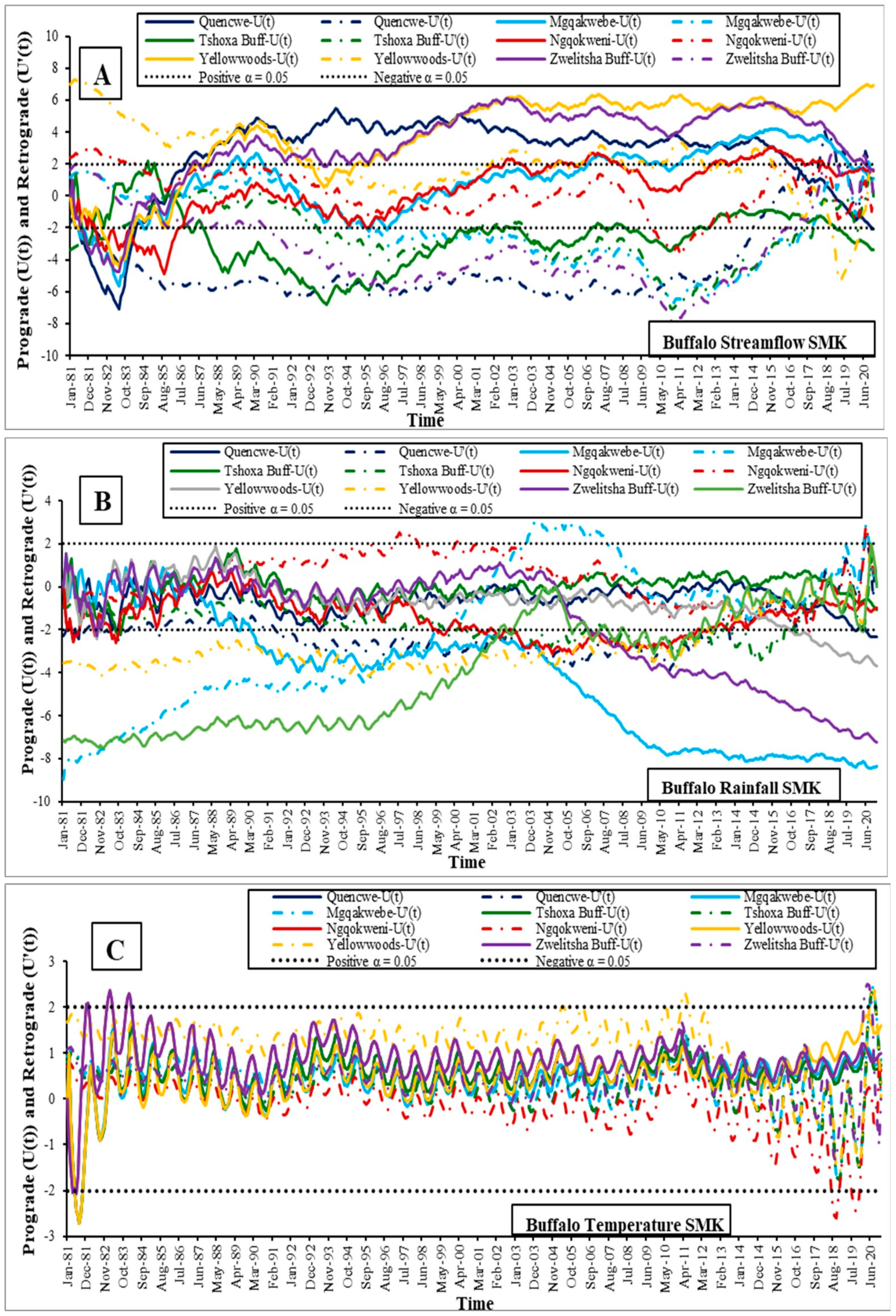
3.4. Mann-Kendall Trend Test and Sequential Mann-Kendall Analysis

The MK test and sequential MK (SMK) plots were performed with no whitening to ensure trend originality due to outliers at the test confidence levels of 5%. The MK trend test showed relative similarity in trend pattern to ITA. The rainfall trend depicts a substantial decrease across the stations compared to the temperature trend, exhibiting an insignificant increase (Figure 5B,C). Comparatively, the SMK provides a better visualization of variability across the time series compared to ITA, especially in the case of temperature trends within the insignificant region (Table 2; Figure 5A–C).

A critical assessment of the sequential MK analysis of the streamflow, rainfall, and temperature series of Buffalo stations depict four major trend turning points, principally in 1982–1983, 1992–1994, 2010–2011, and 2015–2020. The possible abrupt increase in the temperature occurred twice; in the winter months of 1982–1983 (1983, at high altitude and 1982 at the lower altitudes, Ngqokweni, and Buffalo meteorological stations) and in 2011 (across the stations). The abrupt slump in rainfall trends occurred once and varied across the stations with Mgqakwebe, ZB, Yellowwoods, Quencwe, and the remaining two stations occurring in November 1997, March 2007, April 2015, March 2017, and June 2018. The abrupt increase in streamflow trend occurred through 1992–1994 for the stations at the tributaries and Buffalo, while Quencwe and TB flow registered the abrupt decline in streamflow trend on 17 September and March 2018. The findings of the MK assessments correspond to the implication of the relative displacement of the streamflow–rainfall ITA slope.

3.5. Pettittt Change Point

The Pettitt test enabled the corroboration of the Mann–Kendall test by validating the insignificant change within the temperature series, even though the assessment indicated that the abrupt increase in the temperature was triggered in 1990. In the same vein, the assessment presents the specificity of the significant declining rainfall trends in 2004 and 2013 as identified by the MK and SMK plots. It also corroborates the significance of the streamflow change points across the station to the significant deductions shown by ITA. Compared to the SMK plot, 1995 and 1996 are the Pettitt periods of abrupt increase in streamflow, while 1987 and 2015 were the slump periods in the streamflow of the TB and Quencwe stations. The difference in the change points of SMK and Pettitt is because the Pettitt test is based on the breaking point of the maximum slope of the progressive series, while SMK depends on the interception point of the progressive and retrograde series.

4. Discussion

4.1. Characterization of Buffalo Streamflow Variability

The quantification of the streamflow process within a quasi-local scale has been achieved with the Continuous Wavelet Transform (CWT), projecting the inter-annual variability of daily streamflow across each sub-catchment. The result suggests that the dissimilarity remarks Buffalo streamflow in frequency, intensity, and length (periodicity) from upstream (Quencwe) to downstream (ZB). At the same time, the sub-catchments (Mgqakwebe, Ngqokweni, and Yellowwood) hydrological processes are self-contained [54,57,58]. The Innovative Trend Analysis reveals that the decline in high streamflow is due to the decrease in high (severe) and low (fractional) rainfall. This culminates into a recharge–storage–discharge system that favors the connected tributaries and increases in low streamflow, thus signaling the substantial groundwater–surface water discharge as a Buffalo River regressor during the dry spell.

Hence, the study shares a similar view on the possible controlling factors, which comprise the physiographic, hydrographic, and local climatic factors [4,28,31,69,82]. An elaborate discussion on the spatial variability of rainfall in a topographically complex environment under a monsoon climate system has been documented in the literature [7,21,82,83]. Moreover, Owolabi et al. [5] and Nolte et al. [3] extensively discussed the Buffalo catchment’s hydrographic properties and highlighted the tributary’s differential groundwater connection in enhancing the low-flow sessions and Buffalo’s perennial status. Owolabi et al. [6] noted a significant increase in winter (May–June–July) rainfall and streamflow trends and an insignificant decrease in the remaining part of the hydrologic regime. This possibly contributes to the streamflow increasing trends considering the unfavorable hydro-climatic distribution.

Flow attributes are either influenced by the hillslope or dam regulation by a comparative analysis of the abrupt change in streamflow intensity and streamflow–rainfall in-phase at Quencwe (Figure 3, Figure 4 and Figure 5A). Moreover, the groundwater recharge mechanism possibly impacted the rain–runoff high-flow imbalance, especially upstream, where the maximum rainfall and streamflow registered a percentage ratio of 94:30. More than half of the rainfall at a certain threshold is possibly recharged, compared to the Yellowwood station, where the percentage ratio of extreme rain-runoff is less than 1. This explains the streamflow lag on rainfall (Yellowwoods WC), possibly due to the drainage network and sub-basin morphogenetic development impacting extreme flow delivery in the Yellowwoods channel. Compared to other models, the integrated model here provides better visualization of hydrologic extremes hotspots.

The abrupt change in the runoff intensity due to the dam infrastructure and climatic variability possibly impact the midstream performance, characterized by a massive decline in supply relative to rainfall trends (Figure 3 and Figure 4). The seasonality of flow from the supply end possibly induces the dependency of Buffalo streamflow on rain, as shown by its short-term (1–4-month) and mid-term (8–64-month) sensitivity to rain, as well as the long-term persistence (Figure 3).

4.2. Buffalo Streamflow Response to Climate Change

The Buffalo River visibly exhibits high inter-annual variability, depicting periodic amplitude that divides approximately across decadal inter-annual nodes; 1989, 1999, 2010, and 2018, as projected by the CWT and SMK plots (Figure 2 and Figure 5). Jury [4] reported the impact of ENSO (El Niño–Southern Oscillation—the teleconnections between ocean–atmosphere coupling) and the 10-year inter-annual variability of South African rainfall. Varying intensity across all the stations exhibits other extreme events in 1985 and 2005. The correspondence of the extreme streamflow event (7676 cd) at the upstream with persistent recurrence of high-flow threshold (15 × 100 mm/day) and a long wet spell is typical of El Nino at the upstream and conversely at the downstream, depicting La Nina (Figure 2) [65].

The repression provided by the increasing temperature trend, decreasing rainfall distribution, and the accentuated response of streamflow dynamic also infers the imprint of climate change in Buffalo (Figure 4 and Figure 5; Table 2) [6,31]. The Pettitt test noted this in the spring of 1990 for temperature and highly variable rainfall (Table 2). The consistency of temperature and inconsistency of rainfall change points as a function of local and regional differences in response to climate change has been well articulated [15,84,85]. The periods of critical temperature increase (1982–1983, 1990, and 2011) and significant rainfall decline (1992–1996 and 2014–2020) exhibited by the SMK plots (Figure 4) conform to previous studies [7,14,21].

The SMK plots report a multi-year meteorological drought and result in a significant river diminution within those periods of extreme change in rainfall pattern. The perception is consistent with Mahlalela et al.’s [7] findings at the eastern and western flanks of the transition zone, computed using Climate Hazards Group InfraRed Precipitation with Station (CHIRPS) data. Mahlalela et al. [7] confirmed the impact of climate change by comparing dry and wet springs to the cyclone and anticyclone anomaly.

This study identifies the existence of resilience to the significant impact of climate change as a yardstick for selecting viable river channels (Figure 4 and Figure 5; Table 2). As a result, this study identifies the tributaries as the primary driver of the Buffalo River persistence, considering the significant flow increase exhibited. In conformity with this, the Pettitt test projected the uniform period of October 1996, indicating the period of the significant streamflow increase for the three stations as well as ZB.

4.3. Evaluation of the Integrated Framework Robustness

The integrated framework achieved profound hydro-statistical analysis, depicting the extreme events embedded in hydrological time series. Notably, the CWT enhances the visualization of the interannual variability of streamflow and its properties (frequency, length, and intensity) across different time scales. This was validated by SMK, which also buttresses MK deduction and corroborates ITA based on the periodic trends across time series. The contradictory values of ITA and SMK can be linked with the exertion of ITA on long-term flow duration differences. At the same time, MK employs the mean change across an estimated prograde and retrograde series. Essentially, ITA is weak for detecting instantaneous trends; however, it provides crucial information about the varying attributes of the flow sections. Moreover, the wavelet coherence appropriated the high degree of variability across the stations, capturing the persistence of streamflow across all levels in ZB stations. The Buffalo River across the second half of the time series while the antiphase correlation suggests the streamflow regress against the declining rainfall trends. The overall assessment shows that wavelet analysis needs to be corroborated to substantiate the extremities it provides, while SMK tends to be more versatile among all the methods used.

In general, the investigation suggests the predisposition of the watershed to extreme climatic changes with calls for the optimized exploitation of the upstream dam in the study area, although the average flow within the dam vicinity (TB) suggests its viability. The report on the Ngqokweni River’s elasticity shows that good environmental management practices were adhered to, despite its vulnerability (Table 1) [5]. The famishing nature of the Quencwe River is possibly due to the impact of the hillslope on its sustenance compared to the relatively plain Ngqokweni River. The Yellowwoods River also showed a high degree of conservation considering its trend increase during drought. In response to climate change, its inelastic flow might be due to its exploitation, which requires effective management against river diminution and drought risk.

5. Conclusions

The Buffalo catchment’s climatic significance and topographic complexity are essential factors in its streamflow dynamics. Considering this, the study area is an important site for demonstrating the numerical assessment and characterization of streamflow dynamics. In doing so, the reductionist approach at the headwater has proven reliable for simplifying streamflow processes. Moreover, the integrated framework provided tangible evidence of the extant impact of climate change. In addition, the following essential ramifications were drawn from the study:

• The robustness of continuous wavelet transform for analyzing tripartite streamflow property was distinctly portrayed;
• The assessment provides a simplified approach for investigating the hotspot of hydrologic extremes;
• The scale of investigation possibly influences the complexity of a hydrological process;
• The study provided substantial evidence of streamflow–ENSO teleconnection and projected the diminution of Buffalo streamflow;
• The Buffalo River is characterized as a rain-sensitive perennial channel, mainly replenished by its seasoned tributaries;
• Innovative trend analysis is quite limited in a numerical capacity as it could not provide tangible information or inference on change points.

The integrated framework employed here provides excellent insight into the performance of the catchment. Future studies may assess the ENSO relationship with the transition environment’s standard drought index considering the terrain’s sensitivity to climate change. The approach engaged here is reliable for adoption in hydro-meteorological assessment in any environment.

References

1. Brettenny, W.; Sharp, G. Efficiency evaluation of urban and rural municipal water service authorities in South Africa: A data envelopment analysis approach. Water SA 2016, 42, 11–19. [Google Scholar] [CrossRef]
2. Fanteso, B.; Yessoufou, K. Diversity and determinants of traditional water conservation technologies in the Eastern Cape Province, South Africa. Environ. Monit. Assess. 2022, 194, 1–14. [Google Scholar] [CrossRef] [PubMed]
3. Nolte, A.; Eley, M.; Schöniger, M.; Gwapedza, D.; Tanner, J.; Mantel, S.K.; Scheihing, K. Hydrological modelling for assessing spatio-temporal groundwater recharge variations in the water-stressed Amathole Water Supply System, Eastern Cape, South Africa: Spatially distributed groundwater recharge from hydrological model. Hydrol. Process. 2021, 35, 14264. [Google Scholar] [CrossRef]
4. Jury, M.R. Factors contributing to a decadal oscillation in South African rainfall. Theor. Appl. Climatol. 2014, 120, 227–237. [Google Scholar] [CrossRef]
5. Owolabi, S.T.; Madi, K.; Kalumba, A.M.; Baiyegunhi, C. A geomagnetic analysis for lineament detection and lithologic characterization impacting groundwater prospecting; a case study of Buffalo catchment, Eastern Cape, South Africa. Groundw. Sustain. Dev. 2021, 12, 100531. [Google Scholar] [CrossRef]
6. Owolabi, S.T.; Madi, K.; Kalumba, A.M. Comparative evaluation of Spatio-temporal attributes of precipitation and streamflow in Buffalo and Tyume Catchments, Eastern Cape, South Africa. Environ. Dev. Sustain. 2021, 23, 4236–4251. [Google Scholar] [CrossRef]
7. Mahlalela, P.T.; Blamey, R.C.; Hart, N.C.G.; Reason, C.J.C. Drought in the Eastern Cape region of South Africa and trends in rainfall characteristics. Clim. Dyn. 2020, 55, 2743–2759. [Google Scholar] [CrossRef]
8. Dube, R.A.; Maphosa, B.; Fayemiwo, O.M. Adaptive Climate Change Technologies and Approaches for Local Governments: Water Sector Response; WRC Report No. TT 663/16; Water Research Commission: Pretoria, South Africa, 2016. [Google Scholar]
9. Wannous, C.; Velasquez, G. United nations office for disaster risk reduction (UNISDR)—UNISDR’s contribution to science and technology for disaster risk reduction and the role of the international consortium on landslides (icl). In Workshop on World Landslide Forum (109–115); Springer: Cham, Switzerland, 2017. [Google Scholar]
10. UNISDR (United Nations International Strategy for Disaster Reduction). Impacts of Disasters since the 1992 Rio de Janeiro Earth Summit; UNISDR: Geneva, Switzerland, 2012. [Google Scholar]
11. Güneralp, B.; Güneralp, İ.; Liu, Y. Changing global patterns of urban exposure to flood and drought hazards. Glob. Environ. Chang. 2015, 31, 217–225. [Google Scholar] [CrossRef]
12. Chou, J.; Xian, T.; Dong, W.; Xu, Y. Regional temporal and spatial trends in drought and flood disasters in China and assessment of economic losses in recent years. Sustainability 2018, 11, 55. [Google Scholar] [CrossRef]
13. Rupa, R.C.; Mujumdar, P.P. Hydrologic impacts of climate change: Quantification of uncertainties. Proc. Indian Natl. Sci. Acad. 2019, 85, 77–94. [Google Scholar]
14. Pomposi, C.; Funk, C.; Shukla, S.; Harrison, L.; Magadzire, T. Distinguishing southern Africa precipitation response by the strength of El Niño events and implications for decision-making. Environ. Res. Lett. 2018, 13, 074015. [Google Scholar] [CrossRef]
15. Dong, Y.; Zhai, J.; Zhao, Y.; Wang, Q.; Jiang, S.; Chang, H.; Ding, Z. Teleconnection patterns of precipitation in the Three-River Headwaters region, China. Environ. Res. Lett. 2020, 15, 104050. [Google Scholar] [CrossRef]
16. Blamey, R.C.; Kolusu, S.R.; Mahlalela, P.; Todd, M.C.; Reason, C.J.C. The role of regional circulation features in regulating El Niño climate impacts over southern Africa: A comparison of the 2015/2016 drought with previous events. Int. J. Climatol. 2018, 38, 4276–4295. [Google Scholar] [CrossRef]
17. Worako, A.W.; Haile, A.T.; Taye, M.T. Streamflow variability and its linkage to ENSO events in the Ethiopian Rift Valley Lakes Basin. J. Hydrol. Reg. Stud. 2021, 35, 100817. [Google Scholar] [CrossRef]
18. Lee, D.; Ward, P.J.; Block, P. Identification of symmetric and asymmetric responses in seasonal streamflow globally to ENSO phase. Environ. Res. Lett. 2018, 13, 044031. [Google Scholar] [CrossRef]
19. Azharuddin, M.; Verma, S.; Verma, M.K.; Prasad, A.D. A Synoptic-Scale Assessment of Flood Events and ENSO—Streamflow Variability in Sheonath River Basin, India. In Advanced Modelling and Innovations in Water Resources Engineering; Springer: Singapore, 2022; pp. 93–104. [Google Scholar]
20. Lakhraj-Govender, R.; Grab, S.W. Assessing the impact of El Niño–Southern Oscillation on South African temperatures during austral summer. Int. J. Climatol. 2019, 39, 143–156. [Google Scholar] [CrossRef]
21. Blamey, R.C.; Ramos, A.M.; Trigo, R.M.; Tomé, R.; Reason, C.J.C. The influence of atmospheric rivers over the South Atlantic on winter rainfall in South Africa. J. Hydrometeorol. 2018, 19, 127–142. [Google Scholar] [CrossRef]
22. Adnan, R.M.; Zounemat-Kermani, M.; Kuriqi, A.; Kisi, O. Machine learning method in prediction streamflow considering periodicity component. In Intelligent Data Analytics for Decision-Support Systems in Hazard Mitigation; Springer: Singapore, 2021; pp. 383–403. [Google Scholar]
23. Pathak, P.; Kalra, A.; Ahmad, S.; Bernardez, M. Wavelet-aided analysis to estimate seasonal variability and dominant periodicities in temperature, precipitation, and streamflow in the Midwestern United States. Water Resour. Manag. 2016, 30, 4649–4665. [Google Scholar] [CrossRef]
24. Hwang, J.; Kumar, H.; Ruhi, A.; Sankarasubramanian, A.; Devineni, N. Quantifying Dam-Induced Fluctuations in Streamflow Frequencies Across the Colorado River Basin. Water Resour. Res. 2021, 57, e2021WR029753. [Google Scholar] [CrossRef]
25. Faiz, M.A.; Liu, D.; Fu, Q.; Li, M.; Baig, F.; Tahir, A.A.; Khan, M.I.; Li, T.; Cui, S. Performance evaluation of hydrological models using an ensemble of General Circulation Models in northeastern China. J. Hydrol. 2018, 565, 599–613. [Google Scholar] [CrossRef]
26. Kellner, E.; Hubbart, J.A. A method for advancing understanding of streamflow and eomorphological characteristics in mixed-land-use watersheds. Sci. Total Environ. 2019, 657, 634–643. [Google Scholar] [CrossRef] [PubMed]
27. Poff, N.L.; Allan, J.D.; Bain, M.B.; Karr, J.R.; Prestegaard, K.L.; Richter, B.D.; Sparks, R.E.; Stromberg, J.C. The natural flow regime: A paradigm for river conservation and restoration. BioScience 1997, 47, 769–784. [Google Scholar] [CrossRef]
28. Watson, A.; Miller, J.; Fink, M.; Kralisch, S.; Fleischer, M.; De Clercq, W. Distributive rainfall–runoff modelling to understand runoff-to-baseflow proportioning and its impact on the determination of reserve requirements of the Verlorenvlei estuarine lake, west coast, South Africa. Hydrol. Earth Syst. Sci. 2019, 23, 2679–2697. [Google Scholar] [CrossRef]
29. Asfaw, D.; Workineh, G. Quantitative analysis of morphometry on Ribb and Gumara watersheds: Implications for soil and water conservation. Int. Soil Water Conserv. Res. 2019, 7, 150–157. [Google Scholar] [CrossRef]
30. Skaggs, R.W.; Amatya, D.M.; Chescheir, G.M.; Blanton, C.D.; Gilliam, J.W. Effect of drainage and management practices on hydrology of pine plantation. In Hydrology and Management of Forested Wetlands, Proceedings of the International Conference, New Bern, NC, USA, 8–12 April 2006; American Society of Agricultural and Biological Engineers: St. Joseph, MI, USA, 2006; p. 3. [Google Scholar]
31. Owolabi, S.T.; Madi, K.; Kalumba, A.M.; Alemaw, B.F. Assessment of recession flow variability and the surficial lithology impact: A case study of Buffalo River catchment, Eastern Cape, South Africa. Environ. Earth Sci. 2020, 79, 1–19. [Google Scholar] [CrossRef]
32. Frey, S.K.; Miller, K.; Khader, O.; Taylor, A.; Morrison, D.; Xu, X.; Berg, S.J.; Hwang, H.T.; Sudicky, E.A.; Lapen, D.R. Evaluating landscape influences on hydrologic behavior with a fully-integrated groundwater–surface water model. J. Hydrol. 2021, 602, 126758. [Google Scholar] [CrossRef]
33. Frisbee, M.D.; Phillips, F.M.; Weissmann, G.S.; Brooks, P.D.; Wilson, J.L.; Campbell, A.R.; Liu, F. Unraveling the mysteries of the large watershed black box: Implications for the streamflow response to climate and landscape perturbations. Geophys. Res. Lett. 2012, 39. [Google Scholar] [CrossRef]
34. Boscarello, L.; Ravazzani, G.; Cislaghi, A.; Mancini, M. Regionalization of flow-duration curves through catchment classification with streamflow signatures and physiographic–climate indices. J. Hydrol. Eng. 2016, 21, 05015027. [Google Scholar] [CrossRef]
35. Knoben, W.J.; Woods, R.A.; Freer, J.E. A quantitative hydrological climate classification evaluated with independent streamflow data. Water Resour. Res. 2018, 54, 5088–5109. [Google Scholar] [CrossRef]
36. Sahraei, S.; Asadzadeh, M.; Unduche, F. Signature-based multi-modeling and multi-objective calibration of hydrologic models: Application in flood forecasting for Canadian Prairies. J. Hydrol. 2020, 588, 125095. [Google Scholar] [CrossRef]
37. Van Liew, M.W.; Arnold, J.G.; Garbrecht, J.D. Hydrologic simulation on agricultural watersheds: Choosing between two models. Trans. ASAE 2003, 46, 1539. [Google Scholar] [CrossRef]
38. Wagener, T.; Sivapalan, M.; Troch, P.; Woods, R. Catchment classification and hydrologic similarity. Geogr. Compass 2007, 1, 901–931. [Google Scholar] [CrossRef]
39. Castellarin, A.; Galeati, G.; Brandimarte, L.; Montanari, A.; Brath, A. Regional flow-duration curves: Reliability for ungauged basins. Adv. Water Resour. 2004, 27, 953–965. [Google Scholar] [CrossRef]
40. Botter, G.; Porporato, A.; Rodriguez-Iturbe, I.; Rinaldo, A. Basin-scale soil moisture dynamics and the probabilistic characterization of carrier hydrologic flows: Slow, leaching-prone components of the hydrologic response. Water Resour. Res. 2007, 43. [Google Scholar] [CrossRef]
41. Kamarudin, M.K.A.; Toriman, M.E.; Rosli, M.H.; Juahir, H.; Aziz, N.A.A.; Azid, A.; Zainuddin, S.F.M.; Sulaiman, W.N.A. Analysis of meander evolution studies on effect from land use and climate change at the upstream reach of the Pahang River, Malaysia. Mitig. Adapt. Strateg. Glob. Chang. 2015, 20, 1319–1334. [Google Scholar] [CrossRef]
42. Bergstrom, A.; Jencso, K.; McGlynn, B. Spatiotemporal processes that contribute to hydrologic exchange between hillslopes, valley bottoms, and streams. Water Resour. Res. 2016, 52, 4628–4645. [Google Scholar] [CrossRef]
43. Szilagyi, J.; Parlange, M.B. Baseflow separation based on analytical solutions of the Boussinesq equation. J. Hydrol. 1998, 204, 251–260. [Google Scholar] [CrossRef]
44. Bartlett, M.S.; Porporato, A. A class of exact solutions of the Boussinesq equation for horizontal and sloping aquifers. Water Resour. Res. 2018, 54, 767–778. [Google Scholar] [CrossRef]
45. Lebek, K.; Senf, C.; Frantz, D.; Monteiro, J.A.; Krueger, T. Interdependent effects of climate variability and forest cover change on streamflow dynamics: A case study in the Upper Umvoti River Basin, South Africa. Reg. Environ. Chang. 2019, 19, 1963–1971. [Google Scholar] [CrossRef]
46. Lupon, A.; Ledesma, J.L.; Bernal, S. Riparian evapotranspiration is essential to simulate streamflow dynamics and water budgets in a Mediterranean catchment. Hydrol. Earth Syst. Sci. 2018, 22, 4033–4045. [Google Scholar] [CrossRef]
47. Liu, W.; Wei, X.; Liu, S.; Liu, Y.; Fan, H.; Zhang, M.; Yin, J.; Zhan, M. How do climate and forest changes affect long-term streamflow dynamics? A case study in the upper reach of Poyang River basin. Ecohydrology 2015, 8, 46–57. [Google Scholar] [CrossRef]
48. Zhou, Y.; Zhang, Y.; Vaze, J.; Lane, P.; Xu, S. Impact of bushfire and climate variability on streamflow from forested catchments in southeast Australia. Hydrol. Sci. J. 2015, 60, 1340–1360. [Google Scholar] [CrossRef]
49. Mann, H.B. Nonparametric tests against trend. Econom. J. Econom. Soc. 1945, 13, 245–259. [Google Scholar] [CrossRef]
50. Yue, S.; Pilon, P.; Cavadias, G. Power of the Mann–Kendall and Spearman’s rho tests for detecting monotonic trends in hydrological series. J. Hydrol. 2002, 259, 254–271. [Google Scholar] [CrossRef]
51. Hamed, K.H.; Rao, A.R. A modified Mann-Kendall trend test for autocorrelated data. J. Hydrol. 1998, 204, 182–196. [Google Scholar] [CrossRef]
52. Sen, P.K. Estimates of the regression coefficient based on Kendall’s tau. J. Am. Stat. Assoc. 1968, 63, 1379–1389. [Google Scholar] [CrossRef]
53. Şen, Z. Innovative trend analysis methodology. J. Hydrol. Eng. 2012, 17, 1042–1046. [Google Scholar] [CrossRef]
54. Torrence, C.; Compo, G.P. A practical guide to wavelet analysis. Bull. Am. Meteorol. Soc. 1998, 79, 61–78. [Google Scholar] [CrossRef]
55. Coulibaly, P.; Burn, D.H. Wavelet analysis of variability in annual Canadian streamflows. Water Resour. Res. 2004, 40. [Google Scholar] [CrossRef]
56. Tamaddun, K.A.; Kalra, A.; Ahmad, S. Wavelet analyses of western US streamflow with ENSO and PDO. J. Water Clim. Chang. 2017, 8, 26–39. [Google Scholar] [CrossRef]
57. Domingues, M.O.; Mendes, O., Jr.; da Costa, A.M. On wavelet techniques in atmospheric sciences. Adv. Space Res. 2005, 35, 831–842. [Google Scholar] [CrossRef]
58. Hadi, S.J.; Tombul, M. Monthly streamflow forecasting using continuous wavelet and multi-gene genetic programming combination. J. Hydrol. 2018, 561, 674–687. [Google Scholar] [CrossRef]
59. Rösch, A.; Schmidbauer, H. WaveletComp 1.1: A Guided Tour through the R Package. 2016. Available online: http://www.hs-stat.com (accessed on 18 April 2022).
60. Ashraf, M.S.; Ahmad, I.; Khan, N.M.; Zhang, F.; Bilal, A.; Guo, J. Streamflow Variations in Monthly, Seasonal, Annual, and Extreme Values Using Mann-Kendall, Spearmen’s Rho and Innovative Trend Analysis. Water Resour. Manag. 2021, 35, 243–261. [Google Scholar] [CrossRef]
61. Sediqi, M.N.; Shiru, M.S.; Nashwan, M.S.; Ali, R.; Abubaker, S.; Wang, X.; Ahmed, K.; Shahid, S.; Asaduzzaman, M.; Manawi, S.M.A. A spatiotemporal pattern in the changes in availability and sustainability of water resources in Afghanistan. Sustainability 2019, 11, 5836. [Google Scholar] [CrossRef]
62. Kuriqi, A.; Ali, R.; Pham, Q.B.; Gambini, J.M.; Gupta, V.; Malik, A.; Linh, N.T.T.; Joshi, Y.; Anh, D.T.; Dong, X. Seasonality shift and streamflow flow variability trends in central India. Acta Geophys. 2020, 68, 1461–1475. [Google Scholar] [CrossRef]
63. Chauluka, F.; Singh, S.; Kumar, R. Rainfall and streamflow trends of Thuchila River, Southern Malawi. Mater. Today Proc. 2021, 34, 846–855. [Google Scholar] [CrossRef]
64. Kusangaya, S.; Toucher, M.L.W.; van Garderen, E.A. Evaluation of uncertainty in capturing the spatial variability and magnitudes of extreme hydrological events for the uMngeni catchment, South Africa. J. Hydrol. 2018, 557, 931–946. [Google Scholar] [CrossRef]
65. Philippon, N.; Rouault, M.; Richard, Y.; Favre, A. The influence of ENSO on winter rainfall in South Africa. Int. J. Climatol. 2012, 32, 2333–2347. [Google Scholar] [CrossRef]
66. Shamir, E.; Tapia-Villaseñor, E.M.; Cruz-Ayala, M.B.; Megdal, S.B. A review of climate change impacts on the USA-Mexico transboundary Santa Cruz River Basin. Water 2021, 13, 1390. [Google Scholar] [CrossRef]
67. Botai, C.M.; Botai, J.O.; Adeola, A.M.; De Wit, J.P.; Ncongwane, K.P.; Zwane, N.N. Drought risk analysis in the Eastern Cape Province of South Africa: The copula lens. Water 2020, 12, 1938. [Google Scholar] [CrossRef]
68. Grecksch, K. Adaptive capacity and water governance in the Keiskamma River catchment, Eastern Cape province, South Africa. Water SA 2015, 41, 359–368. [Google Scholar] [CrossRef]
69. Owolabi, S.T.; Madi, K.; Kalumba, A.M.; Orimoloye, I.R. A groundwater potential zone mapping approach for semi-arid environments using remote sensing (RS), geographic information system (GIS), and analytical hierarchical process (AHP) techniques: A case study of Buffalo catchment, Eastern Cape, South Africa. Arab. J. Geosci. 2020, 13, 1–17. [Google Scholar] [CrossRef]
70. Mishra, A.K.; Singh, V.P. Changes in extreme precipitation in Texas. J. Geophys. Res. Atmos. 2010, 115. [Google Scholar] [CrossRef]
71. Liu, H.; Yu, Y.; Zhao, W.; Guo, L.; Liu, J.; Yang, Q. Inferring subsurface preferential flow features from wavelet analysis of hydrological signals in the Shale Hills catchment. Water Resour. Res. 2020, 56, e2019WR026668. [Google Scholar] [CrossRef]
72. Lafreniere, M.; Sharp, M. Wavelet analysis of inter-annual variability in the runoff regimes of glacial and Nival stream catchments, Bow Lake, Alberta. Hydrol. Process. 2003, 17, 1093–1118. [Google Scholar] [CrossRef]
73. Roushangar, K.; Alizadeh, F.; Adamowski, J. Exploring the effects of climatic variables on monthly precipitation variation using a continuous wavelet-based multiscale entropy approach. Environ. Res. 2018, 165, 176–192. [Google Scholar] [CrossRef]
74. Tian, H.; Cazelles, B. WaveletCo: Wavelet Coherence Analysis; R Package Version 1.0. 2012. Available online: http://cran.r-project.org (accessed on 17 April 2022).
75. Wu, H.; Qian, H. Innovative trend analysis of annual and seasonal rainfall and extreme values in Shaanxi, China, since the 1950s. Int. J. Climatol. 2017, 37, 2582–2592. [Google Scholar] [CrossRef]
76. Gavrilov, M.B.; Tošić, I.; Marković, S.B.; Unkašević, M.; Petrović, P. Analysis of annual and seasonal temperature trends using the Mann-Kendall test in Vojvodina, Serbia. Időjárás 2016, 120, 183–198. [Google Scholar]
77. Hipel, K.W.; McLeod, A.I. Time Series Modelling of Water Resources and Environmental Systems; Electronic Reprint of Our Book Originally Published in 1994; Elsevier: Amsterdam, The Netherlands, 2005; Available online: http://www.stats.uwo.ca/faculty/aim/1994Book/ (accessed on 19 April 2022).
78. Sneyers, R. On the Statistical Analysis of Series of Observations (No. 551.501. 3 SNE.9); World Meteorological Organization: Geneva, Switzerland, 1990; pp. 1042–1046. [Google Scholar]
79. Pettitt, A.N. A non-parametric approach to the change-point problem. J. R. Stat. Soc. Ser. C (Appl. Stat.) 1979, 28, 126–135. [Google Scholar] [CrossRef]
80. Shen, D.; Bao, W.; Ni, P. A method for detecting abrupt change of sediment discharge in the Loess Plateau, China. Water 2018, 10, 1183. [Google Scholar] [CrossRef]
81. Verstraeten, G.; Poesen, J.; Demaree, G.; Salles, C. Long-term (105 years) variability in rain erosivity as derived from 10-min rainfall depth data for Ukkel (Brussels, Belgium): Implications for assessing soil erosion rates. J. Geophys. Res. 2006, 111, 22109. [Google Scholar] [CrossRef]
82. Shi, H.; Li, T.; Wei, J. Evaluation of the gridded CRU TS precipitation dataset with the point raingauge records over the Three-River Headwaters Region. J. Hydrol. 2017, 548, 322–332. [Google Scholar] [CrossRef]
83. Kukulies, J.; Chen, D.; Wang, M. Temporal and spatial variations of convection, clouds and precipitation over the Tibetan Plateau from recent satellite observations. Part II: Precipitation climatology derived from global precipitation measurement mission. Int. J. Climatol. 2020, 40, 4858–4875. [Google Scholar] [CrossRef]
84. Jiang, R.; Gan, T.Y.; Xie, J.; Wang, N. Spatiotemporal variability of Alberta’s seasonal precipitation, their teleconnection with large-scale climate anomalies and sea surface temperature. Int. J. Climatol. 2013, 34, 899–917. [Google Scholar] [CrossRef]
85. Barlow, M.; Gutowski, W.J.; Gyakum, J.R.; Katz, R.W.; Lim, Y.; Schumacher, R.S.; Wehner, M.F.; Agel, L.; Bosilovich, M.; Collow, A.; et al. North American extreme precipitation events and related large-scale meteorological patterns: A review of statistical methods, dynamics, modeling, and trends. Clim. Dyn. 2019, 53, 6835–6875. [Google Scholar] [CrossRef]
Figure 1. The map of the Buffalo River Basin showing the basin elevation and the six streamflow gauging stations: three stations on the main channel (Quencwe R., Tshoxa R. confluence, and the mouth before the Yellowwood R. confluence) and three stations on the tributaries (Mgqakwebe R., Ngqokweni R., and Yellowwoods R.).
Mathematics 10 03003 g001
Figure 2. The streamflow time series and the local power spectra for the period of 1 January 1980 to 30 December 2020 in the Buffalo River basin. The red region denotes the areas of high power values and a 5% significance level, while the cone of influence of the edge effects denoted by the diagonal webs are the cut-off regions of analytical errors.
Mathematics 10 03003 g002
Figure 3. Wavelet coherence analysis of daily rainfall and streamflow of Buffalo (1981–2020) and their wavelet spectrum. The power level ranges from zero intensity (Blue) to high intensity (Red) at a 95% confidence level. The cloudy/white transparent cover demarcates the border of the edge effect interpretation. The right (left) pointing black arrow denotes an in-phase (antiphase) correlation between the streamflow and rainfall, while the upward (downward) arrow denotes that streamflow leads (lags behind) rainfall by 90°.
Mathematics 10 03003 g003
Figure 4. The plot of the innovative trends analysis of the Buffalo catchment rainfall (blue), streamflow (yellow), and temperature (red) dataset (1981–2020) for: (A). Quencwe station, (B). Mgqakwebe, (C). Tshoxa Buffalo station, (D). Ngqokweni station, (E). Yellowwoods station, and (F). Zwelitsha Buffalo station. The central thick line denotes the zero trend line. The dotted diagonal lines on the two sides of the zero trend line denote the significant level (α = 0.05).
Mathematics 10 03003 g004
Figure 5. The plot of sequential Mann–Kendall trend analysis showing; (A). monthly streamflow, (B). rainfall, and (C). temperature series (1981–2020). The dotted horizontal lines on the positive (Pos) and negative (Neg) sides of the y-axis identify the significance level (α = 0.05). The straight and dotted plots indicate the prograde (U(t)) and retrograde (U′(t)) series.
Mathematics 10 03003 g005