
Gain-Scheduled Sliding-Mode-Type Iterative Learning Control Design for Mechanical Systems
by
 , , and
Qijia Yao
1 ,
,
Hadi Jahanshahi
2,
Stelios Bekiros
3,4,5,
Sanda Florentina Mihalache
6,* and
and
Naif D. Alotaibi
7 1
School of Aerospace Engineering, Beijing Institute of Technology, Beijing 100081, China
2
Department of Mechanical Engineering, University of Manitoba, Winnipeg, MB R3T 5V6, Canada
3
FEMA, University of Malta, MSD 2080 Msida, Malta
4
LSE Health, Department of Health Policy, London School of Economics and Political Science, London WC2 A2 AE, UK
5
IPAG Business School, 184 Boulevard Saint-Germain, 75006 Paris, France
6
Automatic Control, Computers & Electronics Department, Petroleum-Gas University of Ploiești, 100680 Ploiești, Romania
7
Department of Electrical and Computer Engineering, Faculty of Engineering, King Abdulaziz University, Jeddah 21589, Saudi Arabia
*
Author to whom correspondence should be addressed.
Mathematics 2022, 10(16), 3005; https://doi.org/10.3390/math10163005
Submission received: 17 July 2022
/
Revised: 14 August 2022
/
Accepted: 18 August 2022
/
Published: 20 August 2022
(This article belongs to the Special Issue Control Problem of Nonlinear Systems with Applications)
Abstract
:In this paper, a novel gain-scheduled sliding-mode-type (SM-type) iterative learning (IL) control approach is proposed for the high-precision trajectory tracking of mechanical systems subject to model uncertainties and disturbances. Based on the SM variable, the proposed controller is synthesized involving a feedback regulation item, a feedforward learning item, and a robust switching item. The feedback regulation item is adopted to regulate the position and velocity tracking errors, the feedforward learning item is applied to handle the model uncertainties and repetitive disturbance, and the robust switching item is introduced to compensate the nonrepetitive disturbance and linearization residual error. Moreover, the gain-scheduled mechanism is employed for both the feedback regulation item and feedforward learning item to enhance the convergence speed. Convergence analysis illustrates that the position and velocity tracking errors can eventually regulate to zero under the proposed controller. By combining the advantages of both SM control and IL control, the proposed controller has strong robustness against model uncertainties and disturbances. Lastly, simulations and comparisons are provided to evaluate the efficiency and excellent performance of the proposed control approach.
Keywords:
mechanical system; sliding-mode-type iterative learning control; trajectory tracking control; gain-scheduled mechanismMSC:
70E60; 70Q05; 93C15; 93C401. Introduction
Many advanced control methods have been introduced in [1,2,3,4,5,6,7,8,9,10,11,12,13,14,15,16,17,18]. Iterative learning (IL) control is a memory-based control approach for the control plants which execute repeated or periodic operations over a finite time domain. The IL control can gradually improve the control performance by learning from the experience of previous iterations. According to the utilization of different feedback regulators, the IL control can be mainly classified into the proportional-type (P-type) IL control, differential-type (D-type) IL control, proportional–differential-type (PD-type) IL control, and proportional–integral–differential-type (PID-type) IL control. A survey on IL control and its applications can be found in [19,20,21,22]. The IL control has the major advantage that it does not require an accurate system model or even does not need any prior system information, which brings a great convenience to the controller design. Since the pioneering work by Arimoto et al. [23] in 1984, the IL control has been broadly utilized for the control of a large range of mechanical systems, such as robotic manipulators [24,25,26,27,28,29,30,31,32,33], robotic fish [34,35], mobile robots [36,37], spacecraft [38,39,40], and permanent magnet spherical actuators [41].
Although the IL control has been extensively developed, there are still some research issues remaining not well addressed. Among these issues, the robustness and convergence speed of the controller are two major concerns. During the practical applications, the mechanical system is unavoidably affected by model uncertainties and disturbances. The robust IL control is a good solution to such problems, with strong robustness against model uncertainties and disturbances. A commonly used robust IL control method is integrating the IL control with some compensation tools, such as neural network [42,43,44,45], fuzzy logic system [46,47], and disturbance observer [48,49]. However, these approaches more or less increase the structural complexity of the controller. Moreover, the sliding-mode-type (SM-type) IL control is another effective robust IL control method. As a new type of IL control, the SM-type IL control combines the advantages of both SM control and IL control. Chen et al. [50] designed a robust IL controller for the output tracking of an SRV02 rotary plant by utilizing the second-order SM control technique. In [51], an SM-type IL control approach was developed for the wire tension control of an automatic motor winding machine. In [52], a constant-force control method was proposed for the robotic belt grinding by integrating adaptive SM control with IL control. Nguyen et al. [53] designed an SM-type IL control for the trajectory tracking of a quadrotor unmanned aerial vehicle subject to model uncertainties and external disturbances. Zhang et al. [54] proposed an adaptive SM-type IL control scheme for non-repetitive tasks of a upper-limb exoskeleton with output constraints. In [55], an intelligent model-free controller was constructed for a tray indexing system with unknown dynamics by combining IL control and super-twisting SM control. Wang et al. [56] presented a global SM-type IL control approach for the contouring motion tasks of an industrial biaxial gantry system. In [57], a neural network-based SM-type IL controller was implemented to a permanent-magnet synchronous motor with uncertainties and external disturbances.
It should be pointed out that the convergence speed is another critical performance index for the IL control. Nevertheless, the convergence speed is not sufficiently considered in the above SM-type IL control design. The constant iteration gains are employed in most of the aforementioned SM-type IL controllers, resulting in the relatively slow convergence speed. The adaptive IL control is an efficient approach to accelerate the convergence by designing the adaptive iteration gains. To accelerate the convergence, a fundamental idea of the adaptive IL control is adopting relatively small gains at the initial iterations and gradually enlarging the gains with the iteration number increasing. Some existing adaptive gain-scheduled strategies can be found in [29,30,31,32,36,39,41]. However, to the best of our knowledge, there are limited studies focused on IL control with the consideration of strong robustness and fast convergence speed simultaneously. Indeed, the robust IL control design with fast convergence speed is still a challenging problem currently, which deserves to be further addressed.
Inspired by the above discussions, we propose a novel gain-scheduled SM-type IL control approach for the high-precision trajectory tracking of mechanical systems subject to model uncertainties and disturbances. Both strong robustness and fast convergence speed are included in the proposed control design. Compared to most previous research, the main novelties and contributions of this work are presented as follows.
- The proposed controller is synthesized involving a feedback regulation item, a feedforward learning item, and a robust switching item. By combining the advantages of both SM control and IL control, the proposed controller has strong robustness against model uncertainties and disturbances.
- The gain-scheduled mechanism is employed for both the feedback regulation item and feedforward learning item. Benefiting from this design, the proposed controller can achieve relatively fast convergence speed.
- Convergence analysis is theoretically provided. The proposed controller can ensure the position and velocity tracking errors can eventually regulate to zero even in the presence of model uncertainties and disturbances.
2. Problem Description
Consider the trajectory tracking of a large range of mechanical systems whose dynamics can be described in Euler–Lagrangian form (1),
where and are the position and velocity of the mechanical system, is the inertia matrix, is the Coriolis and centrifugal matrix, is the gravitational vector, represents the control inputs, and represents the disturbances. When considering model uncertainties, the matrices , , and can be rewritten as , , and , where , , and are the nominal parts and , , and are the unknown parts. Moreover, the disturbances can be rewritten as , where and are the repetitive and nonrepetitive disturbances, respectively. Define the lumped model uncertainties as . Subsequently, system (1) can be rearranged as (2),
According to [58], system (2) has the following fundamental properties.
Property 1.
The matrixis positive definite and bounded.
Property 2.
The matrixis skew symmetric.
Let be the desired position to be tracked. Define as the position tracking errors, and then the velocity tracking errors can be expressed as . Employing the Taylor expansion, the linearized dynamic model of the mechanical system along the desired trajectory can be calculated as (3),
where , , , , , and is the linearization residual error. Thus, the linearized dynamic model of the mechanical system for the th iteration can be described as (4),
The aim of this research is developing a controller to ensure the desired position and velocity of the mechanical system can be eventually tracked under model uncertainties and disturbances, when , , and . Before proceeding, standard assumptions are made as follows.
Assumption 1.
The model uncertainties and disturbances,,,, andare bounded.
Assumption 2.
The initial conditions for each iteration are identical,and.
3. Controller Design
In this section, an innovative gain-scheduled SM-type IL controller is developed to solve the above trajectory tracking problem. First, the SM variable for the th iteration is introduced as (5),
where . Then, the gain-scheduled SM-type IL controller for the th iteration is synthesized as (6),
where is the feedback regulation item, is the feedforward learning item, and is the robust switching item. The expressions of , , and are presented as (7)–(9), respectively:
where , , , , and represents the signum function. The gain matrices and are exponentially scheduled through the mechanism designed as (10),
where , , and are the positive definite gain matrices for the initial iteration.
Remark 1.
The proposed controller (6) involves the feedback regulation item (7), the feedforward learning item (8), and the robust switching item (9). The feedback regulation item is adopted to regulate the position and velocity tracking errors, the feedforward learning item is applied to handle the model uncertainties and repetitive disturbance, and the robust switching item is introduced to compensate the nonrepetitive disturbance and linearization residual error.
Remark 2.
Moreover, the gain-scheduled mechanism (10) is employed and the gain matrices of both the feedback regulation item and feedforward learning item are exponentially scheduled from iteration to iteration. For the initial iteration, the position and velocity tracking errors are relatively large. At this moment, the gain matrices are set small to avoid the control toques out of the reasonable range. As the iteration number increases, the position and velocity tracking errors are degraded. At this moment, the gain matrices become large enough through the mechanism (10) to enhance the convergence speed of the proposed controller.
Remark 3.
To give the readers a better understanding of the whole control design procedure, the structure of the proposed gain-scheduled SM-type IL control approach is provided in Figure 1.
Remark 4.
A weakness of the proposed controller is that it is designed under the assumption of the identical initial conditions for each iteration. This assumption is commonly made in the previous research on IL control. Nevertheless, such an assumption is quite conservative for practical systems. Our future research will focus on removing this assumption, and the ideas in [59,60,61,62] may provide the guideline.
4. Convergence Analysis
In this section, the convergence of the proposed controller is analyzed through the main theorem as follows.
Theorem 1.
Consider the mechanical system (1) controlled by the SM-type IL controller (6) and the gain-scheduled mechanism (10). If the control gains are properly determined satisfying the conditions (11)–(14),
Proof.
The Lyapunov function for the th iteration is presented as (15),
where and . Define . Then, can be calculated as (16):
The linearized dynamic model of the mechanical system for the th iteration can be described as (17),
Combining (4) and (17), we can obtain (18),
where and . Employing (6), can be calculated as (19),
Combining (18) and (19), can be calculated as (20),
where . Rearranging (20), can be calculated as (21),
Substituting (21) into (16), we can obtain (22),
Since , Equation (23) can be obtained through the integration by parts,
Rearranging (23), can be calculated as (24),
Moreover, inequality (25) can easily be derived:
Substituting (24) and (25) into (23), we can obtain (26),
where . Since , Equation (27) can be obtained through the integration by parts,
Rearranging (27), can be calculated as (28),
Substituting (28) into (27), we can obtain (29),
where . From conditions (11)–(13), inequality (30) can be derived:
Moreover, from condition (14), inequality (31) can be derived:
Substituting (30) and (31) into (29), we can obtain (32),
This means that . Moreover, from the definition of , we have and is bounded. Thus, we can derive that when , . Combined with the definition of , we further have that when , and . This finishes the proof. □
5. Simulations and Comparisons
In this section, simulations and comparisons are provided to demonstrate the efficiency and advantages of the proposed controller. The simulation scenario is considered as the trajectory tracking control of a two-link robot manipulator, as shown in Figure 2, whose dynamics can be described as system (1) with the expressions of , , and , given as (33) [58],
where , , , , , , , , , , , , , , and . Moreover, the meanings of the physical and geometric parameters , , , , , , , and can be found in Figure 2.
In the simulations, the physical and geometric parameters of the robot manipulator are chosen as , , , , , , , and . The disturbances are given as . The desired trajectory of the robot manipulator is chosen as . Accordingly, the initial position and velocity of the robot manipulator are set as and , respectively. Moreover, the control gains of the proposed gain-scheduled SM-type IL controller are selected as , , , , and .
The simulation results for the proposed controller under the first five iterations are provided in Figure 3, Figure 4, Figure 5, Figure 6 and Figure 7. Figure 3 and Figure 4 show the time response of the position tracking and velocity tracking under the first five iterations. It is clearly seen that as the iteration number increases, the actual position and velocity of the robot manipulator can regulate to the desired values more accurately and rapidly. The time response of the control torques under the first five iterations is given in Figure 5. It is obvious that the control torques can always stay within the reasonable range during the whole trajectory tracking process. Figure 6 and Figure 7 present the maximum absolute errors (MAEs) of the position tracking and velocity tracking under the first five iterations. The MAEs greatly decrease for the first three iterations and then they tend to be steady. Under the fourth iteration, the MAEs of the position tracking are and , and the MAEs of the velocity tracking are and . It is noteworthy that such tracking accuracy is sufficient for the operations of industrial robots in the real world.
Besides the proposed controller, the finite-time PD-like controller based on the homogeneous method in [63] is also employed for comparisons, which is designed as (34),
where , , , , and represents . Note that large gains and can result in the relative fast convergence speed, but the control torques may become relatively large at the same time. In the simulations, the control gains of the compared finite-time PD-like controller are selected as , , , and through trial and error.
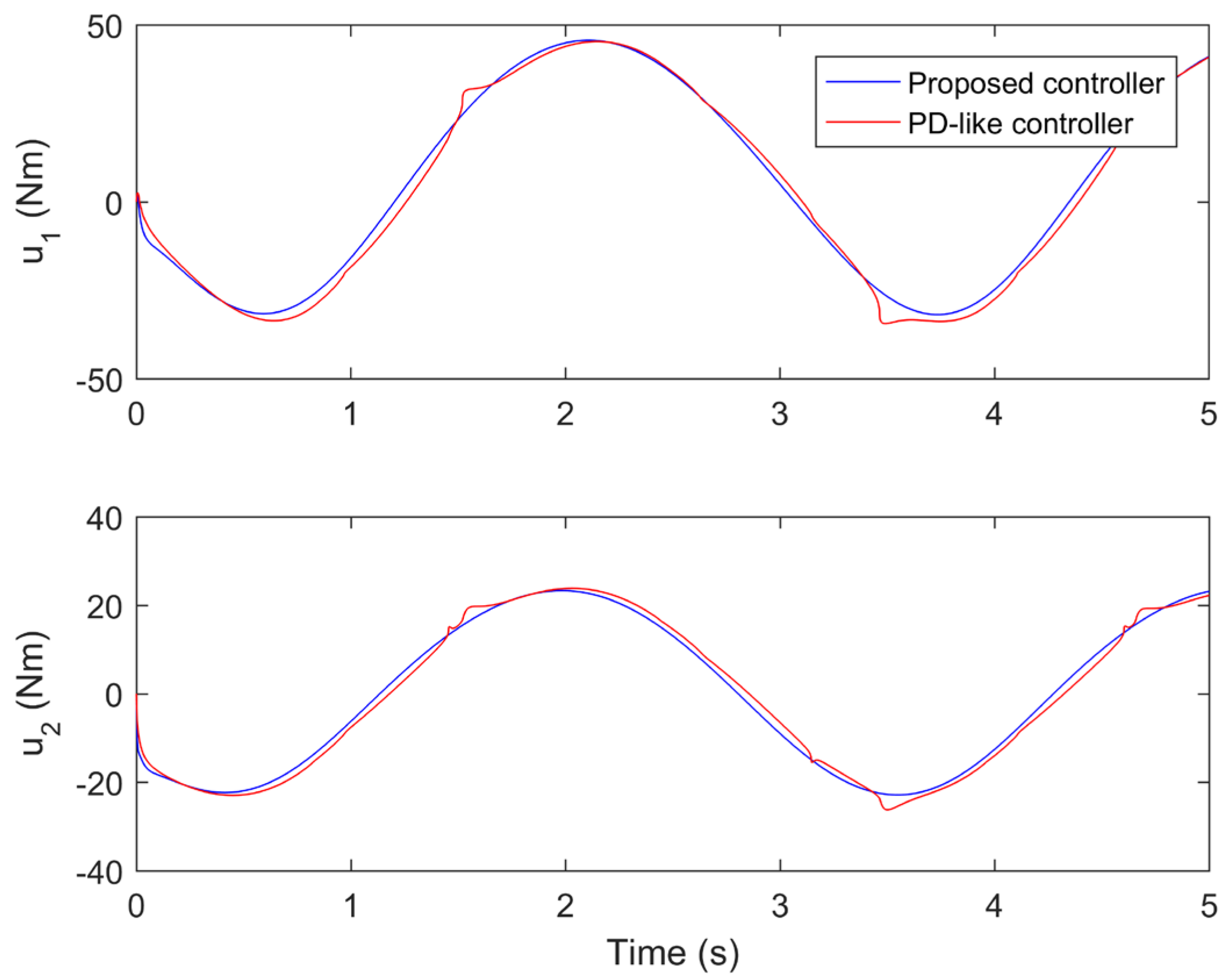
The performance comparisons between the proposed controller under the fourth iteration and the compared finite-time PD-like controller are provided in Figure 8, Figure 9, Figure 10, Figure 11 and Figure 12. Figure 8 and Figure 9 present the tine response of the position tracking and velocity tracking under both controllers. Figure 10 and Figure 11 give the tine response of the position and velocity tracking errors under both controllers. Moreover, the time responses of the control torques under both controllers are shown in Figure 12.
From Figure 10 and Figure 11, the steady-state position and velocity tracking errors under the compared finite-time PD-like controller are much larger than those under the proposed controller. The proposed controller can realize the high-performance trajectory tracking of robot manipulator even subject to model uncertainties and disturbances. However, the tracking performance of the compared finite-time PD-like controller is relatively poor under the same conditions. This means the proposed controller is strongly robust against model uncertainties and disturbances. The strong robustness of the proposed controller is mainly because it combines the advantages of both SM control and IL control. Moreover, it is not difficult to find that the settling time under the compared finite-time PD-like controller is also quite longer than that under the proposed controller. This means the proposed controller has relatively fast convergence speed. The fast convergence speed of the proposed controller is benefiting from the utilization of gain-scheduled mechanism. From the simulation results, it is concluded that the proposed controller can achieve better tracking performance than the compared finite-time PD-like controller in terms of higher steady-state accuracy and faster convergence speed.
6. Conclusions
We propose a novel gain-scheduled SM-type IL control approach for the high-precision trajectory tracking of mechanical systems subject to model uncertainties and disturbances. Specifically, the proposed controller involves a feedback regulation item to regulate the position and velocity tracking errors, a feedforward learning item to handle the model uncertainties and repetitive disturbance, and a robust switching item to compensate the nonrepetitive disturbance and linearization residual error. Moreover, the gain matrices of both the feedback regulation item and feedforward learning item are exponentially scheduled to enhance the convergence speed. The proposed controller can ensure the position and velocity tracking errors eventually regulate to zero through convergence analysis. Lastly, the efficiency and advantages of the proposed controller are verified by simulations and comparisons. It is expected that the proposed control approach can provide a beneficial reference for the high-precision control of industrial robots in the real world.
Author Contributions
Conceptualization, Q.Y., H.J., S.B., S.F.M. and N.D.A.; methodology, Q.Y., H.J., S.B., S.F.M. and N.D.A.; software, Q.Y., H.J., S.B., S.F.M. and N.D.A.; validation, Q.Y., H.J., S.B., S.F.M. and N.D.A.; writing—original draft preparation, Q.Y., H.J., S.B., S.F.M. and N.D.A.; writing—review and editing, Q.Y., H.J., S.B., S.F.M. and N.D.A.; supervision, Q.Y., H.J., S.B., S.F.M. and N.D.A. All authors have read and agreed to the published version of the manuscript.
Funding
The Deanship of Scientific Research (DSR) at King Abdulaziz University, Jeddah, Saudi Arabia has funded this project, under grant no. (FP-024-43).
Institutional Review Board Statement
Not applicable.
Informed Consent Statement
Not applicable.
Data Availability Statement
Not applicable.
Conflicts of Interest
The authors declare no conflict of interest.
References
- Wang, B.; Jahanshahi, H.; Volos, C.; Bekiros, S.; Khan, M.A.; Agarwal, P.; Aly, A.A. A new RBF neural network-based fault-tolerant active control for fractional time-delayed systems. Electronics 2021, 10, 1501. [Google Scholar] [CrossRef]
- Jahanshahi, H.; Yousefpour, A.; Wei, Z.; Alcaraz, R.; Bekiros, S. A financial hyperchaotic system with coexisting attractors: Dynamic investigation, entropy analysis, control and synchronization. Chaos Solitons Fractals 2019, 126, 66–77. [Google Scholar] [CrossRef]
- Wang, Y.-L.; Jahanshahi, H.; Bekiros, S.; Bezzina, F.; Chu, Y.-M.; Aly, A.A. Deep recurrent neural networks with finite-time terminal sliding mode control for a chaotic fractional-order financial system with market confidence. Chaos Solitons Fractals 2021, 146, 110881. [Google Scholar] [CrossRef]
- Kosari, A.; Jahanshahi, H.; Razavi, S.A. An optimal fuzzy PID control approach for docking maneuver of two spacecraft: Orientational motion. Eng. Sci. Technol. Int. J. 2017, 20, 293–309. [Google Scholar] [CrossRef] [Green Version]
- Li, J.-F.; Jahanshahi, H.; Kacar, S.; Chu, Y.-M.; Gómez-Aguilar, J.F.; Alotaibi, N.D.; Alharbi, K.H. On the variable-order fractional memristor oscillator: Data security applications and synchronization using a type-2 fuzzy disturbance observer-based robust control. Chaos Solitons Fractals 2021, 145, 110681. [Google Scholar] [CrossRef]
- Wang, B.; Jahanshahi, H.; Arıcıoğlu, B.; Boru, B.; Kacar, S.; Alotaibi, N.D. A variable-order fractional neural network: Dynamical properties, Data security application, and synchronization using a novel control algorithm with a finite-time estimator. J. Frankl. Inst. 2022. [Google Scholar] [CrossRef]
- Alsaade, F.W.; Jahanshahi, H.; Yao, Q.; Al-zahrani, M.S.; Alzahrani, A.S. A new neural network-based optimal mixed H2/H∞ control for a modified unmanned aerial vehicle subject to control input constraints. Adv. Space Res. 2022. [Google Scholar] [CrossRef]
- Zhou, S.-S.; Jahanshahi, H.; Din, Q.; Bekiros, S.; Alcaraz, R.; Alassafi, M.O.; Alsaadi, F.E.; Chu, Y.-M. Discrete-time macroeconomic system: Bifurcation analysis and synchronization using fuzzy-based activation feedback control. Chaos Solitons Fractals 2021, 142, 110378. [Google Scholar] [CrossRef]
- Xiong, P.-Y.; Jahanshahi, H.; Alcaraz, R.; Chu, Y.-M.; Gómez-Aguilar, J.F.; Alsaadi, F.E. Spectral entropy analysis and synchronization of a multi-stable fractional-order chaotic system using a novel neural network-based chattering-free sliding mode technique. Chaos Solitons Fractals 2021, 144, 110576. [Google Scholar] [CrossRef]
- Jahanshahi, H.; Yousefpour, A.; Soradi-Zeid, S.; Castillo, O. A review on design and implementation of type-2 fuzzy controllers. Math. Methods Appl. Sci. 2022. [Google Scholar] [CrossRef]
- Jahanshahi, H.; Zambrano-Serrano, E.; Bekiros, S.; Wei, Z.; Volos, C.; Castillo, O.; Aly, A.A. On the dynamical investigation and synchronization of variable-order fractional neural networks: The Hopfield-like neural network model. Eur. Phys. J. Spec. Top. 2022, 231, 1757–1769. [Google Scholar] [CrossRef]
- Jahanshahi, H.; Yousefpour, A.; Munoz-Pacheco, J.M.; Kacar, S.; Pham, V.-T.; Alsaadi, F.E. A new fractional-order hyperchaotic memristor oscillator: Dynamic analysis, robust adaptive synchronization, and its application to voice encryption. Appl. Math. Comput. 2020, 383, 125310. [Google Scholar] [CrossRef]
- Jahanshahi, H.; Yousefpour, A.; Munoz-Pacheco, J.M.; Moroz, I.; Wei, Z.; Castillo, O. A new multi-stable fractional-order four-dimensional system with self-excited and hidden chaotic attractors: Dynamic analysis and adaptive synchronization using a novel fuzzy adaptive sliding mode control method. Appl. Soft Comput. 2020, 87, 105943. [Google Scholar] [CrossRef]
- Jahanshahi, H.; Rajagopal, K.; Akgul, A.; Sari, N.N.; Namazi, H.; Jafari, S. Complete analysis and engineering applications of a megastable nonlinear oscillator. Int. J. Non-Linear Mech. 2018, 107, 126–136. [Google Scholar] [CrossRef]
- Bekiros, S.; Jahanshahi, H.; Bezzina, F.; Aly, A.A. A novel fuzzy mixed H2/H∞ optimal controller for hyperchaotic financial systems. Chaos Solitons Fractals 2021, 146, 110878. [Google Scholar] [CrossRef]
- Jahanshahi, H.; Shahriari-Kahkeshi, M.; Alcaraz, R.; Wang, X.; Singh, V.P.; Pham, V.-T. Entropy analysis and neural network-based adaptive control of a non-equilibrium four-dimensional chaotic system with hidden attractors. Entropy 2019, 21, 156. [Google Scholar] [CrossRef] [PubMed] [Green Version]
- Jahanshahi, H. Smooth control of HIV/AIDS infection using a robust adaptive scheme with decoupled sliding mode supervision. Eur. Phys. J. Spec. Top. 2018, 227, 707–718. [Google Scholar] [CrossRef]
- Jahanshahi, H.; Sajjadi, S.S.; Bekiros, S.; Aly, A.A. On the development of variable-order fractional hyperchaotic economic system with a nonlinear model predictive controller. Chaos Solitons Fractals 2021, 144, 110698. [Google Scholar] [CrossRef]
- Xu, J.-X. A survey on iterative learning control for nonlinear systems. Int. J. Control 2011, 84, 1275–1294. [Google Scholar] [CrossRef]
- Ahn, H.-S.; Chen, Y.; Moore, K.L. Iterative learning control: Brief survey and categorization. IEEE Trans. Syst. Man Cybern. Part C Appl. Rev. 2007, 37, 1099–1121. [Google Scholar] [CrossRef]
- Bristow, D.A.; Tharayil, M.; Alleyne, A.G. A survey of iterative learning control. IEEE Control Syst. Mag. 2006, 26, 96–114. [Google Scholar]
- Moore, K.L.; Dahleh, M.; Bhattacharyya, S.P. Iterative learning control: A survey and new results. J. Robot. Syst. 1992, 9, 563–594. [Google Scholar] [CrossRef]
- Arimoto, S.; Kawamura, S.; Miyazaki, F. Bettering operation of robots by learning. J. Robot. Syst. 1984, 1, 123–140. [Google Scholar] [CrossRef]
- Saab, S.S.; Shen, D.; Orabi, M.; Kors, D.; Jaafar, R.H. Iterative learning control: Practical implementation and automation. IEEE Trans. Ind. Electron. 2021, 69, 1858–1866. [Google Scholar] [CrossRef]
- Bouakrif, F.; Zasadzinski, M. Trajectory tracking control for perturbed robot manipulators using iterative learning method. Int. J. Adv. Manuf. Technol. 2016, 87, 2013–2022. [Google Scholar] [CrossRef]
- Zhao, Y.M.; Lin, Y.; Xi, F.; Guo, S. Calibration-based iterative learning control for path tracking of industrial robots. IEEE Trans. Ind. Electron. 2014, 62, 2921–2929. [Google Scholar] [CrossRef]
- Bouakrif, F.; Boukhetala, D.; Boudjema, F. Velocity observer-based iterative learning control for robot manipulators. Int. J. Syst. Sci. 2013, 44, 214–222. [Google Scholar] [CrossRef]
- Tayebi, A.; Abdul, S.; Zaremba, M.B.; Ye, Y. Robust iterative learning control design: Application to a robot manipulator. IEEE/ASME Trans. Mechatron. 2008, 13, 608–613. [Google Scholar] [CrossRef] [Green Version]
- Tayebi, A.; Islam, S. Adaptive iterative learning control for robot manipulators: Experimental results. Control Eng. Pract. 2006, 14, 843–851. [Google Scholar] [CrossRef] [Green Version]
- Ouyang, P.R.; Zhang, W.J.; Gupta, M.M. An adaptive switching learning control method for trajectory tracking of robot manipulators. Mechatronics 2006, 16, 51–61. [Google Scholar] [CrossRef]
- Tayebi, A. Adaptive iterative learning control for robot manipulators. Automatica 2004, 40, 1195–1203. [Google Scholar] [CrossRef]
- Norrlof, M. An adaptive iterative learning control algorithm with experiments on an industrial robot. IEEE Trans. Robot. Autom. 2002, 18, 245–251. [Google Scholar] [CrossRef] [Green Version]
- Kuc, T.-Y.; Nam, K.; Lee, J.S. An iterative learning control of robot manipulators. IEEE Trans. Robot. Autom. 1991, 7, 835–842. [Google Scholar]
- Li, X.; Ren, Q.; Xu, J.-X. Precise speed tracking control of a robotic fish via iterative learning control. IEEE Trans. Ind. Electron. 2015, 63, 2221–2228. [Google Scholar] [CrossRef]
- Hu, T.; Low, K.H.; Shen, L.; Xu, X. Effective phase tracking for bioinspired undulations of robotic fish models: A learning control approach. IEEE/ASME Trans. Mechatron. 2012, 19, 191–200. [Google Scholar] [CrossRef]
- Qian, S.; Zi, B.; Ding, H. Dynamics and trajectory tracking control of cooperative multiple mobile cranes. Nonlinear Dyn. 2016, 83, 89–108. [Google Scholar] [CrossRef]
- Yu, C.; Chen, X. Trajectory tracking of wheeled mobile robot by adopting iterative learning control with predictive, current, and past learning items. Robotica 2015, 33, 1393–1414. [Google Scholar] [CrossRef]
- Gui, Y.; Jia, Q.; Li, H.; Cheng, Y. Reconfigurable fault-tolerant control for spacecraft formation flying based on iterative learning algorithms. Appl. Sci. 2022, 12, 2485. [Google Scholar] [CrossRef]
- Yao, Q. Robust adaptive iterative learning control for high-precision attitude tracking of spacecraft. J. Aerosp. Eng. 2021, 34, 04020108. [Google Scholar] [CrossRef]
- Wu, B.; Wang, D.; Poh, E.K. High precision satellite attitude tracking control via iterative learning control. J. Guid. Control Dyn. 2015, 38, 528–534. [Google Scholar] [CrossRef]
- Zhang, L.; Chen, W.; Liu, J.; Wen, C. A robust adaptive iterative learning control for trajectory tracking of permanent-magnet spherical actuator. IEEE Trans. Ind. Electron. 2015, 63, 291–301. [Google Scholar] [CrossRef]
- Patan, K.; Patan, M. Neural-network-based iterative learning control of nonlinear systems. ISA Trans. 2020, 98, 445–453. [Google Scholar] [CrossRef]
- Bensidhoum, T.; Bouakrif, F. Adaptive P-type iterative learning radial basis function control for robot manipulators with unknown varying disturbances and unknown input dead zone. Int. J. Robust Nonlinear Control 2020, 30, 4075–4094. [Google Scholar] [CrossRef]
- Wang, Y.-C.; Chien, C.-J.; Teng, C.-C. Direct adaptive iterative learning control of nonlinear systems using an output-recurrent fuzzy neural network. IEEE Trans. Syst. Man Cybern. Part B Cybern. 2004, 34, 1348–1359. [Google Scholar] [CrossRef]
- Jiang, P.; Unbehauen, R. Iterative learning neural network control for nonlinear system trajectory tracking. Neurocomputing 2002, 48, 141–153. [Google Scholar] [CrossRef]
- Gopinath, S.; Kar, I.N.; Bhatt, R.K.P. Experience inclusion in iterative learning controllers: Fuzzy model based approaches. Eng. Appl. Artif. Intell. 2008, 21, 578–590. [Google Scholar] [CrossRef]
- Chien, C.-J. A combined adaptive law for fuzzy iterative learning control of nonlinear systems with varying control tasks. IEEE Trans. Fuzzy Syst. 2008, 16, 40–51. [Google Scholar] [CrossRef]
- Simba, K.R.; Bui, B.D.; Msukwa, M.R.; Uchiyama, N. Robust iterative learning contouring controller with disturbance observer for machine tool feed drives. ISA Trans. 2018, 75, 207–215. [Google Scholar] [CrossRef]
- Maeda, G.J.; Manchester, I.R.; Rye, D.C. Combined ILC and disturbance observer for the rejection of near-repetitive disturbances, with application to excavation. IEEE Trans. Control Syst. Technol. 2015, 23, 1754–1769. [Google Scholar] [CrossRef]
- Chen, W.; Chen, Y.-Q.; Yeh, C.-P. Robust iterative learning control via continuous sliding-mode technique with validation on an SRV02 rotary plant. Mechatronics 2012, 22, 588–593. [Google Scholar] [CrossRef]
- Lu, J.-S.; Cheng, M.-Y.; Su, K.-H.; Tsai, M.-C. Wire tension control of an automatic motor winding machine—an iterative learning sliding mode control approach. Robot. Comput. Integr. Manuf. 2018, 50, 50–62. [Google Scholar] [CrossRef]
- Zhang, T.; Yu, Y.; Zou, Y. An adaptive sliding-mode iterative constant-force control method for robotic belt grinding based on a one-dimensional force sensor. Sensors 2019, 19, 1635. [Google Scholar] [CrossRef] [Green Version]
- Nguyen, L.V.; Phung, M.D.; Ha, Q.P. Iterative Learning Sliding Mode Control for UAV Trajectory Tracking. Electronics 2021, 10, 2474. [Google Scholar] [CrossRef]
- Zhang, G.; Wang, J.; Yang, P.; Guo, S. Iterative learning sliding mode control for output-constrained upper-limb exoskeleton with non-repetitive tasks. Appl. Math. Model. 2021, 97, 366–380. [Google Scholar] [CrossRef]
- Wang, W.; Ma, J.; Li, X.; Cheng, Z.; Zhu, H.; Teo, C.S.; Lee, T.H. Iterative super-twisting sliding mode control for tray indexing system with unknown dynamics. IEEE Trans. Ind. Electron. 2020, 68, 9855–9865. [Google Scholar] [CrossRef]
- Wang, W.; Ma, J.; Cheng, Z.; Li, X.; de Silva, C.W.; Lee, T.H. Global iterative sliding mode control of an industrial biaxial gantry system for contouring motion tasks. IEEE/ASME Trans. Mechatron. 2021, 27, 1617–1628. [Google Scholar] [CrossRef]
- Liu, W.; Shu, F.; Xu, Y.; Ding, R.; Yang, X.; Li, Z.; Liu, Y. Iterative learning based neural network sliding mode control for repetitive tasks: With application to a PMLSM with uncertainties and external disturbances. Mech. Syst. Signal Process. 2022, 172, 108950. [Google Scholar] [CrossRef]
- Spong, M.W.; Hutchinson, S.; Vidyasagar, M. Robot Modeling and Control; John Wiley & Sons: New York, NY, USA, 2006. [Google Scholar]
- Chi, R.; Hou, Z.; Xu, J. Adaptive ILC for a class of discrete-time systems with iteration-varying trajectory and random initial condition. Automatica 2008, 44, 2207–2213. [Google Scholar] [CrossRef]
- Park, K.-H. An average operator-based PD-type iterative learning control for variable initial state error. IEEE Trans. Autom. Control 2005, 50, 865–869. [Google Scholar] [CrossRef]
- Xu, J.-X.; Yan, R.; Chen, Y. On initial conditions in iterative learning control. IEEE Trans. Autom. Control 2005, 50, 1349–1354. [Google Scholar]
- Sun, M.; Wang, D. Iterative learning control with initial rectifying action. Automatica 2002, 38, 1177–1182. [Google Scholar] [CrossRef]
- Hong, Y.; Xu, Y.; Huang, J. Finite-time control for robot manipulators. Syst. Control Lett. 2002, 46, 243–253. [Google Scholar] [CrossRef]
Figure 1.
Structure of the proposed control approach.
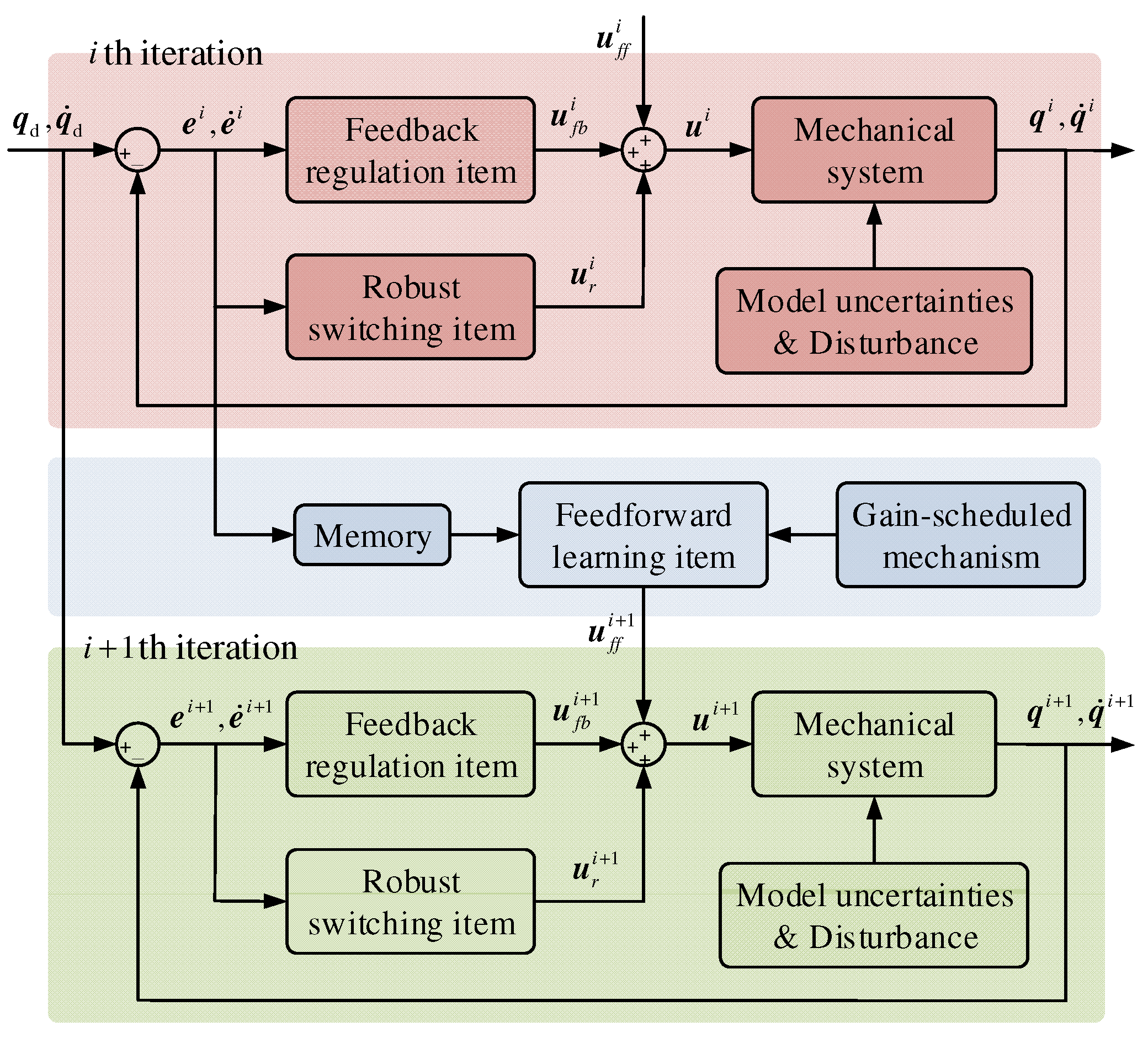
Figure 2.
Diagram of the two-link robot manipulator.

Figure 3.
Position tracking under the first five iterations.

Figure 4.
Velocity tracking under the first five iterations.

Figure 5.
Control torques under first five iterations.
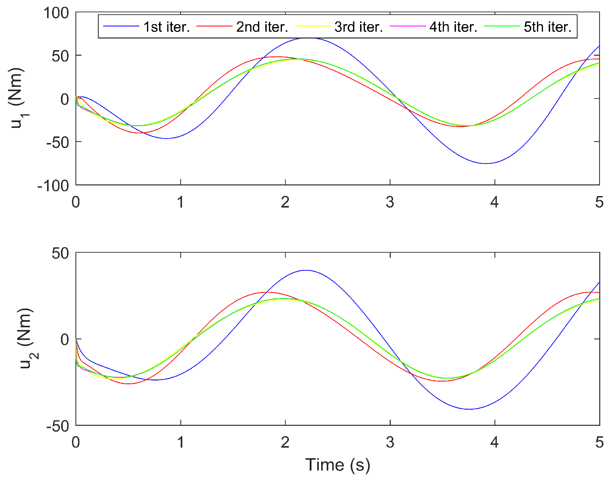
Figure 6.
MAEs of the position tracking under the first five iterations.

Figure 7.
MAEs of the velocity tracking under the first five iterations.
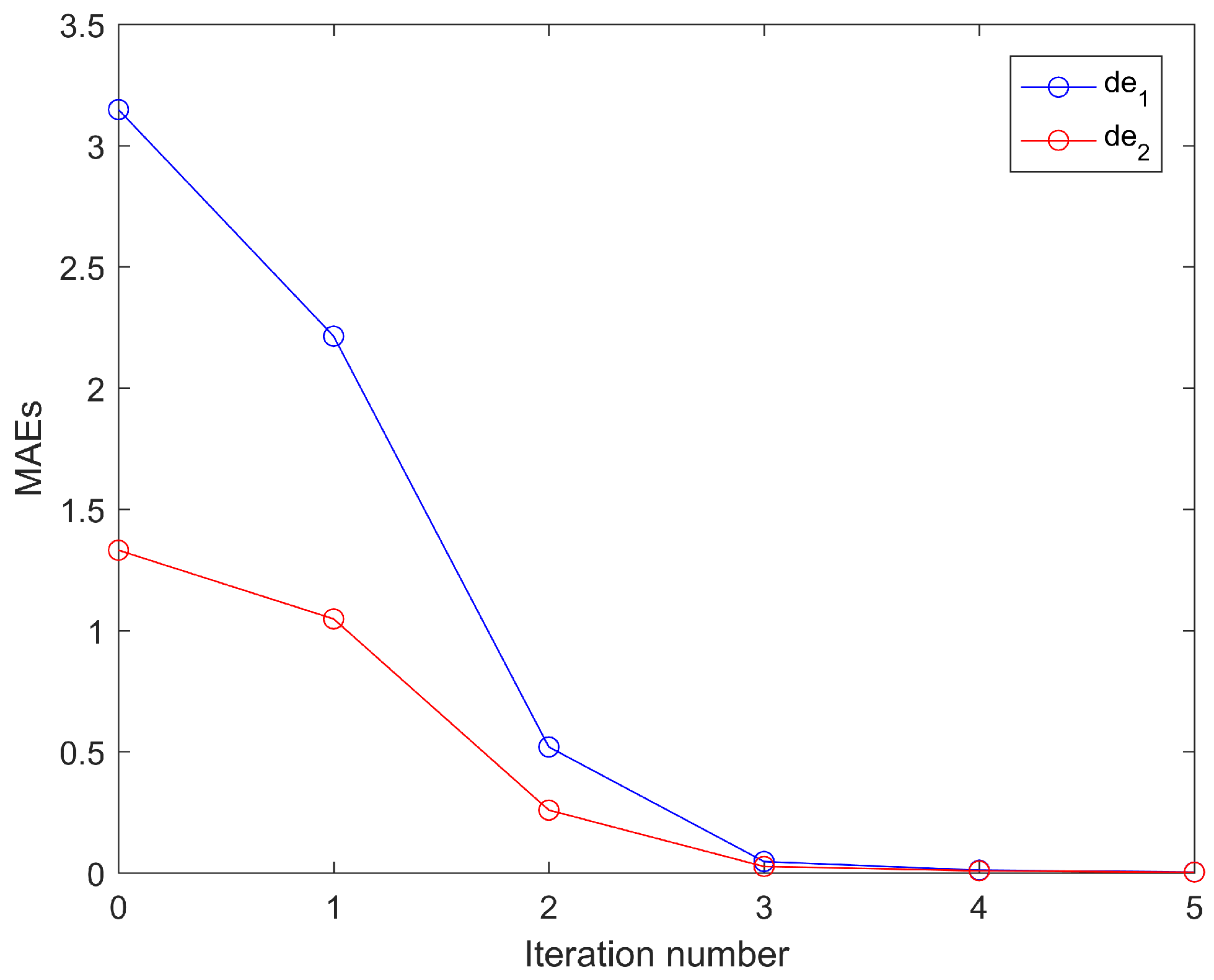
Figure 8.
Position tracking under both controllers.
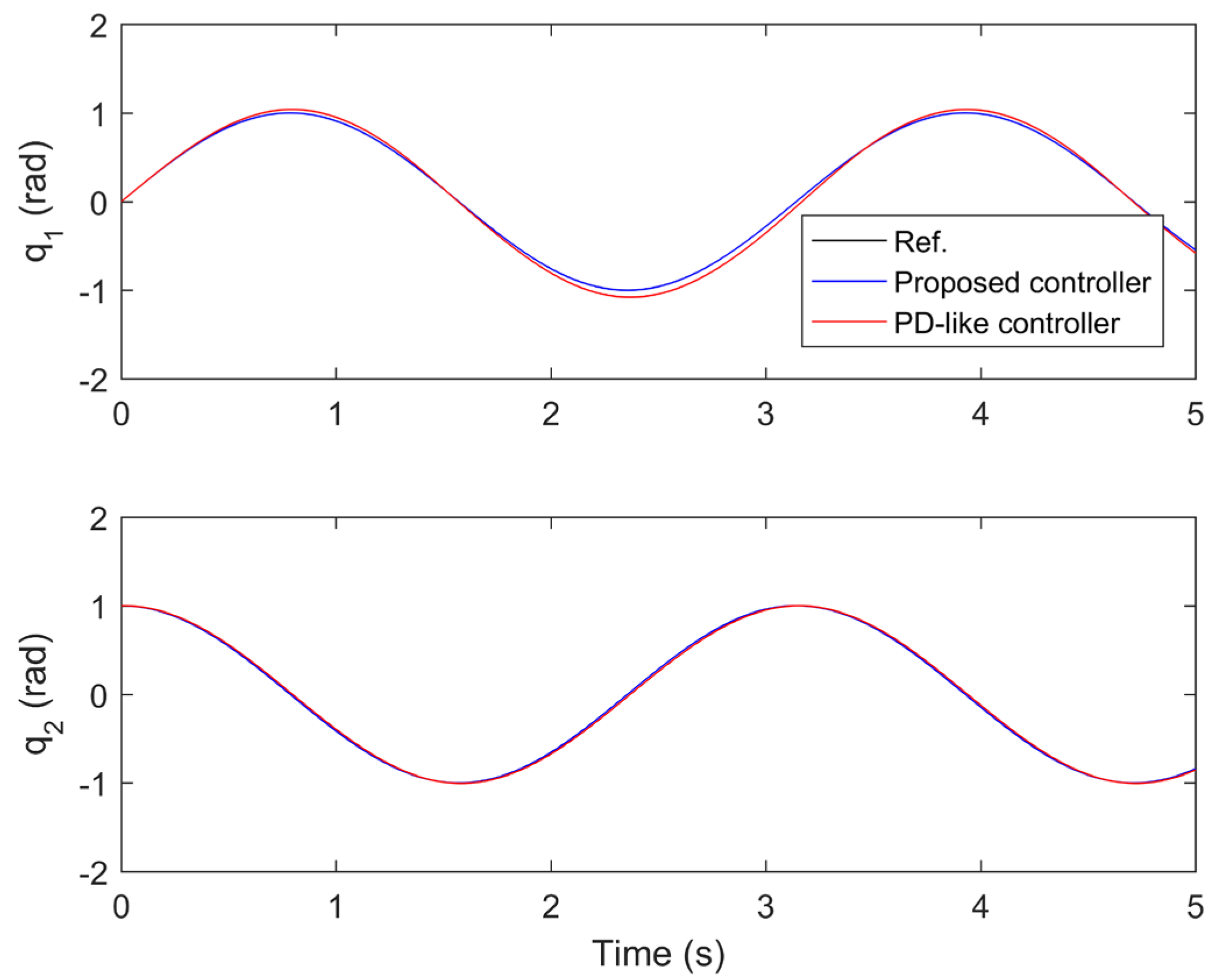
Figure 9.
Velocity tracking under both controllers.
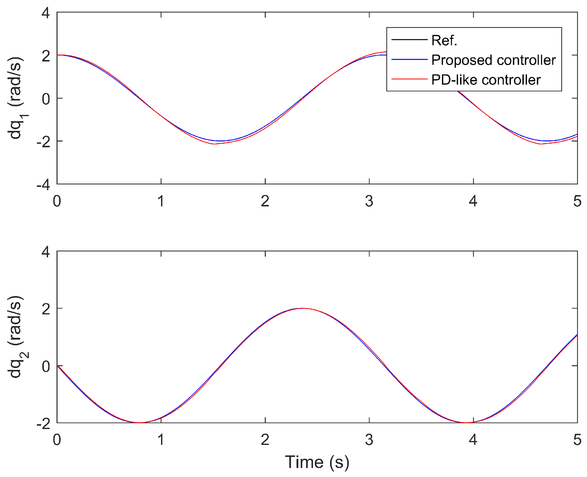
Figure 10.
Position tracking errors under both controllers.
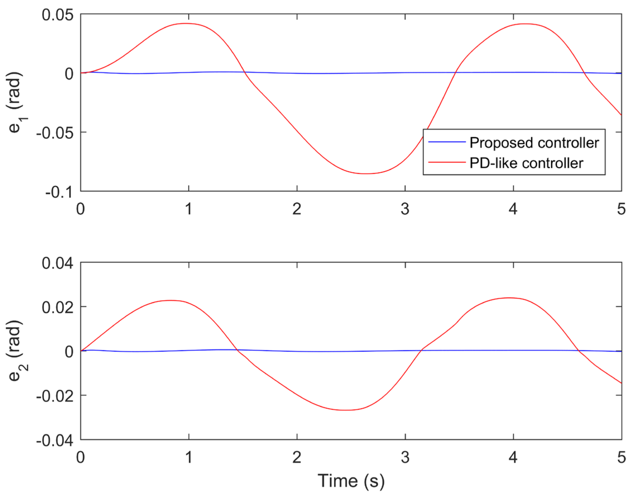
Figure 11.
Velocity tracking errors under both controllers.

Figure 12.
Control torques under both controllers.
Publisher’s Note: MDPI stays neutral with regard to jurisdictional claims in published maps and institutional affiliations. |
© 2022 by the authors. Licensee MDPI, Basel, Switzerland. This article is an open access article distributed under the terms and conditions of the Creative Commons Attribution (CC BY) license (https://creativecommons.org/licenses/by/4.0/).
Share and Cite
MDPI and ACS Style
Yao, Q.; Jahanshahi, H.; Bekiros, S.; Mihalache, S.F.; Alotaibi, N.D. Gain-Scheduled Sliding-Mode-Type Iterative Learning Control Design for Mechanical Systems. Mathematics 2022, 10, 3005. https://doi.org/10.3390/math10163005
AMA Style
Yao Q, Jahanshahi H, Bekiros S, Mihalache SF, Alotaibi ND. Gain-Scheduled Sliding-Mode-Type Iterative Learning Control Design for Mechanical Systems. Mathematics. 2022; 10(16):3005. https://doi.org/10.3390/math10163005
Chicago/Turabian StyleYao, Qijia, Hadi Jahanshahi, Stelios Bekiros, Sanda Florentina Mihalache, and Naif D. Alotaibi. 2022. "Gain-Scheduled Sliding-Mode-Type Iterative Learning Control Design for Mechanical Systems" Mathematics 10, no. 16: 3005. https://doi.org/10.3390/math10163005
Note that from the first issue of 2016, this journal uses article numbers instead of page numbers. See further details here.