Improved Nonfragile Sampled-Data Event-Triggered Control for the Exponential Synchronization of Delayed Complex Dynamical Networks

Abstract

The exponential synchronization of complex dynamical networks (CDNs) under improved nonfragile sampled-data event-triggered control (INFSDETC) is investigated in this study. A meaningful yet challenging issue is solved, namely, it can adjust the triggering mode and the triggering frequency to adapt to more situations in the event-triggered scheme in which it is able to adjust the triggering condition exponentially and linearly, and dynamically adjust the triggering according to the time and state. By using control theory and Lyapunov analysis theory, an improved event-triggered controller was constructed for more intelligent control and to ensure exponential synchronization for CDNs. Lastly, significant numerical simulation examples are developed to show the usefulness and the performance of the proposed methods.

1. Introduction

CDNs are network structures composed of complex network nodes whose synchronization performance drives network nodes to move or achieve the goal of coordination [1]. Complex network systems are widely used in biology, unmanned aerial vehicles, and power grids, and have received extensive attention [1,2,3,4]. The authors in [3,5] conducted pioneering studies on the synchronization of complex networks. There are many studies on the performance analysis of dynamical systems [4,6,7,8,9,10]. One of the important tasks in complex networks is to design a reasonable controller to allow for the system to achieve excellent performance. The event-triggered scheme was recently recognized to efficiently enable saving computing resources and handling control problems [11,12,13]. However, there are still many triggering and control problems to be solved in the event-triggered control of CDNs.

In order to explore the complex relationships of society and biology, researchers proposed the physical characteristics of higher-order interactions in complex networks in [2]. Exponential synchronization is an important performance index of complex networks to explore dynamical theory and dynamical features. The almost surely exponential synchronization for CDNs under noise signals was studied in [14]. The mean-square exponential synchronization for N linearly coupled complex networks, including Markovian switching and time delays, was investigated in [15]. In [16], exponential synchronization for a complex dynamical network containing coupling time delay and impulsive signals was studied. We explore the new exponential synchronization criteria of CDNs under a more general event-triggered controller. In several studies on the performance of CDNs, sampling technology was increasingly applied to the exponential synchronization problem of complex network systems. Sampled-data controllers are designed to achieve exponential synchronization for CDNs. Exponential synchronization for CDNs under sampled-data feedback control was studied in [17]. Nonfragile-memory sampled-data control was used for the exponential synchronization of delayed CDNs in [10]. In [18], the researchers gave new synchronization conditions with sampled-data control and a new integral inequality. Although there are extensive studies on the exponential synchronization of CDNs, there are few on the exponential synchronization of CDNs under INFSDETC, which needs to be further studied.

The event-triggered scheme (ETS) as an effective control method has attracted the interest of researchers due to its excellent monitoring control performance and resource-saving advantages. The working mechanism of the event-triggered scheme is to activate the triggering program to further control the system whenever the error between the current state of the concerned system and the previous one reaches a certain threshold [19,20]. A centralized and then distributed ETS was proposed in [21]: when the controller is updated, only the information of its neighbor nodes is needed. An ETC that is based on sampled-data signals was proposed in [22] and was further developed later. This does not require additional hardware to monitor the immediate status of the system in the sampled-data-based ETS. Due to the factors of communication and sensors, the controller in dynamical systems allows for the system to have infinite switching in a finite time. This phenomenon is called Zeno behavior or the Zeno phenomenon [23]. In event-triggered control, Zeno behavior is mainly represented by the case in which the trigger is activated infinitely in a finite time. Thus, Zeno behavior in this paper denotes infinite triggering behavior in finite time. The Zeno phenomenon was difficult to avoid for many systems with small perturbations in [24]. Therefore, the event-triggered scheme with sampled-data signals has become a common method. A recent overview of sampled-data event-triggered control was developed in [20]. To sum up the above, there are many studies on classical event-triggered protocols and common event-triggered schemes in various forms. However, setting the triggering threshold and error parameter needs to be further enriched to achieve more flexible triggering and match the environment of the system. The adjustment of the triggering mechanism needs to be further improved, such as via linear, exponential, and dynamic adjustments.

In this study, the event-triggered mechanism is improved to become a more general form and more adaptable to various system environments. New exponential convergence criteria for complex networks were obtained. The several contributions of this paper are listed below:

• Triggering Condition (4) is a generalized form covering situations in many other studies [25,26,27]. The trigger in the improved sampled-data event-triggered scheme was extended to be accelerated or decelerated linearly and exponentially, which increases the flexibility of the triggering scheme.
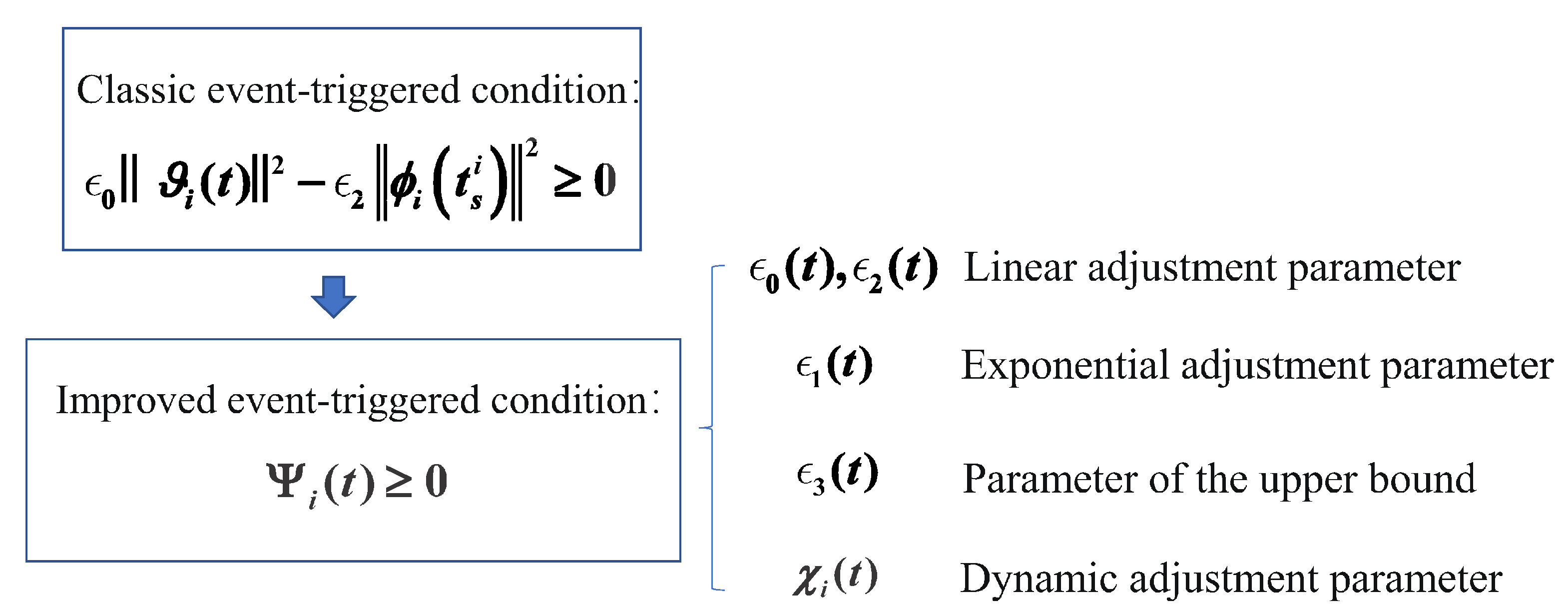
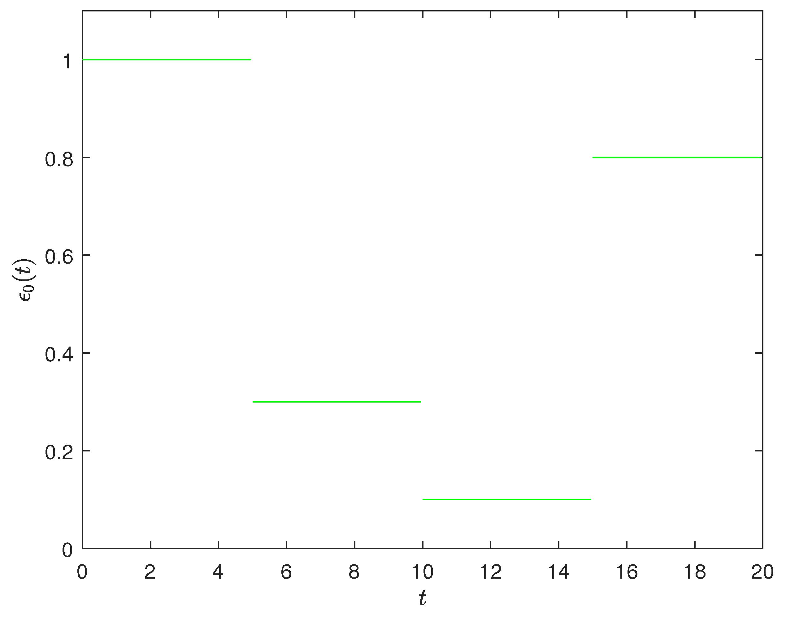
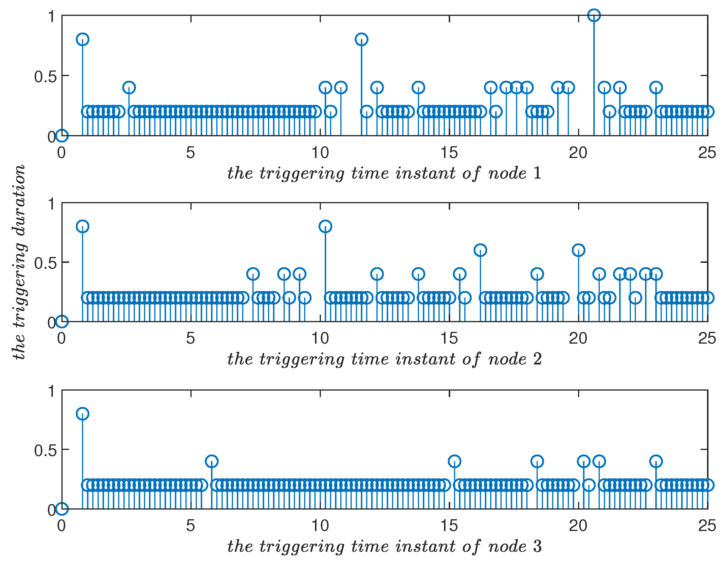
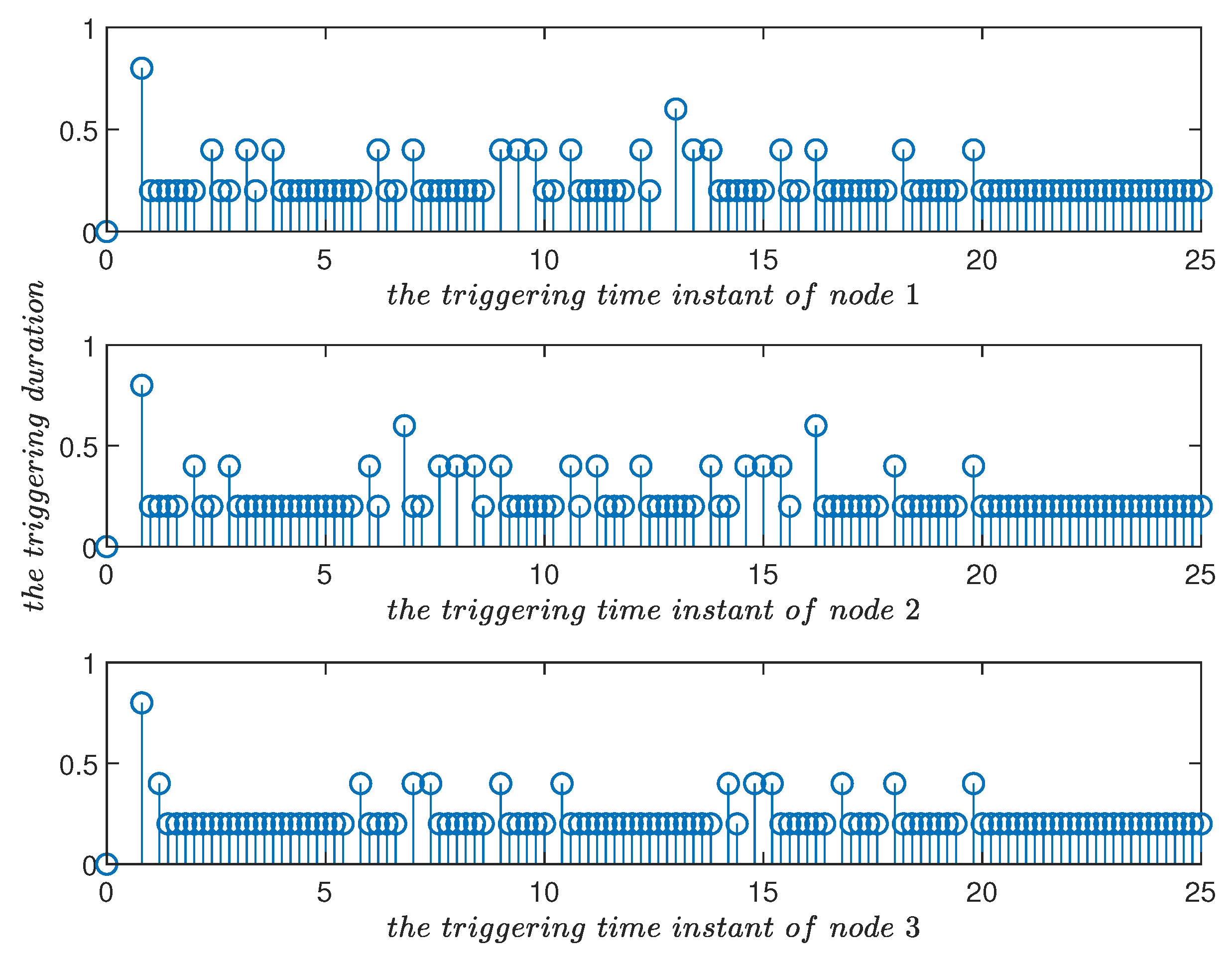
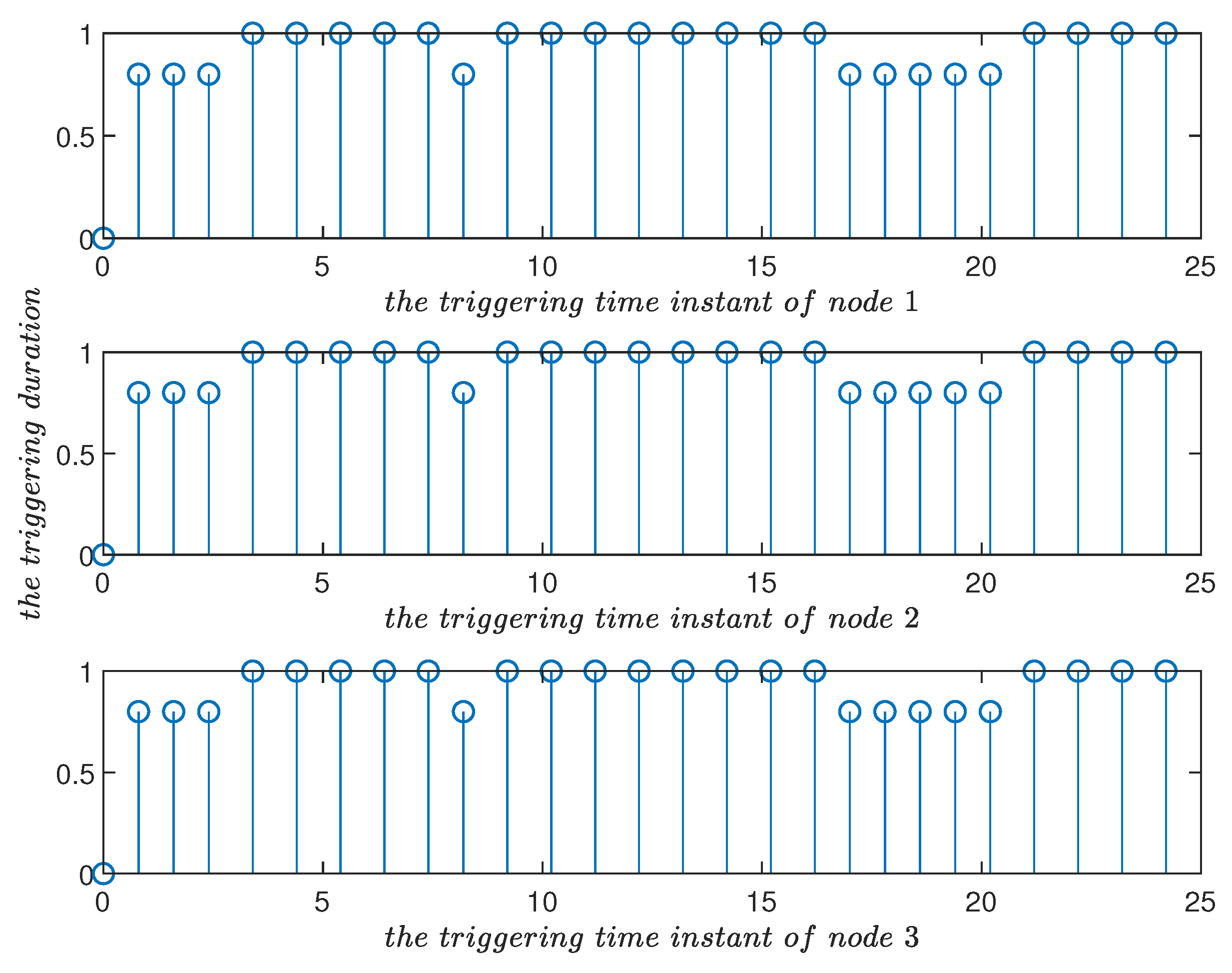
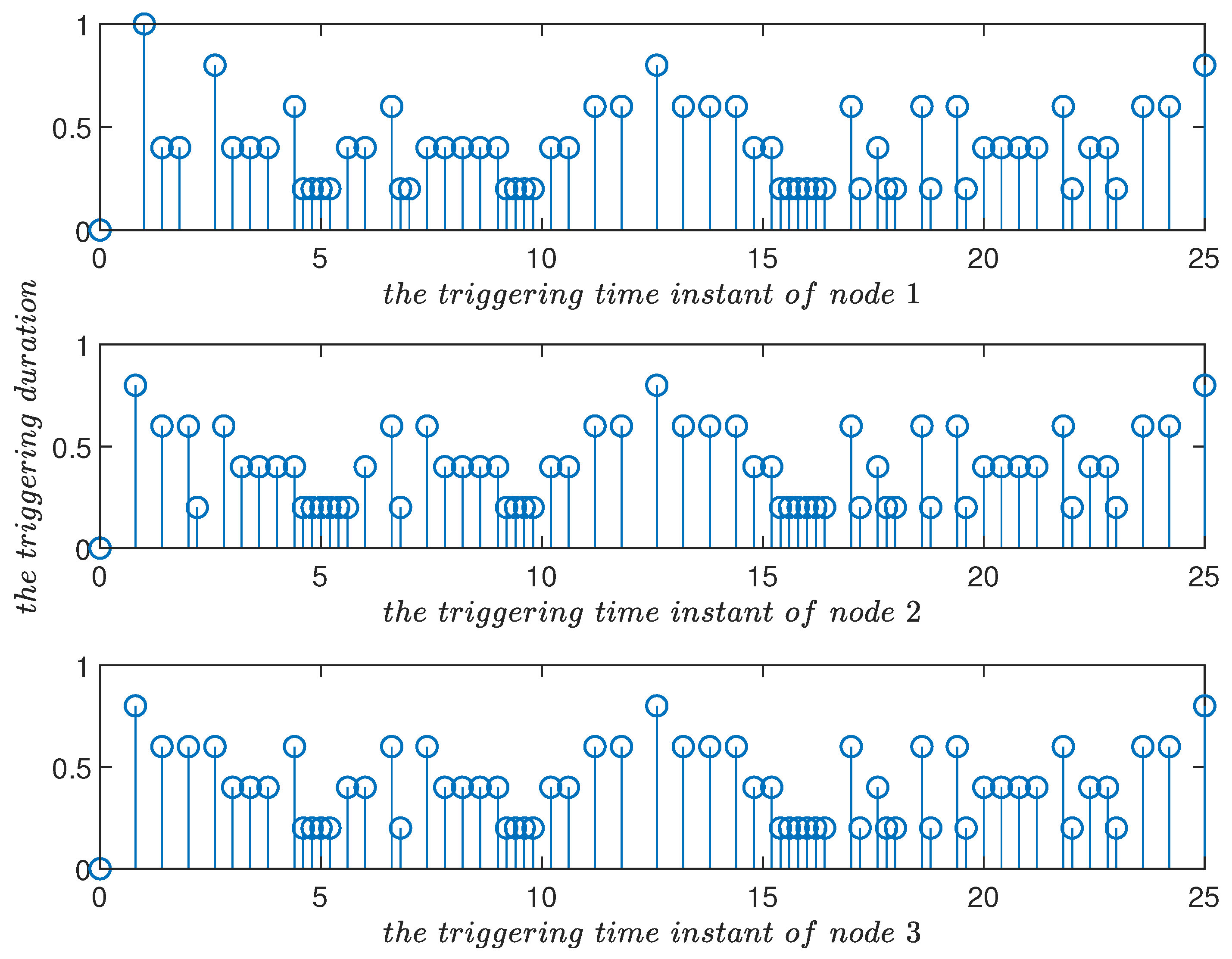
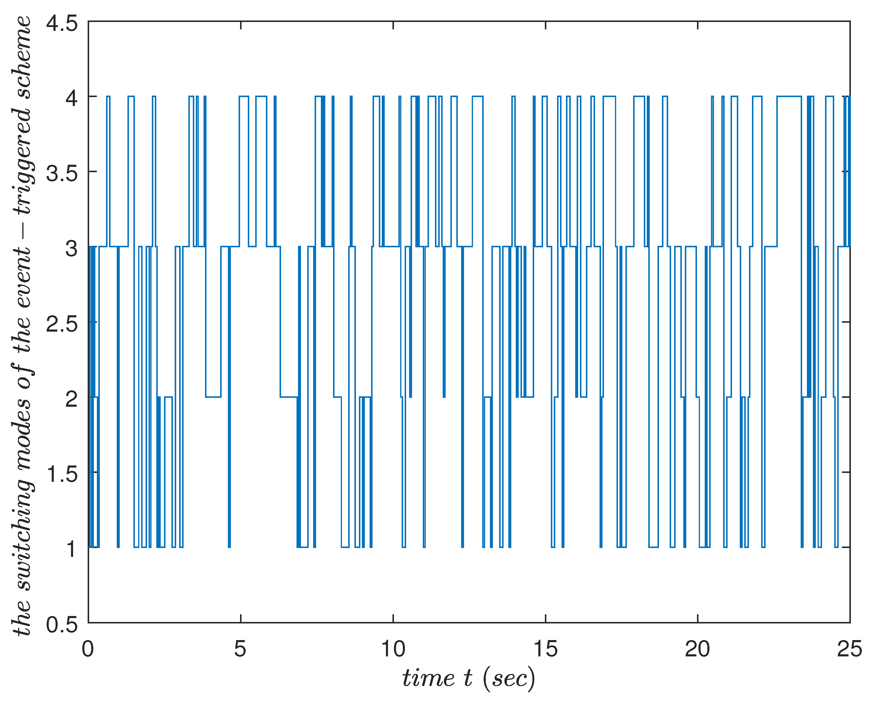
• The piecewise function was applied to the triggering condition in Remark 1, which can realize the flexibility of time according to the actual demand of different time periods. For the randomness of different triggering scenarios, Markov switching is applied to allow for the triggering condition to better adapt to possible scenarios, which is described in detail in Remark 1. The dynamic adjustment of the triggering is also realized in the event-triggered scheme described in Remark 3. Their results are given in the examples.
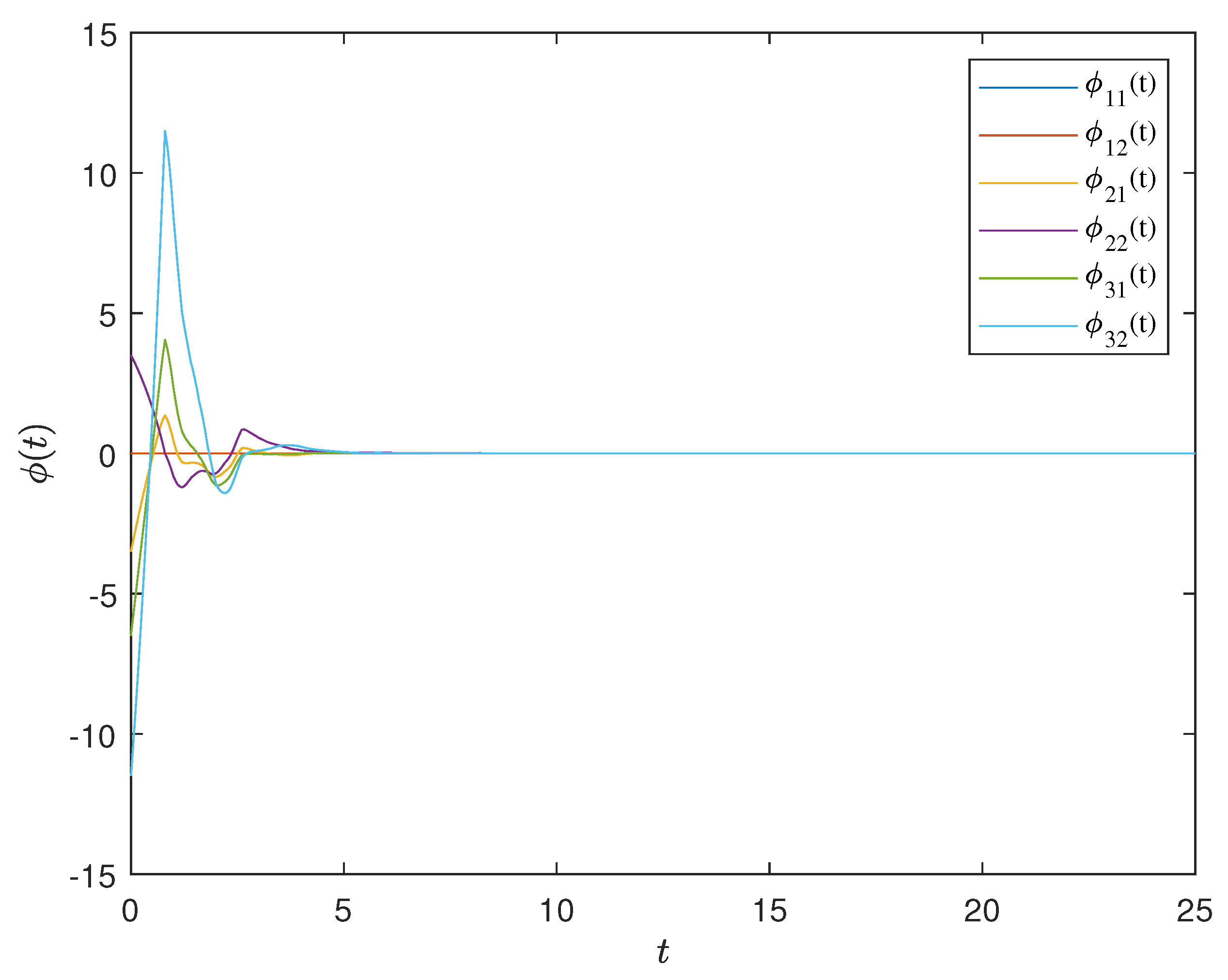
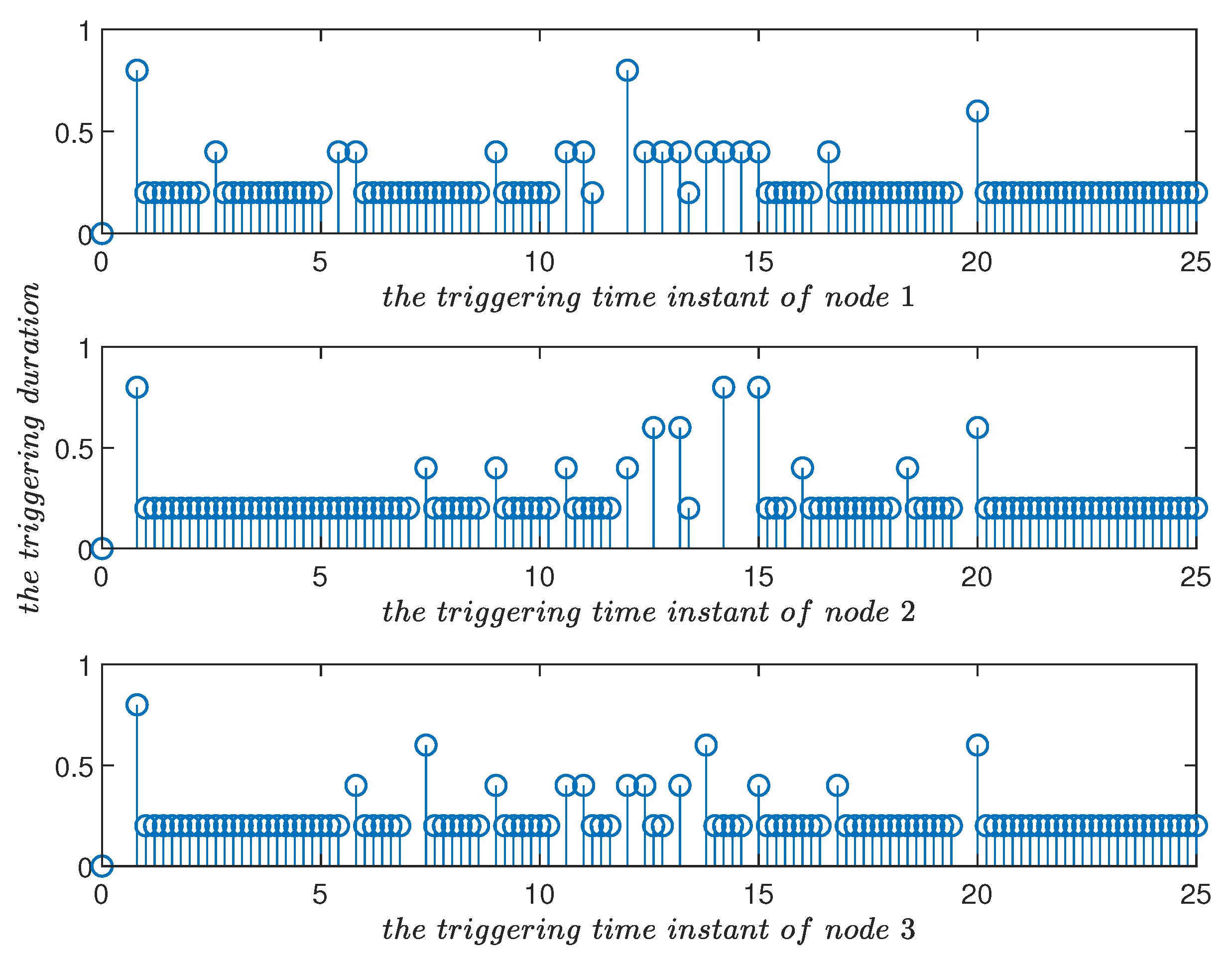
• The triggering time instants of different nodes were sequenced into the control time series. This rearrangement was well-handled and facilitated performance analysis of the system. Under the designed event-triggered control scheme, the nonfragile exponential synchronization criteria of complex networks are obtained.

Notations: Throughout the text, ${\mathbb{R}}^n$ and ${\mathbb{R}}^{n\times n}$ stand for n-dimensional Euclidean space and $n\times n$ real matrices, respectively. ${\mathbb{S}}^n$ is the set of all real $n\times n$ symmetric matrices. $sym\left\{X\right\}$ denotes $X+X^T$. For two symmetric matrices P and Q, inequality $P\ge Q$ ($P>Q$) denotes that matrix $P-Q$ is non-negative definite (positive definite). diag… means the block diagonal matrix. ∗ represents blocks of elements below the diagonal of a symmetric matrix. ⨂ stands for the Kronecker product operation of the matrices, and 0 represents zero or a zero matrix with appropriate dimension. $n\times N$ is denoted by $\mathbb{N}$. Prob… and E denote the probability of random variables and the operation of mathematical expectations, respectively. $I\_n=diag\underbrace{1,1,\cdots ,1}\_n$.

2. Preliminaries

Given CDNs containing a set of N nodes:

$${\dot{\phi }}_i\left(t\right)=g\left({\phi }_i\left(t\right)\right)+\gamma \sum _{j=1}^N{h}_{ij}A{\phi }_j(t-\tau \left(t\right))+u_i\left(t\right),$$

(1)

where ${\phi }_i\left(t\right)\in {\mathbb{R}}^n,i=1,2,\dots ,N,$ denotes the i-th node’s state vector and ${\phi }_i\left(t\right)=[{\phi }_{i1}\left(t\right),{\phi }_{i2}(t$$),\dots ,{\phi }_{in}{\left(t\right)]}^T$. Matrix $H={\left(h_{ij}\right)}_{NN}$ and the scalar $\gamma$ stand for the out-coupled configuration matrix and the coupling strength, respectively. $A=diag\{a_1,a_2,\dots ,a_n\}$ is a known non-negative diagonal matrix. Here, $h_{ii}$ is denoted by $h_{ii}=-{\sum }_{j=1,j\ne i}^N{h}_{ij},i=1,2,\dots ,N$. $h_{ij}>0$ means that node i is linked to node $j(i\ne j)$; if not, then $h_{ij}=0$. $\tau \left(t\right)$, satisfying $0\le \tau \left(t\right)\le \tau$ and $\dot{\tau }\left(t\right)\le \mu$ means time-varying delays where $\mu$ and $\tau$ are known scalars. $u_i\left(t\right)$ represents the control input. Let variable $Ꮗ\left(t\right)\in {\mathbb{R}}^n$ be the state vector of the unforced node and let it satisfy $\dot{Ꮗ}\left(t\right)=g\left(Ꮗ\left(t\right)\right)$. $g(·)$$:{\mathbb{R}}^n\mapsto {\mathbb{R}}^n$ is the continuous and bounded nonlinear activation function that satisfies the inequality as follows:

$${[g\left({\varphi }_i\right)-g\left({\varphi }_j\right)-{\daleth }_1({\varphi }_i-{\varphi }_j)]}^T[g\left({\varphi }_i\right)-g\left({\varphi }_j\right)-{\daleth }_2({\varphi }_i-{\varphi }_j)]\le 0,\forall {\varphi }_i,{\varphi }_j\in {\mathbb{R}}^n,$$

(2)

where ${\daleth }_1$, ${\daleth }_2\in {\mathbb{R}}^{n\times n}$ are known matrices.

Let ${\varphi }_i\left(t\right)={\phi }_i\left(t\right)-Ꮗ\left(t\right)$; the following dynamic system from CDNs (1) and $\dot{Ꮗ}\left(t\right)=g\left(Ꮗ\left(t\right)\right)$ can be deduced:

$${\dot{\varphi }}_i\left(t\right)=f\left({\varphi }_i\left(t\right)\right)+\gamma \sum _{j=1}^N{h}_{ij}A{\varphi }_j(t-\tau \left(t\right))+u_i\left(t\right),$$

(3)

where $f\left({\varphi }_i\left(t\right)\right)=g\left({\phi }_i\left(t\right)\right)-g\left(Ꮗ\left(t\right)\right)$, $i=1,2,\dots ,N$.

The minimal sampling time interval in controller was set to be h. The control time instant of the controller $u_i\left(t\right)$ is defined as $t_s^i$, which was determined with the following conditions of the improved sampled-data event-triggered scheme in order to achieve the more flexible and intelligent error detection of the system (3).

$${\displaystyle t_{s+1}^i=t_s^i+inf\{\kappa h:t>t_s^i,{\mathrm{\Psi }}_i\left(t\right)\ge 0\},s=1,2,\cdots ,\infty ,\kappa =1,2,\cdots ,\infty ,}$$

(4)

where

$${\mathrm{\Psi }}_i\left(t\right)=\left({ϵ}_0\left(t\right){\parallel {\vartheta }_i\left(t\right)\parallel }^2{e}^{{ϵ}_1\left(t\right)(t-t_s^i)}-{ϵ}_2\left(t\right){∥{\varphi }_i\left(t_s^i\right)∥}^2-{\chi }_i\left(t\right)\right)\left(1-\frac{t-t_s^i}{{ϵ}_3}\right),$$

$${ϵ}_0\left(t\right)\in [\underline{{ϵ}_0},\overline{{ϵ}_0}],{ϵ}_1\left(t\right)\in [\underline{{ϵ}_1},\overline{{ϵ}_1}],{ϵ}_2\left(t\right)\in [\underline{{ϵ}_2},\overline{{ϵ}_2}],$$

$${\dot{\chi }}_i\left(t\right)={ϵ}_4{\chi }_i\left(t\right)+{ϵ}_5\left({ϵ}_0\left(t\right){\parallel {\vartheta }_i\left(t\right)\parallel }^2{e}^{{ϵ}_1\left(t\right)(t-t_s^i)}-{ϵ}_2\left(t\right){∥{\varphi }_i\left(t_s^i\right)∥}^2\right),$$

$${\vartheta }_i\left(t\right)={\varphi }_i\left(t\right)-{\varphi }_i\left(t_s^i\right),$$

with $0\le \underline{{ϵ}_0}\le \overline{{ϵ}_0},0\le \underline{{ϵ}_1}\le \overline{{ϵ}_1},0\le \underline{{ϵ}_2}\le \overline{{ϵ}_2},{ϵ}_3>0,{ϵ}_4\ge 0,{ϵ}_5\ge 0$, $t_0^i=0$, ${\chi }_i\left(t_0^i\right)\ge 0$. Obviously, no Zeno behavior occurred under the event-triggered scheme, since h was the minimal triggering time instant interval. From the condition, it can be deduced that $\hslash \triangleq sup\left\{t_{s+1}^i-t_s^i\right\}=\left(1+\left[\frac{{ϵ}_3}{h}\right]\right)h$. The explanations of the desired event-triggered scheme are shown in Figure 1 and the following remarks.

Remark 1.

${ϵ}_0\left(t\right)$,${ϵ}_1\left(t\right)$ and ${ϵ}_2\left(t\right)$ are bounded functions where the numerical change of the function can be reflected on the triggering frequency and triggering state. The corresponding needed function can be set according to the timing to increase or decrease the triggering frequency exponentially or linearly. In particular, taking ${ϵ}_0\left(t\right)$,${ϵ}_1\left(t\right)$ and ${ϵ}_2\left(t\right)$ as piecewise functions or switching functions, the triggering mechanism has the following advantages shown in Cases 1 and 2.

Case 1: As ${ϵ}_0\left(t\right)$,${ϵ}_1\left(t\right)$ and ${ϵ}_2\left(t\right)$ were set to be piecewise functions, different triggering conditions could be used in different time periods, reflecting the different trigger characteristics in multiple time periods and adapting to the environment in multiple time periods.

Case 2: As ${ϵ}_0\left(t\right),{ϵ}_1\left(t\right),{ϵ}_2\left(t\right)$ become ${ϵ}_0^{\varrho \left(t\right)}\left(t\right),{ϵ}_1^{\varrho \left(t\right)}\left(t\right),{ϵ}_2^{\varrho \left(t\right)}\left(t\right)$, respectively, where $\varrho \left(t\right)$ is the Markov switching function described as [28,29], the triggering condition changed into the switching mode form. That is, ${ϵ}_0\left(t\right),{ϵ}_1\left(t\right),{ϵ}_2\left(t\right)$ were able to be in the different mode based on $\varrho \left(t\right)$ shown in Figure 2, causing the switching condition to be in different working modes. At this point, if the system also contains switching modes, and triggering conditions can be well-matched with the system’s modes.

Remark 2.

${\varphi }_i\left(t\right)$ is dependent on ${\displaystyle \sum _{j=1}^N}{h}_{ij}A{\varphi }_j(t-\tau \left(t\right))$; there is a coupling term ${\displaystyle \sum _{j=1}^N}{h}_{ij}A{\varphi }_j(t-\tau \left(t\right))$. Therefore, there are coupling terms implicitly for event-triggering parameters that include the communicating characteristics of network nodes with each other. The parameters in the event-triggered scheme are related to the coupling node related to j, and are implicitly in a coupling form that could instantly reflect the data errors between nodes, which in turn facilitates more timely control.

Remark 3.

Dynamic variable ${\chi }_i\left(t\right)$ dynamically expands the triggering threshold to increase the flexibility of the triggered scheme. When the system gradually stabilizes, the triggered mechanism is activated only when the dynamically expanded threshold is reached, which reduces the waste of communication resources to a certain extent. If it is not necessary to activate dynamic variable ${\chi }_i\left(t\right)$, setting ${ϵ}_4={ϵ}_5=0$ would be satisfied.

Remark 4.

To increase the flexibility of the event-triggered mechanism, parameters ${ϵ}_0\left(t\right)$, ${ϵ}_1\left(t\right)$, ${ϵ}_2\left(t\right)$, ${ϵ}_3$, ${ϵ}_4$, ${ϵ}_5$ were set to adjust the trigger from a different direction in combination with exponential and linear functions. When the triggering frequency needs to be linearly changed, ${ϵ}_0\left(t\right)$ and ${ϵ}_2\left(t\right)$ can be used as adjusting functions; then, the trend of the triggering function ${\mathrm{\Psi }}_i\left(t\right)$ generally changes linearly. ${ϵ}_2\left(t\right)$ plays an important role as an exponential adjusting parameter in the process of acceleration or deceleration of triggering times when an exponential change in triggering frequency is required. $1-\frac{t-t_s^i}{{ϵ}_3}$ is used as an upper bound function for the triggering scheme, aiming to avoid no triggering time within a long time or to set artificially triggering upper bound. In this case, one can easily calculate an upper bound of triggering: $\left(1+\left[\frac{{ϵ}_3}{h}\right]\right)h$. If there is no need for the upper bound, ${ϵ}_3$ could be set to a very large number to meet the demands.

The control time instants were set to be ${\left\{t_s^i\right\}}_{s=1}^{+\infty }$. Further, time instants ${\left\{t_k\right\}}_{k=1}^{+\infty }$ were introduced to rewrite System (3) as System (7) in compact form. The control input $u_i\left(t\right)$ of node i is shown below:

$$\begin{array}{cc}\hfill u_i\left(t\right)& =(K_{1i}+\delta \left(t\right)\mathrm{\Delta }{K}_{1i}\left(t\right)){\varphi }_i\left(t_s^i\right)+(K_{2i}+\delta \left(t\right)\mathrm{\Delta }{K}_{2i}\left(t\right)){\varphi }_i(t_s^i-ı)\hfill \\ & =(K_{1i}+\delta \left(t\right)\mathrm{\Delta }{K}_{1i}\left(t\right)){\theta }_i\left(t_k\right){\varphi }_i\left(t_k\right)+(K_{2i}+\delta \left(t\right)\mathrm{\Delta }{K}_{2i}\left(t\right)){\theta }_i\left(t_k\right){\varphi }_i(t_k-ı),t_k\le t<t_{k+1},\hfill \end{array}$$

(5)

with

$${\theta }_i\left(t_k\right)=\left\{\begin{array}{c}1,\mathrm{if}{t}_k=t_s^i;\hfill \\ 0,\mathrm{otherwise},\hfill \end{array}\right.$$

(6)

$$[\mathrm{\Delta }{K}_{1i}\left(t\right),\mathrm{\Delta }{K}_{2i}\left(t\right)]={\mathcal{H}}_i{\mathcal{P}}_i\left(t\right)[{\mathcal{E}}_{1i},{\mathcal{E}}_{2i}],$$

$${\mathcal{P}}_i^T\left(t\right){\mathcal{P}}_i\left(t\right)\le I,$$

$$Prob\left\{\delta \right(t)=1\}=\delta ,Prob\left\{\delta \right(t)=0\}=1-\delta ,$$

$$\mathcal{E}\{\delta \left(t\right)-\delta \}=0,\mathcal{E}\{{(\delta \left(t\right)-\delta )}^2\}=\delta (1-\delta ),$$

where matrices $K_{1i}$ and $K_{2i}$ are the controller gains that need to be determined. Matrices $\mathrm{\Delta }{K}_{1i}\left(t\right)$ and $\mathrm{\Delta }{K}_{2i}\left(t\right)$ stand for the interference signal of controller gain (ISCG). $\delta \left(t\right)$, obeying Bernoulli distribution, denotes the stochastic variable that is used to simulate the random occurrence of interference signals. If ISCG occurs, $\delta \left(t\right)=1$; otherwise, $\delta \left(t\right)=0$. Constant ı represents time delays occurring in the transmission of signals. The triggering time instants are reordered into the time instants of the controller, which can improve the degree of freedom of triggering conditions and the performance analysis of dynamical systems due to the weakening of triggering time instants (See Figure 3).

System (3) can be further rewritten as the following compact form using the Kronecker product:

$$\dot{\varphi }\left(t\right)=F\left(\varphi \left(t\right)\right)+\gamma (H\otimes A)\varphi (t-\tau \left(t\right))+K_1(\mathrm{\Theta }\left(t_k\right)\otimes I_n)\varphi \left(t_k\right)+K_2(\mathrm{\Theta }\left(t_k\right)\otimes I_n)\varphi (t_k-ı)+\delta \mathcal{H}p\left(t\right)-(\delta -\delta \left(t\right))\mathcal{H}p\left(t\right),$$

(7)

where

$$\begin{array}{cc}\hfill & F\left(\varphi \left(t\right)\right)={[f^T\left({\varphi }_1\left(t\right)\right),f^T\left({\varphi }_2\left(t\right)\right),\dots ,f^T\left({\varphi }_N\left(t\right)\right)]}^T,\hfill \\ \hfill & \varphi (·)={[{\varphi }_1^T(·),{\varphi }_2^T(·),\dots ,{\varphi }_N^T(·)]}^T,\hfill \\ \hfill & K_1=diag\{K_{11},K_{12},\dots ,K_{1N}\},\hfill \\ \hfill & K_2=diag\{K_{21},K_{22},\dots ,K_{2N}\},\hfill \\ \hfill & \mathrm{\Theta }\left(t_k\right)=diag\{{\theta }_1\left(t_k\right),{\theta }_2\left(t_k\right),\dots ,{\theta }_N\left(t_k\right)\},\hfill \\ \hfill & \mathcal{H}=diag\{{\mathcal{H}}_1,{\mathcal{H}}_2,\cdots ,{\mathcal{H}}_N\},\hfill \\ \hfill & \mathcal{P}\left(t\right)=diag\{{\mathcal{P}}_1\left(t\right),{\mathcal{P}}_2\left(t\right),\cdots ,{\mathcal{P}}_N\left(t\right)\},\hfill \\ \hfill & {\mathcal{E}}_1=diag\{{\mathcal{E}}_{11},{\mathcal{E}}_{12},\cdots ,{\mathcal{E}}_{1N}\},\hfill \\ \hfill & {\mathcal{E}}_2=diag\{{\mathcal{E}}_{21},{\mathcal{E}}_{22},\cdots ,{\mathcal{E}}_{2N}\},\hfill \\ \hfill & p\left(t\right)=\mathcal{P}\left(t\right)({\mathcal{E}}_1\varphi \left(t_k\right)+{\mathcal{E}}_2\varphi (t_k-ı)).\hfill \end{array}$$

Remark 5.

An interference signal is inevitable in the signal communication domain and its applications. The influence of interference signals on a dynamic system should be considered when a control input is designed. Since ISCG occurs randomly, variable $\delta \left(t\right)$ was designed to simulate this random process. Moreover, as the time delays in signal and information transmission happens occasionally, term ı was designed to describe more details in the controller. Control input $u_i\left(t\right)$ involves the information of two time instants: the sampling instant and its delayed instant, in which more information is integrated to render the running of the controller more precise.

Definition 1

([30]). If Error Dynamics (7) is exponentially stable, CDNs (1) are exponentially synchronized, i.e., there exist two scalars $\alpha ,\iota >0$, such that

$${\displaystyle \parallel \varphi \left(t\right)\parallel \le \iota e^{-\alpha t}\underset{-\nu \le \theta \le 0}{sup}\{\parallel \varphi \left(\theta \right)\parallel ,\parallel \dot{\varphi }\left(\theta \right)\parallel \},}$$

(8)

where ${\displaystyle \nu =max\{\tau ,\hslash \}}$, α denotes the decay rate, and ι denotes the decay coefficient.

Lemma 1

([31]). Given matrix $M>0$, in any continuously differentiable function $z\left(t\right):[a,b]⟼{\mathbb{R}}^{\mathbb{N}}$, the following inequality holds:

$${\int }_a^b{\stackrel{.}{z}}^T\left(\alpha \right)M\stackrel{.}{z}\left(\alpha \right)d\alpha \ge \frac{1}{b-a}{\zeta }_1^{T}M{\zeta }_1+\frac{3}{b-a}{\zeta }_2^{T}M{\zeta }_2,$$

where ${\zeta }_1=z\left(b\right)-z\left(a\right),{\zeta }_2=z\left(b\right)+z\left(a\right)-\frac{2}{b-a}{\int }_a^{b}z\left(\alpha \right)d\alpha$.

Lemma 2

([32]). Let $z\left(t\right):[a,\mathit{b})\to {\mathbb{R}}^{\mathbb{N}}$ and $z\left(a\right)=0$, such that the concerned integrations are well-defined. Then, for any positive matrix $M\in {\mathbb{R}}^{\mathbb{N}\times \mathbb{N}}$, the following inequality holds:

$${\int }_a^b{z}^{\mathrm{T}}\left(\alpha \right)Mz\left(\alpha \right)d\alpha \le \frac{4{(b-a)}^2}{{\pi }^2}{\int }_a^b{\dot{z}}^{\mathrm{T}}\left(\alpha \right)M\dot{z}\left(\alpha \right)d\alpha .$$

(9)

Lemma 3

([33]). For any matrix $\begin{array}{c}\hfill \left[\begin{array}{cc}{M}_1& S\\ *& M_2\end{array}\right]\end{array}$$\ge 0$, scalars $\tau >0,\tau \left(t\right)$ satisfying $0\le \tau \left(t\right)\le \tau$, and vector function $\dot{\phi }\left(t\right)$: $[-\tau ,0]\to {\mathbb{R}}^{\mathbb{N}}$, such that the concerned integrations are well-defined,

$${\displaystyle -\tau {\int }_{t-\tau \left(t\right)}^t\dot{\phi }{\left(\alpha \right)}^{\mathrm{T}}{M}_1\dot{\phi }\left(\alpha \right)\mathrm{d}\alpha -\tau {\int }_{t-\tau }^{t-\tau \left(t\right)}\dot{\phi }{\left(\alpha \right)}^{\mathrm{T}}{M}_2\dot{\phi }\left(\alpha \right)d\alpha \le \aleph {\left(t\right)}^{\mathrm{T}}\mathrm{\Omega }\aleph \left(t\right),}$$

(10)

where

$$\aleph \left(t\right)={[\phi {\left(t\right)}^{\mathrm{T}},\phi {(t-\tau \left(t\right))}^{\mathrm{T}},\phi {(t-\tau )}^{\mathrm{T}}]}^{\mathrm{T}},$$

$$\mathrm{\Omega }=\left[\begin{array}{ccc}-M_1& M_1-S& S\\ *& -M_1-M_2+sym\left\{S\right\}& -S+M_2\\ *& *& -M_2\end{array}\right].$$

3. Main Results

In this section, under INFSDETC, the exponential synchronization criteria of System (7) are obtained.

Theorem 1.

Given scalars $\theta \ge 0$, ${\epsilon }_1\ge 0$, ${\epsilon }_2\ge 0$, $h>0$, $0\le \underline{{ϵ}_0}\le \overline{{ϵ}_0},0\le \underline{{ϵ}_1}\le \overline{{ϵ}_1},0\le \underline{{ϵ}_2}\le \overline{{ϵ}_2},{ϵ}_3>0,{ϵ}_4\ge 0,{ϵ}_5\ge 0$, $h\ge 0$, $\mu \ge 0$, $\tau \ge 0$, $ı>0$, ${\kappa }_1$, ${\kappa }_2$, ${\kappa }_3$, ${\kappa }_4$, and matrices $\mathcal{H}=diag\{{\mathcal{H}}_1,{\mathcal{H}}_2,\cdots ,{\mathcal{H}}_N\}$, ${\mathcal{E}}_1=diag\{{\mathcal{E}}_{11},{\mathcal{E}}_{12},\cdots ,{\mathcal{E}}_{1N}\}$, ${\mathcal{E}}_2=diag\{{\mathcal{E}}_{21},{\mathcal{E}}_{22},\cdots ,{\mathcal{E}}_{2N}\}$, Error System (7) achieves globally exponential stability with INFSDETC (5) if there exist symmetric positive definite matrices P∈${\mathbb{R}}^{3\mathbb{N}\times 3\mathbb{N}}$, $Q_1$, $Q_2$, $M_1$, $M_2$, $M_3$∈${\mathbb{R}}^{\mathbb{N}\times \mathbb{N}}$, $N_1$=$\begin{array}{c}\hfill \left[\begin{array}{ccc}{N}_{111}& N_{112}\ast & N_{122}\end{array}\right]\end{array}$∈${\mathbb{R}}^{\mathbb{N}\times \mathbb{N}}$, $N_2$=$\begin{array}{c}\hfill \left[\begin{array}{cc}{N}_{211}& N_{212}\\ *& N_{222}\end{array}\right]\end{array}$∈${\mathbb{R}}^{\mathbb{N}\times \mathbb{N}}$, U∈${\mathbb{R}}^{\mathbb{N}\times \mathbb{N}}$, $Z_1$=$\begin{array}{c}\hfill \left[\begin{array}{ccc}{Z}_{111}& Z_{112}& Z_{113}\\ *& Z_{122}& Z_{123}\\ *& *& Z_{133}\end{array}\right]\end{array}$∈${\mathbb{R}}^{3\mathbb{N}\times 3\mathbb{N}}$, $Z_2$∈${\mathbb{R}}^{\mathbb{N}\times \mathbb{N}}$, $X_3$, $X_4$∈${\mathbb{R}}^{\mathbb{N}\times \mathbb{N}}$, $S=diag\{S_1,S_2,\dots ,S_N\}$, $W_1=diag\{W_{11},W_{12},\dots ,W_{1N}\}$, $W_2=diag\{W_{21},$$W_{22},\dots ,W_{2N}\}$∈${\mathbb{R}}^{\mathbb{N}\times \mathbb{N}}$, any matrices $X_1$, $X_2$∈${\mathbb{R}}^{\mathbb{N}\times 10\mathbb{N}}$, Y∈${\mathbb{R}}^{\mathbb{N}\times \mathbb{N}}$, such that the following linear matrix inequalities hold:

$$\left[\begin{array}{cccc}{\Lambda }_1+\hslash {\Lambda }_2& \frac{\hslash }{2}{\overline{Z}}_1& \sqrt{\hslash }{X}_1^T& 3\sqrt{\hslash }{X}_2^T\\ *& -X_3& 0& 0\\ *& *& -e^{2\theta \hslash }{N}_{222}& 0\\ *& *& *& -3e^{2\theta \hslash }{N}_{222}\end{array}\right]<0,$$

(11)

$$\left[\begin{array}{ccc}{\Lambda }_1+\hslash {\Lambda }_3& \frac{\hslash }{2}{\overline{Z}}_1& {϶}_1^T{Z}_2\\ *& -X_3& 0\\ *& *& -X_4\end{array}\right]<0,$$

(12)

$$\left[\begin{array}{cc}{e}^{-2\theta \tau }{M}_1+(1-\mu )e^{-2\theta ϵ}{M}_2& Y\\ *& e^{-2\theta \tau }{M}_1\end{array}\right]\ge 0,$$

(13)

where the relevant mathematical symbols and equations are listed in Appendix A.

Moreover, the control gain matrices are determined with

$$K_{1i}=S_i^{-1}{W}_{1i},K_{2i}=S_i^{-1}{W}_{2i},i=1,2,\cdots ,N.$$

(14)

Proof of Theorem 1.

The Lyapunov functional is defined as follows:

$$V(t,t_k)=\sum _{l=1}^7{V}_l(t,t_k),t\in [t_k,t_{k+1}),$$

(15)

where

$$\begin{array}{cc}\hfill & V_1(t,t_k)=(t-t_k)e^{2\theta t}{\eta }^T\left(t\right)P\eta \left(t\right)\hfill \\ \hfill & V_2(t,t_k)=e^{2\theta \tau }{\int }_{t-\tau \left(t\right)}^t{e}^{2\theta s}{\varphi }^T\left(s\right)Q_1\varphi \left(s\right)ds+e^{2\theta \tau }{\int }_{t-\tau }^t{e}^{2\theta s}{\varphi }^T\left(s\right)Q_2\varphi \left(s\right)ds,\hfill \\ \hfill & V_3(t,t_k)=\tau {\int }_{t-\tau }^t{\int }_v^t{e}^{2\theta s}{\dot{\varphi }}^T\left(s\right)M_1\dot{\varphi }\left(s\right)dsdv+\tau {\int }_{t-\tau \left(t\right)}^t{\int }_v^t{e}^{2\theta s}{\dot{\varphi }}^T\left(s\right)M_2\dot{\varphi }\left(s\right)dsdv,\hfill \\ \hfill & V_4(t,t_k)=ı{\int }_{t-ı}^t{\int }_v^t{e}^{2\theta s}{\dot{\varphi }}^T\left(s\right)M_3\dot{\varphi }\left(s\right)dsdv,\hfill \\ \hfill & V_5(t,t_k)=(t_{k+1}-t){\int }_{t_k}^t{e}^{2\theta s}{\varsigma }_1^T\left(s\right)N_1{\varsigma }_1\left(s\right)ds+(t_{k+1}-t){\int }_{t_k}^t{e}^{2\theta s}{\varsigma }_2^T\left(s\right)N_2{\varsigma }_2\left(s\right)ds,\hfill \\ \hfill & V_6(t,t_k)={\hslash }^2{\int }_{t_k-ı}^t{e}^{2\theta s}{\eta }_2^T\left(s\right)U{\eta }_2\left(s\right)ds-\frac{{\pi }^2}{4}{\int }_{t_k-ı}^{t-ı}{e}^{2\theta s}{(\varphi \left(s\right)-\varphi (t_k-ı))}^{T}U(\varphi \left(s\right)-\varphi (t_k-ı))ds,\hfill \\ \hfill & V_7(t,t_k)=(t-t_k)(t_{k+1}-t)e^{2\theta t}{\varsigma }_3^T\left(t\right)Z_1{\varsigma }_3\left(t\right)+(t-t_k)(t_{k+1}-t)e^{2\theta t}{\varsigma }_4^T\left(t\right)Z_2{\varsigma }_4\left(t\right),\hfill \end{array}$$

with the relevant mathematical symbols and equations listed in Appendix A. Except at sampling point $t_k$, $V(t,t_k)$ was continuous on interval $[0,\infty )$. It is obvious that $V_1(t_k,t_k)\equiv 0$ and $V_5(t_k,t_k)\equiv 0$. As $t\to t_k^{-}$, $V_1(t,t_k)\ge V_1(t_k,t_k)$, $V_5(t,t_k)\ge V_5(t_k,t_k)$ hold. Thus, ${lim}_{t\to t_k^{-}}V(t,t_k)\ge V(t_k,t_k)$.

Defining infinitesimal operator $\mathcal{L}$ as follows:

$$\mathcal{L}V(t,t_k)=\underset{\mathrm{\Delta }\to 0^{+}}{lim}\frac{1}{\mathrm{\Delta }}\{\mathcal{E}\left\{V(t+\mathrm{\Delta },t_k)\right|t\}-V(t,t_k)\},$$

(16)

Taking the derivative of $V(t,t_k)$ leads to

$$\begin{array}{cc}\hfill \mathcal{E}\left\{\mathcal{L}{V}_1(t,t_k)\right\}& =2(t-t_k)e^{2\theta t}{\eta }^T\left(t\right)P{\eta }_1\left(t\right)+e^{2\theta t}{\eta }^T\left(t\right)P\eta \left(t\right)+2\theta (t-t_k)e^{2\theta t}{\eta }^T\left(t\right)P\eta \left(t\right)\hfill \\ \hfill & \le 2e^{2\theta t}{\eta }^T\left(t\right)P\left({\eta }_{12}+(t-t_k){\eta }_{13}\left(t\right)\right)+e^{2\theta t}{\eta }^T\left(t\right)P\eta \left(t\right)\hfill \\ \hfill & +2\theta (t-t_k)e^{2\theta t}{\eta }^T\left(t\right)P\eta \left(t\right)\hfill \\ \hfill & =e^{2\theta t}{\xi }^T\left(t\right)({\mathrm{Y}}_{11}+(t-t_k){\mathrm{Y}}_{12})\xi \left(t\right).\hfill \end{array}$$

(17)

$$\begin{array}{cc}\hfill \mathcal{E}\left\{\mathcal{L}{V}_2(t,t_k)\right\}& \le e^{2\theta (t+\tau )}{\varphi }^T\left(t\right)Q_1\varphi \left(t\right)-(1-\mu )e^{2\theta t}{\varphi }^T(t-\tau \left(t\right))Q_1\varphi (t-\tau \left(t\right))\hfill \\ \hfill & +e^{2\theta (t+\tau )}{\varphi }^T\left(t\right)Q_2\varphi \left(t\right)-e^{2\theta t}{\varphi }^T(t-\tau )Q_2\varphi (t-\tau )\hfill \\ \hfill & =e^{2\theta t}{\xi }^T\left(t\right){\mathrm{Y}}_2\xi \left(t\right).\hfill \end{array}$$

(18)

$$\begin{array}{cc}\hfill \mathcal{E}\left\{\mathcal{L}{V}_3(t,t_k)\right\}& \le e^{2\theta t}{\tau }^2{\dot{\varphi }}^T\left(t\right)(M_1+M_2)\dot{\varphi }\left(t\right)-\tau e^{2\theta t}{\int }_{t-\tau }^t{e}^{-2\theta \tau }{\dot{\varphi }}^T\left(s\right)M_1\dot{\varphi }\left(s\right)ds-\tau {\int }_{t-\tau \left(t\right)}^t{e}^{2\theta s}{\dot{\varphi }}^T\left(s\right)M_2\dot{\varphi }\left(s\right)ds\hfill \\ \hfill & +\tau \dot{\tau }\left(t\right){\int }_{t-\tau \left(t\right)}^t{e}^{2\theta s}{\dot{\varphi }}^T\left(s\right)M_2\dot{\varphi }\left(s\right)ds\hfill \\ \hfill & \le e^{2\theta t}{\tau }^2{\dot{\varphi }}^T\left(t\right)(M_1+M_2)\dot{\varphi }\left(t\right)-\tau e^{2\theta t}{\int }_{t-\tau }^t{e}^{-2\theta \tau }{\dot{\varphi }}^T\left(s\right)M_1\dot{\varphi }\left(s\right)ds\hfill \\ \hfill & -\tau (1-\mu )e^{2\theta t}{\int }_{t-\tau \left(t\right)}^t{e}^{-2\theta ϵ}{\dot{\varphi }}^T\left(s\right)M_2\dot{\varphi }\left(s\right)ds.\hfill \end{array}$$

(19)

Through Lemma 3, one can deduce that

$$\begin{array}{cc}\hfill & -\tau {\int }_{t-\tau }^t{e}^{-2\theta \tau }{\dot{\varphi }}^T\left(s\right)M_1\dot{\varphi }\left(s\right)ds-\tau (1-\mu ){\int }_{t-\tau \left(t\right)}^t{e}^{-2\theta ϵ}{\dot{\varphi }}^T\left(s\right)M_2\dot{\varphi }\left(s\right)ds\hfill \\ & =-\tau {\int }_{t-\tau \left(t\right)}^t{\dot{\varphi }}^T\left(s\right)\psi \dot{\varphi }\left(s\right)ds-\tau {\int }_{t-\tau }^{t-\tau \left(t\right)}{e}^{-2\theta \tau }{\dot{\varphi }}^T\left(s\right)M_1\dot{\varphi }\left(s\right)ds\hfill \\ \hfill & \le {\left[\begin{array}{c}\varphi \left(t\right)\\ \varphi (t-\tau (t\left)\right)\\ \varphi (t-\tau )\end{array}\right]}^T\left[\begin{array}{ccc}-\psi & \psi -Y& Y\\ *& -\psi -e^{-2\theta \tau }{M}_1+Y+Y^T& e^{-2\theta \tau }{M}_1-Y\\ *& *& -e^{-2\theta \tau }{M}_1\end{array}\right]\left[\begin{array}{c}\varphi \left(t\right)\\ \varphi (t-\tau (t\left)\right)\\ \varphi (t-\tau )\end{array}\right].\hfill \end{array}$$

(20)

Thus, $\mathcal{E}\left\{\mathcal{L}{V}_3(t,t_k)\right\}\le e^{2\theta t}{\xi }^T\left(t\right){\mathrm{Y}}_3\xi \left(t\right)$.

On the basis of Jensen’s inequality, one obtains

$$\begin{array}{cc}\hfill \mathcal{E}\left\{\mathcal{L}{V}_4(t,t_k)\right\}& \le e^{2\theta t}\left({ı}^2{\dot{\varphi }}^T\left(t\right)M_3\dot{\varphi }\left(t\right)-e^{-2\theta ı}{[\varphi \left(t\right)-\varphi (t-ı)]}^T{M}_3[\varphi \left(t\right)-\varphi (t-ı)]\right)\hfill \\ \hfill & =e^{2\theta t}{\xi }^T\left(t\right){\mathrm{Y}}_4\xi \left(t\right).\hfill \end{array}$$

(21)

$$\begin{array}{cc}\hfill \mathcal{E}\left\{\mathcal{L}{V}_5(t,t_k)\right\}& =e^{2\theta t}(t_{k+1}-t){\varsigma }_1^T\left(t\right)N_1{\varsigma }_1\left(t\right)-{\int }_{t_k}^t{e}^{2\theta s}{\varsigma }_1^T\left(s\right)N_1{\varsigma }_1\left(s\right)ds\hfill \\ \hfill & +e^{2\theta t}(t_{k+1}-t){\varsigma }_2^T\left(t\right)N_2{\varsigma }_2\left(t\right)-{\int }_{t_k}^t{e}^{2\theta s}{\varsigma }_2^T\left(s\right)N_2{\varsigma }_2\left(s\right)ds\hfill \\ \hfill & \le (t_{k+1}-t)e^{2\theta t}{\varsigma }_1^T\left(t\right)N_1{\varsigma }_1\left(t\right)-e^{2\theta (t-\hslash )}(t-t_k){\varphi }^T\left(t_k\right)N_{111}\varphi \left(t_k\right)\hfill \\ \hfill & -2e^{2\theta (t-\hslash )}{\varphi }^T\left(t_k\right)N_{112}{\int }_{t_k}^t\varphi \left(s\right)ds-\frac{1}{t-t_k}{e}^{2\theta (t-\hslash )}{\int }_{t_k}^t{\varphi }^T\left(s\right)ds{N}_{122}{\int }_{t_k}^t\varphi \left(s\right)ds\hfill \\ \hfill & +(t_{k+1}-t)e^{2\theta t}{\varsigma }_2^T\left(t\right)N_2{\varsigma }_2\left(t\right)-e^{2\theta (t-\hslash )}(t-t_k){\varphi }^T\left(t_k\right)N_{211}\varphi \left(t_k\right)\hfill \\ \hfill & -2e^{2\theta (t-\hslash )}{\varphi }^T\left(t_k\right)N_{212}(\varphi \left(t\right)-\varphi \left(t_k\right))-e^{2\theta (t-\hslash )}{\int }_{t_k}^t{\dot{\varphi }}^T\left(s\right)N_{222}\dot{\varphi }\left(s\right)ds.\hfill \end{array}$$

(22)

Using Lemma 1, one can easily obtain

$$\begin{array}{cc}\hfill -{\int }_{t_k}^t{\dot{\varphi }}^T\left(s\right)N_{222}\dot{\varphi }\left(s\right)ds& \le -\frac{1}{t-t_k}{[\varphi \left(t\right)-\varphi \left(t_k\right)]}^T{N}_{222}[\varphi \left(t\right)-\varphi \left(t_k\right)]\hfill \\ \hfill & -\frac{3}{t-t_k}{\left[\varphi \left(t\right)+\varphi \left(t_k\right)-\frac{2}{t-t_k}{\int }_{t_k}^t\varphi \left(s\right)ds\right]}^T{N}_{222}\left[\varphi \left(t\right)+\varphi \left(t_k\right)-\frac{2}{t-t_k}{\int }_{t_k}^t\varphi \left(s\right)ds\right]\hfill \\ \hfill & =-\frac{1}{t-t_k}{\xi }^T\left(t\right)[{\mathrm{\Xi }}_1^T{N}_{222}{\mathrm{\Xi }}_1+3{\mathrm{\Xi }}_2^T{N}_{222}{\mathrm{\Xi }}_2]\xi \left(t\right).\hfill \end{array}$$

(23)

For any suitable dimensional matrices $X_1$,$X_2$, after simple calculations, we have

$$-\frac{1}{t-t_k}{(N_{222}{\mathrm{\Xi }}_1-(t-t_k)X_1)}^T{N}_{222}^{-1}(N_{222}{\mathrm{\Xi }}_1-(t-t_k)X_1)\le 0,$$

$$-\frac{1}{t-t_k}{(N_{222}{\mathrm{\Xi }}_2-(t-t_k)X_2)}^T{N}_{222}^{-1}(N_{222}{\mathrm{\Xi }}_2-(t-t_k)X_2)\le 0,$$

$$-\frac{1}{t-t_k}{\mathrm{\Xi }}_1^T{N}_{222}{\mathrm{\Xi }}_1\le -X_1^T{\mathrm{\Xi }}_1-{\mathrm{\Xi }}_1^T{X}_1+(t-t_k)X_1^T{N}_{222}^{-1}{X}_1,$$

$$-\frac{1}{t-t_k}{\mathrm{\Xi }}_2^T{N}_{222}{\mathrm{\Xi }}_2\le -X_2^T{\mathrm{\Xi }}_2-{\mathrm{\Xi }}_2^T{X}_2+(t-t_k)X_2^T{N}_{222}^{-1}{X}_2,$$

Then, this leads to

$$\mathcal{E}\left\{\mathcal{L}{V}_5(t,t_k)\right\}\le e^{2\theta t}{\xi }^T\left(t\right){\mathrm{Y}}_5\xi \left(t\right),$$

(24)

$$\begin{array}{cc}\hfill \mathcal{E}\left\{\mathcal{L}{V}_6(t,t_k)\right\}& =e^{2\theta t}\left({\hslash }^2{\eta }_2^T\left(t\right)U{\eta }_2\left(t\right)-\frac{{\pi }^2}{4}{e}^{-2\theta ı}{[\varphi (t-ı)-\varphi (t_k-ı)]}^{T}U[\varphi (t-ı)-\varphi (t_k-ı)]\right)\hfill \\ \hfill & =e^{2\theta t}{\xi }^T\left(t\right){\mathrm{Y}}_6\xi \left(t\right).\hfill \end{array}$$

(25)

$$\begin{array}{cc}\hfill \mathcal{E}\left\{\mathcal{L}{V}_7(t,t_k)\right\}\le & e^{2\theta t}[\theta {\hslash }^2{\varsigma }_3^T\left(t\right)Z_1{\varsigma }_3\left(t\right)+(t_{k+1}-t){\varsigma }_3^T\left(t\right)Z_1{\varsigma }_3\left(t\right)-(t-t_k){\varsigma }_3^{\overline{T}}\left(t\right)Z_1{\varsigma }_3\left(t\right)+2(t-t_k)\hfill \\ \hfill & \times (t_{k+1}-t){\xi }^T\left(t\right){\overline{Z}}_1\dot{\varphi }\left(t\right)]+e^{2\theta t}[(t_{k+1}-t){\varsigma }_4^T\left(t\right)Z_2{\varsigma }_4\left(t\right)-(t-t_k){\varsigma }_4^T\left(t\right)Z_2{\varsigma }_4\left(t\right)\hfill \\ \hfill & +2(t_{k+1}-t){\varphi }^T\left(t\right)Z_2{\varsigma }_4\left(t\right)-2(t_{k+1}-t){\varsigma }_4^T\left(t\right)Z_2{\varsigma }_4\left(t\right)]\hfill \\ \hfill & +2\theta e^{2\theta t}(t-t_k)(t_{k+1}-t){\varsigma }_4^T\left(t\right)Z_2{\varsigma }_4\left(t\right).\hfill \end{array}$$

(26)

For arbitrary matrices $X_3>0$ and $X_4>0$, this leads to

$$2(t-t_k)(t_{k+1}-t){\xi }^T\left(t\right){\overline{Z}}_1\dot{\varphi }\left(t\right)\le \frac{{\hslash }^2}{4}\left({\dot{\varphi }}^T\left(t\right)X_3\dot{\varphi }\left(t\right)+{\xi }^T\left(t\right){\overline{Z}}_1{X}_3^{-1}{\overline{Z}}_1^T\xi \left(t\right)\right),$$

(27)

and

$$\begin{array}{cc}\hfill 2{\varphi }^T\left(t\right)Z_2{\varsigma }_4\left(t\right)\le & {\varphi }^T\left(t\right)Z_2{X}_4^{-1}{Z}_2^T\varphi \left(t\right)\hfill \\ \hfill & +\frac{1}{t-t_k}{\int }_{t_k}^t{\varphi }^T\left(s\right)ds{X}_4\frac{1}{t-t_k}{\int }_{t_k}^t\varphi \left(s\right)ds.\hfill \end{array}$$

(28)

It results in $\mathcal{E}\left\{\mathcal{L}{V}_7(t,t_k)\right\}\le e^{2\theta t}{\xi }^T\left(t\right){\mathrm{Y}}_7\xi \left(t\right)$.

For any constants ${\epsilon }_1,{\epsilon }_2>0$, one can deduce that

$$\begin{array}{c}\hfill \mathcal{E}\left\{{\epsilon }_1{e}^{2\theta t}\left[{\left({\mathcal{E}}_1\varphi \left(t_k\right)+{\mathcal{E}}_2\varphi (t_k-ı)\right)}^T\left({\mathcal{E}}_1\varphi \left(t_k\right)+{\mathcal{E}}_2\varphi (t_k-ı)\right)-p^T\left(t\right)p\left(t\right)\right]\right\}=e^{2\theta t}{\xi }^T\left(t\right){\mathrm{\Phi }}_1\xi \left(t\right)\ge 0,\end{array}$$

(29)

$$\mathcal{E}\left\{-{\epsilon }_2{e}^{2\theta t}{[f\left({\varphi }_i\left(t\right)\right)-{\daleth }_1{\varphi }_i\left(t\right)]}^T[f\left({\varphi }_i\left(t\right)\right)-{\daleth }_2{\varphi }_i\left(t\right)]\right\}\ge 0.$$

(30)

On the basis of (30), one can obtain that

$$-{\epsilon }_2{e}^{2\theta t}{\left[\begin{array}{c}\varphi \left(t\right)\\ F\left(\varphi \right(t\left)\right)\end{array}\right]}^T\left[\begin{array}{cc}{\overline{\daleth }}_1& {\overline{\daleth }}_2\\ *& I\end{array}\right]\left[\begin{array}{c}\varphi \left(t\right)\\ F\left(\varphi \right(t\left)\right)\end{array}\right]=e^{2\theta t}{\xi }^T\left(t\right){\mathrm{\Phi }}_2\xi \left(t\right)\ge 0.$$

(31)

From (7), for any constants ${\kappa }_1$, ${\kappa }_2$, ${\kappa }_3$, ${\kappa }_4$, it can be obtained that

$$\begin{array}{cc}\hfill & \mathcal{E}\{2e^{2\theta t}[{\kappa }_1{\varphi }^T\left(t\right)+{\kappa }_2{\dot{\varphi }}^T\left(t\right)+{\kappa }_3{\varphi }^T\left(t_k\right)+{\kappa }_4{\varphi }^T(t_k-ı)]S[-\dot{\varphi }\left(t\right)+F\left(\varphi \left(t\right)\right)+c(H\otimes A)\varphi (t-\tau \left(t\right))+\hfill \\ \hfill & K_1(\mathrm{\Theta }\left(t_k\right)\otimes I_n)\varphi \left(t_k\right)+K_2(\mathrm{\Theta }\left(t_k\right)\otimes I_n)\varphi (t_k-ı)+\delta \mathcal{H}p\left(t\right)-(\delta -\delta \left(t\right))\mathcal{H}p\left(t\right)\left]\right\}=e^{2\theta t}{\xi }^T\left(t\right){\mathrm{\Phi }}_3\xi \left(t\right)=0.\hfill \end{array}$$

(32)

On the basis of (17)–(32),

$$\mathcal{E}\left\{\mathcal{L}V(t,t_k)\right\}\le e^{2kt}{\xi }^T\left(t\right)\Lambda \xi \left(t\right).$$

Carrying out the Schur complement and convex combination technique results in (11) and (12). Then, t as $t\in [t_k,t_{k+1})$, t can be obtained that

$$\mathcal{E}\left\{\mathcal{L}V(t,t_k)\right\}\le 0.$$

(33)

Similar to the proof in [34], one can easily deduce that System (7) was exponentially synchronized. □

Remark 6.

Provided that ISCG never occurs, $\delta =0$ holds. At this point, there is Theorem 2 to be deduced.

If ISCG never occurs, Dynamics (7) and corresponding Controller (5) can be expressed as follows:

$$\dot{\varphi }\left(t\right)=F\left(\varphi \left(t\right)\right)+\gamma (H\otimes A)\varphi \left((t-\tau \left(t\right))\right)+K_1(\mathrm{\Theta }\left(t_k\right)\otimes I_n)\varphi \left(t_k\right)+K_2(\mathrm{\Theta }\left(t_k\right)\otimes I_n)\varphi (t_k-ı),$$

(34)

$$\begin{array}{cc}\hfill u_i\left(t\right)& =K_{1i}{\theta }_i\left(t_k\right){\varphi }_i\left(t_k\right)+K_{2i}{\theta }_i\left(t_k\right){\varphi }_i(t_k-ı),t_k\le t<t_{k+1}.\hfill \end{array}$$

(35)

Then, one can obtain Theorem 2; some relevant mathematical symbols and equations are listed in Appendix A.

Theorem 2.

Given scalars $\theta \ge 0$, $h>0$, ${\epsilon }_1\ge 0$, ${\epsilon }_2\ge 0$, $0\le \underline{{ϵ}_0}\le \overline{{ϵ}_0},0\le \underline{{ϵ}_1}\le \overline{{ϵ}_1},0\le \underline{{ϵ}_2}\le \overline{{ϵ}_2},{ϵ}_3>0,{ϵ}_4\ge 0,{ϵ}_5\ge 0$, $h\ge 0$, $\mu \ge 0$, $\tau \ge 0$, $ı>0$, ${\kappa }_1$, ${\kappa }_2$, ${\kappa }_3$, ${\kappa }_4$, and matrices $\mathcal{H}=diag\{{\mathcal{H}}_1,{\mathcal{H}}_2,\cdots ,{\mathcal{H}}_N\}$, ${\mathcal{E}}_1=diag\{{\mathcal{E}}_{11},{\mathcal{E}}_{12},\cdots ,{\mathcal{E}}_{1N}\}$, ${\mathcal{E}}_2=diag\{{\mathcal{E}}_{21},{\mathcal{E}}_{22},\cdots ,{\mathcal{E}}_{2N}\}$, Error System (34) achieved globally exponential stability with the improved sampled-data event-triggered control (35) if there exist symmetric positive definite matrices P∈${\mathbb{R}}^{3\mathbb{N}\times 3\mathbb{N}}$, $Q_1$, $Q_2$, $M_1$, $M_2$, $M_3$∈${\mathbb{R}}^{\mathbb{N}\times \mathbb{N}}$, $N_1=\begin{array}{c}\hfill \left[\begin{array}{cc}{N}_{111}& N_{112}\\ *& N_{122}\end{array}\right]\end{array}$∈${\mathbb{R}}^{\mathbb{N}\times \mathbb{N}}$, $N_2=\begin{array}{c}\hfill \left[\begin{array}{cc}{N}_{211}& N_{212}\\ *& N_{222}\end{array}\right]\end{array}$∈${\mathbb{R}}^{\mathbb{N}\times \mathbb{N}}$, U∈${\mathbb{R}}^{\mathbb{N}\times \mathbb{N}}$, $Z_1=\begin{array}{c}\hfill \left[\begin{array}{ccc}{Z}_{111}& Z_{112}& Z_{113}\\ *& Z_{122}& Z_{123}\\ *& *& Z_{133}\end{array}\right]\end{array}$∈${\mathbb{R}}^{3\mathbb{N}\times 3\mathbb{N}}$, $Z_2$∈${\mathbb{R}}^{\mathbb{N}\times \mathbb{N}}$, $X_3$, $X_4$∈${\mathbb{R}}^{\mathbb{N}\times \mathbb{N}}$, $S=diag\{S_1,S_2,\dots ,S_N\}$, $W_1=diag\{W_{11},W_{12},\dots ,W_{1N}\}$, $W_2=diag\{W_{21},$$W_{22},\dots ,W_{2N}\}$∈${\mathbb{R}}^{\mathbb{N}\times \mathbb{N}}$, any matrices $X_1$, $X_2$∈${\mathbb{R}}^{\mathbb{N}\times 10\mathbb{N}}$, Y∈${\mathbb{R}}^{\mathbb{N}\times \mathbb{N}}$, such that the following linear matrix inequalities hold:

$$\left[\begin{array}{cccc}{\tilde{\Lambda }}_1+\hslash {\tilde{\Lambda }}_2& \frac{\hslash }{2}{\tilde{Z}}_1& \sqrt{\hslash }{X}_1^T& 3\sqrt{\hslash }{X}_2^T\\ *& -X_3& 0& 0\\ *& *& -e^{2\theta \hslash }{N}_{222}& 0\\ *& *& *& -3e^{2\theta \hslash }{N}_{222}\end{array}\right]<0,$$

(36)

$$\left[\begin{array}{ccc}{\tilde{\Lambda }}_1+\hslash {\tilde{\Lambda }}_3& \frac{\hslash }{2}{\tilde{Z}}_1& {϶}_1^T{Z}_2\\ *& -X_3& 0\\ *& *& -X_4\end{array}\right]<0,$$

(37)

$$\left[\begin{array}{cc}{e}^{-2\theta \tau }{M}_1+(1-\mu )e^{-2\theta ϵ}{M}_2& Y\\ *& e^{-2\theta \tau }{M}_1\end{array}\right]\ge 0,$$

(38)

The convergence rate was θ. Moreover, the control gain matrices are determined with

$$K_{1i}=S_i^{-1}{W}_{1i},K_{2i}=S_i^{-1}{W}_{2i},i=1,2,\cdots ,N.$$

(39)

Proof of Theorem 2.

One can easily finish the proof similarly to Theorem 1. □

Remark 7.

If $K_{2i}=0$ from $i=1$ to N, the control variable would be $u_i\left(t\right)=K_{1i}{\theta }_i\left(t_k\right)r_i\left(t_k\right)$. Simultaneously, Theorem 3 could be deduced, and some relevant mathematical symbols and equations are listed in Appendix A. In this case, System (34) could be transformed into the following dynamic system without the time-delay signal of the controller.

$$\dot{\varphi }\left(t\right)=F\left(\varphi \left(t\right)\right)+\gamma (H\otimes A)\varphi \left((t-\tau \left(t\right))\right)+K_1(\mathrm{\Theta }\left(t_k\right)\otimes I_n)\varphi \left(t_k\right),$$

(40)

Theorem 3.

Given scalars $\theta \ge 0$, ${\epsilon }_1\ge 0$, ${\epsilon }_2\ge 0$, $h>0$, $0\le \underline{{ϵ}_0}\le \overline{{ϵ}_0},0\le \underline{{ϵ}_1}\le \overline{{ϵ}_1},0\le \underline{{ϵ}_2}\le \overline{{ϵ}_2},{ϵ}_3>0,{ϵ}_4\ge 0,{ϵ}_5\ge 0$, $h\ge 0$, $\mu \ge 0$, $\tau \ge 0$, ${\kappa }_1$, ${\kappa }_2$, ${\kappa }_3$, ${\kappa }_4$, and matrices $\mathcal{H}=diag\{{\mathcal{H}}_1,{\mathcal{H}}_2,\cdots ,{\mathcal{H}}_N\}$, ${\mathcal{E}}_1=diag\{{\mathcal{E}}_{11},{\mathcal{E}}_{12},\cdots ,{\mathcal{E}}_{1N}\}$, ${\mathcal{E}}_2=diag\{{\mathcal{E}}_{21},{\mathcal{E}}_{22},\cdots ,{\mathcal{E}}_{2N}\}$, Error System (40) achieves globally exponential stability with the improved sampled-data event-triggered control $u_i\left(t\right)=K_{1i}{\theta }_i\left(t_k\right)r_i\left(t_k\right)$ if there exist symmetric positive definite matrices P∈${\mathbb{R}}^{3\mathbb{N}\times 3\mathbb{N}}$, $Q_1$, $Q_2$, $M_1$, $M_2$∈${\mathbb{R}}^{\mathbb{N}\times \mathbb{N}}$, $N_1=\begin{array}{c}\hfill \left[\begin{array}{cc}{N}_{111}& N_{112}\\ *& N_{122}\end{array}\right]\end{array}$∈${\mathbb{R}}^{\mathbb{N}\times \mathbb{N}}$, $N_2=\begin{array}{c}\hfill \left[\begin{array}{cc}{N}_{211}& N_{212}\\ *& N_{222}\end{array}\right]\end{array}$∈${\mathbb{R}}^{\mathbb{N}\times \mathbb{N}}$, $Z_2$∈${\mathbb{R}}^{\mathbb{N}\times \mathbb{N}}$, $X_4$∈${\mathbb{R}}^{\mathbb{N}\times \mathbb{N}}$, $S=diag\{S_1,S_2,\dots ,S_N\}$, $W_1=diag\{W_{11},W_{12},\dots ,W_{1N}\}$, $W_2=diag\{W_{21},$$W_{22},\dots ,W_{2N}\}$∈${\mathbb{R}}^{\mathbb{N}\times \mathbb{N}}$, any matrices $X_1$, $X_2$∈${\mathbb{R}}^{\mathbb{N}\times 10\mathbb{N}}$, Y∈${\mathbb{R}}^{\mathbb{N}\times \mathbb{N}}$, such that the following linear matrix inequalities hold:

$$\left[\begin{array}{ccc}{\widehat{\Lambda }}_1+\hslash {\widehat{\Lambda }}_2& \sqrt{\hslash }{X}_1^T& 3\sqrt{\hslash }{X}_2^T\\ *& -e^{2\theta \hslash }{N}_{222}& 0\\ *& *& -3e^{2\theta \hslash }{N}_{222}\end{array}\right]<0,$$

(41)

$$\left[\begin{array}{cc}{\widehat{\Lambda }}_1+\hslash {\widehat{\Lambda }}_3& {϶}_1^T{Z}_2\\ *& -X_4\end{array}\right]<0,$$

(42)

$$\left[\begin{array}{cc}{e}^{-2\theta \tau }{M}_1+(1-\mu )e^{-2\theta ϵ}{M}_2& Y\\ *& e^{-2\theta \tau }{M}_1\end{array}\right]\ge 0,$$

(43)

and the exponential convergence rate is θ. Moreover, the control gain matrices are determined with

$$K_{1i}=S_i^{-1}{W}_{1i},i=1,2,\cdots ,N.$$

(44)

Proof of Theorem 3.

The Lyapunov functional is defined as follows:

$$V(t,t_k)=\sum _{l=1}^3{V}_l(t,t_k)+V_5(t,t_k)+V_8(t,t_k),t\in [t_k,t_{k+1}),$$

(45)

where

$$V_8(t,t_k)=(t-t_k)(t_{k+1}-t)e^{2\theta t}{\varsigma }_4^T\left(t\right)Z_2{\varsigma }_4\left(t\right).$$

(46)

It is not difficult to deduce the proof similarly to Theorem 1. □

4. Simulation Examples

In this section, the simulation examples are illustrated to show the effectiveness of the proposed theorems.

Example 1.

Consider CDNs (7) containing 3 nodes with the following parameters. ${\daleth }_1=\left[\begin{array}{cc}-0.5& 0.2\\ 0& 0.95\end{array}\right]$, ${\daleth }_2=\left[\begin{array}{cc}-0.3& 0.2\\ 0& 0.3\end{array}\right]$, $H=\left[\begin{array}{ccc}-2& 1& 1\\ 2& -3& 1\\ 1& 1& -2\end{array}\right]$, ${\mathcal{H}}_i=\left[\begin{array}{cc}1& 0\\ 0& 1\end{array}\right]$, ${\mathcal{E}}_{1i}=\left[\begin{array}{cc}0.2& 0\\ 0& 0.2\end{array}\right]$, ${\mathcal{E}}_{2i}=\left[\begin{array}{cc}0.5& 0\\ 0& 0.5\end{array}\right]$, $A=\left[\begin{array}{cc}0.8& 0\\ 0& 0.7\end{array}\right]$.

Here, the state of each node belongs to ${\mathbb{R}}^2$, ${ϵ}_0\left(t\right)=1,{ϵ}_1\left(t\right)=1,{ϵ}_2\left(t\right)=1,{ϵ}_3=0.01,{ϵ}_4=0.04,{ϵ}_5=0$. Taking $\gamma =0.9$, $\tau =0.9$, $\mu =0.5$, ${\kappa }_1$=${\kappa }_2$=${\kappa }_3$=${\kappa }_4$=1 and $\delta =1$. $g\left({\phi }_i\left(t\right)\right)=\left[\begin{array}{c}-0.5{\phi }_{i1}+tanh\left(0.2{\phi }_{i1}\right)+0.2{\phi }_{i2}\\ 0.95{\phi }_{i2}-tanh\left(0.75{\phi }_{i2}\right)\end{array}\right]$, $\tau \left(t\right)=0.125+0.125sin\left(4t\right)$. Utilizing the LMI toolbox in MATLAB, the corresponding control gain matrix was obtained as $K_1$ shown in Equation (47).

$$K_1=\left[\begin{array}{cccccc}-0.9524& -0.189& 0& 0& 0& 0\\ -0.439& -1.7036& 0& 0& 0& 0\\ 0& 0& -0.9524& -0.189& 0& 0\\ 0& 0& -0.439& -1.7036& 0& 0\\ 0& 0& 0& 0& -0.9524& -0.189\\ 0& 0& 0& 0& -0.439& -1.7036\end{array}\right].$$

(47)

Simulation was carried out with the above parameters. Figure 4 shows the trajectory of the system state without control input. Under the improved event-triggered controller shown in Figure 5, the state of the error system tended to be stable, as shown in Figure 6. Figure 7 shows taking ${ϵ}_0\left(t\right)$ as a piecewise parameter.

Remark 8.

Figure 8 shows that the triggering frequency was high from 5 to 10 s, then decreased from 10 to 15 s, further increased at 15–20 s, and increased again at 20–25 s. This shows that piecewise function ${ϵ}_0\left(t\right)$ plays an important role in adjusting the triggering frequency. In different time periods, different triggering parameters were used for triggering conditions, as shown in Figure 7. The controller showed different trigger adjustment effects in multiple time periods.

$${ϵ}_0\left(t\right)=\left\{\begin{array}{ccc}\hfill 1& & 0\le t<5,\hfill \\ \hfill 0.3& & 5\le t<10,\hfill \\ \hfill 0.1& & 10\le t<15,\hfill \\ \hfill 0.8& & 15\le t<20,\hfill \\ \hfill 1& & t\ge 20,\hfill \end{array}\right.$$

(48)

Remark 9.

The triggering parameter has the function of adjusting the trigger condition exponentially and linearly. As ${ϵ}_0\left(t\right)=1$, ${ϵ}_1\left(t\right)=0.05$, ${ϵ}_3$, ${ϵ}_4$, ${ϵ}_5$ were the same as in Example 1, the triggering frequency decelerated from ${ϵ}_2\left(t\right)=0.5$ (Figure 9) to ${ϵ}_2\left(t\right)=2$ (Figure 10). Similarly, as ${ϵ}_0\left(t\right)=0.5$, ${ϵ}_2\left(t\right)=0.5$, ${ϵ}_3$, ${ϵ}_4$, ${ϵ}_5$ were the same as in Example 1, setting ${ϵ}_1\left(t\right)=0.05$ and ${ϵ}_1\left(t\right)=0.2$, respectively. The triggering frequency was accelerated using the exponential parameter (Figure 11 and Figure 12), reflecting the effect of the triggering flexible adjustment.

Remark 10.

When setting ${ϵ}_0\left(t\right)=0$ and ${ϵ}_2\left(t\right)=0$, the trigger reached the triggering upper bound, and the trigger could be regarded to be an almost fixed interval (linearlike) triggering at this point (Figure 13) in which there were only two event-triggering intervals: the value closest to the upper bound and the upper bound $\left(1+\left[\frac{{ϵ}_3}{h}\right]\right)h=1$, which shows that the improved triggering scheme could achieve the effect of fixed sampled-data triggering.

Example 2.

Consider CDNs (7) containing three nodes with the following parameters.

$A=\left[\begin{array}{cc}0.6& 0\\ 0& 0.7\end{array}\right]$. $\Pi =\left[\begin{array}{cccc}-9& 2& 6& 1\\ 2& -4& 1& 1\\ 3& 1& -6& 2\\ 2& 1& 4& -7\end{array}\right]$. $H=\left[\begin{array}{ccc}-2& 1& 1\\ 2& -3& 1\\ 1& 1& -2\end{array}\right]$,

$$\left\{\begin{array}{ccccc}{ϵ}_0^1\left(t\right)=1,\hfill & & {ϵ}_1^1\left(t\right)=1,& & {ϵ}_2^1\left(t\right)=1;\hfill \\ {ϵ}_0^2\left(t\right)=0.5,\hfill & & {ϵ}_1^2\left(t\right)=1.2,& & {ϵ}_2^2\left(t\right)=0.8;\hfill \\ {ϵ}_0^3\left(t\right)=1,\hfill & & {ϵ}_1^3\left(t\right)=0.8,& & {ϵ}_2^3\left(t\right)=1.1;\hfill \\ {ϵ}_0^4\left(t\right)=1,\hfill & & {ϵ}_1^4\left(t\right)=1,& & {ϵ}_2^4\left(t\right)=0.4.\hfill \end{array}\right.$$

(49)

Other parameters were the same as in Example 1. On the basis of Theorem 1, the control gains were $K_1$, $K_2$ shown in Equations (50) and (51), and the simulation results are shown in Figure 14, Figure 15, Figure 16 and Figure 17. Different triggering switching modes based on the probability that was decided by Markov transfer matrix $\Pi$ were provided to simulate different trigger scenarios. Triggering conditions are switched into different modes (the switching state is shown in Figure 14). Figure 14 shows the modes of event-triggered schemes at different time instants, and the triggering time and triggering duration are shown in Figure 15. Figure 16 shows the state trajectory of the error system under control. Figure 17 shows the state of the control input. Under the improved event-triggered controller, the state of the error system tended to be stable.

Remark 11.

On the basis of the Markov transfer matrix, the triggering parameters were set to take four states, letting them satisfy the Markov process. According to the above simulation results, when the system was faced with different triggering modes, it could still run normally. The designed triggering scheme became a more generalized form. The numerical experiment shows that the synchronization of the error system could be achieved under the improved event-triggered scheme with switching modes.

$$K_1=\left[\begin{array}{cccccc}-0.8095& -0.3431& 0& 0& 0& 0\\ -0.1398& -1.2564& 0& 0& 0& 0\\ 0& 0& -0.8095& -0.3431& 0& 0\\ 0& 0& -0.1398& -1.2564& 0& 0\\ 0& 0& 0& 0& -0.8095& -0.3431\\ 0& 0& 0& 0& -0.1398& -1.2564\end{array}\right].$$

(50)

$$K_2=\left[\begin{array}{cccccc}-0.1302& -0.6279& 0& 0& 0& 0\\ -0.2534& -0.2632& 0& 0& 0& 0\\ 0& 0& -0.1302& -0.6279& 0& 0\\ 0& 0& -0.2534& -0.2632& 0& 0\\ 0& 0& 0& 0& -0.1302& -0.6279\\ 0& 0& 0& 0& -0.2534& -0.2632\end{array}\right].$$

(51)

5. Conclusions

In this paper, the classical event-triggered scheme was extended into an improved nonfragile sampled-data event-triggered scheme in which linear, exponential, and dynamic adjustments of triggering conditions could be realized. Specifically, it could provide a more flexible triggering mechanism for dynamical systems. In addition, event-triggered time instants were transformed into control time instants, which was beneficial to the degree of freedom of triggering conditions and the analysis of the system’s performance. Lastly, under the improved event-triggered control, new exponential synchronization criteria for CDNs with perturbations were also obtained.

References

1. Boccaletti, S.; Latora, V.; Moreno, Y.; Chavez, M.; Hwang, D.U. Complex networks: Structure and dynamics. Phys. Rep. 2006, 424, 175–308. [Google Scholar] [CrossRef]
2. Battiston, F.; Amico, E.; Barrat, A.; Bianconi, G.; Arruda, G.F.D.; Franceschiello, B.; Iacopini, I.; Kéfi, S.; Latora, V.; Moreno, Y.; et al. The physics of higher-order interactions in complex systems. Nat. Phys. 2021, 17, 1093–1098. [Google Scholar] [CrossRef]
3. Pecora, L.; Carroll, T. Synchronization in chaotic systems. Phys. Rev. Lett. 1990, 64, 821. [Google Scholar] [CrossRef] [PubMed]
4. Sakthivel, R.; Kwon, O.M.; Park, M.J.; Choi, S.G.; Sakthivel, R. Robust asynchronous filtering for discrete-time T¨CS fuzzy complex dynamical networks against deception attacks. IEEE Trans. Fuzzy Syst. 2021, 30, 3257–3269. [Google Scholar] [CrossRef]
5. Fujisaka, H.; Xamada, T. Stability theory of synchronized motion in coupled-oscillator systems. Prog. Theor. Phys. 1983, 69, 32–47. [Google Scholar] [CrossRef]
6. Zamart, C.; Botmart, T.; Weera, W.; Charoensin, S. New delay-dependent conditions for finite-time extended dissipativity based non-fragile feedback control for neural networks with mixed interval time-varying delays. Math. Comput. Simul. 2022, 201, 684–713. [Google Scholar] [CrossRef]
7. Liu, B.; Sun, Z.; Luo, Y.; Zhong, Y. Uniform synchronization for chaotic dynamical systems via event-triggered impulsive control. Phys. A Stat. Mech. Appl. 2019, 531, 121725. [Google Scholar] [CrossRef]
8. Tan, X.; Cao, J.; Rutkowski, L. Distributed dynamic self-triggered control for uncertain complex networks with Markov switching topologies and random time-varying delay. IEEE Trans. Netw. Sci. Eng. 2019, 7, 1111–1120. [Google Scholar] [CrossRef]
9. Nan, L.; Zhang, Y.; Hu, J.; Nie, Z. Synchronization for general complex dynamical networks with sampled-data. Neurocomputing 2011, 74, 805–811. [Google Scholar]
10. Liu, Y.; Guo, B.Z.; Ju, H.P.; Lee, S.M. Nonfragile exponential synchronization of delayed complex dynamical networks with memory sampled-data control. IEEE Trans. Neural Netw. Learn. Syst. 2018, 29, 118–128. [Google Scholar] [CrossRef]
11. Wu, Z.G.; Xu, Y.; Pan, Y.J.; Shi, P.; Wang, Q. Event-triggered pinning control for consensus of multiagent systems with quantized information. IEEE Trans. Syst. Man Cybernet. Syst. 2018, 48, 1929–1938. [Google Scholar] [CrossRef]
12. Ding, L.; Han, Q.-L.; Ge, X.; Zhang, X.-M. An overview of recent advances in event-triggered consensus of multiagent systems. IEEE Trans. Cybernet. 2017, 48, 1110–1123. [Google Scholar] [CrossRef] [PubMed]
13. Ding, S.; Wang, Z. Event-triggered synchronization of discrete-time neural networks: A switching approach. Neural Netw. 2020, 125, 31–40. [Google Scholar] [CrossRef] [PubMed]
14. Wu, Y.; Li, Y.; Li, W. Almost surely exponential synchronization of complex dynamical networks under aperiodically intermittent discrete observations noise. IEEE Trans. Cybernet. 2022, 52, 2663–2674. [Google Scholar] [CrossRef] [PubMed]
15. Wang, J.; Chen, X.; Feng, J.; Man, K.K.; Austin, F. Mean-square exponential synchronization of Markovian switching stochastic complex networks with time-varying delays by pinning control. Abst. Appl. Anal. 2012, 6, 298095. [Google Scholar] [CrossRef]
16. Yang, Y.; Cao, J. Exponential synchronization of the complex dynamical networks with a coupling delay and impulsive effects. Nonlinear Anal. Real World Appl. 2010, 11, 1650–1659. [Google Scholar] [CrossRef]
17. Wu, Z.; Shi, P.; Su, H.; Chu, J. Sampled-data exponential synchronization of complex dynamical networks with time-varying coupling delay. IEEE Trans. Neural Netw. Learn. Syst. 2013, 24, 1177–1187. [Google Scholar]
18. Hongsri, A.; Botmart, T.; Weera, W.; Junsawang, P. New delay-dependent synchronization criteria of complex dynamical networks With time-varying coupling delay based on sampled-data control via new integral inequality. IEEE Access 2021, 9, 64958–64971. [Google Scholar] [CrossRef]
19. Wang, X.; Lemmon, M.D. Event-triggered broadcasting across distributed networked control systems. In Proceedings of the American Control Conference, Seattle, WA, USA, 11–13 June 2008; pp. 3139–3144. [Google Scholar]
20. Zhang, X.M.; Han, Q.L.; Zhang, B.L. An overview and deep investigation on sampled-data-based event-triggered control and filtering for networked systems. IEEE Trans. Indust. Informat. 2017, 13, 4–16. [Google Scholar] [CrossRef]
21. Dimarogonas, D.V.; Frazzoli, E.; Johansson, K.H. Distributed event-triggered control for multi-agent systems. IEEE Trans. Automat. Control 2011, 57, 1291–1297. [Google Scholar] [CrossRef]
22. Dong, Y.; Tian, E.; Han, Q.L. A delay system method to design of event-triggered control of networked control systems. In Proceedings of the 50th IEEE Conference on Decision and Control and European Control Conference, Orlando, FL, USA, 12–15 December 2011; pp. 1668–1673. [Google Scholar]
23. Michael, H.; Feng, L.; George, M.; Stefan, R. Analysis of Zeno behaviors in hybrid systems. In Proceedings of the 41st IEEE Conference on Decision and Control, Las Vegas, NV, USA, 10–13 December 2002; pp. 2379–2384. [Google Scholar]
24. Borgers, D.P.; Heemels, W. Event-separation properties of event-triggered control systems. IEEE Trans. Automat. Control 2014, 59, 2644–2656. [Google Scholar] [CrossRef]
25. Liu, X.; Su, X.; Shi, P.; Shen, C.; Peng, Y. Event-triggered sliding mode control of nonlinear dynamic systems. Automatica 2020, 112, 108738. [Google Scholar] [CrossRef]
26. Zhu, Q. Stabilization of stochastic nonlinear delay systems with exogenous disturbances and the event-triggered feedback control. IEEE Trans. Automat. Control 2019, 64, 3764–3771. [Google Scholar] [CrossRef]
27. Deng, C.; Che, W.-W.; Wu, Z.-G. dynamic periodic event-triggered approach to consensus of heterogeneous linear multiagent systems with time-varying communication delays. IEEE Trans. Cybernet. 2020, 51, 1812–1821. [Google Scholar] [CrossRef] [PubMed]
28. Cheng, J.; Park, J.H.; Zhao, X.; Karimi, H.R.; Cao, J. Quantized nonstationary filtering of networked Markov switching rsnss: A multiple hierarchical structure strategy. IEEE Trans. Automat. Control 2019, 65, 4816–4823. [Google Scholar] [CrossRef]
29. Cheng, J.; Park, J.H.; Cao, J.; Qi, W. Hidden Markov model-based nonfragile state estimation of switched neural network with probabilistic quantized outputs. IEEE Trans. Cybernet. 2019, 50, 1900–1909. [Google Scholar] [CrossRef]
30. Wu, Z.; Park, J.; Su, H.; Song, B.; Chu, J. Exponential synchronization for complex dynamical networks with sampled-data. J. Frankl. Inst. 2012, 349, 2735–2749. [Google Scholar] [CrossRef]
31. Kwon, O.M.; Park, M.J.; Park, J.H.; Lee, S.M.; Cha, E.J. Improved results on stability of linear systems with time-varying delays via wirtinger-based integral inequality. J. Frankl. Inst. 2014, 351, 5386–5398. [Google Scholar] [CrossRef]
32. Liu, K.; Fridman, E. Wirtinger¡¯s inequality and Lyapunov-based sampled-data stabilization. Automatica 2012, 48, 102–108. [Google Scholar] [CrossRef]
33. Park, P.; Ko, J.W.; Jeong, C. Reciprocally convex approach to stability of systems with time-varying delays. Automatica 2011, 47, 235–238. [Google Scholar] [CrossRef]
34. Makkiyappan, M.; Sakthivel, N.; Cao, J. Stochastic sampled-data control for synchronization of complex dynamical networks with control packet loss and additive time-varying delays. Neural Netw. 2015, 66, 46–63. [Google Scholar] [CrossRef] [PubMed]
Figure 1. The classical and provide sharper image if available event-triggered scheme is extended to an improved event-triggered scheme. The corresponding advantages are illustrated in Remarks 1–4 and 8–11.
Mathematics 10 03504 g001
Figure 2. The triggering scheme can be in different working modes. The mode and its duration are determined with the given Markov switching variables.
Mathematics 10 03504 g002
Figure 3. Triggering time instants are reordered into the time instants of the controller, which can improve the degree of freedom of triggering conditions and the performance analysis of a dynamical system.
Mathematics 10 03504 g003
Figure 4. The trajectory of the system state without control input in Example 1. The trajectory of the system was unstable without any control.
Mathematics 10 03504 g004
Figure 5. The state trajectory manuscript of the improved event-triggering control input in Example 1. Under the improved event-triggered control, the state trajectory of the control input variables was obtained.
Mathematics 10 03504 g005
Figure 6. The state trajectory of the error system under the improved event-triggered control in Example 1. Under the designed improved event-triggered controller, the system achieved synchronization performance.
Mathematics 10 03504 g006
Figure 7. Parameter ϵ 0 ( t ) was set as a piecewise function in the improved event-triggered scheme in Example 1. In multiple time periods, triggering parameter ϵ 0 ( t ) took different values.
Mathematics 10 03504 g007
Figure 8. Triggering time instants and their duration in the improved event-triggered scheme in Example 1. In combination with Figure 7, triggering frequencies were different in multiple time periods [0, 5), [5, 10), [10, 15), [15, 20) and [20, 25).
Mathematics 10 03504 g008
Figure 9. Triggering time instants and their duration in the improved event-triggered scheme for ϵ 2 ( t ) = 0.5 in Example 1. Compared with Figure 10, it can be seen that the triggering parameter ϵ 2 ( t ) played a role in adjusting the triggering frequency.
Mathematics 10 03504 g009
Figure 10. Triggering time instants and their duration in the improved event-triggered scheme for ϵ 2 ( t ) = 2 in Example 1. Compared with Figure 9, triggering parameter ϵ 2 ( t ) played a role in adjusting the triggering frequency.
Mathematics 10 03504 g010
Figure 11. Triggering time instants and their duration in the improved event-triggered scheme for ϵ 1 ( t ) = 0.05 in Example 1. Compared with Figure 12, triggering parameter ϵ 1 ( t ) played a role in adjusting the triggering frequency.
Mathematics 10 03504 g011
Figure 12. Triggering time instants and their duration in the improved event-triggered scheme for ϵ 1 ( t ) = 0.2 in Example 1. Compared with Figure 11, triggering parameter ϵ 1 ( t ) played a role in adjusting the triggering frequency.
Mathematics 10 03504 g012
Figure 13. Triggering time instants and their duration in the improved event-triggered scheme for ϵ 0 ( t ) = 0 , ϵ 2 ( t ) = 0 , ϵ 3 = 0.8 in Example 1. The triggering became linearlike.
Mathematics 10 03504 g013
Figure 14. Triggering time instants and their duration of the event-triggered scheme in Example 2. When the triggering parameters could be switched, the triggering time instants and their duration are displayed.
Mathematics 10 03504 g014
Figure 15. Different modes of the event-triggered scheme in Example 2, showing the modes and their durations of the triggering parameters at different times.
Mathematics 10 03504 g015
Figure 16. The state trajectory of the error system under the improved event-triggering control input in Example 2. Under the designed improved event-triggered controller, the system achieved synchronization performance.
Mathematics 10 03504 g016
Figure 17. The state trajectory of improved event-triggering control input in Example 2. Under the improved event-triggered control, the state trajectory of the control input variables was obtained.
Mathematics 10 03504 g017
Publisher’s Note: MDPI stays neutral with regard to jurisdictional claims in published maps and institutional affiliations.