D₃ Dihedral Logistic Map of Fractional Order ^†

Abstract

In this paper, the D₃ dihedral logistic map of fractional order is introduced. The map presents a dihedral symmetry D₃. It is numerically shown that the construction and interpretation of the bifurcation diagram versus the fractional order requires special attention. The system stability is determined and the problem of hidden attractors is analyzed. Furthermore, analytical and numerical results show that the chaotic attractor of integer order, with D₃ symmetries, looses its symmetry in the fractional-order variant.

1. Introduction

Fractional calculus, a branch of mathematical analysis, is used to model many processes for which the standard integer-order derivatives do not work adequately. The derivative of non-integer order dates back to the beginning of the theory of differential calculus (letter of Gottfried Wilhelm Leibniz, 1695). The rapid development of the theory of fractional calculus started from the work of Euler, Liouville, Riemann, Letnikov, and so on [1,2].

As mentioned in [3], it is well known that the classical derivative of a continuous-time periodic function is a periodic function with the same period. However, with respect to the derivative of fractional order, this is different because the periodicity is not necessarily maintained by fractional derivative of periodic functions [4,5,6,7,8,9,10,11]. The non-periodicity of solutions in continuous systems of fractional order (FO) was first discovered by engineers (see, e.g., [10]), and then proved by mathematicians (see, e.g., [4,6]). Just as for continuous FO systems, the periodicity aspects in discrete FO systems became an important issue [5,12,13,14,15,16,17].

In this paper, the numerical orbits that apparently indicate some regular behavior are called periodic-like orbits. It is also well known that in the theory of dynamical systems, every emerging abrupt period-doubling is considered as bifurcation. Therefore, in this paper the term bifurcation or bifurcation diagram is understood in the above sense of a periodic-like phenomenon.

From a computational point of view, and based on the complexity or simplicity in finding a basin of attraction in the phase space, it is natural to consider the following classification of attractors: self-excited attractors, which can be revealed numerically by integrating the systems with initial conditions within small neighborhoods of unstable equilibria, and hidden attractors, which have the basins of attraction not connected with any equilibria [18,19,20,21].

Discrete fractional calculus and fractional difference equations represent nowadays a new area for scientists [22,23,24,25,26,27,28]. Problems of discrete systems of FO, such as hidden attractors and chaos control are analyzed in [3,29,30,31].

On the other side, as known, a dihedral group is a group of symmetries of a regular polygon (a plane closed polygonal curve with all line segments with the same length and interior angles with same measure) including rotations and reflections. The symmetries of regular polygons are described mathematically by dihedral groups. In geometry by $D_m$ one denotes the symmetries of an m-sided regular polygon, m-gon, which form a group of order $2m$. The dihedral group can be generated by using two generators: reflection S in the symmetry axes and rotation R about the center of the polygon with an angle $\theta ={360}^0/m$ in the counterclockwise direction. The choice of generators is not unique. The group can be considered as generated by combining rotations and mirror reflections several times. For $m=3$ the group, non-Abelian, is called the symmetry group of the equilateral triangle i.e., the collection of transformations that maps the equilateral triangle onto itself. An example of a $D_3$ group is the Mercedes-Benz symbol. The operation within the group is the composition of symmetries S and R. Rotations and reflections in lines about the center of the polygon can be represented by matrices. The two-dimensional matrix representation of the rotation R, with group operation corresponding to matrix multiplication, used in this paper are

$$R_k=\left(\begin{array}{cc}cos\frac{2k\pi }{3}& -sin\frac{2k\pi }{3}\\ sin\frac{2k\pi }{3}& cos\frac{2k\pi }{3}\end{array}\right),$$

(1)

and

$$S_k=\left(\begin{array}{cc}cos\frac{2k\pi }{3}& sin\frac{2k\pi }{3}\\ sin\frac{2k\pi }{3}& -cos\frac{2k\pi }{3}\end{array}\right),$$

(2)

for $k=0,1,2$. To note that $R_0=I_2$ (identity) and the reflections $S_k$ are about the line through the origin and making the angle $k\pi /3$ (not $2k\pi /3$) with the horizontal axis.

For a general map $f:\mathbb{C}\to \mathbb{C}$ with symmetry $D_m$, for $m\ge 3$, one has:

$$\begin{array}{c}\hfill f\left[S\right(z\left)\right]=S\left[f\right(z\left)\right],\\ \hfill f\left[R\right(z\left)\right]=R\left[f\right(z\left)\right].\end{array}$$

(3)

In this paper, we present an FO variant of one of $D_3$ dihedral maps, called the $D_3$ dihedral logistic map. Chaotic variant of Integer Order (IO) have been introduced by Golubitsky’s [32,33,34] (see also [35]). Parameters are fixed and the fractional order is varied to study the underlying dynamics.

The structure of the paper is as follows: In Section 2, the dihedral logistic map of IO is presented; in Section 3, the FO variant of the system is deduced; Section 4 deals with the numerical integration of the FO variant; in Section 5 the problems related to the bifurcation diagrams are analyzed; Section 6 deals with the hidden attractors, and in Section 7 the symmetry breaking is analyzed, and the paper ends with the Discussion section.

2. D₃ Dihedral Logistic Map of IO

The beauty of the symmetry groups can be unveiled better in the complex plane that in the cartesian plane as it is simplest to work with complex numbers. Consider a map $f:\mathbb{C}\to \mathbb{C}$, $z=x+iy\in \mathbb{C}$ and the iteration

$$z_n=f\left(z_{n-1}\right),z_0=x_0+i{y}_0\in \mathbb{C},n\ge 1.$$

(4)

In the existing literature which describe chaotic attractors with dihedral symmetry are mainly based on polynomial. One of such map, the Dihedral Logistic Maps (DLMs) [32,33,34] (see also [35]), is defined as:

$$f\left(z\right)=(\alpha +\beta z\overline{z}+\gamma \Re \left(z^m\right))z+\delta {\overline{z}}^{m-1},$$

with $\alpha ,\beta ,\gamma ,\delta$ as real parameters. Due to particular symmetries, this systems belongs to the maps with $D_m$ symmetries and is also called the $D_m$ dihedral logistic map.

Consider the case of $m=3$. After some calculations one obtains the following form for f

$$f(x,y):=\left(\begin{array}{c}{f}_1(x,y)\\ f_2(x,y)\end{array}\right)=\left(\begin{array}{c}\alpha x+(x^3+x{y}^2)\beta +(x^4-3x^2{y}^2)\gamma +\delta (x^2-y^2)\\ \alpha y+(x^{2}y+y^3)\beta +(x^{3}y-3x{y}^3)\gamma -2\delta xy\end{array}\right).$$

(5)

Thus, in the cartesian parametric form, the iteration (4) defining the DLM of IO is:

$$\begin{array}{cc}\hfill x_n=& \alpha x_{n-1}+(x_{n-1}^3+x_{n-1}{y}_{n-1}^2)\beta +(x_{n-1}^4-3x_{n-1}^2{y}_{n-1}^2)\gamma +\delta (x_{n-1}^2-y_{n-1}^2),\hfill \\ \hfill y_n=& \alpha y_{n-1}+(x_{n-1}^2{y}_{n-1}+y_{n-1}^3)\beta +(x_{n-1}^3{y}_{n-1}-3x_{n-1}{y}_{n-1}^3)\gamma -2\delta x_{n-1}{y}_{n-1},\hfill \\ \hfill & n\geqq 1,x_0,y_0\in \mathbb{R}.\hfill \end{array}$$

(6)

In this paper, one chose for (6) the particular case: $\alpha =-1.8040$, $\beta =1$, $\gamma =0$ and $\delta =0.5$, values chosen so that the Lyapunov exponent is positive and a spectacular chaotic attractor is generated [34,35]

$$\begin{array}{cc}\hfill x_n=& -1.8040x_{n-1}+x_{n-1}^3+x_{n-1}{y}_{n-1}^2+0.5x_{n-1}^2-0.5y_{n-1}^2,\hfill \\ \hfill y_n=& -1.8040y_{n-1}+y_{n-1}{x}_{n-1}^2+y_{n-1}^3-x_{n-1}{y}_{n-1},\hfill \\ \hfill & n=1,2,\dots ,x_0,y_0\in \mathbb{R}.\hfill \end{array}$$

(7)

The image of the attractor obtained after 10,000 iterations is presented in Figure 1. Note that the chaotic behavior is not incompatible with symmetry.

3. Dihedral Logistic Map of FO

Consider the Caputo’s like discrete Initial Value Problem of FO with $q\in (0,1)$ and starting point 0:

$${\mathsf{\Delta }}_{*}^{q}u\left(t\right)=f(t+q-1),u(t+q-1)),t\in {\mathbb{N}}_{1-q},u\left(0\right)=u_0,$$

(8)

where $N_a=\{a,a+1,a+2,\dots \}$ and ${\mathsf{\Delta }}_{*}^q$ stands as the q-th Caputo-like discrete fractional difference. Then, with f given by (5) in the scalar form (7), the DLM of FO (called DLMFO hereafter) is expressed as follows:

$$\begin{array}{cc}\hfill {\mathsf{\Delta }}_{*}^{q}x\left(t\right)=& \alpha x(t+q-1)+(x^3(t+q-1)+x(t+q-1)y^2(t+q-1))\beta +\hfill \\ \hfill & (x^4(t+q-1)-3x^2(t+q-1)y^2(t+q-1))\gamma +\delta (x^2(t+q-1)-\hfill \\ \hfill & y^2(t+q-1)),\hfill \\ \hfill {\mathsf{\Delta }}_{*}^{q}y\left(t\right)=& \alpha y(t+q-1)+(x^2(t+q-1)y(t+q-1)+y^3(t+q-1))\beta +\hfill \\ \hfill & (x^3(t+q-1)y(t+q-1)-3x(t+q-1)y^3(t+q-1))\gamma -\hfill \\ \hfill & 2\delta x(t+q-1)y(t+q-1)\hfill \\ \hfill & t\in {\mathbb{N}}_{1-q},x\left(0\right)=x_0,y\left(0\right)=y_0.\hfill \end{array}$$

(9)

The solution of (8) is the following integral [36,37,38]:

$$u\left(t\right)=u_0+\frac{1}{\mathsf{\Gamma }\left(q\right)}\sum _{s=1-q}^{t-q}{(t-s-1)}^{(q-1)}f\left(u(s+q-1)\right).$$

(10)

A convenable numerical form of (10) can be obtained with the following substitution: $s+q=i$. Then, ${(t-s-1)}^{(q-1)}$ becomes:

$${(t-s-1)}^{(q-1)}=\frac{\mathsf{\Gamma }(t-s)}{\mathsf{\Gamma }(t-s-q)}=\frac{\mathsf{\Gamma }(t-1+q)}{\mathsf{\Gamma }(t-s-q+1)}=\frac{\mathsf{\Gamma }(t-i+q)}{\mathsf{\Gamma }(t-i+1)},$$

and, because $t\in {\mathbb{N}}_1=\{1,2,\dots \}$, by replacing $t\in \mathbb{N}$ with the usual index $n\in \mathbb{N}$, a convenient iterative numerical form of the integral (10) is:

$$u\left(n\right)=u\left(0\right)+\frac{1}{\mathsf{\Gamma }\left(q\right)}\sum _{i=1}^n\frac{\mathsf{\Gamma }(n-i+q)}{\mathsf{\Gamma }(n-i+1)}f\left(u(i-1)\right),u\left(0\right)=u_0,n\in \mathbb{N}.$$

(11)

Adapting (11) to the system (9), with the particularization of parameters $\alpha ,\beta ,\gamma ,\delta$ mentioned before, one obtains the following integral:

$$\begin{array}{cc}\hfill x\left(n\right)=& {\displaystyle x\left(0\right)+\frac{1}{\mathsf{\Gamma }\left(q\right)}\sum _{i=1}^n\frac{\mathsf{\Gamma }(n-i+q)}{\mathsf{\Gamma }(n-i+1)}{(-1.804x(i-1)+x(i-1)}^3+}\hfill \\ \hfill & x(i-1)y{(i-1)}^2+0.5x{(i-1)}^2-0.5y{(i-1)}^2),\hfill \\ \hfill y\left(n\right)=& {\displaystyle y\left(0\right)+\frac{1}{\mathsf{\Gamma }\left(q\right)}\sum _{i=1}^n\frac{\mathsf{\Gamma }(n-i+q)}{\mathsf{\Gamma }(n-i+1)}{(-1.804y(i-1)+y(i-1)x(i-1)}^2+}\hfill \\ \hfill & y{(i-1)}^3-x(i-1)y(i-1)),{[x\left(0\right),y\left(0\right)]}^t={[x_0,y_0]}^t,n\in \mathbb{N},\hfill \end{array}$$

or

$$\begin{array}{cc}\hfill x_n=& x_0+{\displaystyle \frac{1}{\mathsf{\Gamma }\left(q\right)}\sum _{i=1}^n\frac{\mathsf{\Gamma }(n-i+q)}{\mathsf{\Gamma }(n-i+1)}(-1.804x_{i-1}+x_{i-1}^3+x_{i-1}{y}_{i-1}^2+0.5x_{i-1}^2-0.5y_{i-1}^2)},\hfill \\ \hfill y_n=& y_0+{\displaystyle \frac{1}{\mathsf{\Gamma }\left(q\right)}\sum _{i=1}^n\frac{\mathsf{\Gamma }(n-i+q)}{\mathsf{\Gamma }(n-i+1)}(-1.804y_{i-1}+y_{i-1}{x}_{i-1}^2+y_{i-1}^3-x_{i-1}{y}_{i-1})},\hfill \\ \hfill & n\in \mathbb{N},x_0,y_0\in \mathbb{R}.\hfill \end{array}$$

(12)

Remark 1.

Because the uniqueness of a explicit sequence as (12) is automatic, following ([39], Definition 1.1.1), Equation (12) define a discrete dynamical system of FO, whose behavior fully represents the dynamics of the DLMFO (9).

4. Stability of Fixed Points

The study of hidden attractors is based on the stability of the fixed points. Compared to IO counterparts, fixed points of the system (11) are not obtained by solving the equation $f\left(u\right)=u$, but solving the equation $f\left(u\right)=0$. Therefore, for the DLMFO system modeled by (12), one obtains the following seven equilibria:

$$\begin{array}{cc}& X_0^{*}=(0,0),X_1^{*}=(-1.6162,0),X_2^{*}=(1.1162,0),\hfill \\ & X_{3,4}^{*}=(-0.5581,\pm 0.9667),\mathrm{and}{X}_{5,6}^{*}=(0.8081,\pm 1.3996).\hfill \end{array}$$

The Jacobian is:

$$J(x,y)=\left(\begin{array}{cc}3x^2+x+y^2-1.804& 2xy-y\\ 2xy-y& x^2-x+3y^2-1.804\end{array}\right).$$

which will be evaluated at the fixed points $X^{*}$.

Conform to ([40], Theorem 1.4), a fixed point of a discrete FO system is asymptotically stable if all its Eigenvalues belongs to the set $S^q$:

$$S^q=\left\{z\in \mathbb{C}:\left|z\right|<{\left(2cos\frac{\left|\lambda \right|-\pi }{2-q}\right)}^q\mathrm{and}\left|\lambda \right|>\frac{q\pi }{2}\right\},$$

where $\lambda$ denotes the argument of the Eigenvalue and $\mid •\mid$ is evaluated for each Eigenvalues of the considered fixed point. If one or several fixed points admit Eigenvalues not belonging to $S^q$, then the underlying fixed point is unstable.

Theorem 1.

$X_0^{*}$ is unstable for $q\in (0,{log}_{2}1.804)$ and asymptotically stable for $q\in ({log}_{2}1.804,1)$.

Proof. 

Eigenvalues of $X_0^{*}$ related to both axis $Ox$ and $Oy$ are: $e_{x,y}=-1.804$ with arguments ${\lambda }_{x,y}=\pi$. The first inequality of $S^q$ becomes:

$$\left|z\right|=1.804<2^q{cos}^q\frac{0}{2-q}=2^q,$$

wherefrom one obtains:

$$q>{log}_{2}1804\approx 0.8512.$$

(13)

The second inequality is:

$$|{\lambda }_{x,y}|=\pi >\frac{q\pi }{2},$$

wherefrom

$$q<2.$$

(14)

Because in this paper $q\in (0,1)$, from (13) and (14) one obtains $q\in ({log}_{2}1.804,1)$. □

Theorem 2.

$X_{1-6}^{*}$ are unstable for $q\in (0,1)$.

Proof. 

Consider only the points $X_{1,2}^{*}$, the calculations for the other points following the same path. Eigenvalues of the point $X_1^{*}$ are $e_x=4.4161$ and $e_y=2.4243$ with arguments ${\lambda }_{x,y}=0$. Then $|{\lambda }_{x,y}|=0<\frac{q\pi }{2}$ which contradicts the second inequality in $S^q$. Therefore $X_1^{*}$ is unstable on the plane $\left(xOy\right)$.

For $X_2^{*}$, $e_x=3.0499$ and $e_y=-1.6743$. Then, ${\lambda }_x=0$ and ${\lambda }_y=\pi$. $|{\lambda }_x|=0<\frac{q\pi }{2}$ which shows $X_2^{*}$ is unstable along the axis $Ox$. For the axis $Oy$, $|{\lambda }_y|=\pi$ and the second inequality in $S^q$ gives $q<2$. Next, the first inequality in $S^q$, where $\left|z\right|=1.6743$, gives the following inequality $1.6743<2^q{cos}^q\frac{0}{2-q}=2^q$, wherefrom $q>lo{g}_{2}1.6743\approx 0.744$. Therefore, $X_2^{*}$ is stable along the direction $Oy$ if $q>0.7446$, but in the plane $\left(xOy\right)$, $X_2^{*}$ is unstable (saddle). □

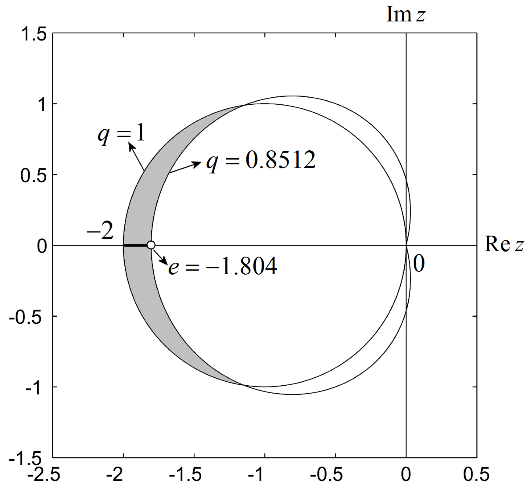
The position of Eigenvalues $e_{x,y}$, related to the stability region S for the range $q\in (0.8152,1)$, is indicated by the tick line in Figure 2.

5. Bifurcation Diagrams

To obtain a visual summary of the dynamics of the DLMFO one considers the Bifurcation Diagram (BD) with respect to the fractional order $q\in (0,1)$. As one can see in this section this useful tool should be considered for FO discrete systems with precaution not only due to the mentioned nonexistence of periodic solutions in continuous and also discrete FO systems, but also due to a non-invariance-like with respect to initial conditions (see also [41]). Thus, it is shown empirically that to every considered initial condition corresponds a different diagram which, for avoid the confusion with the BD, will be called the Bifurcative Set (BS). So, while for IO discrete systems, such as the logistic map, the BD has a unique shape for whatever initial conditions, in the sense that the diagram obtained for parameter variation has the same shape for whatever initial conditions (see also [42]), the DLMFO has the BD as “composed” of several different BSs, one for each considered initial condition. This characteristic are more evident q values close to 0.

Diagrams in this paper are obtained by integrating the system with five different initial conditions for $n_{max}=2000$ iterations, from which the first 1700 being discarded to avoid transients.

Note that for different values of q, every considered initial condition in the numerical experiment of the BD, has been iterated before drawing the diagram for $n_{max}=$ 10,000, in order to verify that the results obtained with $n_{max}=2000$ are similar to those with $n_{max}=$ 10,000 iterations, and are not prejudiced by transients. Therefore, the choice of 2000 iterations proved to be an acceptable compromise between computer time and rightness of the results.

For the sake of simplicity, one consider the diagrams for only the variable x (Figure 3). For figure clarity, only five empirically chosen initial conditions are considered: ${[x_0,y_0]}_1=[-0.5,-0.1]$ (magenta), ${[x_0,y_0]}_2=[0.2,0.1]$ (red), ${[x_0,y_0]}_3=[0.01,0.01]$ (blue), ${[x_0,y_0]}_4=[-0.5,0.3]$ (green), ${[x_0,y_0]}_5=[0.1,-0.7]$ (black). Supplementary initial conditions have been tested but the diagrams become too loaded. As can be seen, each initial condition generates a different BS.

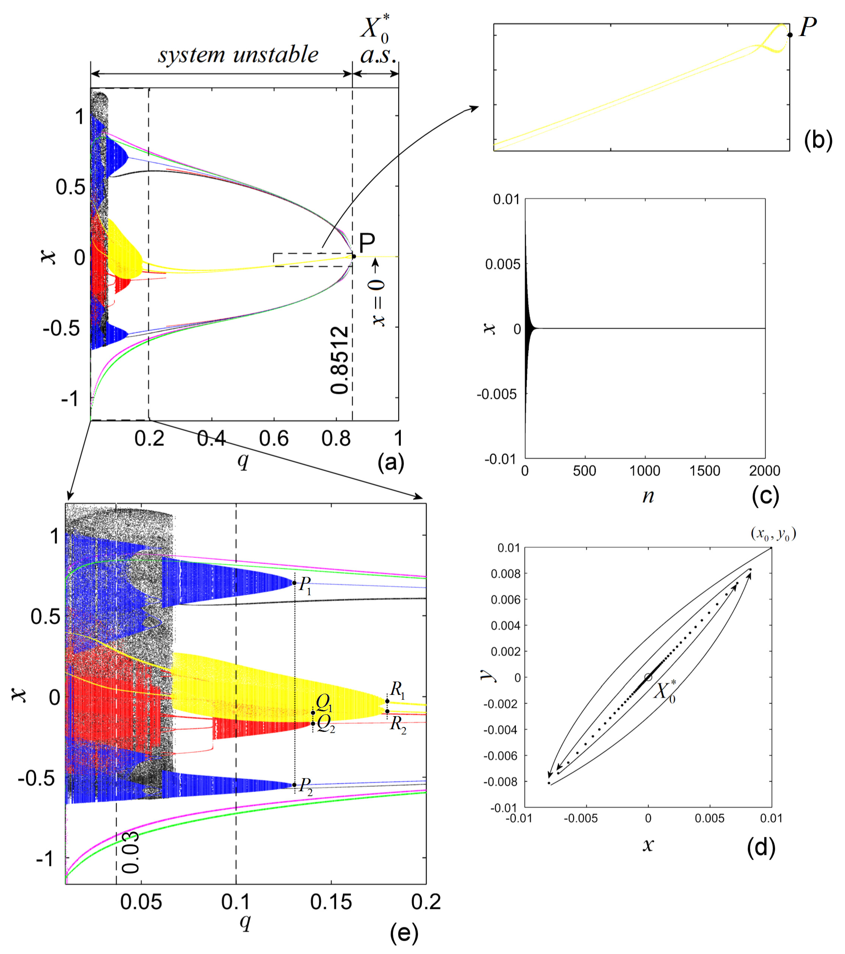
Figure 3b reveals the consistency of the analytical result of the asymptotical stability of $X_0^{*}$ with the numerical results (point P with $q=0.8512\approx {log}_{2}1.804$). Moreover, the zoom in Figure 3b shows a periodic-like orbit, which exists for $q<0.8512$. Figure 3c,d present the time series and phase plot, respectively, indicating the behavior of an orbit starting close from $X_0^{*}$, which tends asymptotically to $X_0^{*}$ for $q>0.8512$.

The following natural questions arise:

$Q_1$:

Should the BD be considered as the “reunion” of all BSs?

$Q_2$:

Considering the intensive numerical experiments which indicate that different initial conditions generates different BSs, how many such BSs can be finally obtained and which one of these BSs should be considered the “right” BD?

Hereafter, in order to avoid the problem raised by $Q_1$, by BD of the GLMFO one understands the set of all obtained BSs.

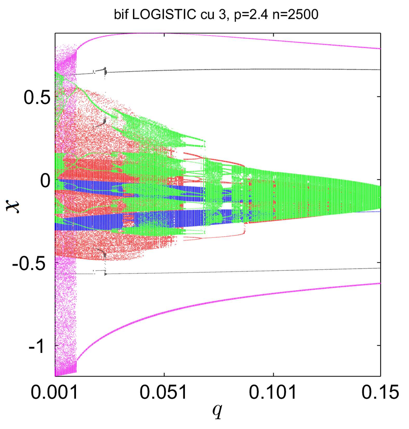
Another BD with five initial conditions $[-0.5,0.1]$ (magenta), $[0.2,0.1]$ (red), $[-0.01,0.1]$ (blue), $[0.4,0.1]$ (green) and $[0.1,0.1]$ (black), presented in Figure 4, underlines the differences between BSs, even for $y_0$ kept constant ($y_0=0.1$).

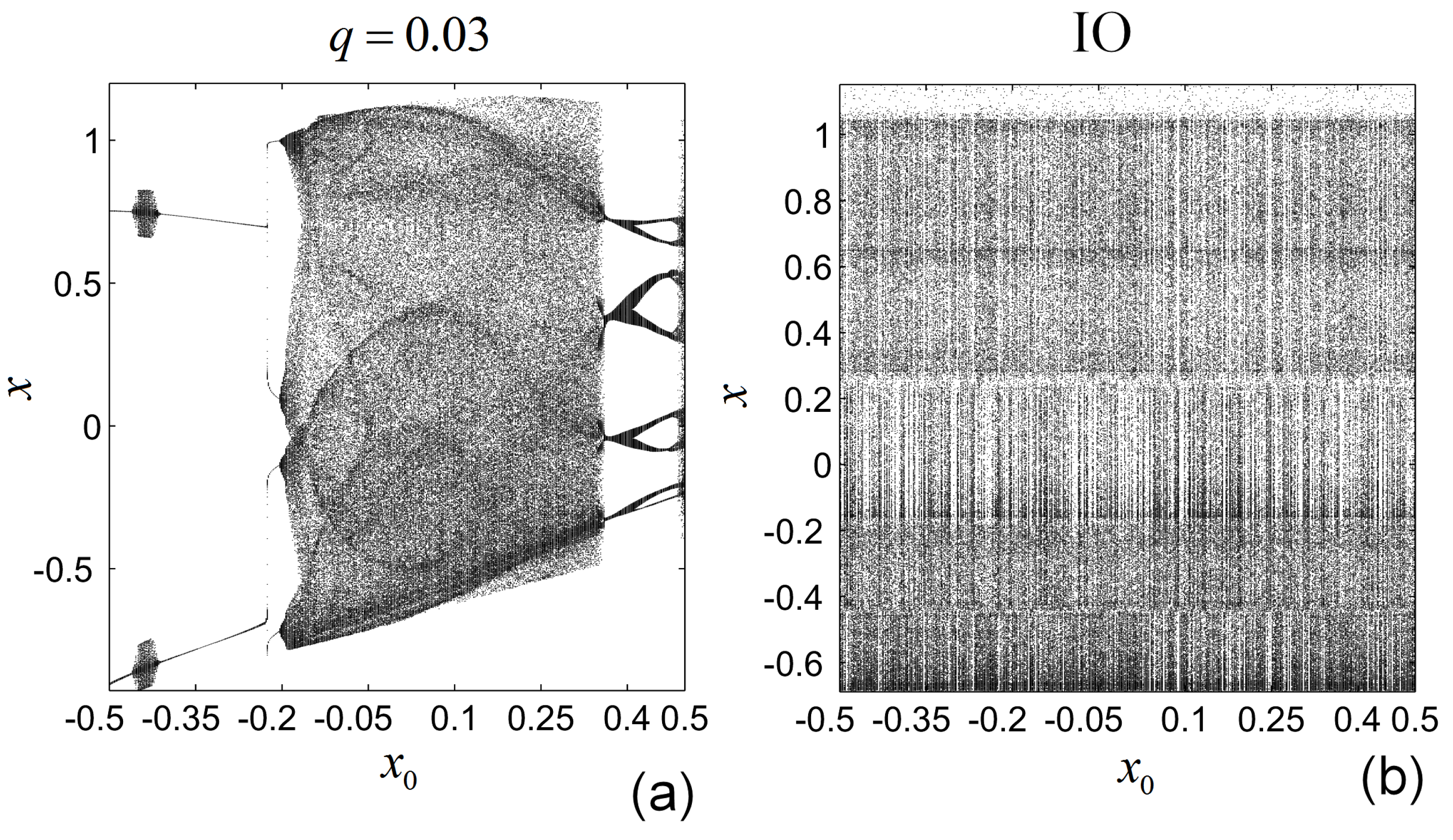
The following experiment reveals the fact that for any of 600 considered initial conditions $[x_0,y_0]$ within the segment $[x_0,0.8]$, for $x_0\in [0.5,0.5]$, and $q=0.03$, in the bifurcation diagram vs. initial condition, $x_0$ and with $y_0$ constant, there correspond different attractors (Figure 5a). Because there are an infinity of points within the considered segment, one can extrapolate the idea that to every initial condition there exist different BSs. On the other side, from Figure 5b one can see that for the IO case of the considered system, the initial conditions $x_0$ give birth to similar (chaotic) attractors. This is in agreement with the cases of IO other discrete and continuous systems where BDs do not present such sensible dependence on initial conditions.

To better understand the differences between the IO cases and FO cases, consider the sketch in Figure 6, where two BDs are considered. Figure 6a presents a BD of a discrete system of IO depending on a real parameter r (such as the logistic map), for a single value of r, while Figure 6b presents the BS of a discrete system of fractional order q (like the GLMFO) for a particular value of q. Both systems are considered as depending on the variable u. The vertical bars or points corresponding to r or q are attractors (Poincaré-like sections of BDs through r or q), attractive points or stable cycles (like), quasiperiodic (like) or chaotic attractors. As known, in both cases the chaotic behavior is characterized by the sensitive dependence of initial conditions (as first formulated by Guckenheimer [43]). However, as this paper shows, in FO systems, like the considered GLMFO, for a considered value of q all different initial conditions (in this sketch $u_{0i}$, $i=1,2\dots ,5$), could generate different regular-like, and chaotic attractors (red, yellow, blue, green, black tick lines), while in the IO case all initial conditions lead finally to a single attractor (chaotic in this sketch, black tick line), or two attractors (in the case of multistability).

Therefore, the sensitive dependence of the BD on initial conditions has different meaning from the classical notion of dependence on initial conditions (see [3]). Every BD of a FO system, considered as a set of all Poincaré sections through the axis q, which are all different, depends sensibly on the considered initial conditions, while every orbit depends sensibly on the initial condition.

Remark 2.

(i) 

Beside the dependence on initial conditions, because fractional derivatives are nonlocal operators, they present the so called memory effect which means that the actual behavior is not only influenced by the actual state of the underlying system but also by the events happened in the past. Therefore, beside the dependence on the initial conditions, at every moment n, the solutions $x_n$ and $y_n$ depends not only on $x_0$ and $y_0$ but also on all previous values $x_k$ and $y_k$, for $k=1,2,\dots ,n-1$.

(ii) 

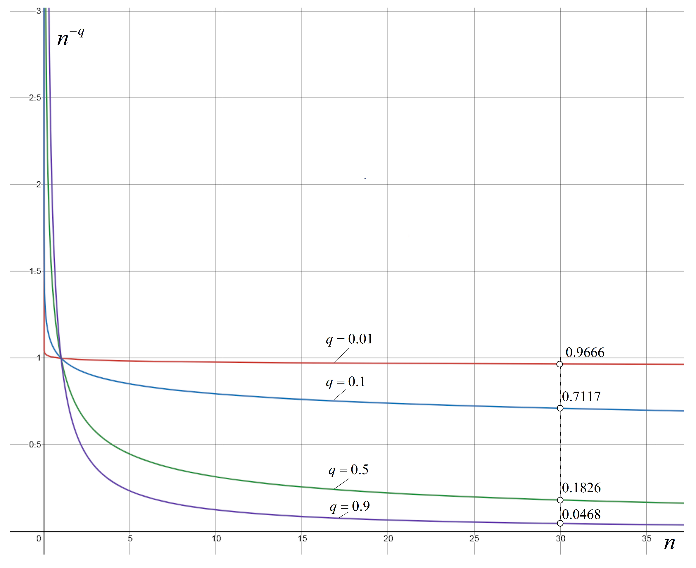
Because the decay rate of the solutions in the asymptotically stable case is $n^{-q}$ [40] (see also [14]), smaller values of q implies bigger errors, while to bigger values of q, close to 1, errors are smaller. In Figure 7, the graph of $n^{-q}$ is represented as function of n for different values of q. For clarity, only first few dozens of values n have been considered. The circles at $n=30$ indicates the order of errors for each considered values of q. If one considers $n_{max}=$ 10,000, from the curve $q=0.01$ one obtains 10,000${}^{-0.01}=0.9120$, while the curve $q=0.9$, gives 10,000${}^{-0.9}=2.5119e-004$.

Consider $q=0.1$ and the underlying attractors presented in Figure 8 (see also the dotted line in Figure 3b).

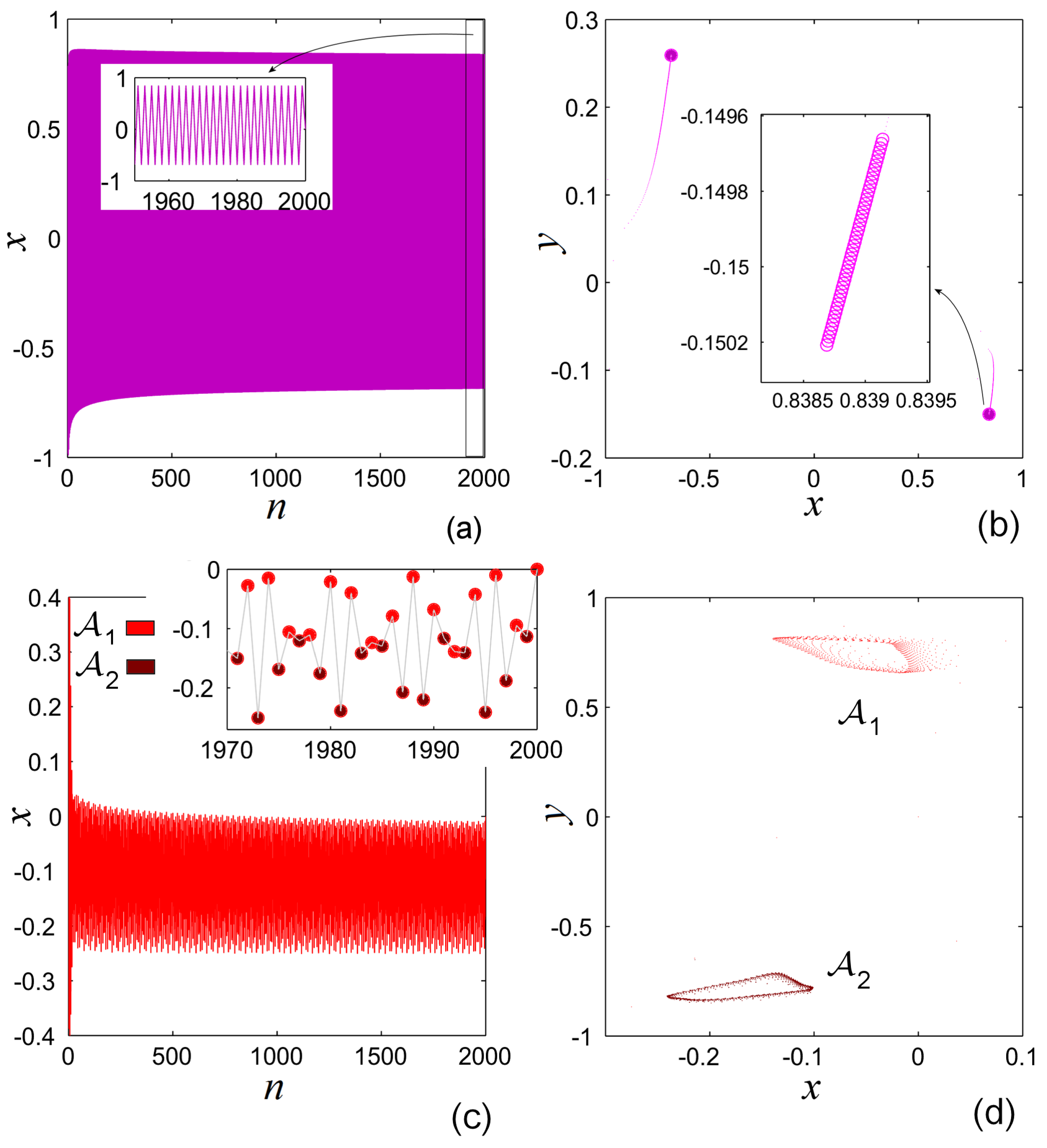
For the initial condition ${[x_0,y_0]}_1$ one obtains a periodic-like orbit (Figure 8a), a fact underlined by the zoom in phase plane representation (Figure 8b), which shows the fact that it is not about a true periodic orbit.

For ${[x_0,y_0]}_2$ one obtains a two-band quasiperiodic-like orbit (Figure 8c). The two colored filled disks indicate the alternative visiting order of the subsets denoted ${\mathcal{A}}_1$ and ${\mathcal{A}}_2$ of the quasiperiodic-like attractor (Figure 8d). To note that for $q=0.1$ similar quasiperiodicity-like orbits can be obtained with initial condition within the blue and yellow BSs.

As Figure 3e shows, there are several bifurcation-like points, the “end” points of quasiperiodic-like behavior of yellow, blue and red BSs (such as the points $P_{1,2},Q_{1,2}$ and $R_{1,2}$ or the point P in Figure 3b), related to BSs, these points have different positions in the fractional-order space (each of them take place at different values of q). Note that, by comparing with the IO case where these points would indicate Hopf bifurcations, in FO systems this is a delicate problem, since periodicity still does not exists.

6. Hidden Attractors

While generally in the cases of IO systems the attractors coexist, one of the ingredients of hidden attractors is indicated by the presence of different BSs, which seem to coexist and complement each other in a kind of harmony. In the considered case of the DLMFO (and also in some other FO discrete systems, see [3,31]) the BSs seem to be independent, having nothing to do with each other.

Let us find the potential hidden chaotic attractors for q within the range $(0,0.06)$, where the BSs indicates chaotic behavior. As for this range of q the fixed points are unstable, one can consider that the corresponding chaotic attractors are hidden (see the characterization of hidden attractors in Introduction).

As the BSs show (Figure 3a), there exists periodic chaos, when in the BD, the chaotic attractor consists of several vertical bands and even a typical orbit fills out every of the interval irregularly, the successive iterations visit them periodically.

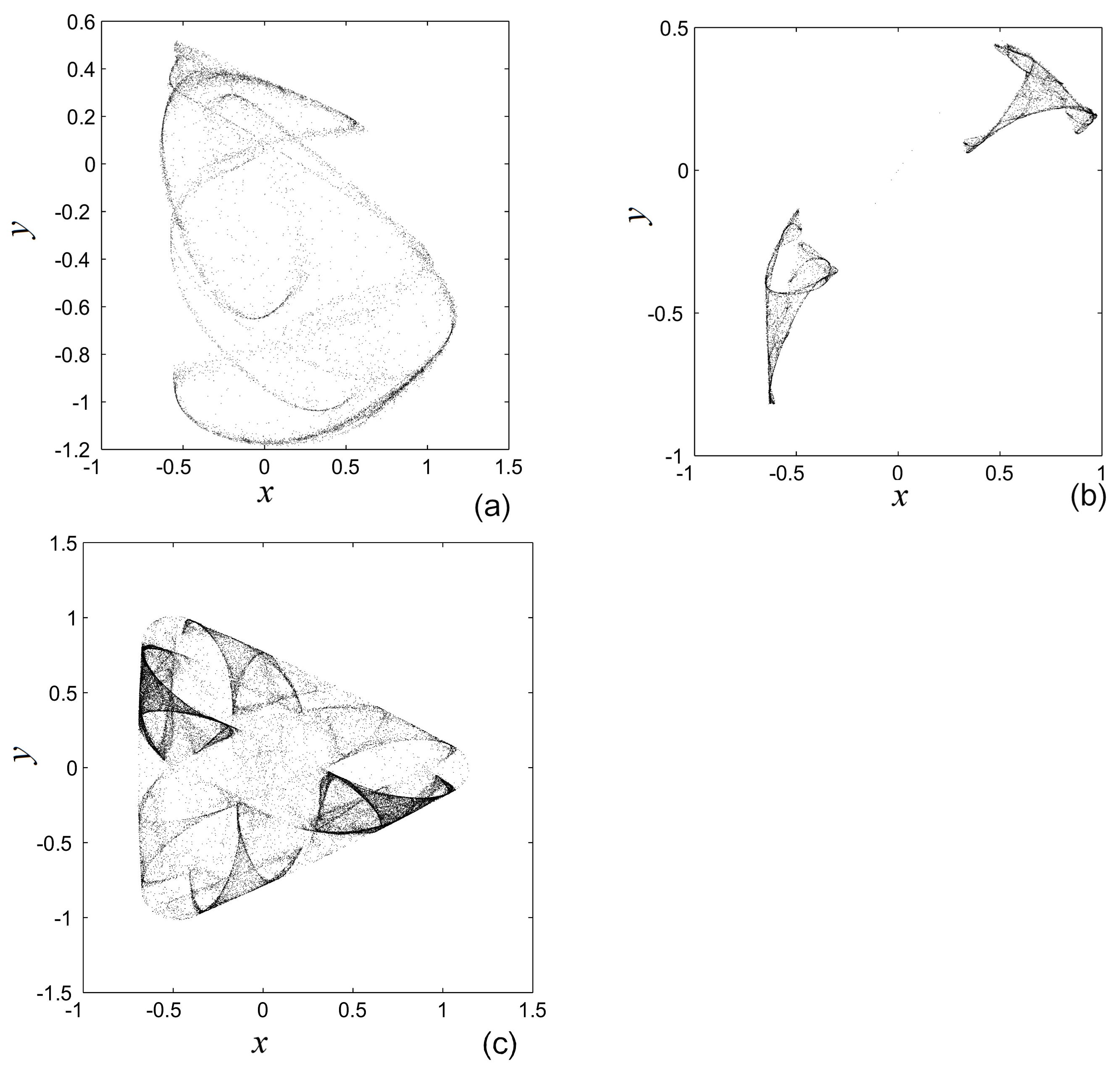
For example, for $q=0.03$ and the initial condition ${[x_0,y_0]}_5$, one obtains the hidden chaotic attractor presented in Figure 9a. The projection on the $Ox$ axis reveals a connected set, as shown by the one-band chaotic segment in the cross-section of the black BS with the line $q=0.03$. Another hidden chaotic attractor identified in the blue BS, for the initial condition ${[x_0,y_0]}_3$, which is composed by two disconnected sets (two-band chaotic segments in the cross section of the blue BS with the line $q=0.03$) is presented in Figure 9b). If one approaches the zero value of q such as $q=0.005$, for $[x_0,y_0]=[-0.01,-0.01]$ one obtains another chaotic attractor (Figure 9c) which resembles with the IO counterpart (Figure 1).

The numerical experiments show that for $q\in (0,0.06)$, all BSs give birth hidden chaotic (for $q\in (0,0.06)$), or periodic-like (for $q\in (0,1)$), attractors.

As mentioned in $Q_2$ it is difficult to specify the real number of these hidden attractors.

7. Symmetry Broken by the Fractional Order

Another interesting property of this system, which probably is due to the fractionality is the fact that, compared with its counterpart IO map, the considered chaotic attractors in Figure 9a–c, present a dihedral $D_3$ symmetry-broken.

Consider first the DLM of IO with the typical chaotic attractor depicted in Figure 1 and the reflection (mirror) lines through the center (origin), $\left(a\right),\left(b\right),\left(c\right)$. As can be seen, due to the slow convergence, almost every point can be considered as the mirror of some other point with respect one of the axes, or obtained with a rotation.

For example, consider the clear visible point A in Figure 1 with coordinates $x_A=0.3216$, $y_A=0$ and rotate it counterclockwise around the origin O with ${120}^{\circ }$ (red arrow), i.e., $R_1$ (1).

The new point B will have the coordinates

$$\left(\begin{array}{c}{x}_B\\ y_B\end{array}\right)=R_1·A=\frac{1}{2}\left(\begin{array}{cc}-1& -\sqrt{3}\\ \sqrt{3}& -1\end{array}\right)\left(\begin{array}{c}0.3216\\ 0\end{array}\right)=\left(\begin{array}{c}-0.1606\\ 0.2781\end{array}\right),$$

with a good approximation of the graphically determined coordinates.

The same point B can be also obtained with the symmetry $S_1$ (2) across the line $\left(b\right)$ (red dotted line) which makes an angle $\pi /3$ with the horizontal axis

$$\left(\begin{array}{c}{x}_B\\ y_B\end{array}\right)=S_1·A=\frac{1}{2}\left(\begin{array}{cc}-1& \sqrt{3}\\ \sqrt{3}& 1\end{array}\right)\left(\begin{array}{c}0.3216\\ 0\end{array}\right)=\left(\begin{array}{c}-0.1606\\ 0.2781\end{array}\right).$$

Actually one can consider that all points of the IO attractor are generated by rotations or symmetries.

The next result regards the symmetries of the DLMFO.

Theorem 3.

Attractors of the DLMFO have not $D_3$ symmetries.

Proof. 

Consider first the IO and the symmetry with respect the horizontal axis (symmetry axis $\left(a\right)$), i.e., $S_0$. Applied to some point $(x,y)$ one has

$$S_0(x,y)=S_0\left(\begin{array}{c}x\\ y\end{array}\right)=\left(\begin{array}{cc}1& 0\\ 0& -1\end{array}\right)\left(\begin{array}{c}x\\ y\end{array}\right)=\left(\begin{array}{c}x\\ -y\end{array}\right)=(x,-y),$$

(15)

and due to the parity of functions $f_{1,2}(x,y)$ in (5) ($f_1$ and $f_2$ are even and odd, respectively), from (3) one obtains:

$$\begin{array}{cc}\hfill & f\left(S_0(x,y)\right){=f(x,y)|}_{(x,y)=(x,-y)}=\hfill \\ & \left(\begin{array}{c}-1.8040x_{n-1}+x_{n-1}^3+x_{n-1}{y}_{n-1}^2+0.5x_{n-1}^2-0.5y_{n-1}^2\\ -1.8040(-y_{n-1})+(-y_{n-1})x_{n-1}^2+{(-y_{n-1})}^3-x_{n-1}(-y_{n-1})\end{array}\right)=\left(\begin{array}{c}{f}_1(x,y)\\ -f_2(x,y)\end{array}\right)\hfill \end{array}$$

On the other side:

$$S_0\left(f(x,y)\right)=S_{0}f(x,y)=\left(\begin{array}{cc}1& 0\\ 0& -1\end{array}\right)\left(\begin{array}{c}{f}_1(x,y)\\ f_2(x,y)\end{array}\right)=\left(\begin{array}{c}{f}_1(x,y)\\ -f_2(x,y)\end{array}\right).$$

Therefore, $f\left(S_0(x,y)\right)=S_0\left(f(x,y)\right)$. The second condition (3) can be proved similarly.

Consider next the FO case and denote the map of the right hand side of (12) as

$$F(x,y)=\left(\begin{array}{c}{x}_0+F_1(x,y)\\ y_0+F_2(x,y)\end{array}\right),$$

(16)

where

$$F_1(x,y)={\displaystyle \frac{1}{\mathsf{\Gamma }\left(q\right)}\sum _{i=1}^n\frac{\mathsf{\Gamma }(n-i+q)}{\mathsf{\Gamma }(n-i+1)}(-1.804x_{i-1}+x_{i-1}^3+x_{i-1}{y}_{i-1}^2+0.5x_{i-1}^2-0.5y_{i-1}^2)},$$

and

$$F_2(x,y)={\displaystyle \frac{1}{\mathsf{\Gamma }\left(q\right)}\sum _{i=1}^n\frac{\mathsf{\Gamma }(n-i+q)}{\mathsf{\Gamma }(n-i+1)}(-1.804y_{i-1}+y_{i-1}{x}_{i-1}^2+y_{i-1}^3-x_{i-1}{y}_{i-1})},$$

where, for the sake of simplicity, the parameter n and index i in $F_{1,2}$ are omitted.

Following the way used to verify the symmetry for the IO case, by using the parity properties of $F(x,y)$ defined in (16) and following (15) one obtains:

$$F\left(S_0(x,y)\right){=F(x,y)|}_{(x,y)=(x,-y)}=\left(\begin{array}{c}{x}_0+F_1(x,y)\\ y_0-F_2(x,y)\end{array}\right).$$

(17)

On the other side:

$$S_0\left(F(x,y)\right)=\left(\begin{array}{cc}1& 0\\ 0& -1\end{array}\right)\left(\begin{array}{c}{x}_0+F_1(x,y)\\ y_0+F_2(x,y)\end{array}\right)=\left(\begin{array}{c}{x}_0+F_1(x,y)\\ -y_0-F_2(x,y)\end{array}\right),$$

(18)

and, therefore, $F\left(S_0(x,y)\right)\ne S_0\left(F(x,y)\right)$. □

Actually, the explanation of this result lies in the mentioned time history of numerical methods for continuous and also discrete systems of FO. This symmetry broken is also presumably due to the influence of the fractional order q and seems to be more powerful as the q increases. As can be seen from (17) and (18), if $y_0=0$, the influence of $y_0$ disappears and symmetry should maintains. However, for $y_0=0$, $y_n=0$ for all n and the attractors starting from $[x_0,0]$ collapse on the axis $Ox$, case which is not considered here. Thus, while for the hidden chaotic attractors in Figure 7a,b obtained for $q=0.03$ the symmetry destroyed, the attractor in Figure 7c with $q=0.01$ resembles with the its IO counterpart in Figure 1, but is still non-symmetric.

8. Discussion

In this paper, one of Golubitsky’s maps of IO (dihedral logistic map) has been considered in the FO discrete form. The IO variant presents dihedral $D_3$ symmetry which is lost in the FO variant. It is shown that only few hundreds iteration are not enough to discard transients and to obtain accurate results. As in some previous studied discrete systems of FO [3], the bifurcation diagram seems to be composed by several different sets, called bifurcative sets, one for each initial condition, which indicate attractors coexistence. In other words, the bifurcative sets depend sensibly on initial conditions, but in a different sense for the classical meaning of the sensitive dependence on initial conditions of an orbit. Probably due to the convergence of the integration method, for smaller values of q (close to 0), the differences between the bifurcative sets are significant, while for q tending to 1, these sets seem to tend one to each other. The instability of the system (due to the instability of fixed points) and the existence of several bifurcative sets could be considered ingredient to find hidden attractors. However, finding their exact number is a difficult if not an impossible task due to the dependence of the bifurcative sets on the initial conditions. Additionally, the numerical approach of this system (and probably of other discrete systems of FO) indicates that the tools like bifurcation diagram, or hidden attractors require much more attention.

References

- Oldham, K.; Spanier, J. The Fractional Calculus: Theory and Applications of Differentiation and Integration to Arbitrary Order; Academic Press: New York, NY, USA, 1974. [Google Scholar]
- Podlubny, I. Geometric and physical interpretation of fractional integration and fractional differentiation. Fract. Calc. Appl. Anal. 2002, 5, 367–386. [Google Scholar]
- Danca, M.-F.; Feckan, M.; Kuznetsov, N.; Chen, G. Coupled Discrete Fractional-Order Logistic Maps. Mathematics 2021, 9, 2204. [Google Scholar] [CrossRef]
- Area, I.; Losada, J.; Nieto, J. On Fractional Derivatives and Primitives of Periodic Functions. Abstr. Appl. Anal. 2014, 2014, 392598. [Google Scholar] [CrossRef] [Green Version]
- Fečkan, M. Note on Periodic and Asymptotically Periodic Solutions of Fractional Differential Equations. In Studies in Systems, Decision and Control; Springer: Cham, Switzerland, 2020; Volume 177, pp. 153–185. [Google Scholar]
- Kang, Y.M.; Xie, Y.; Lu, J.; Jiang, J. On the nonexistence of non-constant exact periodic solutions in a class of the Caputo fractional-order dynamical systems. Nonlinear Dyn. 2015, 82, 1259–1267. [Google Scholar] [CrossRef]
- Kaslik, E.; Sivasundaram, S. Non-existence of periodic solutions in fractional-order dynamical systems and a remarkable difference between integer and fractional-order derivatives of periodic functions. Nonlinear Anal. Real World Appl. 2012, 13, 1489–1497. [Google Scholar] [CrossRef] [Green Version]
- Shen, J.; Lam, J. Non-existence of finite-time stable equilibria in fractional-order nonlinear systems. Automatica 2014, 50, 547–551. [Google Scholar] [CrossRef]
- Tavazoei, M.; Haeri, M. A proof for non existence of periodic solutions in time invariant fractional order systems. Automatica 2009, 45, 1886–1890. [Google Scholar] [CrossRef]
- Tavazoei, M. A note on fractional-order derivatives of periodic functions. Automatica 2010, 46, 945–948. [Google Scholar] [CrossRef]
- Yazdani, M.; Salarieh, H. On the existence of periodic solutions in time-invariant fractional order systems. Automatica 2011, 47, 1834–1837. [Google Scholar] [CrossRef]
- Bin, H.; Huang, L.; Zhang, G. Convergence and periodicity of solutions for a class of difference systems. Adv. Differ. Equ. 2006, 2006, 70461. [Google Scholar] [CrossRef] [Green Version]
- Diblík, J.; Fečkan, M.; Pospisil, M. Nonexistence of periodic solutions and S-asymptotically periodic solutions in fractional difference equations. Appl. Math. Comput. 2015, 257, 230–240. [Google Scholar] [CrossRef]
- Edelman, M. Caputo standard α-family of maps: Fractional difference vs. fractional. Chaos 2014, 24, 023137. [Google Scholar] [CrossRef] [Green Version]
- Edelman, M. On stability of fixed points and chaos in fractional systems. Chaos 2018, 28, 023112. [Google Scholar] [CrossRef]
- Jonnalagadda, J. Periodic Solutions Of Fractional Nabla Difference Equations. Commun. Appl. Anal. 2016, 20, 585–610. [Google Scholar]
- Pospíšil, M. Note on fractional difference equations with periodic and S-asymptotically periodic right-hand side. Nonlinear Oscil. 2021, 24, 99–109. [Google Scholar]
- Jafari, S.; Sprott, J.; Nazarimehr, F. Recent new examples of hidden attractors. Eur. Phys. J. Spec. Top. 2015, 224, 1469–1476. [Google Scholar] [CrossRef]
- Kuznetsov, N. Theory of hidden oscillations and stability of control systems. J. Comput. Sys. Sc. Int. 2020, 59, 647–668. [Google Scholar] [CrossRef]
- Leonov, G.; Kuznetsov, N. Hidden attractors in dynamical systems. From hidden oscillations in Hilbert-Kolmogorov, Aizerman, and Kalman problems to hidden chaotic attractors in Chua circuits. Int. J. Bifurc. Chaos Appl. Sci. Eng. 2013, 23, 1330002. [Google Scholar] [CrossRef] [Green Version]
- Leonov, G.; Kuznetsov, N.; Mokaev, T. Homoclinic orbits, and self-excited and hidden attractors in a Lorenz-like system describing convective fluid motion. Eur. Phys. J. Spec. Top. 2015, 224, 1421–1458. [Google Scholar] [CrossRef] [Green Version]
- Anastassiou, G.A. Discrete fractional calculus and inequalities. arXiv 2009, arXiv:0911.3370. [Google Scholar]
- Bastos, N.R.O.; Ferreira, R.A.C.; Torres, D.F.M. Discrete-time fractional variational problems. Signal Process. 2011, 91, 513–524. [Google Scholar] [CrossRef] [Green Version]
- Cheng, J.-F.; Chu, Y.-M. On the fractional difference equations of order (2,q). Abstr. Appl. Anal. 2011, 2011, 497259. [Google Scholar] [CrossRef] [Green Version]
- Atici, F.M.; Eloe, P.W. Discrete fractional calculus with the nabla operator. Electron. J. Qual. Theory Differ. Equ. 2009, 3, 1–12. [Google Scholar] [CrossRef]
- Cheng, J.-F.; Chu, Y.-M. Fractional Difference Equations with Real Variable. In Abstract and Applied Analysis, Advanced Theoretical and Applied Studies of Fractional Differential Equations; Hindawi: London, UK, 2012; p. 918529. [Google Scholar]
- Jarad, F.; Abdeljawad, T.; Baleanu, D.; Biçen, K. On the stability of some discrete fractional nonautonomous systems. Abstr. Appl. Anal. 2012, 2012, 476581. [Google Scholar] [CrossRef]
- Rajagopal, K.; Panahi, S.; Chen, M.; Jafari, S.; Bao, B. Suppressing spiral wave turbulence in a simple fractional-order discrete neuron map using impulse triggering. Fractals 2021, 29, 2140030. [Google Scholar] [CrossRef]
- Danca, M.F.; Kuznetsov, N. Hidden chaotic sets in a Hopfield neural system. Chaos Solitons Fractals 2017, 103, 144–150. [Google Scholar] [CrossRef]
- Danca, M.-F.; Feckan, M.; Kuznetsov, N. Chaos control in the fractional order logistic map via impulses. Nonlinear Dyn. 2019, 98, 1219–1230. [Google Scholar] [CrossRef] [Green Version]
- Danca, M.F. Puu System of Fractional Order and Its Chaos Suppression. Symmetry 2020, 12, 340. [Google Scholar] [CrossRef] [Green Version]
- Field, M.; Golubitsky, M. Symmetric Chaos: How and Why. N. Am. Math. Soc. 1995, 42, 241–244. [Google Scholar]
- Field, M.; Golubitsky, M. Symmetry in Chaos; A Search for Pattern in Mathematics, Art and Nature, 2nd ed.; Society for Industrial and Applied Mathematics: Philadelphia, PA, USA, 2009. [Google Scholar]
- Chossat, P.; Golubitsky, M. Symmetry-increasing bifurcation of chaotic attractors. Physica D 1988, 32, 423–436. [Google Scholar] [CrossRef]
- Romera, M. Técnica de los sistemas dinámicos discretos (Textos Universitarios) (Spanish Edition) Paperback Consejo Superior de Investigaciones Cientificás; Consejo Superior de Investigaciones Cientificas: Serrano, Spain, 1997. [Google Scholar]
- Chen, F.; Luo, X.; Zhou, Y. Existence results for nonlinear fractional difference equation. Adv. Differ. Equ. 2011, 2011, 713201. [Google Scholar] [CrossRef] [Green Version]
- Abdeljawad, T. On Riemann and Caputo fractional differences. Comput. Math. Appl. 2011, 62, 1602–1611. [Google Scholar] [CrossRef] [Green Version]
- Atici, F.M.; Eloe, P.W. Initial value problems in discrete fractional calculus. Proc. Am. Math. Soc. 2007, 137, 981–989. [Google Scholar] [CrossRef]
- Stuart, A.; Humphries, A.R. Dynamical Systems and Numerical Analysis; Part of Cambridge Monographs on Applied and Computational Mathematics; Cambridge University Press: Cambridge, UK, 1999. [Google Scholar]
- Čermak, J.; Gyǒri, I.; Nechvátal, L. On explicit stability conditions for a linear fractional difference system. Fract. Calc. Appl. Anal. 2015, 18, 651–672. [Google Scholar] [CrossRef]
- Wang, Y.; Liu, S.; Li, H. On fractional difference logistic maps: Dynamic analysis and synchronous control. Nonlinear Dyn. 2020, 102, 579–588. [Google Scholar] [CrossRef]
- Prousalis, A.D.; Volos, C.K.; Bocheng, B.; Meletlidou, E.; Stouboulos, I.N.; Kyprianidis, I.M. Chapter 6—Extreme Multistability in a Hyperjerk Memristive System with Hidden Attractors. In Emerging Methodologies and Applications in Modelling, Recent Advances in Chaotic Systems and Synchronization; Boubaker, O., Jafari, S., Eds.; Academic Press: Cambridge, MA, USA, 2019; pp. 89–103. [Google Scholar]
- Guckenheimer, J. Sensitive dependence on initial conditions for one-dimensional maps. Commm. Math. Phys. 1979, 70, 133–160. [Google Scholar] [CrossRef]
Figure 1.
A -symmetric image of the DLM of IO (7). In red is indicated the counterclockwise rotation with applied to the point A to obtain the point B which is symmetric with respect the line (b).
Figure 2.
Stability domain S in the case of the fixed point . Tick line represents the asymptotic stability range of q for .
Figure 3.
DLM of FO. (a) Bifurcation diagram vs. q. The bifurcation-like point P indicates the beginning of the stability of for ; (b) zoomed image; (c) time series tending to the asymptotically stable fixed point for ; (d) phase portrait with the orbit points indicating the evolution of the orbit to ; (e) zoomed area of the bifurcation diagram.
Figure 4.
Another bifurcation diagram vs. for initial conditions , , , , .
Figure 5.
Bifurcation diagrams of the DLM of FO and IO versus the initial conditions and . (a) The FO case ; (b) the IO case.
Figure 6.
Sketch of diagrams of bifurcations. (a) The IO case; (b) FO case. , are initial conditions.
Figure 7.
Graph of for different values of q.
Figure 8.
Two orbits of the DLM of FO for . (a) Time series of a periodic-like orbit from ; (b) phase portrait of the orbit and a zoom indicating the slow orbit convergence; (c) time series of a two-band quasiperiodic-like orbit from . The zoom indicates the alternate pattern of the orbit between the two subsets and (red and brown) of the quasiperiodic-like attractor; (d) phase portrait of the orbit .
Figure 9.
Hidden chaotic attractors of the DLMFO with broken-symmetry. (a) and . (b) and ; (c) , and .
Publisher’s Note: MDPI stays neutral with regard to jurisdictional claims in published maps and institutional affiliations. |
© 2022 by the authors. Licensee MDPI, Basel, Switzerland. This article is an open access article distributed under the terms and conditions of the Creative Commons Attribution (CC BY) license (https://creativecommons.org/licenses/by/4.0/).
Share and Cite
MDPI and ACS Style
Danca, M.-F.; Kuznetsov, N. D3 Dihedral Logistic Map of Fractional Order. Mathematics 2022, 10, 213. https://doi.org/10.3390/math10020213
AMA Style
Danca M-F, Kuznetsov N. D3 Dihedral Logistic Map of Fractional Order. Mathematics. 2022; 10(2):213. https://doi.org/10.3390/math10020213
Chicago/Turabian StyleDanca, Marius-F., and Nikolay Kuznetsov. 2022. "D3 Dihedral Logistic Map of Fractional Order" Mathematics 10, no. 2: 213. https://doi.org/10.3390/math10020213
Note that from the first issue of 2016, this journal uses article numbers instead of page numbers. See further details here.