
Chaotic Oscillations in Cascoded and Darlington-Type Amplifier Having Generalized Transistors


Department of Radio Electronics, Brno University of Technology, Technicka 12, 616 00 Brno, Czech Republic
*
Author to whom correspondence should be addressed.
Mathematics 2022, 10(3), 532; https://doi.org/10.3390/math10030532
Submission received: 11 January 2022
/
Revised: 4 February 2022
/
Accepted: 6 February 2022
/
Published: 8 February 2022
(This article belongs to the Special Issue Chaotic Systems: From Mathematics to Real-World Applications)
Abstract
:This paper describes, based on both numerical and experimental bases, the evolution of chaotic and, in some cases, hyperchaotic attractors within mathematical models of two two-port analog functional blocks commonly used inside radio-frequency systems. The first investigated electronic circuit is known as the cascoded class C amplifier and the second network represents a resonant amplifier with Darlington’s active part. For the analysis of each mentioned block, fundamental configurations that contain coupled generalized bipolar transistors are considered; without driving force or interactions with other lumped circuits. The existence of the structurally stable strange attractors is proved via the high-resolution composition plots of the Lyapunov exponents, numerical sensitivity analysis and captured oscilloscope screenshots.
1. Introduction
A unique nonlinear phenomenon currently denoted as chaos and hyper chaos has been intensively studied in the lumped electronic circuits for nearly four decades. The motivation of such research is to explain the complex movement of dynamical systems, where extreme sensitivity of system solutions to tiny changes and/or uncertainties of the initial conditions cooperates with some folding mechanism. Therefore, the vector field needs to be arranged such that there are subspaces where nearby trajectories are separated and regions where these are folded back, resulting in a bounded dense attractor. During this research, chaos turned from preliminary theories into mature knowledge with many successful contributions and problems solved. Let us shorten the extensive list of publications oriented to chaos in the analog circuits and show only a small, but very interesting, number of examples.
The oldest and, at the same time probably one of the simplest, chaotic oscillators is based on connection between the parallel LC resonant tank, timing network and nonlinear active resistor. This two-terminal element can be considered with either piecewise linear [1] or low-order polynomials, usually cubic [2,3] ampere-voltage characteristics. After the discovery of the so-called Chua’s oscillator, many papers were devoted to the analysis of this circuit. Some researchers were focused on providing a rigorous proof of the existence of the chaotic solution [4], some authors were fascinated by the rich gallery of the strange attractors that can be generated by such simple circuits [5]. Formation of the typical chaotic attractors can be explained by showing geometrical aspects of the vector field [6], analysis of eigenspaces associated with equilibrium points [7], revealing various hidden attractors and demonstrate associated methodology [8], and showing topological entropy [9]. In past years, Chua’s circuit received significant attention from the application point of view. For example, a bidirectional secure communication system is described in Reference [10]. Spread spectrum communication via chaos modulation is explained in a comprehensive study [11]. None of the other chaotic circuits attract such massive attention as Chua’s oscillator does.
The genesis of Chua’s oscillator began in the 1980s with the desire to develop a robust generator of the double-scroll chaotic attractor. Stretching of a state space volume mentioned above is achieved by the unstable fixed points while the folding mechanism is covered by suitable flow transitions between individual regions of the state space (for a piecewise linear case). However, chaos was recognized as the natural behavior of conventional analog building blocks dedicated for continuous-time signal processing. For example, chaotic dynamics within a second-order phase locked loop operating as a frequency modulated demodulator that has realistic parameters is demonstrated in study [12]. The presence of dense strange attractors in a DC-DC buck converter driven by a constant amplitude pulse width modulation signal is the topic of paper [13]. During intensive research on many reputable workplaces, it turns out that chaotic waveforms can be revealed in the global dynamics of almost all power electronic systems. For a comprehensive review focused on this topic, paper [14] can be recommended to interested readers. Robust chaos can be observed within conventional analog building blocks primarily dedicated for a generation of harmonic waveforms as well as relaxation generators. For example, chaos was reported inside the Colpitts oscillator [15], Hartley topology [16], and Wien bridge-based oscillator [17], the structure having only passive RC feedback [18], and other typical configurations of oscillators. It is somehow logical since the limit cycle is a predecessor of almost all strange attractors. Of course, the evolution of chaos is successfully investigated in a large variety of atypical electronic systems, including those having the fractional order (FO) circuit elements, mem-elements, or the combination of both [19]. Quite recently, spiral-type chaos was reported from a static multi-state memory cell; details can be found in work [20]. Driven dynamical systems could be also a subject of chaotic dynamics, as is proved for frequency filters in paper [21].
Chaos and hyper chaos can be effectively distinguished from regular, geometrically much simpler forms of dynamic motion by adopting a suitable flow quantifier. In [22] the author suggests a chaos localization method by considering numerical values of LE established from data sequences obtained during simulation and/or measurement of the Colpitts oscillator. However, the used principle is described very briefly without routine implementation details and threshold specification. The same author proposed an approach for identifying deterministic chaos using the return maps. Again, the topology of the Colpitts oscillator has been adopted, for more details, the short work [23] can be addressed. Reference [24] clearly belongs to the inspirational one, since the authors use a cut-and-try heuristic method to find many original chaotic networks containing only two bipolar transistors. Although still using a stochastic-inspired optimization routine, a much more sophisticated searching-for-chaos algorithm can be found in [25]. The authors use two-step calculation of the objective function; first step check basic requirements for chaos evolution expressed in terms of the fixed points and numerical eigenvalues; second step covers estimation of Kaplan–Yorke dimension (KYD) of the strange attractors generated for the remaining individuals in the population. As an optimization tool, the authors propose a combination of differential evolution and particle swarm optimization. The topology of the strange attractor belongs to key features for finding optimal values of parameters leading to the robust chaotic behavior, as demonstrated in paper [26]. To this end, it should be noted that dozens of other lumped analog circuits exhibit robust chaotic and hyperchaotic motion, many of them with several different sets of the internal parameters. Moreover, some of these sets can be rather close to the common operation in standard application.
This paper can be roughly considered a continuation of three recently published papers providing its significant extension and new results. In work [27], a circuit element marked as the generalized bipolar transistor (GBT) was defined as the two-port device described by a 2 × 2 admittance matrix with forward trans-conductance given by a third order polynomial function. Input admittance was considered as a free parameter while output admittance is fixed to zero. Thus, GBT is biased to work as a current source. GBT has been considered as the only active element in the negative resistance oscillator based on the lambda diode in paper [28]. Using a nature-inspired stochastic optimization technique, three different sets of internal system parameters leading to topologically different strange attractors were discovered, and the robustness of generated strange attractors was numerically analyzed. A two-stage resonant amplifier having a pair of similarly biased GBT was addressed in paper [29]. In this case, a numerical search algorithm reveals several chaotic attractors and parameter regions with associated strong hyperchaotic behavior.
This paper is organized as follows. The next section is focused on the derivation process toward the mathematical models of two conventional analog autonomous signal processing blocks: the first one represents a cascoded interconnection of bipolar transistors with the parallel resonant tank considered as a load, and the second circuit is the resonant amplifier with Darlington-type formation of bipolar transistors. Initial mathematical models are subsequently simplified by considering GBT mentioned above, together with the reduction of internal system parameters which is needed to successfully start the chaos localization routine. The third section provides a thorough numerical investigation of the analyzed dynamical system using standard tools such as high-resolution multi-dimensional plots of LE, bifurcation diagrams, sensitivity analysis, energy distribution, basins of attraction, entropy, and so forth. It is shown that the suitable coupling of two GBT can result in a very complex motion having all fingerprints typical of chaotic behavior: positive largest LE, sensitive dependance of system solution to tiny changes of initial conditions, dense strange attractors, significant entropy of generated chaotic signals and a very low degree of future time predictability. In all cases, smooth polynomial vector fields are addressed. The fourth part of this paper is focused on the transparent, easy-to-follow and reproducible design of a fully analog chaotic oscillator with off-the-shelf circuit elements and dynamics that are flow-equivalent to previously addressed mathematical models. Of course, computer-aided simulation results are supported by true experimental verification, that is, gallery of the oscilloscope screenshots is provided to prove the “long-time” structural stability of observed strange attractors. Undoubtedly, due to the chosen time constants and momentum of the human eye, the captured oscilloscope screenshots cannot be long transients or numerical artifacts. Finally, concluding remarks and future possible research topics are provided.
2. Mathematical Models
In this section, we will consider very fundamental network topologies of two different analog functional blocks that are commonly used in continuous-time radiofrequency systems. The so-called cascoded resonant amplifier is the first interesting case because the cascoding technique is used for the unilaterization of the transistor stage, that is for the elimination of the unwanted feedback. The second circuit to be investigated is the conventional Darlington formation of two bipolar transistors if loaded by the parallel resonant tank. In practice, Darlington’s topology is usually used to significantly boost the amplification factor of the composite transistor since final current transfer ratio β is a product of two contributions β1⋅β2 of the respective transistors. Both circuits will be considered as the isolated systems, that is, the driving force will be iin(t) = 0. The trans-conductance of first and second GBT can be approximated by the cubic polynomial function without offset and quadratic term (odd-symmetry distortion), that is, by the form:
where are real-valued parameters defining the saturation-type shape of a forward trans-conductance of individual GBT.
2.1. Cascoded Class C Amplifier
For starters, let us assume the principal schematic of the cascoded resonant amplifier provided in Figure 1a. The primary task of the cascoding (local feedback) transistor stage is to minimize its reverse transfer, which is commonly marked as the unilaterization of two-port. However, in further text, two GBT instead of the conventional bipolar transistors will be considered. As mentioned before, GBT can be modelled using a two-port 2 × 2 admittance matrix where both input admittance y11 and backward trans-conductance y12 are positive real constants, that is, value independent on the amplitude of the processed signal. Forward trans-conductance y21 is a scalar nonlinear function allowing the evolution of complex dynamics. The initial set of the first-order ordinary differential equations that describe the cascoded resonant amplifier (see Figure 1b) where both bipolar transistors are modelled by full admittance matrix can be expressed as
where a state vector is x = (v1, v2, v3, iL)T. Single and double lines placed above individual symbols indicate parameters associated with first and second bipolar transistors respectively. Obviously, all independent node voltages are oriented towards zero, that is, ground potential. For our autonomous situation and GBT mentioned above, this mathematical model simplifies into the dynamical system that will be addressed in this paper, namely:
Note that the parasitic base-emitter capacitances of both GBT are considered significant, working accumulation elements. For the upcoming analysis, the normalized values of all accumulation elements were chosen as unity. Equilibrium structures are all real solutions of nonlinear equation dx/dt = 0. This calculation can be carried out easily, and we obtain either single or three solutions:
depending on the signum of square root argument inside auxiliary variable:
For upcoming search-for-chaos procedure, only characteristic polynomial associated with fixed point located at origin should be evaluated symbolically,
where E represents a square unity matrix and linearization matrix is calculated near origin. A deeper analysis of polynomial (6) will reveal that a non-zero backward trans-conductance of GBT are mandatory since leads to the eigenvalues
and gives rise to stable and center manifolds associated with the equilibrium point at origin.
Obviously, dynamical system (3) can be easily modified for a non-resonant load of the cascoded amplifier. This is close to the situation where cascoded building blocks interact with a power amplifier that forms a final stage. Doing so, the number of state variables is reduced by one such that we are experiencing a third-order autonomous dynamical system of the form:
where R represents a normalized value of the load resistor. In this case, are essential for a self-excited attractor driven by the unstable fixed point located at the origin. For zero backward trans-conductance, the origin becomes a stable node characterized by the eigenvalues:
Note that the existence of the stable equilibria at origin does not prevent the analyzed dynamical system from behaving chaotically. This proposition stands for fourth order and third order systems as well. Close neighborhoods of origin need not be part of the basin of attraction for strange attractors.
2.2. Resonant Amplifier with Darlington’s Subcircuit
Assume a principal schematic of a resonant amplifier based on well-known Darlington interconnection of two GBT (Figure 2a) and equivalent autonomous AC circuit provided in Figure 2b. Straightforward analysis yields the following describing set of the first order ordinary differential equations:
Because of uniform circuit denotation, the state vector is again x = (v1, v2, v3, iL)T. Note that the parasitic base-emitter capacitances are large and contribute to the main time domain process. Now let us consider the autonomous case of this circuit and two-port admittance parameters associated with both GBT. The starting set of ordinary differential Equation (10) transforms into:
Note that all accumulation elements, including parasitic ones, are considered as working and their normalized values equal unity. In practice, this situation can be actual in high-frequency applications or if are utilized to set-up the biasing point. This dynamical system possesses one or three fixed points, that is, solutions of dx/dt = 0, namely:
where auxiliary variable
Local vector field geometry near equilibrium located at origin can be determined by the eigenvalues, that is, the roots of characteristic polynomials. Therefore, for future investigations involving system stability near zero, this fourth order polynomial should be evaluated in symbolic form:
where E and represent the unity matrix and linearization of the flow respectively. For this moment, assume that the backward trans-conductances of both GBT are zero, . In this specific case, eigenvalues associated with fixed point are
By definition, parameters are greater than zero. Therefore, origin is the non-repelling fixed point and cannot generate self-excited complex attractors.
Now, let us suppose the non-resonant amplifier with a Darlington-type cell without an input signal. It means that the resistor instead of the inductor is connected in parallel with the output capacitor. Therefore, a new system has only three degrees of freedom and is described by the following set of ordinary differential equations:
where R is a normalized value of load resistor. For this moment only, assume that backward trans-conductances of both GBT are zero, that is, . In this specific case, the eigenvalues associated with the fixed point are given by formula (15) and . Because of non-zero positive values of , the origin is the non-repelling fixed point. Therefore, the presence of backward trans-conductances of both GBT are essential for the evolution of chaos and hyperchaos excited by the unstable equilibrium point. However, it is still possible that the analyzed dynamical system exhibits multi-stability and/or generates one or several hidden strange attractors, that is, attractors not connected to the unstable fixed points.
3. Numerical Analysis
In the previous section, mathematical models of analyzed circuits are defined and treated symbolically, that is, without the knowledge of numerical values of internal parameters and initial conditions that leads to the robust chaotic and hyperchaotic oscillations. Both analog functional blocks defined above undergo the searching for chaos algorithm based on a two-step nature-inspired optimization technique. In the initial form, up to fourteen internal system parameters form hyperspace dedicated for optimization, namely the following set: . Clearly, this represents too many possible combinations for a full-grid calculation as well as for the heuristic approach. Let us find how to reduce this dimension and shrink mentioned hyperspace, preferably by introducing some physically reasonable presumptions for numerical values of circuit parameters. However, reduction needs to be chosen about maintaining the possibility of robust chaos and/or hyperchaos evolution.
Of course, all parameters are positive real values. Firstly, since accumulation elements represent the frequency scaling factors, these can be removed from investigated parameters and assumed to be unity. As will be proved later, normalized inductance L = 1 H and the equivalency of normalized capacitances still allow us to find robust chaotic behavior within this autonomous fourth order circuit. To further reduce this dimension, both GBT provides zero output admittances, that is, . At this moment, the hyperspace that undergoes the searching algorithm becomes eight dimensional. To speed-up the searching procedure, the mentioned hyperspace should be further reduced by excluding areas with an inappropriate combination of numerical values of circuit parameters. To be more specific, the sought strange attractors belong to the self-excited, excited by unstable fixed point located at the state space origin. Therefore, the unstable nature of these equilibria (with either one- or two-dimensional unstable manifold) should always be preserved. The latter case, that is the existence of the saddle-focus local geometry of vector field near origin, is tested by the calculation of roots of characteristic polynomials during each iteration step of stochastic optimization. Inappropriate configuration is fully discarded, and the dynamic behavior of the corresponding individual is not quantified. Note that the origin is the equilibrium point for all possible combinations of circuit parameters. Here is the right place to emphasize that these restrictions are not introduced with respect to the physical meaning of the analyzed circuit. The biasing of individual transistors is hypothetical and biasing circuitry is not part of the analyzed electronic system. Finally, the numerical values of the sought system parameters are encoded into the population individual up to two decimal places (without sign definition). Speaking in terms of the optimization routine, subset of the crummy individuals is attracted toward each positive value of the largest LE that occurs within the actual population. Independent numeric evaluation of LE for arbitrary system parameters leaves the place for the parallelization of population calculations. Around local maxima (LM), another population with movement restricted to the vicinity of LM is generated, with a searching procedure that follows the rules of genetics.
Of course, many alternative searching-for-chaos methods can be found in the available literature. Curious readers are recommended to perform a deep internet search. Despite the good results of our method described above, other optimization approaches, even different dynamical flow quantifiers (objective function), can lead to success.
Initial conditions do not form the edges of optimization hyperspace since these are randomly generated in the neighborhood of a state space origin. It is because only the so-called self-excited strange attractors are addressed.
Numerical analysis provided in the upcoming subsections is based on fourth order Runge–Kutta integration method with fixed step size. The normalized numerical values discovered for two GBT-based cascoded as well as Darligton-based resonant amplifier are provided. Each system is subsequently analyzed with respect to LE, KYD, energy distribution, and sensitivity.
3.1. Cascoded Class C Amplifier
The Matlab routine for chaos localization mentioned above and supplemented by a CPU-based multi-core parallel processing recognized the robust chaotic movement of cascoded resonant amplifier for following set of free parameters:
During the search algorithm, two topologically distinct strange attractors located on a plane fragment were discovered. By keeping the remaining parameters the same as those provided in group (17), the linear coefficients of the forward trans-conductance can be changed to combination , for the second type and for the last case discovered, the third type of a chaotic attractor, respectively. In general, dynamical system (3) turns into simple set of differential equations:
where symbol < introduces alternative numerical values for the second and third types of the strange state attractor. In fact, this deterministic dynamical system represents a new chaotic system with an interesting shape of strange attractor.
Figure 3 provides a numerical analysis of dynamical system (18). Three typical strange attractors were numerically integrated using Mathcad 15 and uniform initial conditions , final time 1000 s and time step 10 ms. This figure demonstrates the sensitivity of the system solution to the tiny changes of the initial conditions. Group of 104 uniformly distributed initial states with deviation 0.01 are spread around the origin. Then, the final states after 1 s (green), 10 s (blue), and 100 s (red) of elapsed time are stored and visualized. For each evolution, the time step is set to 10 ms. For a system having a first set of parameters (Figure 3a–c), the initial conditions were adopted. For the second set of parameters (Figure 3f–h) the initial conditions are . Finally, for the last subset of internal system parameters (Figure 3j–l) initial conditions were chosen as .
Figure 4 provides energy distribution over the state space of the investigated dynamical system and all three discovered sets of the internal coefficients. Note that all available plane projections are chosen for visualization. Dynamical energy is defined as:
where is static energy loss (curved black lines in Figure 4), symbol | . | denotes the Euclidean norm, is the starting point in state space, is the endpoint of a state vector after fundamental time evolution (10 ms, chosen time step 10 μs). In addition to this, divergency of vector field associated with fourth order F4 and third order F3 mathematical models can be calculated as:
where fk is the right-hand side of k-th first order differential equation. For negative values of divergence, the vector field is losing its strength in the close neighborhood of the investigated point. Within Figure 4, quantity is visualized by using rainbow scaled contour plots. The red color means very large energy and this energy decreases through yellow and green down to the very low dynamic energy represented by blue color. Note that this figure also contains all plane projections of evolved typical chaotic attractors. Zoomed areas shown in the individual plots in Figure 4a,d,e are focused on the central volume cube , , , and . Zoomed areas visible inside Figure 4g,i,k are focused on the volume cube given by , , , and .
Figure 5 illustrates basins of attraction calculated for the fourth order dynamical system (18). A numerical investigation was performed using uniform steps of the initial conditions 10−3 (in volts and amperes respectively), final time 103 s and time step 10 ms. Individual plots in Figure 5a–f have edges given by , , , and . Obviously, only three types of attractors were detected, namely fixed point (marked by yellow in plots), chaotic attractor (green) and unbounded trajectory (blue). However, higher resolution grid of the initial conditions can reveal other types of ω-limit sets.
Figure 6 can be considered as the specification of areas with chaotic behavior associated with the analyzed dynamical system. In reality, the mentioned parameter space is eight-dimensional. This figure shows only a two-dimensional fragment of this hyperspace where the largest LE is calculated. Optimization, that is, the search-for-chaos algorithm contains an area zooming feature as it is visualized by means of individual plots. Up to five “chaotic areas” were localized. Note that “chaotic regions” are surrounded by the limit cycle solution. For specific values of parameters and movement tends to the infinity, as depicted by the missing color in the first plot. Based on the “most zoomed” plot, dynamical system (18) exhibits a dense strange attractor with KYD approximately 2.022, 2.015, and 2.029 for individual numerically integrated state trajectories in Figure 3.
Let us remember the important question raised in the previous section: can chaos be detected in the non-resonant case of the cascoded amplifier. This dilemma can be positively answered using the numerical search algorithm addressed within this manuscript. For dynamical system (8), optimal values for first GBT are:
A typical strange attractor generated by mathematical model (8) having parameter set (21) is visualized in Figure 7. The numerical integration process was performed for a final time of 1000 s, time step 10 ms, and initial conditions . For basins provided in Figure 7d,e, ranges of the state variables are v1 ∈ (−5, 5) V and v2 ∈ (−5, 5) V, the horizontal plane is defined by v3 = −8 V (Figure 7d) and v3 = 8 V (Figure 7e). The generated strange attractor belongs to the class of hidden attractors and was revealed accidentally. Due to the vector field symmetry, there are two mirrored chaotic attractors with the same geometrical shape, thence characterized by the same flow quantifiers. The calculated KYD is about 2.054. Neighborhood trajectories diverge very slowly, and the basin of attraction is quite narrow. Figure 7f shows positions of mirrored attractors in the state space, rising for sets of the initial conditions , namely in v2 vs. v1 (red, blue) and v3 vs. v1 (green, orange) Monge projection. In this plot, the horizontal range is v1 ∈ (−3.5, 3.5) V, first vertical axis v2 ∈ (−5, 5) V and second axis v3 ∈ (−20, 20) V.
3.2. Resonant Amplifier with Darlington-Type Subcircuit
Let us assume that backward trans-conductance of the second GBT tends to zero, . This fact is in accordance with the available integrated forms of the Darligton composites. Utilization of processor-based parallel processing applied to a discussed optimization routine following a set of optimized parameters was revealed:
By substitution of numerical values (22) into dynamical system (11), we can obtain differential equations normalized to both time and impedance, namely:
This configuration of the internal parameters leads to the maximally chaotic dynamical system discovered by the numerical algorithm mentioned above. For these concretized values of admittance parameters of GBT, dynamical system (23) has three unstable fixed points, the single located at origin characterized by eigenvalues 1.893, −1.338, −0.972 ± j0.6 and the pair of the mirrored unstable fixed points (due to the vector field symmetry) with local movement determined by eigenvalues 0.272 ± j4.217, −0.85, −0.435.
As already mentioned, an interesting case study associated with analyzed electronic circuit (16) includes the replacement of inductor with resistive load. The numerical optimization approach applied throughout this paper returns following values of GBT parameters leading to robust chaotic attractor,
Note that additional conditions were adopted for an optimization routine: (a) very large value of the normalized load resistance; (b) equivalency of input admittances of both GBT; (c) forward transconductance shaping values and were fixed without seriously affecting local vector field geometry near origin and global behavior of the analyzed dynamical system. Each restriction simplifies the final circuitry realization of the chaotic oscillator. In this case, the outer fixed points still exist, as well as equilibrium point located at origin with local geometry defined by the eigenvalues 2.722, −2.861 ± j1.547, that is, we are experiencing saddle-focus formation. In the close neighborhood of the outer fixed points, local dynamical movement is the saddle-focus type again, but the stability index changes (2→1). Note that the configuration of eigenvalues is like the famous double-scroll attractor, but the geometrical shape of the evolved chaotic attractor is different. For low values of load resistance, system dissipation grows, and chaos disappears.
Numerical integration of fourth order autonomous deterministic dynamical system (23) results into the typical strange attractor depicted in Figure 8a–c. Numerical integration was performed for the initial conditions , final time 1000 s and time step 100 ms. In the frame of the same figure, the sensitivity of the system evolution to the tiny changes of the initial conditions is demonstrated. Up to 104 initial conditions were uniformly generated within the hypercube around fixed point with mean deviation 10−3 (Figure 8d). Then, the final states after 1 s (green), 10 s (blue) and 100 s (red) time evolution are stored and visualized (Figure 8e).
Figure 9 illustrates distribution of kinetic energy over the state space that provides the fourth order system with (22) and the third order system with (24). For these plots, the visualized portion of the state space is limited to a cube area occupied by the generated strange attractor, namely three voltages , , , and current with uniform state variable step size 10−2. This figure also contains all Monge projections of the dense strange attractor produced by dynamical system (16).
Figure 10 provides brief high-resolution insight into basins of attraction associated with the analyzed dynamical system. Individual planes are in the close neighborhood of state space origin. The following state attractors were recognized during these calculations: fixed point (black color), limit cycle (blue color), chaos (green color), and unbounded trajectory (red color).
Figure 11 provides the plane fragments of sixth-dimensional hyperspace of internal system parameters considering and showing the first two LE (if sorted in descending order). Each plot deals with parameter step 0.01, that is, contains 10,201 points. Within this space, several regions (circled areas) characterized by the weakly hyperchaotic behavior, were discovered, having KYD with a maximal value of 3.137.
Selected results based on the numerical integration process of mathematical model (16) by using the fourth order Runge–Kutta method having a final time of 5000 s and a fixed step size of 10 ms are provided in Figure 12. This plot also shows sensitivity analysis in the sense of Figure 8e. Selected plane fragments associated with calculation of the largest LE within the hypercube of the internal system parameters are also provided within this plot. KYD of “the most chaotic” state attractor observed during the considerably limited parameter space investigated is about 2.199, LE averaged along the trajectory are approximately 0.33, 0, −1.66. The average value of the state variables watched over a long period of time is near zero. This property makes this system a very good candidate for practical implementation using the analog computer approach, as demonstrated in the upcoming section.
At the end of the numerical analysis section, stability issues associated with the Runge–Kutta method should be mentioned. As pointed out in paper [30], the stability of the integration method is related to the eigenvalues, that is, the time step should be chosen with respect to the abrupt changes of dynamical flow. Throughout the search-for-chaos algorithm, the time step was chosen to be very small such that the stability is achieved for any combination of system parameters, that is, for all possible sets of the eigenvalues.
One type of analysis still seems to be missing: the boundedness of the discovered chaotic attractors. Some interesting papers [31,32] introduce the Lyapunov function to determine the ultimate bound and the globally exponential attractive set for vector fields with quadratic nonlinearities. Instead of theoretical analysis, the boundedness of the particular state attractor was investigated numerically at the start of the calculation of fitness function. The algorithm used here can be marked as an inside-the-sphere rule and its function is evident from its name. The sphere radius was chosen to be much larger than the maximal static energy supposed to be stored by the sought attractor driven by the equilibrium point at origin. For example, the value of radius r = 50 was chosen for third-order dynamical systems.
3.3. Fractional-Order Modification of Analyzed GBT-Based Functional Blocks
The recent trend in the analysis of chaotic dynamics is to consider one or several differential equations in the mathematical description of a dynamical system of non-integer order. Reasons for this can be seen in the generalization of the investigated problem, and the desire to find new types of the strange attractors or to derive mathematical models that are closer to real situations or natural activity [33]. Several methods for the numerical analysis of FO differential equations have already been published [34]. Few general routines as well as system-specific procedures are available as Matlab code in online software deposits.
From the viewpoint of analog signal processing circuits, FO two-terminal or two-port devices can be found especially in feedback loops as smooth controllers [35,36], to perform arbitrary phase shifting inside generators of the harmonic waveforms, for construction of special frequency responses of filtering structures, for advanced frequency compensation, stability-increasing purposes, and many other practical applications. For analog circuit design engineers, the most important is the answer to the question of how this element behaves looking from the outside. In the ideal case, the FO device has a constant phase shift between response and driving force (both quantities can be either voltage or current) measured from DC up to infinite frequency. Since the immittance function can be easily transformed into an equivalent transfer function only FO, two-terminal elements (sometimes called fractal capacitors) are usually addressed in research works.
The main problem with the design of the FO chaotic oscillator lies in the synthesis of the broad-band FO capacitor itself. Unlike some others, the authors of [37] have properly recognized the necessity to approximate the constant phase shift of the FO capacitor over several frequency decades. To speed up the construction of the FO chaotic oscillator, paper [38] offers fully passive ladder realizations of FO capacitors for all decimal orders between zero and one and all multiples of ten degrees; including ¼ and ¾. Numerical values of resistors and capacitors are calculated such that phase error is less than 1.5° in the frequency range from 10 Hz up to 1 MHz. Any of these FO capacitors can be directly picked and used instead of the conventional capacitor (either floating or grounded) in upcoming practical construction and measurement of lumped chaotic oscillators. For curious readers, review paper [39] and references given therein can be recommended for further study of problems associated with the design of passive FO circuit elements.
The active realization of 0.9 order FO integrator based on operational trans-conductance amplifiers is suggested in paper [40]. The authors utilize simple bilinear filters to implement the final approximation of the FO integrator using the voltage transfer function with two zeroes and three poles.
Looking from a different circuit design perspective, the linear part of the vector field of the dynamical system can be implemented using frequency filters. Of course, realization of the FO system requires the utilization of at least one FO filter of adequate order. This also applies to FO modifications of dynamical systems (18), (23) and associated FO less-than-third order cases with non-resonant load. Paper [41] nicely presents realizations of FO filters with an easily reconfigurable transfer function thanks to the FPAA development kit. This approach can significantly speed-up the design process of the final chaotic circuit. Note that an ideal FO integrator can be considered a special case of FO filter. FPGA realizations of chaotic systems can also be found in recent papers, for example [42]. These implementations serve as hardware solvers for given sets of discretized differential equations and form a bridge between numerical analysis and experimental verification.
4. Experimental Results
Among the other problems associated with the presentation of newly discovered chaotic systems [43] (via journal paper), the design of a fully analog oscillator having the flow-equivalent behavior to the investigated mathematical model and its experimental verification through laboratory measurement belongs to the widely accepted proof that the investigated dynamical system generates long-time structurally stable strange attractors of a prescribed geometric shape. Using eye contact, we can ensure that a chaotic circuit having much shorter time constants (lower by many orders) already settles in the chaotic steady state.
The process of lumped circuit synthesis based on a mathematical model is a straightforward task that has many correct solutions. The cookbook [44] provides us with several methods for implementing polynomials as well as piecewise linear vector fields using off-the-shelf active elements as a voltage-mode electronic circuit. For current-mode chaotic oscillators, readers can be referred to paper [45].
The practical realization of dynamical systems (3) and (8) is provided by means of Figure 13a,b respectively. The circuit that implements the fourth order system is described by the following set of differential equations:
where K = 0.1 is an internally trimmed transfer constant associated with four quadrants analog multiplier AD633. To achieve the maximal simplification of the final circuit, a fundamental transformation of coordinates was introduced. Doing so, of course there is no qualitative change in system dynamics, as documented by Mathcad-aided numerical integration. Similarly, as in the previous section, the build-in fourth order Runge–Kutta method was applied, both on original (orange trajectory) and transformed (blue curve) strange attractor. Results are shown in Figure 13a looking from two different 3D perspectives. Both trajectories were numerically integrated using Mathcad and the build-in fourth order Runge–Kutta method with fixed step size, considering dimensionless state variables and parameters. The time step was chosen to be as small as 10 ms and final time 104 s, just to ensure the stability of the integration method.
Note that both circuitry realizations allow all state variables to be easily accessible/measurable as voltages between some nodes and the ground. By considering numerical values (17), impedance norm 104 and frequency norm 104, a complete list of the real values of passive components becomes:
Obviously, the synthesis of a chaotic oscillator based on a prescribed mathematical model offers many different structures. In the case of expected strange attractors that do not evolve around origin chaotic waveforms, they have DC frequency components. Thus, the utilization of lossless inverting integrators is not a good idea because of inevitable saturation. Integrated circuit AD633 itself can be used as a single input single output voltage controlled current source with a trans-conductance value directly controlled by external DC voltage. This is demonstrated in Figure 13b. The proposed circuit is uniquely described by a following set of ordinary differential equations:
where K = 0.1 is the transfer constant of AD633 and Vk, k = 1, 2, 3, 4 are independent DC voltage supplies. Assuming numerical values of system parameters (21), impedance norm 104 and frequency norm 104 the list of real-valued circuit components is:
Selected experimental measurement results associated with a third order cascode type amplifier are provided in Figure 14.
Third-order Darlington’s stage, that is, with resistive load, has several circuit representations, for example, the network depicted in Figure 15a. This oscillator is described by the following set of ordinary differential equations:
The calculation of numerical values of passive circuit components with respect to the system parameters (24) results in:
Corresponding Orcad Pspice simulation results, namely plane projections in Figure 15b and the frequency spectrum in Figure 15c. Within these plots, ranges of the state variables are v1 ∈ (−4, 4) V, –v2 ∈ (−0.5, 0.5) V, and v3 ∈ (−1.2, 1.2) V. The frequency spectrum is plotted using a linear horizontal scale from DC up to 50 kHz and a logarithmic vertical scale from 1 μV up to 100 mV. The red resistor in the schematic represents the load of Darlington’s stage and affects overall system dissipation. It can be removed from the final network topology while the chaotic nature of generated signals remains unchanged.
The route-to-chaos scenario can be effectively traced and/or controlled via a continuous change of the black resistor. Note that this circuit parameter does not directly represent a parameter of the mathematical model, it is rather a combination of two of them, namely and . Therefore, to affect only the numerical value of parameter , blue resistor within Figure 15a should be changed simultaneously (i.e., in the same direction). The common period doubling scenario has been observed, as depicted via Figure 16. For resistor values lower than 1.6 kΩ, the system solution becomes unbounded. The opposite side of the bifurcation diagram ends with the stable equilibrium point for the chaotic oscillator having a value of the swept black resistor larger than 12 kΩ. Figure 16 also provides a bifurcation diagram for the change of the second GBT parameter . The left boundary of this plot is limited by value 1.7 kΩ, for higher resistances system solution is unbounded, limited only by the saturation levels of active elements. On the opposite side of the investigated bifurcation diagram, chaotic behavior takes place again for numerical values between 1.1 kΩ and 800 Ω.
For lower resistances of the swept green resistor, chaos is slowly replaced by the long sequence of various limit cycles. Finally, values below 200 Ω lead to a stable equilibria solution. In both plots, one-dimensional bifurcation diagrams were calculated using a cross section defined by the plane v1 = 0 V. The bifurcation diagram is calculated for resistance step 0.32 Ω and 0.1 Ω in the case of Figure 16a,b respectively. To ensure high resolution, a final time of 500 s together with time step 10 ms were adopted during both calculations.
As regards the expected behavior of the designed chaotic oscillator, there is a question about the susceptibility of the desired strange attractor to changes of circuit elements. From the viewpoint of passive elements, uncertainties, and deviances from the optimal values can lead to the deformation of the desired strange attractor. Of course, for significant differences from calculated values, the full disappearance of the prescribed strange attractor can be expected. The problem of tolerance synthesis can be solved by a circuit simulator such as Orcad Pspice, by Monte-Carlo combined with transient analysis. For each run of Monte-Carlo, the generated waveforms (state variables) undergo the test for the presence of chaotic patterns. In the case of active devices used in the chaotic oscillators, tolerance analyses make sense especially for CMOS implementations of the chaotic system, usually combined with process-voltage-temperature analysis [46].
5. Discussion
From the viewpoint of chaos and hyperchaos generation, the process of the bipolar transistor generalization can cause naturally non-chaotic fully analog building blocks (both isolated and driven) to exhibit irregular, noise-like motion with the broadband frequency spectrum. In this paper, two examples of this situation were thoroughly numerically analyzed: the cascoded amplifier and Darlington’s stage. In both cases, resonant load (leading to a fourth order mathematical model) as well as resistive load (third order model) were investigated. Using the heuristic search-for-chaos algorithm, it turns out that several biasing points essentially lead to the robust unpredictable self-oscillations, that is, they generate chaotic signals without the necessity of introducing an input driving source. In addition to discovering four new chaotic systems, the conditions for the evolution of the complex dynamic movement are discussed, using a comparison with non-chaotic equivalent circuits with small-signal models of bipolar transistors.
A cascoded amplifier with both resonant and resistive loads can offer several interesting shapes of chaotic attractors, each having a rather low value of KYD. For the third-order version of this dynamical system, the neighborhood of origin does not belong to the basin of attraction for the chaotic limit set. The generated chaotic waveform possesses a significant DC frequency component and is not well suited for circuit design using the analog computer concept. A brief description of the conventional cascode amplifier is given in Appendix A. Obviously, the original and chaotified systems have only a little in common.
Besides chaotic oscillations, Darlington’s topology offers very small parametric regions with associated hyper-chaotic solutions. Based on subsequent analysis, hyper-chaos is weakly characterized by two small positive LE. A mathematical model of this fourth-order dynamical system can be marked as a novel autonomous hyperchaotic dynamical system with a polynomial (smooth) vector field.
This paper leaves room for future investigations. Firstly, the individual dynamical systems presented in this paper were not subject to intensive searching for the hidden attractors [47,48]. Secondly, there are many useful analog building blocks that have multiple transistors. By considering GBT-based modification systems, dynamics can be enhanced significantly. Finally, preliminary studies indicate that, by piecewise linear approximation of polynomial forward trans-conductance, there is a chance to observe chaotic steady states.
Author Contributions
Conceptualization, J.P.; methodology, J.P.; numerical analysis, J.P.; circuit design, J.P.; measurement, M.R.; writing and editing, J.P. All authors have read and agreed to the published version of the manuscript.
Funding
This research was funded by GRANT AGENCY OF CZECH REPUBLIC, grant number 19-22248S.
Institutional Review Board Statement
Not applicable.
Informed Consent Statement
Not applicable.
Data Availability Statement
Not applicable.
Conflicts of Interest
The authors declare no conflict of interest.
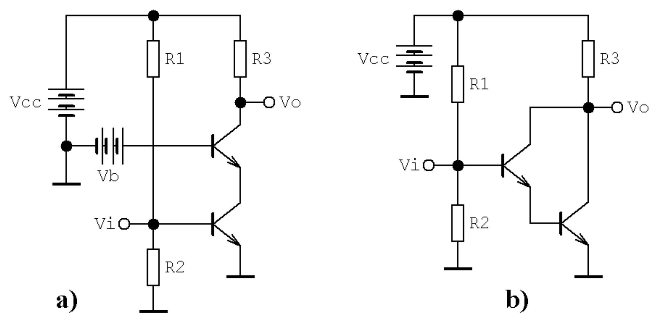
Appendix A. Common Function of Two-Transistor Cascoded Amplifier
Both cascoded amplifier and amplifier with Darlington’s pair belong to the favorite circuit topologies. A typical example of a cascoded amplifier with resistive load is provided in Figure A1. It is a specific interconnection of either two bipolar or two unipolar transistors. The first transistor, driven by the input voltage Vi, is connected in either common-emitter or common-source topology. The second (output) stage is formed by either the common-base or common-gate connection of the transistor. The advantage of this structure is the reduction of the Miller effect and, consequently, a higher bandwidth of this circuit. In contrast to the investigated “chaotified cascoded amplifier” the stability of this circuit is significant, simply because little feedback is fed from output to input node.
Figure A1 also shows a resistively loaded amplifier formed by Darlington’s pair of bipolar transistors. This is an interconnection of two common-collector topologies leading to a significant boosting of current amplification. In fact, the resulting current amplification (final beta) is a product of the betas of the individual transistors. An inevitable drawback of the real circuit is the doubled base-emitter voltage required to open Darlington’s pair.
Figure A1.
Traditional topology of analyzed amplifiers, circuit is driven by the input voltage Vi while the response can be obtained at node Vo: (a) cascoded type, (b) having Darlington’s pair.
Figure A1.
Traditional topology of analyzed amplifiers, circuit is driven by the input voltage Vi while the response can be obtained at node Vo: (a) cascoded type, (b) having Darlington’s pair.
References
- Matsumoto, T. A chaotic attractor from Chua’s circuit. IEEE Trans. Circuits Syst. 1984, 31, 1055–1058. [Google Scholar] [CrossRef]
- Huang, A.; Pivka, L.; Wu, C.W.; Franz, M. Chua’s equation with cubic nonlinearity. Int. J. Bifurc. Chaos 1996, 6, 2175–2222. [Google Scholar] [CrossRef]
- Zhong, G.-Q. Implementation of Chua’s circuit with a cubic nonlinearity. IEEE Trans. Circuits Syst. I 1994, 41, 934–941. [Google Scholar] [CrossRef] [Green Version]
- Chua, L.O. Global unfolding of Chua’s circuit. IEICE Trans. Fundam. 1993, 76, 704–734. [Google Scholar]
- Bilotta, E. A Gallery of Chua Attractors; World Scientific: Singapore, 2008; 600p. [Google Scholar]
- Guzan, M. Variations of boundary surface in Chua’s circuit. Radioengineering 2015, 24, 814–823. [Google Scholar] [CrossRef]
- Spany, V.; Galajda, P.; Guzan, M.; Pivka, L.; Olejar, M. Chua’s singularities: Great miracle in circuit theory. Int. J. Bifurc. Chaos 2010, 20, 2993–3006. [Google Scholar] [CrossRef]
- Kuznetsov, N.V.; Kuznetsova, O.A.; Leonov, G.A.; Mokaev, T.N.; Stankevich, N.V. Hidden attractors localization in Chua circuit via the describing function method. IFAC-PapersOnLine 2017, 50, 2651–2656. [Google Scholar] [CrossRef]
- Galias, Z. Positive topological entropy of Chua’s circuit: A computer assisted proof. Int. J. Bifurc. Chaos 1997, 7, 331–349. [Google Scholar] [CrossRef] [Green Version]
- Tsay, S.-C.H.; Huang, C.H.-K.; Chen, W.-T.; Wu, Y.-R. Synchronization of Chua chaotic circuits with application to the bidirectional secure communication systems. Int. J. Bifurc. Chaos 2005, 15, 605–616. [Google Scholar] [CrossRef]
- Itoh, M. Spread spectrum communication via chaos. Int. J. Bifurc. Chaos 1999, 9, 155–213. [Google Scholar] [CrossRef]
- Endo, T.; Chua, L.O. Chaos from phase-locked loops. IEEE Trans. Circuits Syst. 1988, 35, 987–1003. [Google Scholar] [CrossRef]
- Fossas, E.; Olivar, G. Study of chaos in the buck converter. IEEE Trans. Circuits Syst. 1996, 43, 13–25. [Google Scholar] [CrossRef] [Green Version]
- Bernardo, M.; Tse, C.H.-K. Chaos in Power Electronics; World Scientific Series: Singapore, 2002; pp. 317–340. [Google Scholar] [CrossRef]
- Kennedy, M.P. Chaos in the Colpitts oscillator. IEEE Trans. Circuits Syst. 1994, 41, 771–774. [Google Scholar] [CrossRef]
- Kvarda, P. Chaos in Hartley’s oscillator. Int. J. Bifurc. Chaos 2002, 12, 2229–2232. [Google Scholar] [CrossRef]
- Kilic, R.; Yildrim, F. A survey of Wien bridge-based chaotic oscillator: Design and experimental issues. Chaos Solitons Fractals 2008, 38, 1394–1410. [Google Scholar] [CrossRef]
- Keuninckx, L.; Van der Sande, G.; Danckaert, J. Simple two-transistor single-supply resistor-capacitor chaotic oscillator. IEEE Trans. Circuits Syst. II 2015, 62, 891–895. [Google Scholar] [CrossRef]
- Rajagopal, K.; Li, C.H.; Nazarimehr, F.; Karthikeyan, A.; Duraisamy, P.; Jafari, S. Chaotic dynamics of modified Wien bridge oscillator with fractional order memristor. Radioengineering 2019, 28, 165–174. [Google Scholar] [CrossRef]
- Petrzela, J. Multi-valued static memory cell with resonant tunneling diodes as natural source of chaos. Nonlinear Dyn. 2018, 94, 1867–1887. [Google Scholar] [CrossRef]
- Petrzela, J. On the existence of chaos in the electronically adjustable structures of state variable filters. Int. J. Circuit Theory Appl. 2016, 44, 1779–1797. [Google Scholar] [CrossRef]
- Kvarda, P. Identifying the deterministic chaos by using the Lyapunov exponents. Radioengineering 2000, 10, 38–40. [Google Scholar]
- Kvarda, P. Identifying the deterministic chaos by using the Lorenz maps. Radioengineering 2000, 9, 32–33. [Google Scholar]
- Minati, L.; Frasca, M.; Oswiecimka, P.; Faes, L.; Drozd, S. Atypical transistor-based chaotic oscillators: Design, realization, and diversity. Chaos 2017, 27, 073113. [Google Scholar] [CrossRef]
- Silva-Juarez, A.; Tlelo-Cuautle, E.; Gerardo de la Fraga, L.; Li, R. Optimization of the Kaplan-Yorke dimension in fractional-order chaotic oscillators by metaheuristic. Appl. Math. Comput. 2021, 394, 125831. [Google Scholar] [CrossRef]
- Jafari, S.; Sprott, J.C.; Pham, V.-T.; Reza Hashemi Golpayegani, M. A new cost function for parameter estimation of chaotic systems using return maps as fingerprints. Int. J. Bifurc. Chaos 2014, 24, 1450134. [Google Scholar] [CrossRef]
- Petrzela, J. New chaotic oscillator derived from class C single transistor-based amplifier. Math. Probl. Eng. 2020, 2020, 2640629. [Google Scholar] [CrossRef]
- Petrzela, J. Chaotic and hyperchaotic self-oscillations of lambda diode composed by generalized bipolar transistors. Appl. Sci. 2021, 11, 3326. [Google Scholar] [CrossRef]
- Petrzela, J. Hyperchaotic self-oscillations of two-stage class C amplifier with generalized bipolar transistors. IEEE Access 2021, 9, 62182–62194. [Google Scholar] [CrossRef]
- Valencia-Ponce, M.A.; Tlelo-Cuautle, E.; Gerrardo de la Fraga, L. Estimating the highest time-step in numerical methods to enhance the optimization of chaotic oscillators. Mathematics 2021, 9, 1938. [Google Scholar] [CrossRef]
- Zhang, F.; Zhang, G.; Lin, D.; Sun, X.-K. Global attractive sets of a novel bounded chaotic system. Neural Comput. Appl. 2014, 25, 1177–1183. [Google Scholar] [CrossRef]
- Zhang, F. Analysis of a Lorenz-like chaotic system by Lyapunov functions. Complexity 2019. [Google Scholar] [CrossRef]
- Ul Abadin Zafar, Z.; Sene, N.; Rezazadeh, H.; Esfandian, N. Tangent nonlinear equation in context of fractal fractional operators with nonsingular kernel. Math. Sci. 2021, 10, 1–11. [Google Scholar] [CrossRef]
- Zhou, M.-X.; Ravi Kanth, A.S.V.; Aruna, K.; Raghavendar, K.; Rezazadeh, H.; Inc, M.; Aly, A.A. Numerical solutions of time fractional Zakharov-Kuznetsov equation via natural transform decomposition method with nonsingular kernel derivatives. J. Funct. Spaces 2021, 2021, 1–17. [Google Scholar] [CrossRef]
- Petras, I. Tuning and implementation methods for fractional-order controllers. Fract. Calc. Appl. Anal. 2012, 15, 282–303. [Google Scholar] [CrossRef]
- Kadlcik, L.; Horsky, P. A low-dropout voltage regulator with a fractional-order control. Radioengineering 2016, 25, 312–320. [Google Scholar] [CrossRef]
- Yao, J.; Wang, K.; Huang, P.; Chen, L.; Machado, J.T. Analysis and implementation of fractional-order chaotic system with standard components. J. Adv. Res. 2020, 25, 97–109. [Google Scholar] [CrossRef]
- Petrzela, J. Fractional-order chaotic memory with wideband constant phase elements. Entropy 2020, 22, 422. [Google Scholar] [CrossRef] [Green Version]
- Kartci, A.; Herencsar, N.; Machado, J.T. History and progress of fractional-order element passive emulators: A review. Radioengineering 2020, 29, 296–304. [Google Scholar] [CrossRef]
- Valencia-Ponce, M.A.; Castaneda-Avina, P.R.; Tlelo-Cuautle, E.; Carbajal-Gomez, V.H.; Gonzalez-Diaz, V.R.; Sandoval-Ibarra, Y.; Nunez-Perez, J.-C. CMOS OTA-based filters for designing fractional-order chaotic oscillators. Fractal Fract. 2021, 5, 122. [Google Scholar] [CrossRef]
- Kapoulea, S.; Psychalinos, C.; Elwakil, A.S. FPAA-based realization of filters with fractional Laplace operators of different orders. Fractal Fract. 2021, 5, 218. [Google Scholar] [CrossRef]
- Mohamed, S.M.; Sayed, W.S.; Said, L.A.; Radwan, A.G. Reconfigurable FPGA realization of fractional-order chaotic systems. IEEE Access 2021, 9, 89376–89389. [Google Scholar] [CrossRef]
- Sprott, J.C. A proposed standard for the publication of new chaotic systems. Int. J. Bifurc. Chaos 2011, 21, 2391–2394. [Google Scholar] [CrossRef] [Green Version]
- Itoh, M. Synthesis of electronic circuits for simulating nonlinear dynamics. Int. J. Bifurc. Chaos 2001, 11, 605–653. [Google Scholar] [CrossRef]
- Petrzela, J.; Gotthans, T.; Guzan, M. Current-mode network structures dedicated for simulation of dynamical systems with plane continuum of equilibrium. J. Circuits Syst. Comput. 2018, 27, 1830004. [Google Scholar] [CrossRef]
- Valencia-Ponce, M.A.; Tlelo-Cuautle, E.; Gerrardo de la Fraga, L. On the sizing of CMOS operational amplifiers by applying many-objective optimization algorithms. Electronics 2021, 10, 3148. [Google Scholar] [CrossRef]
- Dudkowski, D.; Jafari, S.; Kapitaniak, T.; Kuznetsov, N.V.; Leonov, G.A.; Prasad, A. Hidden attractors in dynamical systems. Phys. Rep. 2016, 637, 1–50. [Google Scholar] [CrossRef]
- Pham, V.-T.; Volos, C.H.; Jafari, S.; Kapitaniak, T. Coexistence of hidden attractors in a novel no-equilibrium system. Nonlinear Dyn. 2017, 87, 2001–2010. [Google Scholar] [CrossRef]
Figure 1.
Simplified schematic of analyzed networks: (a) concept of driven cascaded resonant stage with non-ideal generalized bipolar transistors, (b) isolated circuit dedicated for calculations with equivalent models of generalized transistors.
Figure 1.
Simplified schematic of analyzed networks: (a) concept of driven cascaded resonant stage with non-ideal generalized bipolar transistors, (b) isolated circuit dedicated for calculations with equivalent models of generalized transistors.

Figure 2.
Simplified schematic of analyzed networks: (a) concept of driven resonant Darlington’s stage with non-ideal GBT (non-integrated, discrete form of implementation), (b) isolated circuit with equivalent models of generalized transistors.
Figure 2.
Simplified schematic of analyzed networks: (a) concept of driven resonant Darlington’s stage with non-ideal GBT (non-integrated, discrete form of implementation), (b) isolated circuit with equivalent models of generalized transistors.

Figure 3.
Cascoded resonant amplifier considered as fourth order dynamical system, parameter case and , generated strange attractor projected in: (a) subspace v1-v2-v3, (b) subspace v2-v3-iL, and (c) subspace v1-iL-v3. Sensitivity analysis: (d) group of 104 initial conditions with uniform distribution, (e) evolution of states for different time scales, see text for details. System case and , generated the strange attractor projected in: (f) subspace v1-v2-v3, (g) subspace v2-v3-iL, and (h) subspace v1-iL-v3, associated sensitivity analysis: (i) evolution of states for different time scales. System case and , generated strange attractor projected in: (j) subspace v1-v2-v3, (k) subspace v2-v3-iL, and (l) subspace v1-iL-v3, associated sensitivity analysis: (m) evolution of states for different time scales.
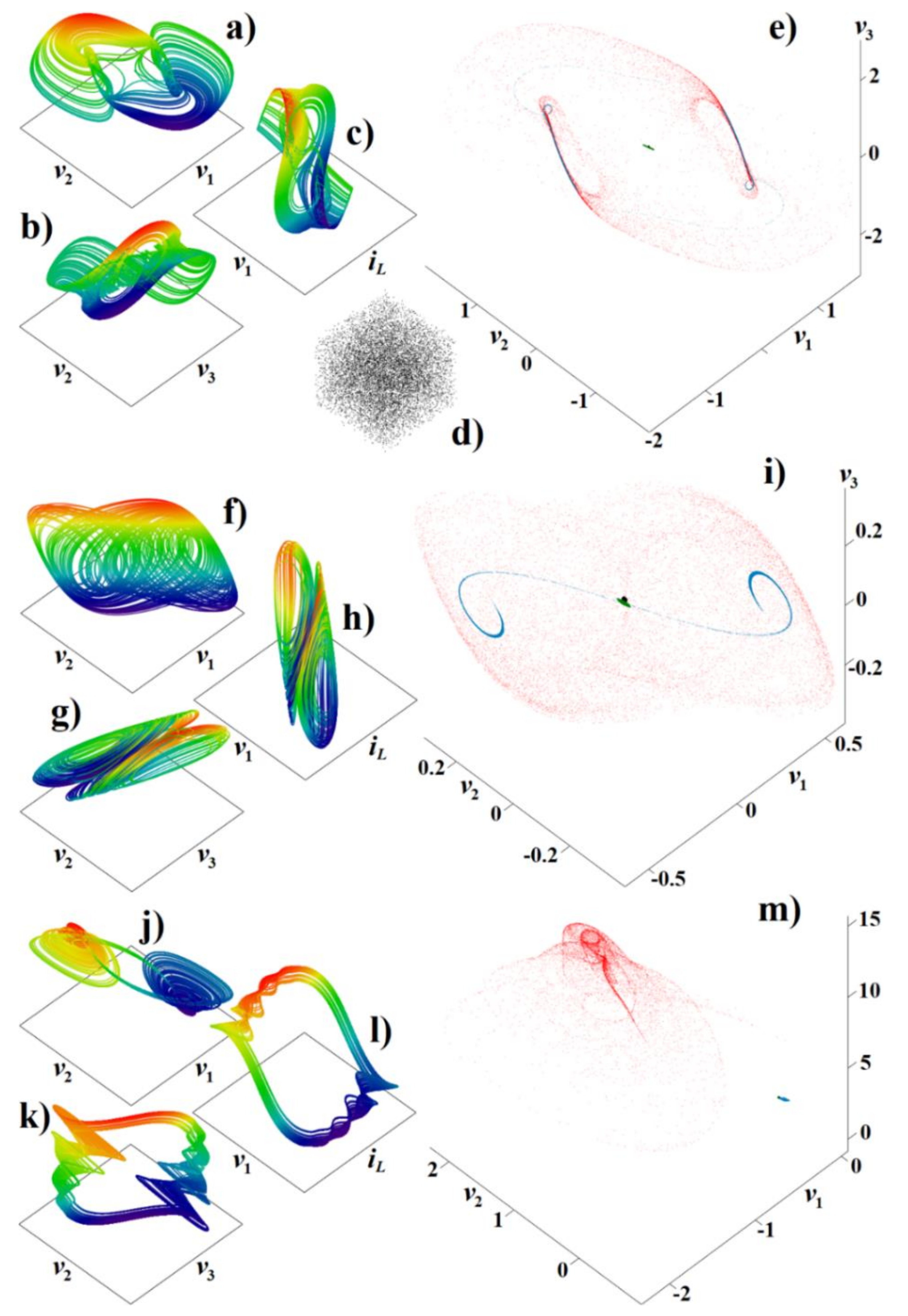
Figure 4.
Cascoded resonant amplifier considered as a fourth order autonomous dynamical system. Kinetic energy distribution over the state space visualized in all available plane projections and for: (a–f) parameter set , , (g–l) , , and (m–q) , . In each plot, only two state variables are swept while remaining state variables are kept zero. See text for the better understanding of the individual plots.
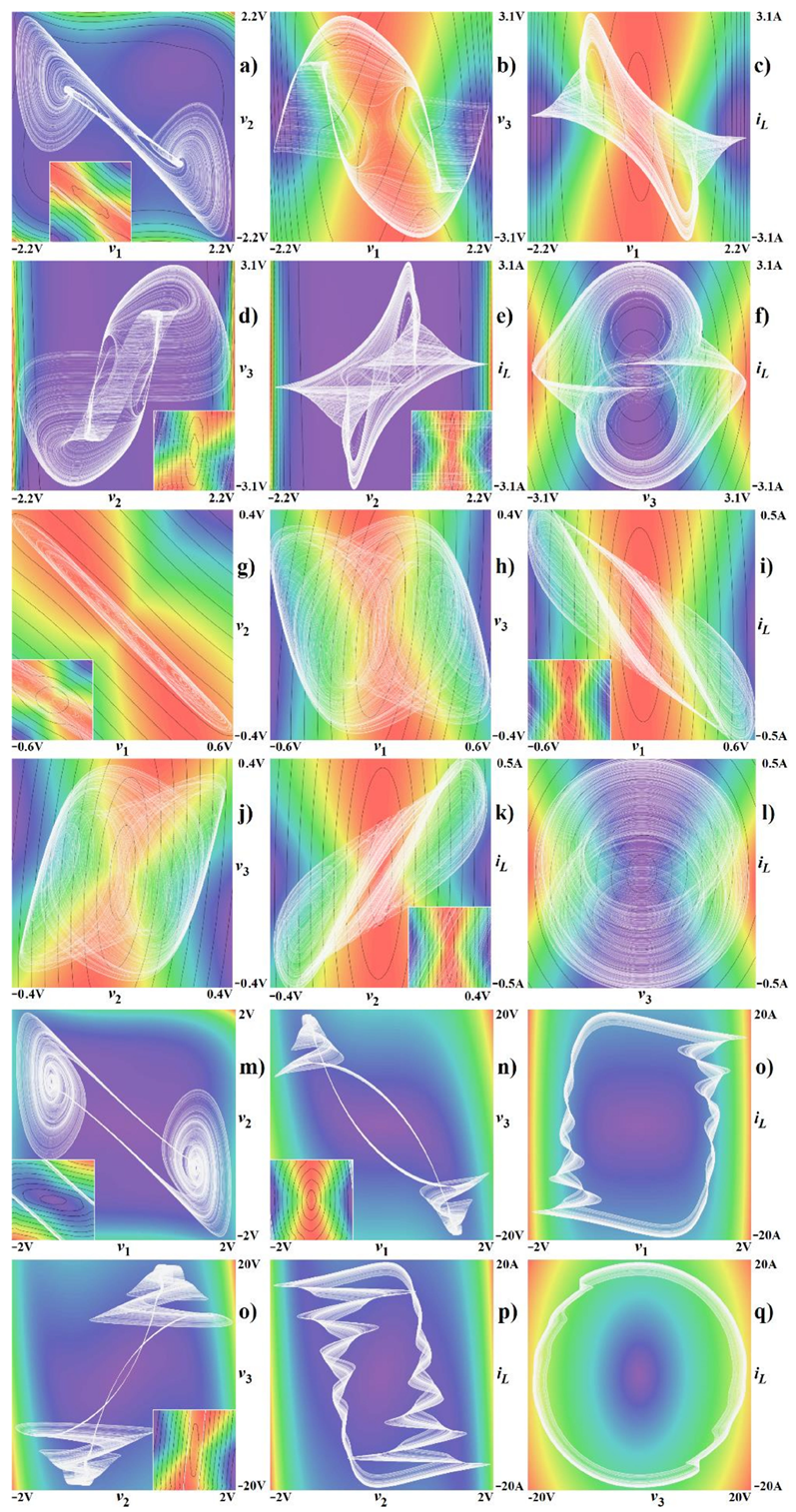
Figure 5.
Cascoded resonant amplifier assumed as fourth order dynamical system. Colored basins of attraction, the plane fragments are defined as: (a) v1 vs. v2, (b) v1 vs. v3, (c) v1 vs. iL, (d) v2 vs. v3, (e) v2 vs. iL, and (f) v3 vs. iL. The rest of plots represent zoomed areas focused on the interesting boundaries between different system solutions. Magnified areas have following ranges of the state variables: (g) v1 ∈ (−3, −2) V, v2 ∈ (2, 3) V, (h) v1 ∈ (−2.35, −2.32) V, v2 ∈ (2.34, 2.37) V, (i) v1 ∈ (−2343, −2340) mV, v2 ∈ (2354, 2357) mV, (j) v1 ∈ (0.8, 2) V, v3 ∈ (2, 3.2) V.

Figure 6.
Cascoded resonant amplifier, fourth order system. Rainbow-scaled surface-contour plot of the largest LE, parameter step varies such that each plot contains equally spaced grid of 101 × 101 = 10,201 points. Zooming procedure: (a)-(b)-(c)-(d), (a)-(e)-(f)-(g), (a)-(h)-(m), (a)-(h)-(i)-(j).
Figure 6.
Cascoded resonant amplifier, fourth order system. Rainbow-scaled surface-contour plot of the largest LE, parameter step varies such that each plot contains equally spaced grid of 101 × 101 = 10,201 points. Zooming procedure: (a)-(b)-(c)-(d), (a)-(e)-(f)-(g), (a)-(h)-(m), (a)-(h)-(i)-(j).

Figure 7.
Cascoded resonant amplifier analyzed as third order dynamical system: (a) turbulent chaotic attractor evolved for the initial conditions x0 = (2.3, −3, −8)T, (b) mirrored attractor for initial conditions x0 = (−2.3, 3, 8)T, (c) system sensitivity to changes of initial conditions (see text for details). Basins of attraction for both mirrored strange attractors: (d,e), unbounded solution is marked by red color, evolution toward the strange attractor is denoted by blue color. Mutual position between mirrored attractors: (f). For further details, consult corresponding paragraph in main text.

Figure 8.
Analysis of isolated resonant amplifier with Darlington-type cell, fourth order dynamical system: (a) subspace v1-v2-v3, (b) subspace v1-v2-iL, (c) subspace v2-v3-iL, (d) hypercube of randomly generated sets of the initial conditions, (e) short-time system evolution. See text for clarification of individual plots.
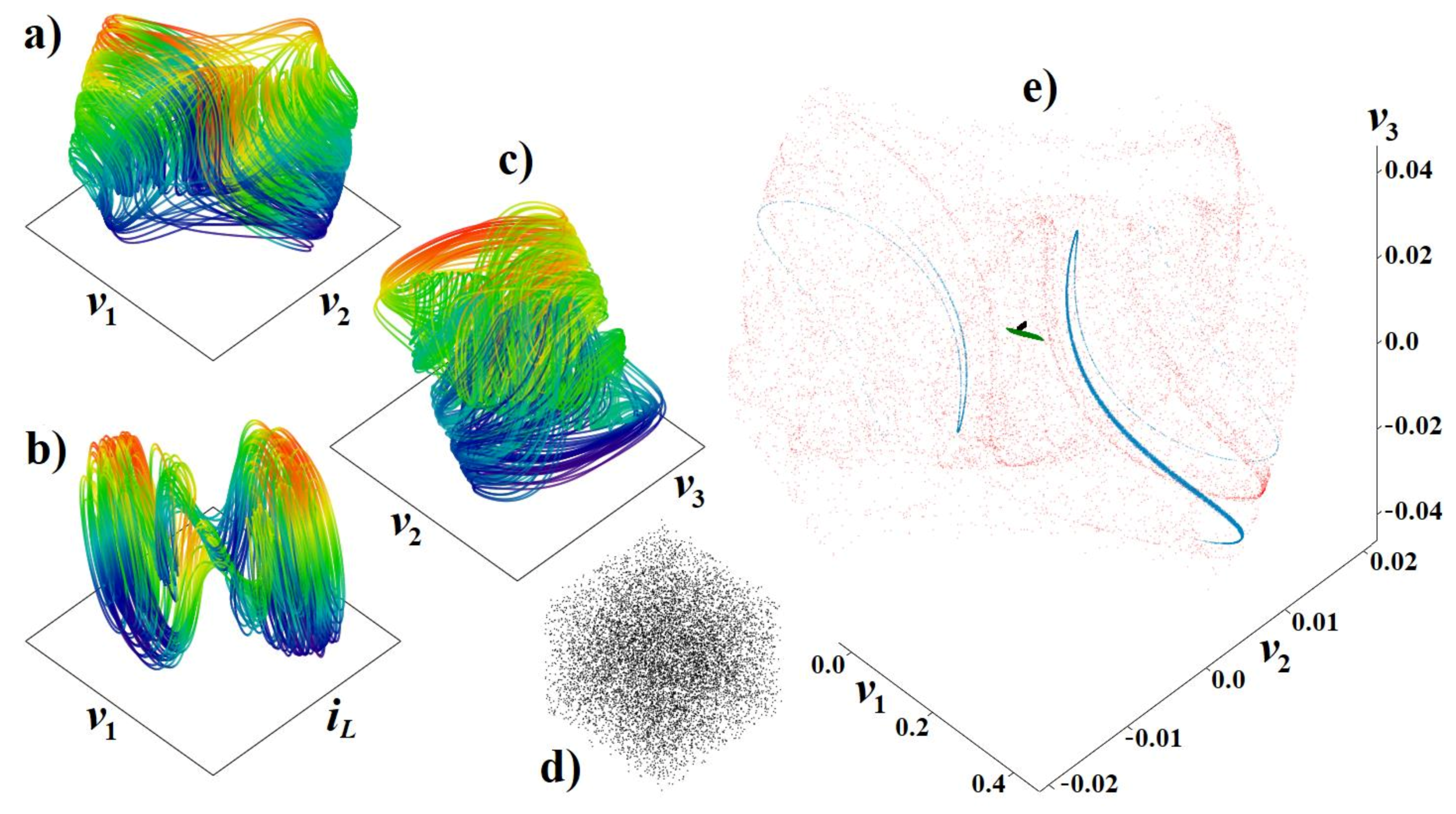
Figure 9.
For both Darlington-type composites, calculation of the kinetic energy, the static energy loss and divergency of vector field visualized in v1-v2 plane (rainbow scaling legend is included). Fourth order system (11) with value set (22) we obtained: (a) dynamic energy loss for v3 = 0 V and iL = 0 A, (b) static energy loss for v3 = 0 V and iL = 0 A, (c) divergency for v3 = 0 V and iL = 0 A. For third order system (16) with values (24) we get: (d) dynamic energy for v3 = 0 V, (e) static energy loss for v3 = 0 V, (f) vector field divergency for v3 = 0 V. Energies are related to 1 s time instance.
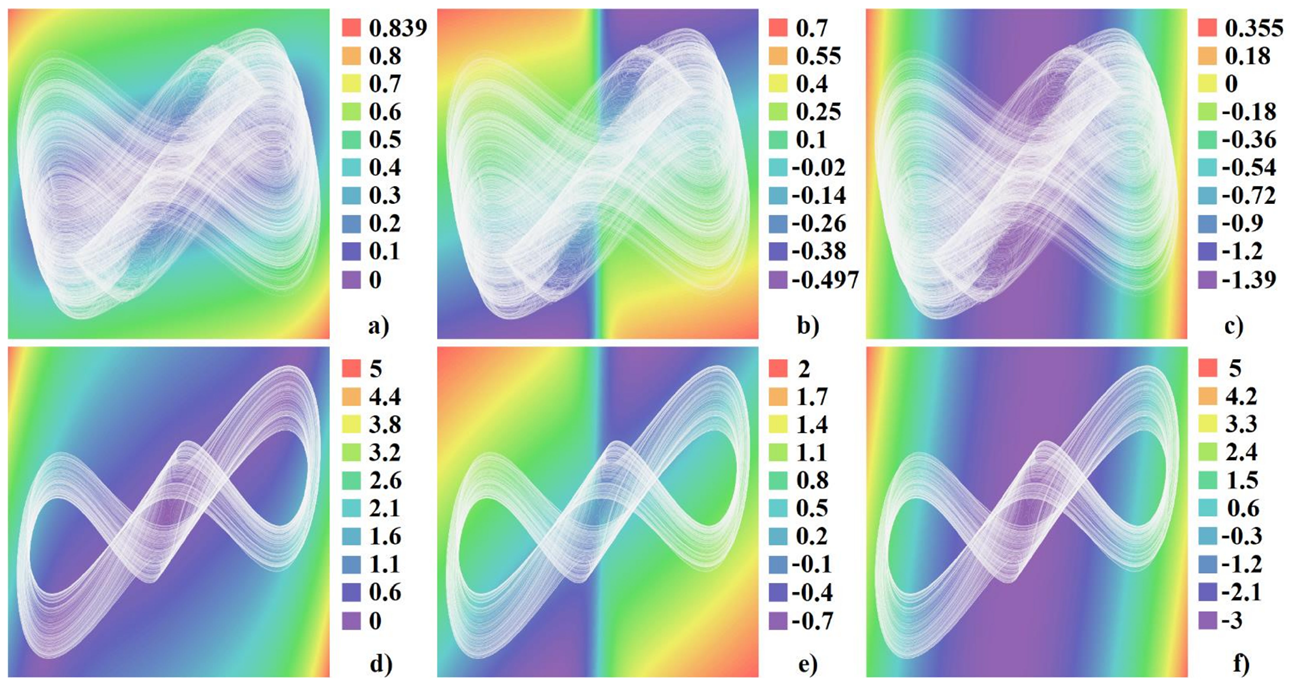
Figure 10.
Resonant amplifier with Darlington-type cell, analysis of fourth order system, colored basins of attraction. See text for clarification of the individual plots.
Figure 10.
Resonant amplifier with Darlington-type cell, analysis of fourth order system, colored basins of attraction. See text for clarification of the individual plots.

Figure 11.
Resonant amplifier with Darlington-type composite, fourth order system considered for analysis. Rainbow-scaled composition of contour plots of two LE, circled areas combined filled with orange or red color denote parameter configurations leading to distinguished hyperchaotic motion (positive value of both first and second LE), unified color scale legend for LLE is included.

Figure 12.
Resonant amplifier with Darlington-type topology, third order autonomous dynamical system is considered for analysis. Perspective 3D views (black trajectory) on the typical strange attractor including individual plane projections (orange color for v1 vs. v2, blue color denotes v1 vs. v3 and green color marks v2 vs. v3) for: (a) , (b) , (c) sensitivity of system solution to the changes of the initial conditions, (d) group of 104 initial conditions generated by following the normal distribution, (e) rainbow-scaled contour-surface plot of the largest LE calculated for parameter range and color legend provided.
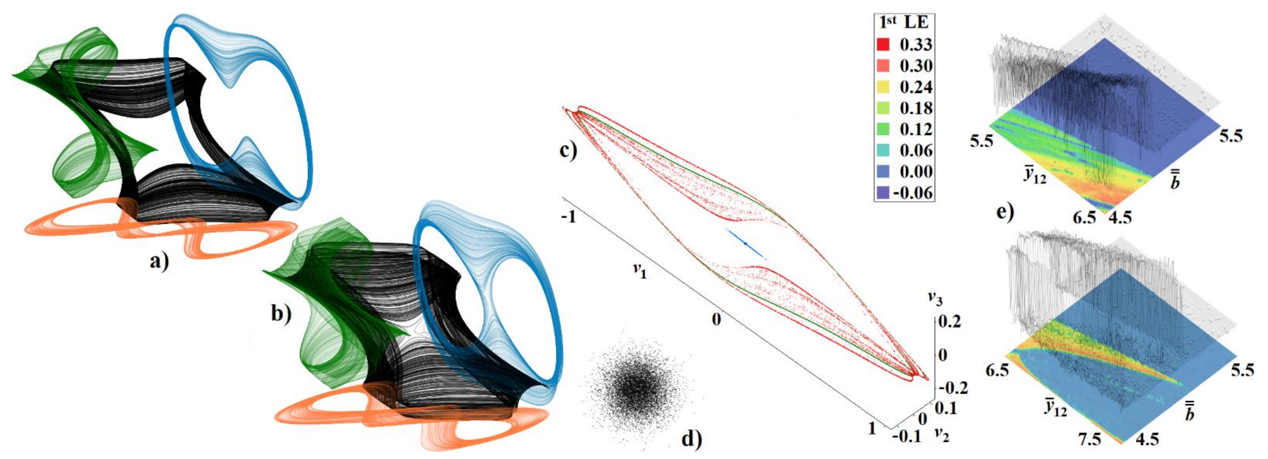
Figure 13.
Circuitry realization of cascoded amplifier: (a) with resonant load implemented using analog computer concept, (b) with resistive load implemented using trans-conductance cells.
Figure 13.
Circuitry realization of cascoded amplifier: (a) with resonant load implemented using analog computer concept, (b) with resistive load implemented using trans-conductance cells.

Figure 14.
Selected oscilloscope screenshots captured during measurement of cascoded amplifier.
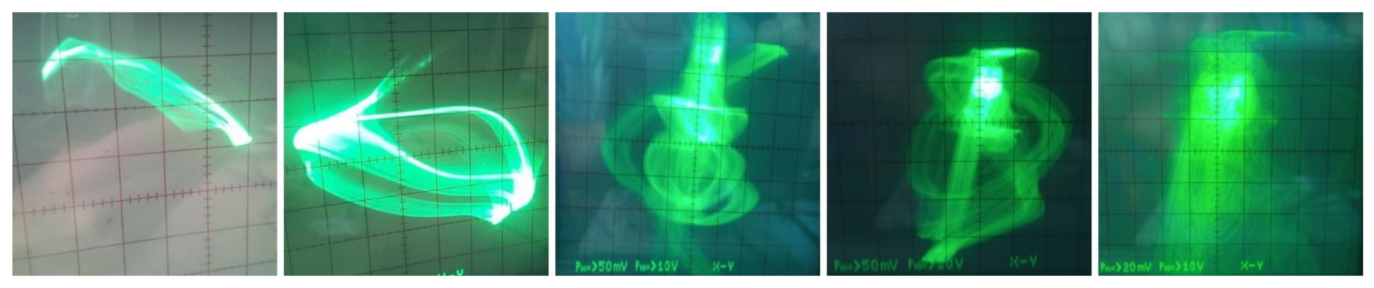
Figure 15.
Darlington’s stage with resistive load: (a) analog computer-based circuit realization, (b) plane projection v1 vs. v2 (blue color) and v1 vs. v3 (red color), (c) frequency spectrum of chaotic signal v1 (blue color) and v3 (red color).
Figure 15.
Darlington’s stage with resistive load: (a) analog computer-based circuit realization, (b) plane projection v1 vs. v2 (blue color) and v1 vs. v3 (red color), (c) frequency spectrum of chaotic signal v1 (blue color) and v3 (red color).
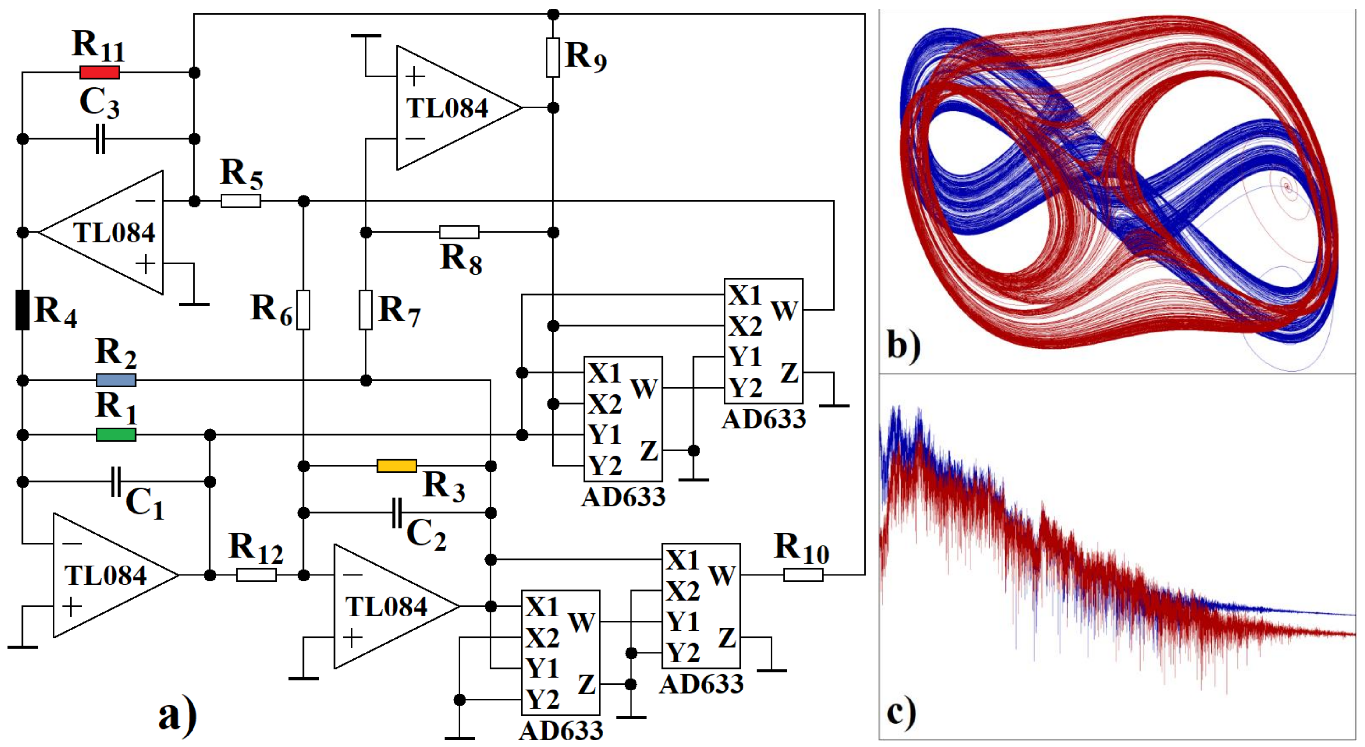
Figure 16.
Darlington’s stage having output opened (that is infinite load resistance), 1D bifurcation diagram for narrow range of: (a) black resistor, (b) green resistor.
Figure 16.
Darlington’s stage having output opened (that is infinite load resistance), 1D bifurcation diagram for narrow range of: (a) black resistor, (b) green resistor.

Publisher’s Note: MDPI stays neutral with regard to jurisdictional claims in published maps and institutional affiliations. |
© 2022 by the authors. Licensee MDPI, Basel, Switzerland. This article is an open access article distributed under the terms and conditions of the Creative Commons Attribution (CC BY) license (https://creativecommons.org/licenses/by/4.0/).
Share and Cite
MDPI and ACS Style
Petrzela, J.; Rujzl, M. Chaotic Oscillations in Cascoded and Darlington-Type Amplifier Having Generalized Transistors. Mathematics 2022, 10, 532. https://doi.org/10.3390/math10030532
AMA Style
Petrzela J, Rujzl M. Chaotic Oscillations in Cascoded and Darlington-Type Amplifier Having Generalized Transistors. Mathematics. 2022; 10(3):532. https://doi.org/10.3390/math10030532
Chicago/Turabian StylePetrzela, Jiri, and Miroslav Rujzl. 2022. "Chaotic Oscillations in Cascoded and Darlington-Type Amplifier Having Generalized Transistors" Mathematics 10, no. 3: 532. https://doi.org/10.3390/math10030532
Note that from the first issue of 2016, this journal uses article numbers instead of page numbers. See further details here.