

Analysis of the Stability and Optimal Control Strategy for an ISCR Rumor Propagation Model with Saturated Incidence and Time Delay on a Scale-Free Network

Business School, University of Shanghai for Science and Technology, Shanghai 200093, China
*
Author to whom correspondence should be addressed.
Mathematics 2022, 10(20), 3900; https://doi.org/10.3390/math10203900
Submission received: 10 August 2022
/
Revised: 7 October 2022
/
Accepted: 9 October 2022
/
Published: 20 October 2022
Abstract
:The spread of rumors in the era of new media poses a serious challenge to sustaining social order. Models regarding rumor propagation should be proposed in order to prevent them. Taking the cooling-off period into account in this paper, a modified ISCR model with saturated incidence and time delay on a scale-free network is introduced. The basic reproduction number , which does not depend on time delay , is given by simple calculation. The stability of the rumor-free and rumor-endemic equilibrium points is proved by constructing proper Lyapunov functions. The study of the ISCR rumor-spreading process acquires an understanding of the impact of many factors on the prevalence of rumors. Then, the optimal control strategy for restraining rumors is studied. Numerous sensitivity studies and numerical simulations are carried out. Based on the saturated incidence and time delay, results indicate that the effect of time delay plays a significant part in rumor propagation on a scale-free network.
1. Introduction
Rumors diffusion is defined as unconfirmed elaborations or annotations related to shared interests and is widely spread through different channels [1]. With the flexibility of social media development providing a low threshold, thousands of individuals, and real-time dissemination of information in our daily life, people can be exposed to a large amount of data more and more conveniently. However, some of the information that is not screened can be the opposite of the facts, and this has greatly influenced people’s lives. Spreading rumors is a common instance of social communication and is important to social life. Rumors diffusion has a negative impact on society and causes panic among the population. The rapid spread and the tremendous social trouble of rumors have brought considerable costs to authority supervision. Studying the spreading process of rumors can bring insight into the influence of different factors and significantly lower the adverse effects of rumors to work out better control strategies to restrain rumor propagation [2]. Therefore, enhancing the investigations of the rumor dissemination mechanism can lead to curbing rumor propagation by rapid government and media involvement.
There are many similarities between rumors diffusion and the transmission of disease in the principle of propagation and the similarity of population classification. Therefore, many scholars’ analyses of rumor propagation were based on research on disease transmission. In the early stages, the D-K model, a typical rumor propagation model was studied by Daley and Kendall [3]. In this model, individuals are divided into three categories: people who hear nothing of the rumor, people who transmit it, and people who hear it but will never share it. Based on the D-K model, Maki and Thomson proposed the M-K model, which assumes that a spreader can change into a stifler who stops spreading the rumor [4]. Many extended rumor propagation models have been proposed and studied based on these two models [5,6,7]. Kawachi et al. improved a rumor propagate model with multiple contact interactions that can prove the rumor recursion [5]. Yao et al. studied different contact statuses for other users considering some realistic constraint conditions [6]. Zhou et al. proposed a new SCIR model that considers that trust affects the level of empathy [7]. However, these rumor propagations are not appropriate in a social network environment without considering the influence of complex network topologies, such as regular networks, random networks, small-world networks, and scale-free networks [8,9,10,11]. Zanette firstly proposed the dynamic behavior of rumor-spreading on small-world networks and acquired the network topologies that had a remarkable impact on the propagation threshold [8]. Moreno et al. developed the mean-field theory on the scale-free network [9]. Li et al. proposed a novel I2S2R rumor model with a multilingual environment education process on heterogeneous networks [10]. Ai et al. improved the traditional Barabasi–Albert scale-free network and proposed a network topology model that conforms to the characteristics of sharing social networks based on the complex network theory and the actual attributes of sharing social networks [11]. These studies show that the network’s topology significantly impacts rumor propagation, and different types of networks yield different results from the propagation dynamics. As a result, research on the dynamics of complex network propagation has always been attractive, and it is also crucial for understanding how rumors spread in real network systems.
In addition, rumor propagation is influenced by many factors, such as heterogeneity of transmission and network [12,13], the hesitating mechanism [14], the memory [15], the skepticism and denial [16,17], the education or scientific knowledge [18], the latency [19], super spreading effect [20], and others [21,22]. Based on different rumor-spreading models, propagation delay is also an essential factor affecting rumor spreading. Different rumor-spreading models suggest that propagation delay is also essential to rumor diffusion. Zhu et al. established the I2S2R rumor model, incorporating time delay in both homogeneous and heterogeneous networks [23]. Guan et al. formulated a modified SHIR model with two susceptible groups and combined time delay and nonlinear incidence rate in networks with various topologies [24]. Yu et al. researched new 2I2SR rumor propagation models with and without time delay based on a multilingual environment, and a real-time optimization method that minimizes the cost of the restraining rumor is proposed to eliminate the rumor within an expected period [25]. Cheng et al. established an improved rumor-spreading model to explore the new characteristics of the rumor spreading process considering media coverage and the delay of the interactive system [26,27]. Without loss of generalization, many scholars usually assume that the spreaders directly turn to stiflers regarding the rumor model. However, these assumptions lose sight of the possibility that the rumor-spreading may undergo an incubation period, such as a cooling-off period or a calmness period, before becoming stiflers to make the rumor propagation model more realistic. Chen proposed an ILSCR rumor model with a cooling-off period [28]. Chang et al. studied a novel ISCR rumor propagation model, adding a calmness compartment to make the model more realistic [29]. These studies point to the idea that in reality, specific factors will significantly influence the process of spreading rumors, so it crucial for the research to take these factors into account, such as propagation delay, calmness compartment, and so on.
In the above studies, many models only consider the linear incidence in rumor propagation, but it is more beneficial to adopt a nonlinear incidence in reality. Wang et al. proposed a nonlinear model to represent the impact of awareness by the media report [30]. Zhu et al. proposed a rumor propagation model with a silence-forcing function, and the optimal control was discussed to reduce the frequency of rumor propagation in online social networks [31]. On the other hand, Zhu et al. discussed a 2ISR rumor model with nonlinear analysis and time delay in both homogeneous and heterogeneous networks [32]. Wang et al. studied an IS2R2 model concerning the nonlinear inhibition mechanism and designed an optimal control strategy [33]. Chen et al. investigated a novel SEIR delayed rumor model with saturation incidence on heterogeneous networks and proposed an optimal control strategy [34]. Additionally, many scholars continue to focus on the control of rumor diffusion [35,36,37,38,39]. Zhu et al. established an SIS rumor model considering targeted immunization control, acquaintance immunization control, and optimal control strategies [35]. Ding et al. proposed a hybrid control strategy, combining a continuous truth propagation method and an impulsive rumor blocking method on online social networks [36]. Li et al. developed comprehensive interventions with qualitative and quantitative analysis based on the ILRDS rumor model [37]. Liu et al. studied a dynamic quarantine defense model to improve the cost and efficiency of rumor diffusion control [38]. Yu et al. studied an I2SR rumor model with an environment event-triggered impulsive control strategy in heterogeneous networks [39]. Xia et al. proposed a new ILSR rumor-spreading model combining the incubation mechanism and general nonlinear spreading rate [40]. As well as aiming to explore the control of the spread of rumors, this paper will also put forward effective control strategies that will help control rumor propagation on a scale-free network.
The structure of this paper is arranged as follows. In Section 2, it proposes a modified ISCR model and gives the value of the basic reproduction number. In Section 3, the ISCR model including the saturated incidence rate and the time delay is further investigated. In Section 4, an optimal control problem is established and studied to control the spread of rumors. In Section 5, sensitivity analysis and some numerical simulations are carried out. In the Section 6, a brief comparison and conclusion are presented.
2. The Rumor Spreading Model
2.1. Model Formulation
As studied in [28,29], a novel ISCR model with saturated incidence and time delay on a scale-free network is proposed. The flow diagram of the model is shown in Figure 1. The total population is separated into four groups: Ignorants who have never known the rumor and consequently are open to trusting the rumor, marked by ; Spreaders who know and spread the rumor actively, marked by ; Cooled states or Cooling-off represent those who calm down before stopping the propagation of the rumor, marked by . In other words, it takes into consideration the likelihood that spreaders may go through a cooling-off phase before becoming Removes; Removes who have been contacted by the Spreaders or Cooled states but resist and do not spread it, are marked by . Each individual on the scale-free network is represented by a network node, and the connections between those nodes are what allow for rumor-spreading [9]. Taking closed and homogeneity into account, it combines the connectivity of nodes on the networks with different topologies. Let , , and be the relative densities of Ignorants, Spreaders, Cooling-off, and Removes with the degree at time , respectively. The process of the ISCR rumor propagation model is shown in Figure 1.
This is based on the mean-field theory on complex networks [41,42]. The equations of propagating dynamics can be described as follows.
where represents the incubation period. is the average number of connections between ignorant nodes and spreader nodes on a scale-free network. Expanding the time function, it obtains
where represents the conditional probability that a node with a degree will be connected to another node with the degree , namely is known as the average degree of the scale-free network. When the Ignorants are connected to the Spreaders, they will know the rumor and thus become Spreaders with a probability of and is the infection rate. represents the psychological inhibition factor, which reveals individuals’ willingness to take action to refute rumors because of available scientific knowledge both online and offline. The parameter is the recovery rate of the Spreaders under the influence of the forgetting mechanism. is the immunity rate of Spreaders with the effect of popular science education and media coverage. is the cooling-off rate of Spreaders. is the transfer rate from Cooling-off to Removes. It assumes that the immigration rate is and emigrate rate is . All the newly added nodes are classified as Ignorants and the parameters are non-negative.
According to the actual situation in the rumor propagation process, the initial conditions of the system (1) must satisfy Therefore, exists when the differential equation of the system (1) is equal to zero. In such a method, the investigation on the rumor propagation model will be centered on the positive solution.
2.2. The Basic Reproduction Number of the System (1)
System (1) always has a rumor-free equilibrium Furthermore, it assumes that the rumor-endemic equilibrium of system (1) is In light of the derivative value, the balance is zero, and it obtains
It is easy to see that are linear function with reference to , which obtains
Then, the expression of rumor-endemic equilibrium can be as shown in Equation (3).
When substituting the in Equation (5) into the time function and expanding , the formula can be defined as self-consistency equality.
is a value to the autonomous Equation (2). Moreover, the solution of the formula at has numerical results, as follows.
Therefore, the following results must be fulfilled so that for the independent Equation (6) concerning the function exists a unique non-zero solution within the range of zero and one.
The equation of the basic reproduction number can be found on account of the system (1), as follows.
3. The Stability of the Rumor Propagate Model
This section investigates the global asymptotic stability of rumor-free and rumor-endemic equilibrium utilizing the Lyapunov function and Lasalle’s invariant set principle. The stability of the rumor-endemic equilibrium point will be theoretically studied, considering the basic reproduction number is greater than 1.
Theorem 1.
If, rumor-free equilibriumof the system (1) is globally asymptotic stable. If not, it is unstable.
Proof.
The function is constructed for the sake of stability proof. It means that the function is a non-negative function on account of . The following is the construction of the Lyapunov functions.
where . In this text, it has been demonstrated that certain nodes in the system (1) have positive qualities. It can be determined that is a positive value considered in terms of , and the equation is also a positive value if . In conclusion, Lyapunov’s second theorem will satisfy the positive qualitative requirement. □
Then, and are arranged appropriately. The derivative is expanded as follows.
At the rumor-free equilibrium, every differential equation has a zero derivative. According to the first section of the Equation (11), it can be obtained with ; uniting this with the first equation of the system (1), it can acquire . It solves the original function of by giving up . It obtains . The following inequality can be obtained, , since the first section of the equation is negative. On account of , it’s obvious that . Therefore, it is concluded that , namely, nodes of Spreaders are bounded and satisfy . Simplifying the derivative obtains on account of .
Calculating the derivative of the function to obtains the following.
Furthermore, according to Equation (2), the following relations can be obtained.
Since , the above can be given up, which obtains the as:
In Equation (2), because then . When , therefore, if , it is obvious that exists when, and only when, . This part reveals that the established Lyapunov function is a function with a positive definiteness, and the derivative is negative. Thus, in terms of LaSalle’s invariance principle, rumor-free equilibrium can be globally asymptotically stable when . If not, it is unstable. Theorem 1 is proved.
Theorem 2.
If, or any non-negative time delay, it exists a unique rumor-endemic equilibriumthat is globally asymptotically stable.
Proof.
When , it considers that the rumor-endemic equilibrium point of the system is to demonstrate its stability. Considering the rumor-endemic equilibrium of system (1) to establish the Lyapunov function and is as follows
where , the function is greater than 0. Thus, and are both greater than zero. Following is a definition of the Lyapunov function . □
By employing the derivative of for and substituting the system (1) into the function (16), one obtains
Since , substituting the system equilibrium point into the function (16) can also be expressed as follows.
Then, the derivative of the function concerning is employed. It obtains
Furthermore, according to (16), it can obtain the expression of as
where, and are a part of the function . According to is always positive; thus, namely, these four functions are all less than zero.
Define , it obtains
where, and support the stated hypothesis in Reference [43]. . Therefore, it meets when, and only when, the system (1) satisfies the rumor-endemic equilibrium . In summary, the rumor-endemic equilibrium point of the system is globally asymptotically stable for any if on account of LaSalle’s invariance principle of the time-delay system [44]. Namely, no matter the Spreaders’ initial density, the rumor will eventually stabilize, and then the rumors will become prevalent.
As a result, for any non-negative time delays, if , the rumor-endemic equilibrium is globally asymptotic stable, which provides tenable forever.
4. Optimal Control Strategy for Rumor Propagation
Since adopting optimal control strategies to control rumor propagation may bring inevitable expenses in reality, the limitation of resources has to be considered. This section intends to acquire an optimal rumor propagation control strategy with saturated incidence and time delay. In system (1), there exist state variables , , , and . A control variable is introduced, which can turn with the help of a media campaign.
In this section, optimized control solutions are suggested to prevent the spread of rumors and lower the cost of controlling social media platforms. The minimum principle of Pontryagin is employed to determine the most effective control solution [45]. Therefore, a control variable is employed to express the function of the control strategy for . Next, the definition of a valid control set follows:
In the system (1), there are five state variables, According to the optimal control strategies, the control variable can control the variation, in which turns into . Namely, the percentage of Spreaders will turn into Removes. Furthermore, stands for the range of values for the recovery rate. The maximum control range is for all rumor-spreading. Therefore, to compress the objective function, an optimal control problem is taken into account.
The controlled system can be obtained by
where is all positive parameters. is set as a trade-off factor. The square of the control variable shows the significance of the remove scale effect. To acquire the optimal value, the Lagrangian function is defined as.
The control system’s Hamiltonian function is defined as follows.
where is an adjoint function to be determined.
Theorem 3.
In the optimal control system (30), an optimal controlmakingexists with initial conditions.
Proof.
The control and state variables in this minimization problem satisfy the target function’s essential convexity for being non-negative. □
represents the control spaces.
is a convex closed function, and the control system is bounded [45]. Additionally, the integrand is convex for control . It exits positive constants , and that make , meaning that the optimal control is in effect.
The maximum principle of Pontryag is applicable to the Hamiltonian function to acquire the optimal values.
If is the optimal solution to the control strategy, it exists a nontrivial vector function that satisfies the equilibrium as follows.
the following value range for the optimal control approach is obtained.
Theorem 4.
Supposeandare the optimal solutions with respect to the optimal control variablein the optimal control system (22), where,,,, and.
The adjoint variables meet
with conditions It can obtain the optimal control with the following form.
Proof.
To identify the adjoint function, the differential equation of Hamiltonian (26) concerning is adopted, and , and are substituted to acquire the first adjoint function’s expression as follows. □
The second adjoint function’s expression is as follows.
The third adjoint function’s expression is as follows.
The fourth adjoint function’s expression is as follows.
According to the conditions of (38), is established. Furthermore, it obtains
It is equivalent to
The optimal control of recovery variables has already been established. Equation (23) expands the adjoint function’s specific form, and the equation provides the following optimal control approach.
From the above discussion, the optimality strategy is built up. Due to the uncertainty of the actual situation, obtaining an effective control strategy can solve a series of practical problems
5. Numerical Simulations
This section provides some numerical simulations to support and extend the main theoretical results on a scale-free network with , where the parameter represents the smallest degree of the network nodes, and the parameter is the power-law variable [9]. Suppose , and the number of the nodes on the scale-free network is , define . Moreover, the average degree of all nodes is computed as . According to the general law of rumor propagation, there exist the initial values of the system to investigate the contents of this section in more detail.
5.1. Dynamical Behavior of System (1) on the Scale-Free Network
The basic reproduction number in system (1) is given with the parameters . Obviously, system (1) is asymptotically stable at the rumor-free equilibrium point in Figure 2a, which indicates that the densities of Ignorants and Removes tend to a positive constant, and the densities of Spreaders and Cooling-off tend to zero, which is consistent with the conclusion of Theorem 1. The basic reproduction number in the system (1) is given with the parameters .
As Figure 2b shows, the densities of Ignorants, Spreaders, Cooling-off, and Removes can be obtained over time. It demonstrates that the change range of solution curves will gradually decrease as time goes on. That is to say, system (1) eventually tends to a stable state. Namely, for any given initial value, the densities of Ignorants and Spreaders ultimately converges to a positive constant.
To further examine the rigor of the theoretical analysis results, Figure 3 and Figure 4 compare the equilibrium conditions under their limit thresholds in system (1), respectively. Considering the evolution of the system (1) with given parameters, the basic reproduction number , and can be acquired. The variation trend of and over time is shown in Figure 3a,b, respectively. In Figure 4, the rumor-free equilibrium point is of global asymptotic stability. At the same time, Figure 4 reveals that the larger it is, the slower the system (1) approaches rumor-free equilibrium point, that is to say, rumor-spreading cannot diffuse rapidly on the scale-free network when . Similarly, considering the evolution of the system (1) with given parameters, the basic reproduction number and can be acquired. Moreover, the further evolution mechanism of and over time is shown in Figure 4a,b, respectively. If , with the gradual raising of , the density of Ignorants in the system (1) will decrease; conversely, the density of Spreaders will increase, and the level of rumor-spreading will rise accordingly, which reveals that restraining the size of the basic reproduction number is an effective path to prevent rumor propagation when the rumor occurs.
5.2. The Effect of Node Degree on Rumor Propagation
The influence of degree on rumor propagation with fixed parameters is analyzed by altering the value of . The basic reproduction number is simply calculated as . Figure 5 represents evolutions of Ignorants and Spreaders with different and , respectively. With the increase of , the density of Ignorants decreases, whereas the density of Spreaders increases. According to the simulation results, the phenomenon shown in Figure 5 occurs, since nodes with more neighbors have easier access to rumor-spreading by contacting the spreaders on the scale-free network.
5.3. The Effect of Psychological Inhibition Factor on Rumor Propagation
The basic reproduction number is defined with the fixed parameters, comparing varied densities of and in the system (1) when . From Figure 6, with the gradual growth of the psychological inhibition factor , it is worth noting that the density of Ignorants increased, whereas the density of Spreaders decreased in the process of rumor propagation. This indicates that the psychological inhibition factor can reduce the density of rumor-spreading in the system (1) and restrain the influence of rumor. Namely, the psychological inhibition factor reflects the willingness of Spreaders to take active measures to suppress the spread of rumors when related rumors diffuse.
5.4. The Effect of Time Delay
on Rumor Propagation
To explain the effect of time delay on rumor propagation, the basic reproduction number is set as and . Time evolutions impact solutions of system (1) with various as , and . From Figure 7a and Figure 8a, it is evident that time delay will restrain the Ignorants’ peak density. For the time delay increases, the density of Ignorants gradually decreases. Moreover, the time delay promotes the peak of the density of Ignorants for Figure 7b and Figure 8b. Since the time delay increases, the maximum density of Ignorants also gradually increases. This shows that as the time delay of rumor propagation increases, it takes longer to eliminate the influence of rumors, making it harder to suppress the spread of rumors. Therefore, it is necessary to boost the level of public scientific knowledge through various social networking platforms by releasing widely popular science videos or articles.
5.5. The Effect of Optimal Control Strategy on Rumor Propagation
To explain the effectiveness of the optimal control strategy, the basic reproduction number is defined with fixed parameters for the sake of simplicity. Figure 9 shows the densities of and with and without the optimal control. Compared with the system (1) without control, the density of Ignorants is more prominent, whereas the density of Spreaders is smaller in the system (37). This implies that the scale of rumor-spreading can be restrained effectively with the implementation of the control strategy.
5.6. Comparative Analysis of ISR Model and ISCR Model
The comparison model considers the ISCR model without a Cooling-off state with other parameters to remain unchanged, that is, the ISR model. The time parameters of the two models are defined as . From Figure 10a,b, it is easy to examine how Cooling-off affects Spreaders and Removes over time. The red solid line and the blue solid line in Figure 10a can be compared to show how the cooling-off affects the spread rate of rumor-spreading, the highest level of spreaders, and the amount of time it takes for spreaders to achieve stability. As is evident from Figure 10b, the final proportion of Removes in the ISCR model is smaller in contrast to the ISR model. In other words, the proportion of individuals who finally know but do not spread the rumors is also reduced, and Cooling-off affects the scale of rumor-spreading. Moreover, the system is inclined to be stable for a long time. Namely, the existence of Cooling-off in the system is long, and the influence of rumors is more significant.
6. Discussions
This paper proposed a modified ISCR model on a scale-free network. It considers adding time delay to the model to make the rumor propagation model more realistic. At the same time, it employs a function to describe the nonlinear incidence rate on the scale-free network. As increases to a certain extent, is inclined to saturate. It demonstrates the stability of steady states, namely, if , the rumor-free equilibrium is globally asymptotically stable; if , the rumor-free equilibrium is unstable, and the rumor-endemic equilibrium is globally asymptotically stable by constructing different Lyapunov functions. Furthermore, this paper has analyzed the optimal control strategy for the rumor propagation model. Finally, it has verified the previous theoretical research by several numerical simulations. Implementing a control strategy can effectively restrain the rumors spread, which has good practical significance. When associated rumors diffuse, the psychological inhibition factor represents the willingness of rumor spreaders to take positive steps to halt the spread of rumors. It is essential to increase the public’s understanding of science through social media platforms by publishing widely shared scientific knowledge, such as videos or articles.
From a realistic perspective, future work will extend and enhance the rumor-spreading model by including new variables such as media coverage [46], spatial diffusion [47], multilayered network [48], control strategies [49], and so on, which sustain the mathematical model of the rumor-spreading and make it more practical [50,51]. The stochastic rumor model, including the Lévy process, can more accurately reflect the complex rumor propagation law in the real world [52]. Additionally, the network structure can be thought of as static to some extent, encouragin us to explore the construction of dynamical networks and investigate time delay and the nonlinear dynamics of a certain rumor-spreading model with actual data.
Author Contributions
Funding acquisition, L.H.; Methodology, X.Y.; Writing—original draft, X.Y. All authors have read and agreed to the published version of the manuscript.
Funding
This work was partially supported by the Program for Professor of Special Appointment (Eastern Scholar) at Shanghai Institutions of Higher Learning, and the Project for the Natural Science Foundation of Shanghai (21ZR1444100), and the Project for the National Natural Science Foundation of China (72174121, 71774111, 71871144, 71804047).
Data Availability Statement
Not applicable.
Conflicts of Interest
The authors declare no conflict of interest.
References
- Yu, Z.; Lu, S.; Wang, D.; Li, Z. Modeling and analysis of rumor propagation in social networks. Inf. Sci. 2021, 580, 857–873. [Google Scholar] [CrossRef]
- Cui, Y.; Ni, S.; Shen, S.; Wang, Z. Modeling the dynamics of information dissemination under disaster. Phys. A Stat. Mech. Its Appl. 2019, 537, 122822. [Google Scholar] [CrossRef]
- Daley, D.J.; Kendall, D.G. Epidemics and Rumours. Nature 1964, 204, 1118. [Google Scholar] [CrossRef] [PubMed]
- Maki, D.P.; Maki, D.P.; Mali, D.; Thompson, M.; Thompson, M. Mathematical Models and Applications: With Emphasis on the Social, Life, and Management Sciences; Prentice Hall: Hoboken, NJ, USA, 1973. [Google Scholar]
- Kawachi, K.; Seki, M.; Yoshida, H.; Otake, Y.; Warashina, K.; Ueda, H. A rumor transmission model with various contact interactions. J. Theor. Biol. 2008, 253, 55–60. [Google Scholar] [CrossRef] [PubMed]
- Yao, Y.; Xiao, X.; Zhang, C.; Dou, C.; Xia, S. Stability analysis of an SDILR model based on rumor recurrence on social media. Phys. A Stat. Mech. Its Appl. 2019, 535, 122236. [Google Scholar] [CrossRef]
- Zhou, X.; Qiu, L.; Hao, T. SCIR rumor propagation model with the chord mechanism in social networks. Int. J. Mod. Phys. C 2021, 33, 2250014. [Google Scholar] [CrossRef]
- Zanette, D.H. Critical behavior of propagation on small-world networks. Phys. Rev. E 2001, 64, 050901. [Google Scholar] [CrossRef] [PubMed] [Green Version]
- Moreno, Y.; Nekovee, M.; Pacheco, A.F. Dynamics of rumor spreading in complex networks. Phys. Rev. E 2004, 69, 066130. [Google Scholar] [CrossRef] [PubMed] [Green Version]
- Li, J.; Jiang, H.; Mei, X.; Hu, C.; Zhang, G. Dynamical analysis of rumor spreading model in multi-lingual environment and heterogeneous complex networks. Inf. Sci. 2020, 536, 391–408. [Google Scholar] [CrossRef]
- Ai, S.; Hong, S.; Zheng, X.; Wang, Y.; Liu, X. CSRT rumor spreading model based on complex network. Int. J. Intell. Syst. 2021, 36, 1903–1913. [Google Scholar] [CrossRef]
- Vega-Oliveros, D.A.; Da F Costa, L.; Rodrigues, F.A. Rumor propagation with heterogeneous transmission in social networks. arXiv 2016. [Google Scholar] [CrossRef] [Green Version]
- Zhou, J.; Liu, Z.; Li, B. Influence of network structure on rumor propagation. Phys. Lett. A 2007, 368, 458–463. [Google Scholar] [CrossRef]
- Xia, L.-L.; Jiang, G.-P.; Song, B.; Song, Y.-R. Rumor spreading model considering hesitating mechanism in complex social networks. Phys. A Stat. Mech. Its Appl. 2015, 437, 295–303. [Google Scholar] [CrossRef]
- Zhao, L.; Qiu, X.; Wang, X.; Wang, J. Rumor spreading model considering forgetting and remembering mechanisms in inhomogeneous networks. Phys. A Stat. Mech. Its Appl. 2013, 392, 987–994. [Google Scholar] [CrossRef]
- Sun, X.-L.; Wang, Y.-G.; Cang, L.-Q. Correlation and trust mechanism-based rumor propagation model in complex social networks. Chin. Phys. B 2022, 31, 050202. [Google Scholar] [CrossRef]
- Tian, Y.; Ding, X. Rumor spreading model with considering debunking behavior in emergencies. Appl. Math. Comput. 2019, 363, 124599. [Google Scholar] [CrossRef]
- Huo, L.; Chen, S. Rumor propagation model with consideration of scientific knowledge level and social reinforcement in heterogeneous network. Phys. A Stat. Mech. Its Appl. 2020, 559, 125063. [Google Scholar] [CrossRef]
- Liu, W.; Wu, X.; Yang, W.; Zhu, X.; Zhong, S. Modeling cyber rumor spreading over mobile social networks: A compartment approach. Appl. Math. Comput. 2018, 343, 214–229. [Google Scholar] [CrossRef]
- Zhang, Y.; Su, Y.; Weigang, L.; Liu, H. Rumor and authoritative information propagation model considering super spreading in complex social networks. Phys. A Stat. Mech. Its Appl. 2018, 506, 395–411. [Google Scholar] [CrossRef]
- Vosoughi, S.; Roy, D.; Aral, S. The spread of true and false news online. Science 2018, 359, 1146–1151. [Google Scholar] [CrossRef]
- Qiu, X.; Zhao, L.; Wang, J.; Wang, X.; Wang, Q. Effects of time-dependent diffusion behaviors on the rumor spreading in social networks. Phys. Lett. A 2016, 380, 2054–2063. [Google Scholar] [CrossRef]
- Zhu, L.; Zhou, M.; Zhang, Z. Dynamical Analysis and Control Strategies of Rumor Spreading Models in Both Homogeneous and Heterogeneous Networks. J. Nonlinear Sci. 2020, 30, 2545–2576. [Google Scholar] [CrossRef]
- Guan, G.; Guo, Z. Stability behavior of a two-susceptibility SHIR epidemic model with time delay in complex networks. Nonlinear Dyn. 2021, 106, 1083–1110. [Google Scholar] [CrossRef]
- Yu, S.; Yu, Z.; Jiang, H.; Yang, S. The dynamics and control of 2I2SR rumor spreading models in multilingual online social networks. Inf. Sci. 2021, 581, 18–41. [Google Scholar] [CrossRef]
- Cheng, Y.; Huo, L.; Zhao, L. Dynamical behaviors and control measures of rumor-spreading model in consideration of the infected media and time delay. Inf. Sci. 2021, 564, 237–253. [Google Scholar] [CrossRef]
- Cheng, Y.; Huo, L.; Zhao, L. Stability analysis and optimal control of rumor spreading model under media coverage considering time delay and pulse vaccination. Chaos Solitons Fractals 2022, 157, 111931. [Google Scholar] [CrossRef]
- Chen, G. ILSCR rumor spreading model to discuss the control of rumor spreading in emergency. Phys. A Stat. Mech. Its Appl. 2018, 522, 88–97. [Google Scholar] [CrossRef]
- Chang, Z.; Jiang, H.; Yu, S.; Chen, S. Dynamic Analysis and Optimal Control of ISCR Rumor Propagation Model with Nonlinear Incidence and Time Delay on Complex Networks. Discret. Dyn. Nat. Soc. 2021, 2021, 3935750. [Google Scholar] [CrossRef]
- Huo, L.; Wang, L.; Zhao, X. Stability analysis and optimal control of a rumor spreading model with media report. Phys. A Stat. Mech. Its Appl. 2018, 517, 551–562. [Google Scholar] [CrossRef]
- Zhu, L.; Wang, B. Stability analysis of a SAIR rumor spreading model with control strategies in online social networks. Inf. Sci. 2020, 526, 1–19. [Google Scholar] [CrossRef]
- Zhu, L.; Zhou, M.; Liu, Y.; Zhang, Z. Nonlinear dynamic analysis and optimum control of reaction-diffusion rumor propagation models in both homogeneous and heterogeneous networks. J. Math. Anal. Appl. 2021, 502, 125260. [Google Scholar] [CrossRef]
- Wang, J.; Jiang, H.; Hu, C.; Yu, Z.; Li, J. Stability and Hopf bifurcation analysis of multi-lingual rumor spreading model with nonlinear inhibition mechanism. Chaos Solitons Fractals 2021, 153, 111464. [Google Scholar] [CrossRef]
- Chen, S.; Jiang, H.; Li, L.; Li, J. Dynamical behaviors and optimal control of rumor propagation model with saturation incidence on heterogeneous networks. Chaos Solitons Fractals 2020, 140, 110206. [Google Scholar] [CrossRef]
- Zhu, L.; Yang, F.; Guan, G.; Zhang, Z. Modeling the dynamics of rumor diffusion over complex networks. Inf. Sci. 2021, 562, 240–258. [Google Scholar] [CrossRef]
- Ding, L.; Hu, P.; Guan, Z.-H.; Li, T. An Efficient Hybrid Control Strategy for Restraining Rumor Spreading. IEEE Trans. Syst. Man Cybern. Syst. 2020, 51, 6779–6791. [Google Scholar] [CrossRef]
- Li, T.; Guo, Y. Nonlinear Dynamical Analysis and Optimal Control Strategies for a New Rumor Spreading Model with Comprehensive Interventions. Qual. Theory Dyn. Syst. 2021, 20, 84. [Google Scholar] [CrossRef] [PubMed]
- Liu, Z.; Qin, T.; Sun, Q.; Li, S.; Song, H.H.; Chen, Z. SIRQU: Dynamic Quarantine Defense Model for Online Rumor Propagation Control. IEEE Trans. Comput. Soc. Syst. 2022, 9, 1–12. [Google Scholar] [CrossRef]
- Yu, S.; Yu, Z.; Jiang, H.; Mei, X.; Li, J. The spread and control of rumors in a multilingual environment. Nonlinear Dyn. 2020, 100, 2933–2951. [Google Scholar] [CrossRef] [PubMed]
- Xia, Y.; Jiang, H.; Yu, Z. Global dynamics of ILSR rumor spreading model with general nonlinear spreading rate in multi-lingual environment. Chaos Solitons Fractals 2021, 154, 111698. [Google Scholar] [CrossRef]
- Nekovee, M.; Moreno, Y.; Bianconi, G.; Marsili, M. Theory of rumour spreading in complex social networks. Phys. A Stat. Mech. Its Appl. 2007, 374, 457–470. [Google Scholar] [CrossRef]
- Ma, Y.; Cui, Y.; Wang, M. Global stability and control strategies of a SIQRS epidemic model with time delay. Math. Methods Appl. Sci. 2022, 45, 8269–8293. [Google Scholar] [CrossRef]
- Yang, P.; Wang, Y. Dynamics for an SEIRS epidemic model with time delay on a scale-free network. Phys. A Stat. Mech. Its Appl. 2019, 527, 121290. [Google Scholar] [CrossRef]
- La Salle, J.P. The Stability of Dynamical Systems; SIAM: Philadelphia, PA, USA, 1976. [Google Scholar]
- Lenhart, S.; Workman, J.T. Optimal Control Applied to Biological Models; Chapman and Hall/CRC: Boca Raton, FL, USA, 2007. [Google Scholar]
- Huo, L.; Dong, Y. Analyzing the dynamics of a stochastic rumor propagation model incorporating media coverage. Math. Methods Appl. Sci. 2020, 43, 6903–6920. [Google Scholar] [CrossRef]
- Zhu, L.; He, L. Pattern formation in a reaction–diffusion rumor propagation system with Allee effect and time delay. Nonlinear Dyn. 2022, 107, 3041–3063. [Google Scholar] [CrossRef]
- Li, Y.; Wang, J. Cross-network propagation model of public opinion information and its control in coupled double-layer online social networks. Aslib J. Inf. Manag. 2021, 74, 354–376. [Google Scholar] [CrossRef]
- Liu, W.; Wang, J.; Ouyang, Y. Rumor Transmission in Online Social Networks under Nash Equilibrium of a Psychological Decision Game. Netw. Spat. Econ. 2022, 2, 1–24. [Google Scholar] [CrossRef]
- Yang, S.; Wang, S.; Yiwen, Y. Internet Rumor Audience Response Prediction Algorithm Based on Machine Learning in Big Data Environment. Wirel. Commun. Mob. Comput. 2022, 2022, 3632679. [Google Scholar] [CrossRef]
- Lee, J.; Britt, B.C.; Kanthawala, S. Taking the lead in misinformation-related conversations in social media networks during a mass shooting crisis. Internet Res. 2022; ahead-of-print. [Google Scholar] [CrossRef]
- Huo, L.-A.; Dong, Y.-F.; Lin, T.-T. Dynamics of a stochastic rumor propagation model incorporating media coverage and driven by Levy noise. Chin. Phys. B 2021, 30, 080201. [Google Scholar]
Figure 1.
Flowchart of an ISCR rumor model.
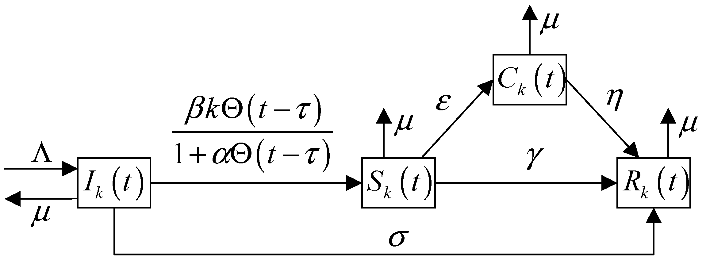
Figure 2.
The densities of .
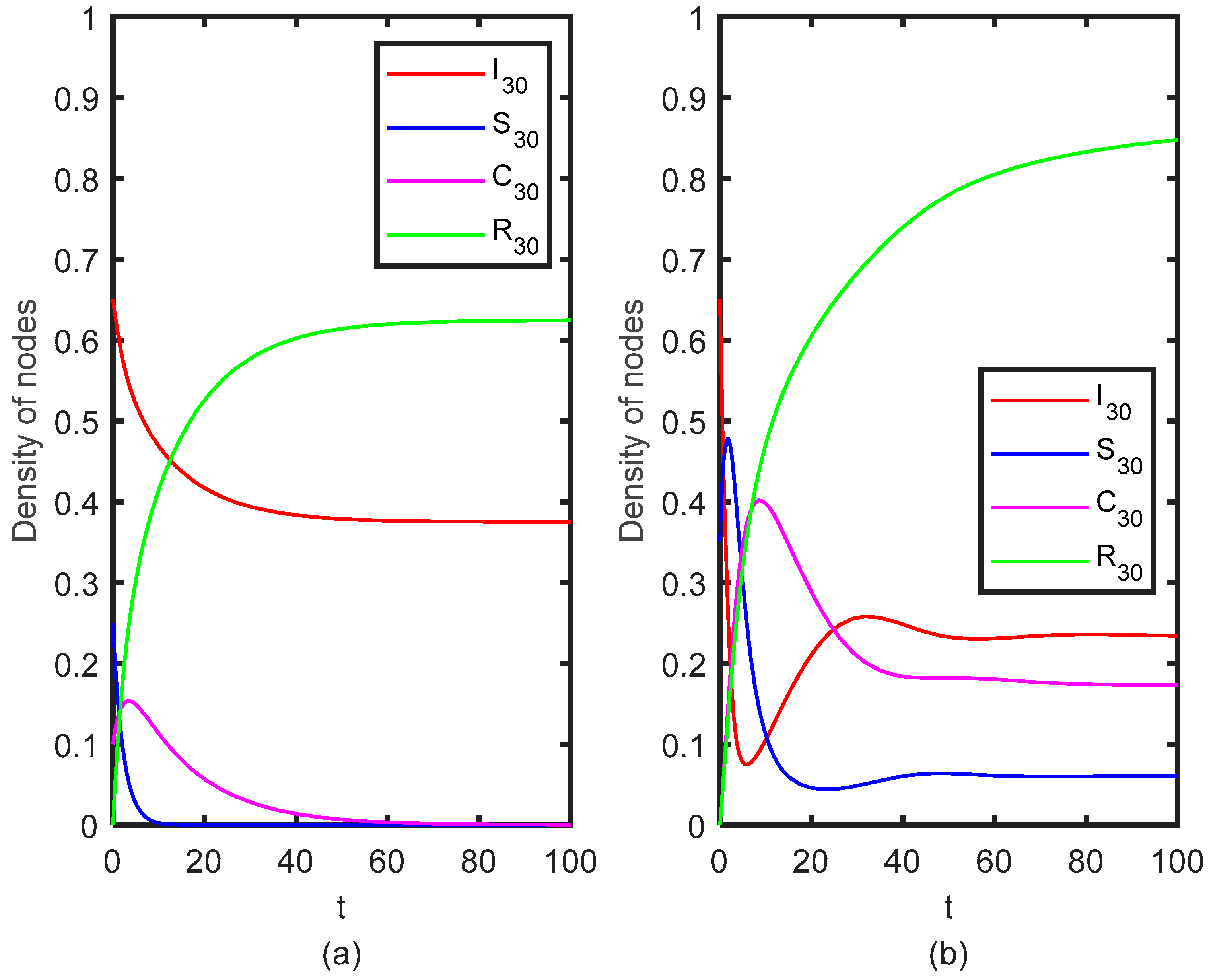
Figure 3.
The densities of , considering the variance of when .
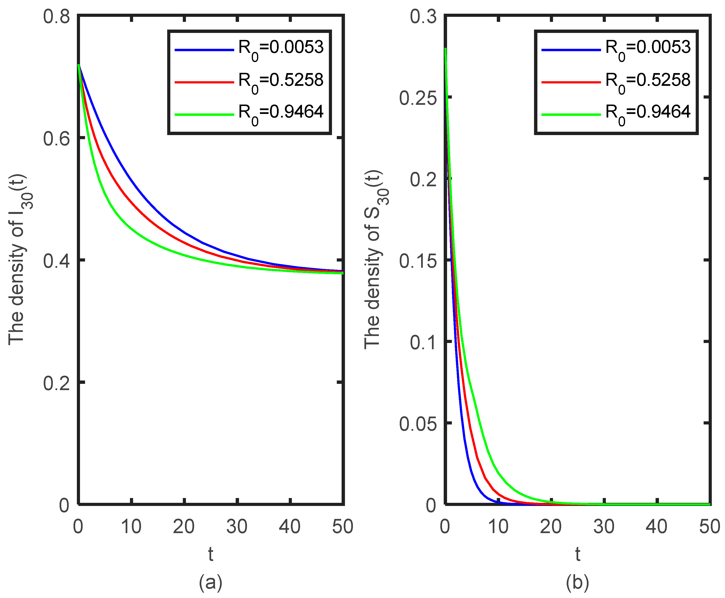
Figure 4.
The densities of , considering the variance of when .
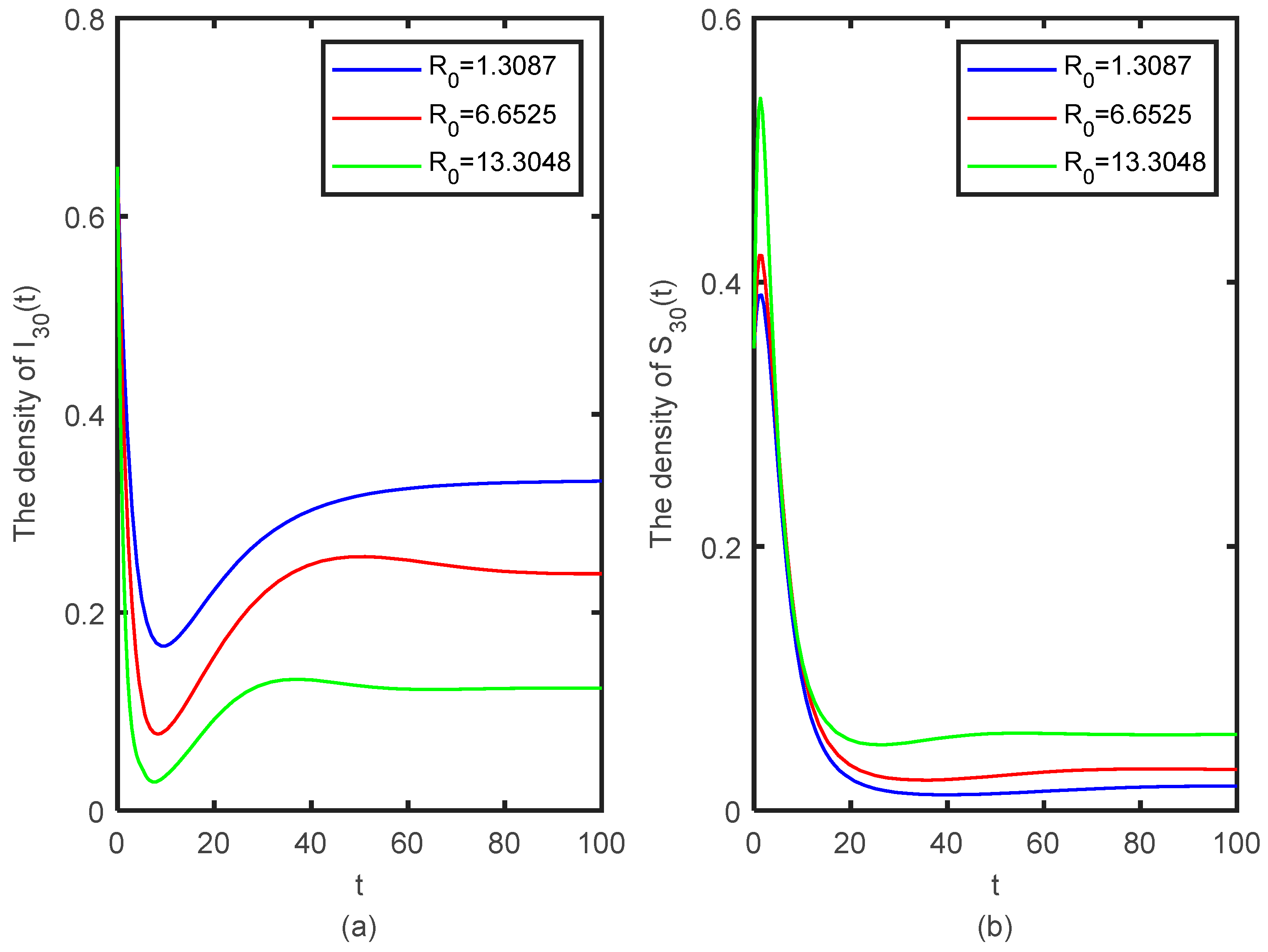
Figure 5.
The densities of (a) and ; (b), considering the different degrees of .

Figure 6.
The densities of (a) and ; (b) with different when .

Figure 7.
The densities of (a) and ; (b) for different time delays when .
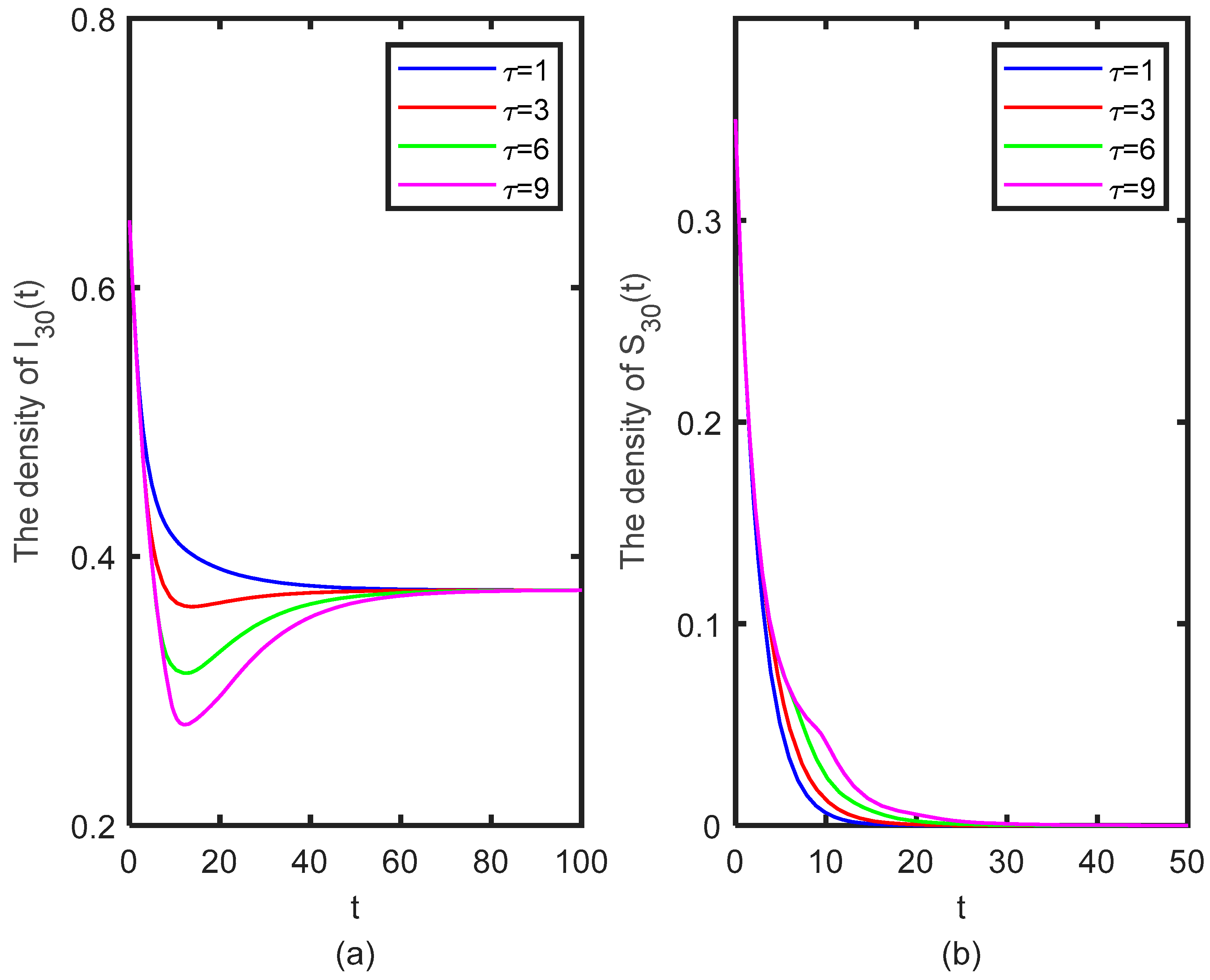
Figure 8.
The densities of (a) and ; (b) for different time delays when .
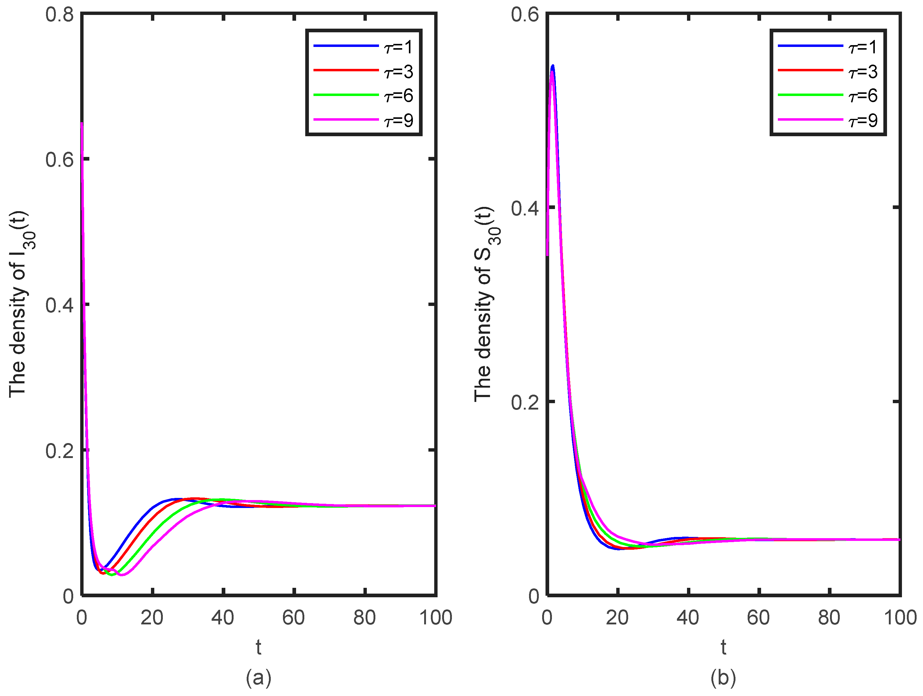
Figure 9.
The densities of with and without the optimal control.
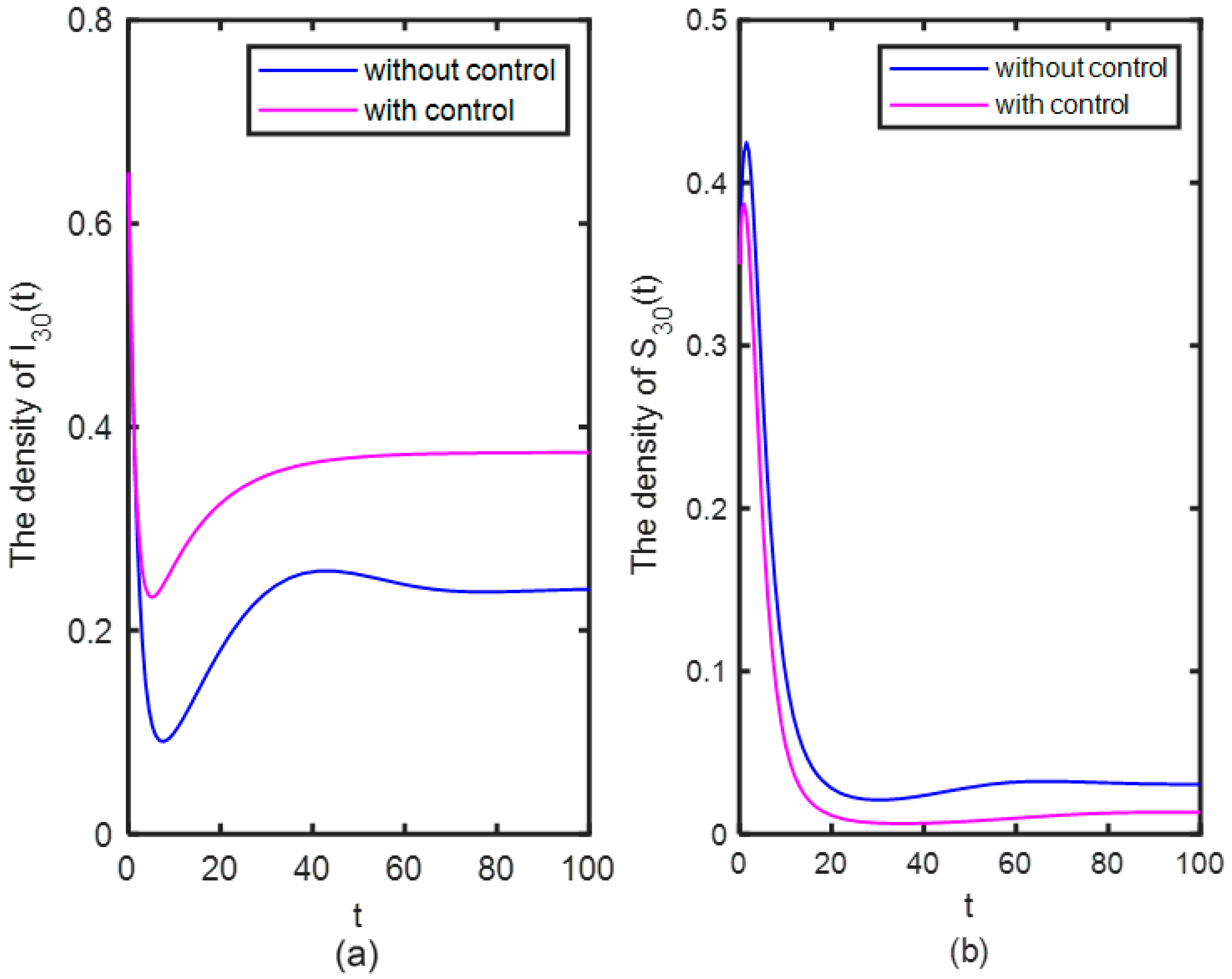
Figure 10.
The densities of with and without the Cooling-off state.

Publisher’s Note: MDPI stays neutral with regard to jurisdictional claims in published maps and institutional affiliations. |
© 2022 by the authors. Licensee MDPI, Basel, Switzerland. This article is an open access article distributed under the terms and conditions of the Creative Commons Attribution (CC BY) license (https://creativecommons.org/licenses/by/4.0/).
Share and Cite
MDPI and ACS Style
Yue, X.; Huo, L. Analysis of the Stability and Optimal Control Strategy for an ISCR Rumor Propagation Model with Saturated Incidence and Time Delay on a Scale-Free Network. Mathematics 2022, 10, 3900. https://doi.org/10.3390/math10203900
AMA Style
Yue X, Huo L. Analysis of the Stability and Optimal Control Strategy for an ISCR Rumor Propagation Model with Saturated Incidence and Time Delay on a Scale-Free Network. Mathematics. 2022; 10(20):3900. https://doi.org/10.3390/math10203900
Chicago/Turabian StyleYue, Xuefeng, and Liangan Huo. 2022. "Analysis of the Stability and Optimal Control Strategy for an ISCR Rumor Propagation Model with Saturated Incidence and Time Delay on a Scale-Free Network" Mathematics 10, no. 20: 3900. https://doi.org/10.3390/math10203900
Note that from the first issue of 2016, this journal uses article numbers instead of page numbers. See further details here.