
Modeling the Interplay between HDV and HBV in Chronic HDV/HBV Patients

 and
and 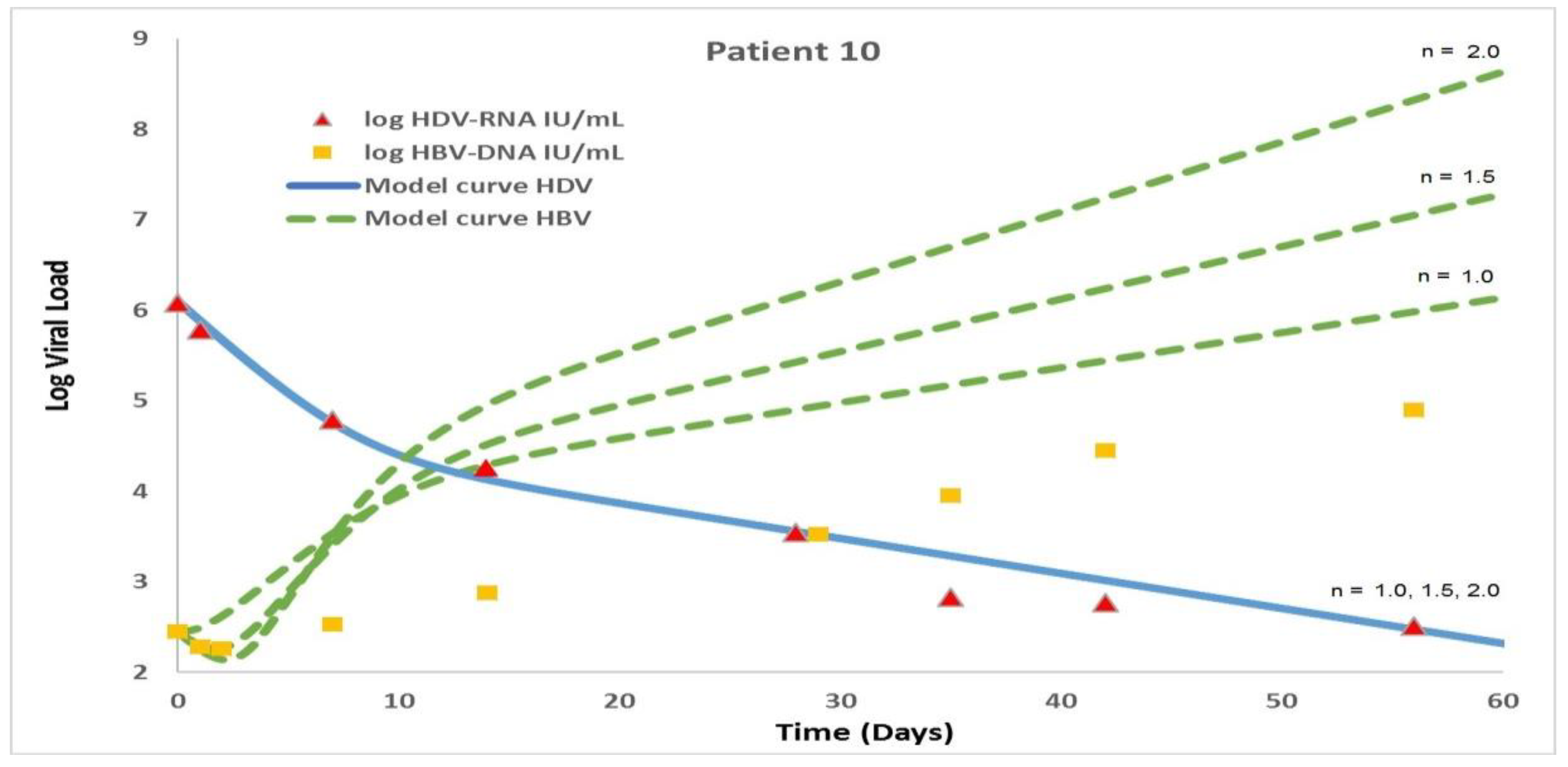
Abstract
:1. Introduction
2. Background
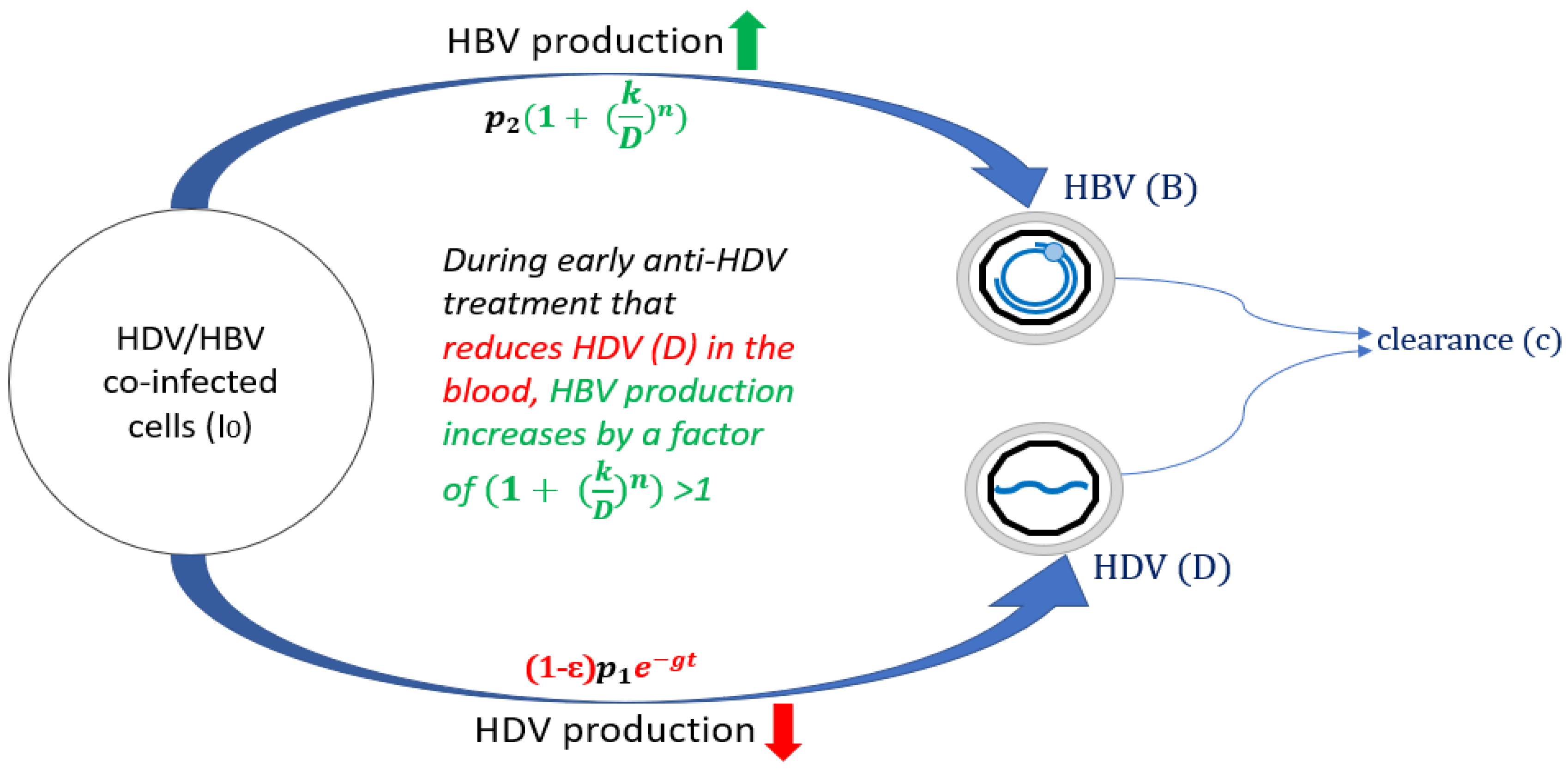
3. Modified Model
4. Results
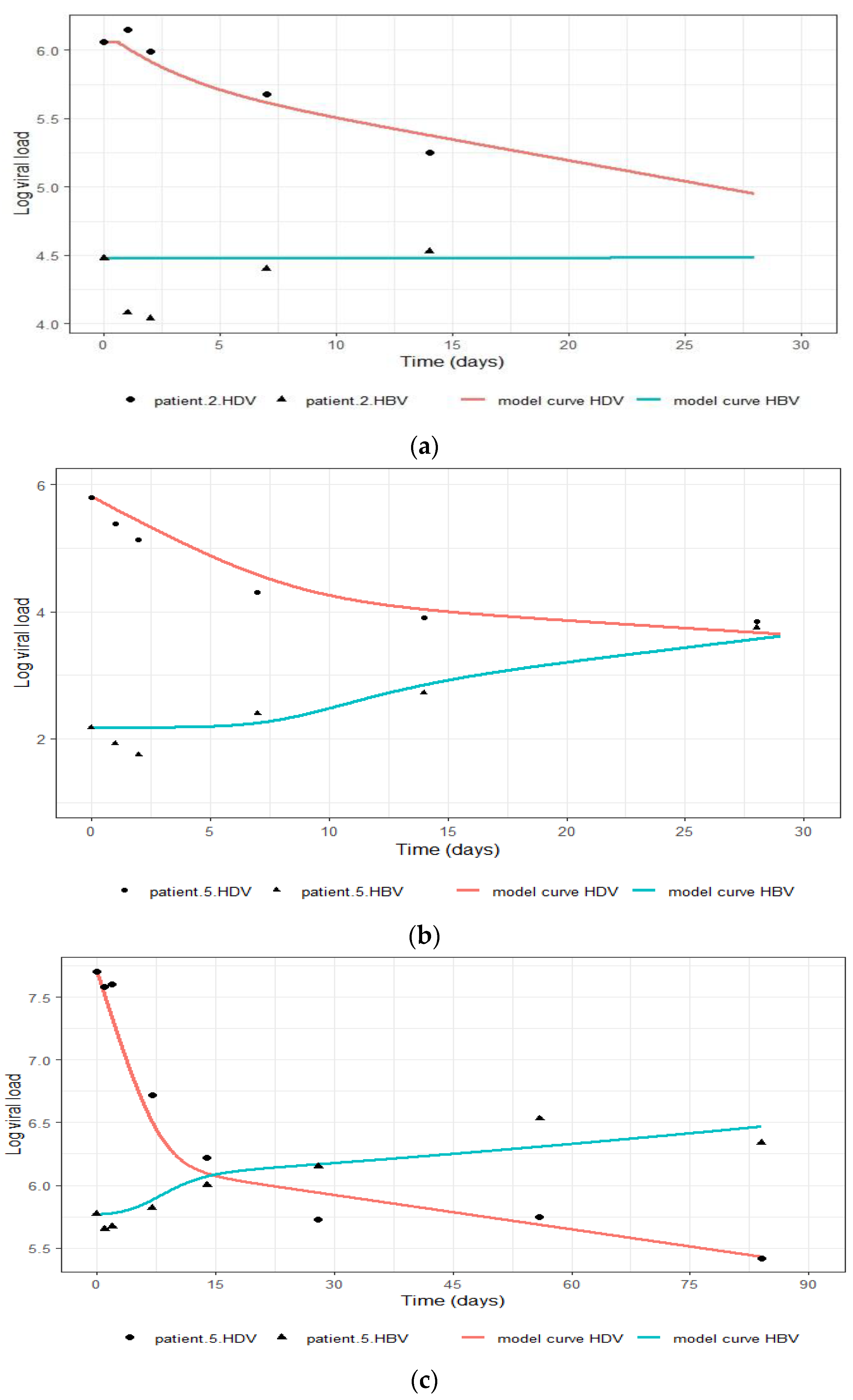
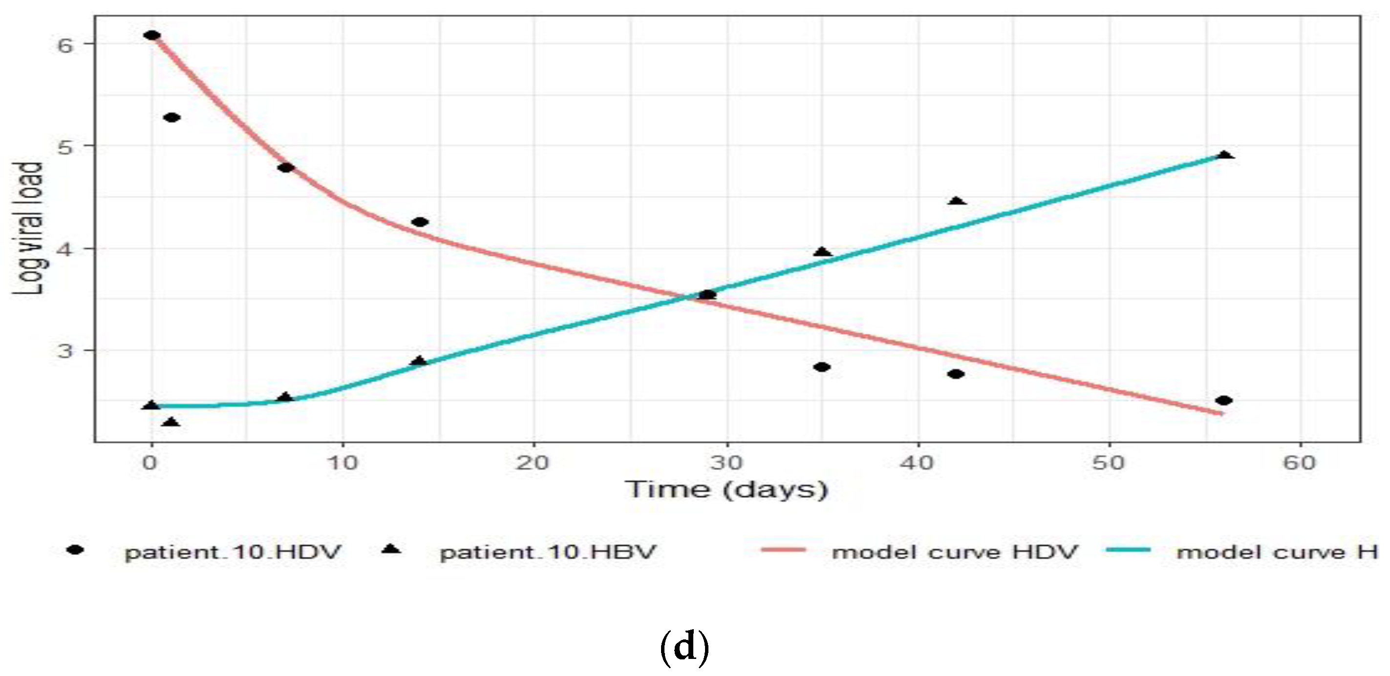
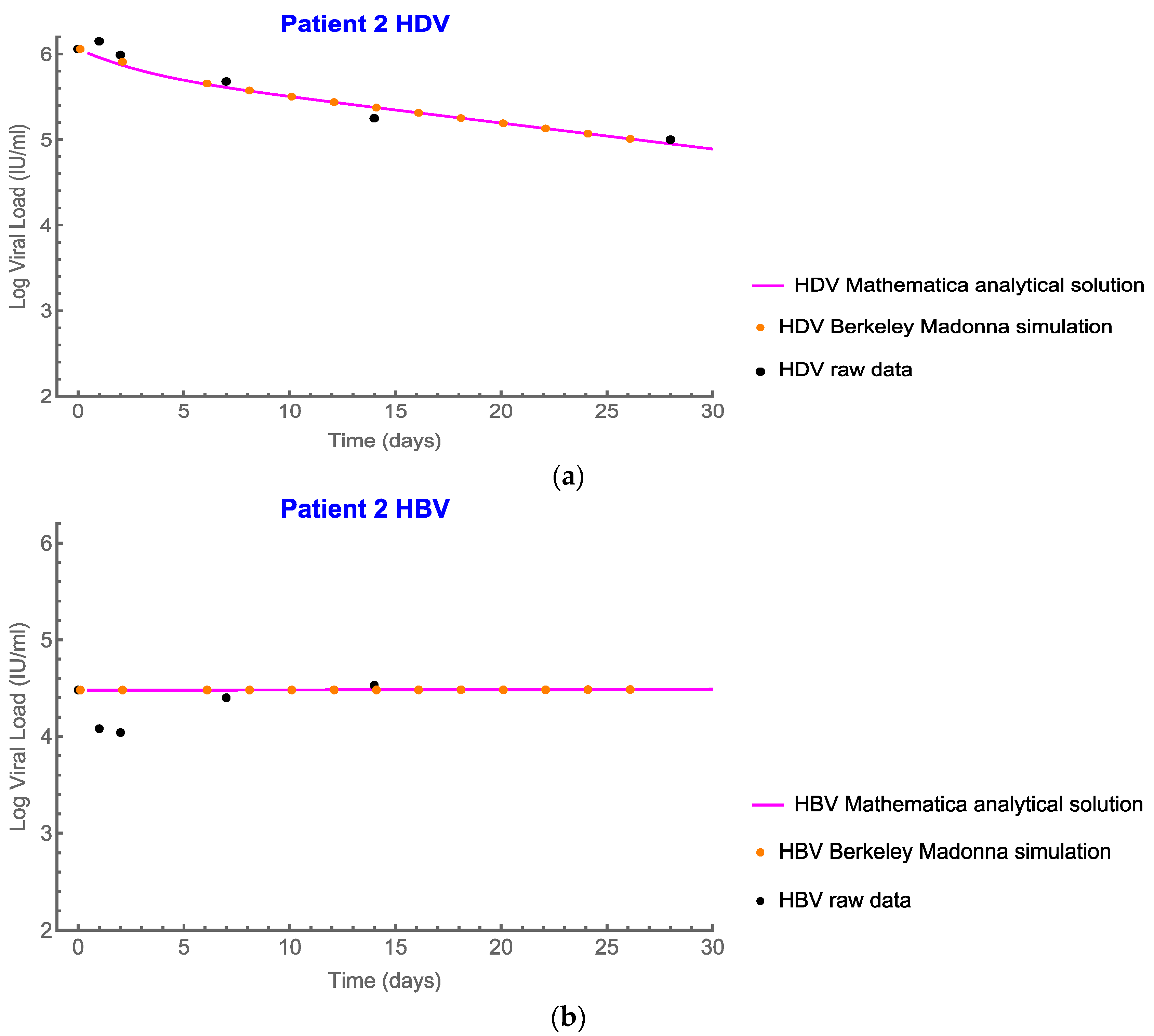
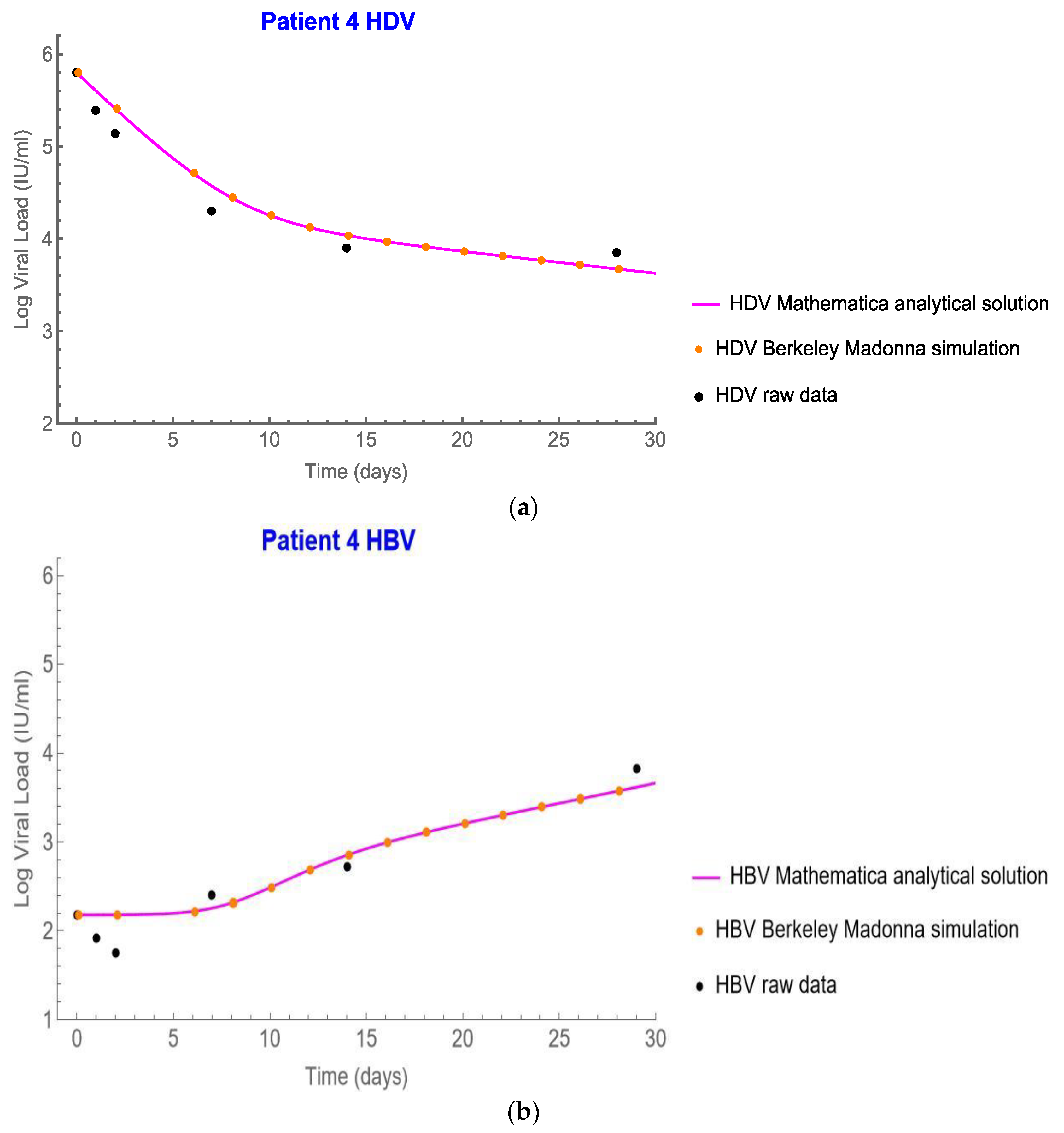
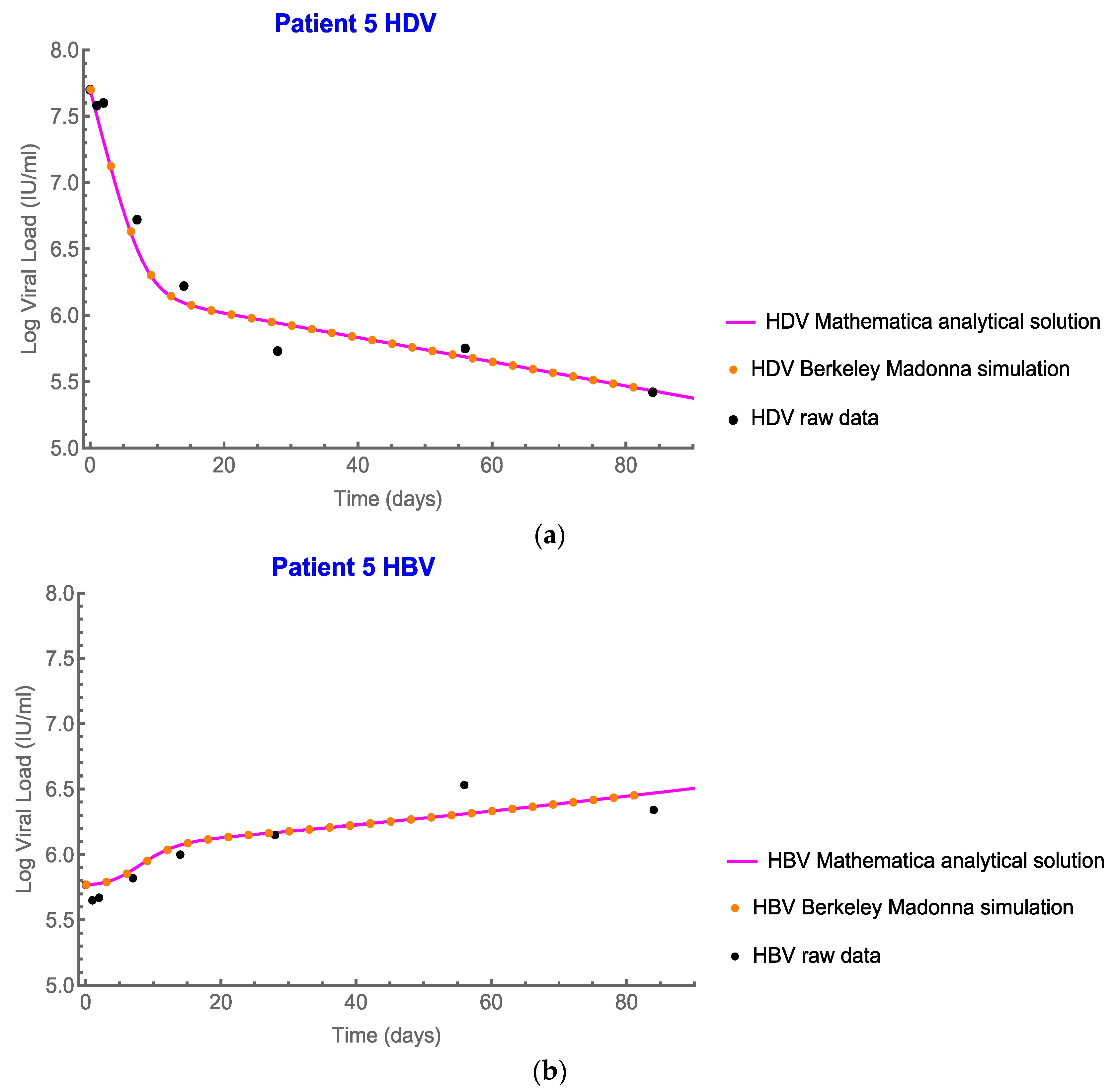
4.1. The Modified Model Simulates the Measured Data
4.2. Analytic Solutions
4.3. Analytic Solutions for HDV
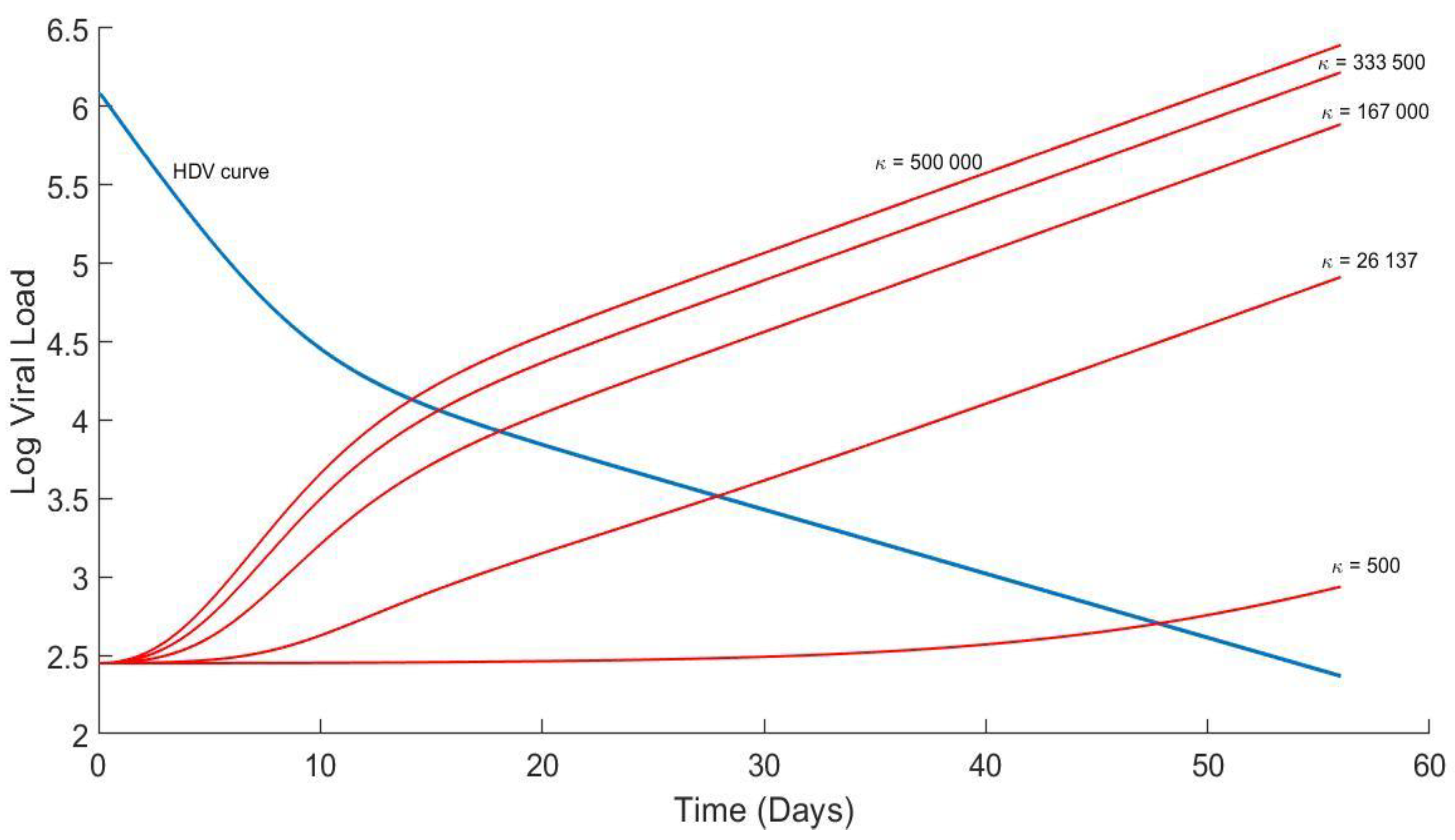
4.4. Analytical Solution for HBV and Plots
5. Discussion and Conclusions
Author Contributions
Funding
Institutional Review Board Statement
Data Availability Statement
Acknowledgments
Conflicts of Interest
Appendix A


References
- Stockdale, A.J.; Kreuels, B.; Henrion, M.Y.R.; Giorgi, E.; Kyomuhangi, I.; de Martel, C.; Hutin, Y.; Geretti, A.M. The global prevalence of hepatitis D virus infection: Systematic review and meta-analysis. J. Hepatol. 2020, 73, 523–532. [Google Scholar] [CrossRef] [PubMed]
- Miao, Z.; Zhang, S.; Ou, X.; Li, S.; Ma, Z.; Wang, W.; Peppelenbosch, M.P.; Liu, J.; Pan, Q. Estimating the Global Prevalence, Disease Progression, and Clinical Outcome of Hepatitis Delta Virus Infection. J. Infect. Dis. 2020, 221, 1677–1687. [Google Scholar] [CrossRef] [PubMed]
- Rizzetto, M.; Canese, M.G.; Arico, S.; Crivelli, O.; Trepo, C.; Bonino, F.; Verme, G. Immunofluorescence detection of new antigen-antibody system (delta/anti-delta) associated to hepatitis B virus in liver and in serum of HBsAg carriers. Gut 1977, 18, 997–1003. [Google Scholar] [CrossRef] [PubMed] [Green Version]
- Koh, C.; Heller, T.; Glenn, J.S. Pathogenesis of and New Therapies for Hepatitis D. Gastroenterology 2019, 156, 461–476.e1. [Google Scholar] [CrossRef] [PubMed]
- Engelke, M.; Mills, K.; Seitz, S.; Simon, P.; Gripon, P.; Schnolzer, M.; Urban, S. Characterization of a hepatitis B and hepatitis delta virus receptor binding site. Hepatology 2006, 43, 750–760. [Google Scholar] [CrossRef] [PubMed]
- Yardeni, D.; Heller, T.; Koh, C. Chronic hepatitis D-What is changing? J. Viral Hepat. 2022, 29, 240–251. [Google Scholar] [CrossRef] [PubMed]
- Heller, T.; Rotman, Y.; Koh, C.; Clark, S.; Haynes-Williams, V.; Chang, R.; McBurney, R.; Schmid, P.; Albrecht, J.; Kleiner, D.E.; et al. Long-term therapy of chronic delta hepatitis with peginterferon alfa. Aliment. Pharmacol. Ther. 2014, 40, 93–104. [Google Scholar] [CrossRef] [PubMed]
- Terrault, N.A.; Lok, A.S.F.; McMahon, B.J.; Chang, K.M.; Hwang, J.P.; Jonas, M.M.; Brown, R.S., Jr.; Bzowej, N.H.; Wong, J.B. Update on prevention, diagnosis, and treatment of chronic hepatitis B: AASLD 2018 hepatitis B guidance. Hepatology 2018, 67, 1560–1599. [Google Scholar] [CrossRef] [PubMed] [Green Version]
- European Association for the Study of the Liver. Electronic address eee, European Association for the Study of the L. EASL 2017 Clinical Practice Guidelines on the management of hepatitis B virus infection. J. Hepatol. 2017, 67, 370–398. [Google Scholar] [CrossRef] [PubMed] [Green Version]
- Guedj, J.; Rotman, Y.; Cotler, S.J.; Koh, C.; Schmid, P.; Albrecht, J.; Haynes-Williams, V.; Liang, T.J.; Hoofnagle, J.H.; Heller, T.; et al. Understanding early serum hepatitis D virus and hepatitis B surface antigen kinetics during pegylated interferon-alpha therapy via mathematical modeling. Hepatology 2014, 60, 1902–1910. [Google Scholar] [CrossRef]
- Zakh, R.; Churkin, A.; Bietsch, W.; Lachiany, M.; Cotler, S.J.; Ploss, A.; Dahari, H.; Barash, D. A Mathematical Model for early HBV and -HDV Kinetics during Anti-HDV Treatment. Mathematics 2021, 9, 3323. [Google Scholar] [CrossRef] [PubMed]
- Yurdaydin, C.; Keskin, O.; Kalkan, C.; Karakaya, F.; Caliskan, A.; Karatayli, E.; Karatayli, S.; Bozdayi, A.M.; Koh, C.; Heller, T.; et al. Optimizing lonafarnib treatment for the management of chronic delta hepatitis: The LOWR HDV-1 study. Hepatology 2018, 67, 1224–1236. [Google Scholar] [CrossRef] [PubMed] [Green Version]
- Olde, D.; Adri, B. NIST Handbook of Mathematical Functions; Cambridge University Press: Cambridge, UK, 2010. [Google Scholar]
- Shekhtman, L.; Cotler, S.J.; Hershkovich, L.; Uprichard, S.L.; Bazinet, M.; Pantea, V.; Cebotarescu, V.; Cojuhari, L.; Jimbei, P.; Krawczyk, A.; et al. Modelling hepatitis D virus RNA and HBsAg dynamics during nucleic acid polymer monotherapy suggest rapid turnover of HBsAg. Sci. Rep. 2020, 10, 7837. [Google Scholar] [CrossRef]
- Koh, C.; Canini, L.; Dahari, H.; Zhao, X.; Uprichard, S.L.; Haynes-Williams, V.; Winters, M.A.; Subramanya, G.; Cooper, S.L.; Pinto, P.; et al. Oral prenylation inhibition with lonafarnib in chronic hepatitis D infection: A proof-of-concept randomised, double-blind, placebo-controlled phase 2A trial. Lancet Infect. Dis. 2015, 15, 1167–1174. [Google Scholar] [CrossRef] [Green Version]
- Kadelka, S.; Dahari, H.; Ciupe, S.M. Understanding the antiviral effects of RNAi-based therapy in HBeAg-positive chronic hepatitis B infection. Sci. Rep. 2021, 11, 200. [Google Scholar] [CrossRef] [PubMed]
- Reinharz, V.; Ishida, Y.; Tsuge, M.; Durso-Cain, K.; Chung, T.L.; Tateno, C.; Perelson, A.S.; Uprichard, S.L.; Chayama, K.; Dahari, H. Understanding Hepatitis B Virus Dynamics and the Antiviral Effect of Interferon Alpha Treatment in Humanized Chimeric Mice. J. Virol. 2021, 95, e0049220. [Google Scholar] [CrossRef] [PubMed]
- Shirvani-Dastgerdi, E.; Tacke, F. Molecular interactions between hepatitis B virus and delta virus. World J. Virol. 2015, 4, 36–41. [Google Scholar] [CrossRef] [PubMed]
- De Sousa, B.C.; Cunha, C. Development of mathematical models for the analysis of hepatitis delta virus viral dynamics. PLoS ONE 2010, 5, e12512. [Google Scholar] [CrossRef] [PubMed] [Green Version]
- Packer, A.; Forde, J.; Hews, S.; Kuang, Y. Mathematical models of the interrelated dynamics of hepatitis D and B. Math. Biosci. 2014, 247, 38–46. [Google Scholar] [CrossRef]
- Goyal, A.; Murray, J.M. Dynamics of in vivo hepatitis D virus infection. J. Theor. Biol. 2016, 398, 9–19. [Google Scholar] [CrossRef] [PubMed]


Publisher’s Note: MDPI stays neutral with regard to jurisdictional claims in published maps and institutional affiliations. |
© 2022 by the authors. Licensee MDPI, Basel, Switzerland. This article is an open access article distributed under the terms and conditions of the Creative Commons Attribution (CC BY) license (https://creativecommons.org/licenses/by/4.0/).
Share and Cite
Mhlanga, A.; Zakh, R.; Churkin, A.; Reinharz, V.; Glenn, J.S.; Etzion, O.; Cotler, S.J.; Yurdaydin, C.; Barash, D.; Dahari, H. Modeling the Interplay between HDV and HBV in Chronic HDV/HBV Patients. Mathematics 2022, 10, 3917. https://doi.org/10.3390/math10203917
Mhlanga A, Zakh R, Churkin A, Reinharz V, Glenn JS, Etzion O, Cotler SJ, Yurdaydin C, Barash D, Dahari H. Modeling the Interplay between HDV and HBV in Chronic HDV/HBV Patients. Mathematics. 2022; 10(20):3917. https://doi.org/10.3390/math10203917
Chicago/Turabian StyleMhlanga, Adequate, Rami Zakh, Alexander Churkin, Vladimir Reinharz, Jeffrey S. Glenn, Ohad Etzion, Scott J. Cotler, Cihan Yurdaydin, Danny Barash, and Harel Dahari. 2022. "Modeling the Interplay between HDV and HBV in Chronic HDV/HBV Patients" Mathematics 10, no. 20: 3917. https://doi.org/10.3390/math10203917