Article

Functional Ergodic Time Series Analysis Using Expectile Regression

by
Fatimah Alshahrani
1,
Ibrahim M. Almanjahie
2,3,
Zouaoui Chikr Elmezouar
2,*,
Zoulikha Kaid
2,
Ali Laksaci
2 and
Mustapha Rachdi
4
1
Department of Mathematical Sciences, College of Science, Princess Nourah bint Abdulrahman University, Riyadh 11671, Saudi Arabia
2
Department of Mathematics, College of Science, King Khalid University, Abha 62529, Saudi Arabia
3
Statistical Research and Studies Support Unit, King Khalid University, Abha 62529, Saudi Arabia
4
Laboratory AGEIS, University of Grenoble Alpes (France), EA 7407, AGIM Team, UFR SHS, BP. 47, CEDEX 09, F38040 Grenoble, France
*
Author to whom correspondence should be addressed.
Mathematics 2022, 10(20), 3919; https://doi.org/10.3390/math10203919
Submission received: 22 September 2022 / Revised: 18 October 2022 / Accepted: 19 October 2022 / Published: 21 October 2022

Abstract

:
In this article, we study the problem of the recursive estimator of the expectile regression of a scalar variable Y given a random variable X that belongs in functional space. We construct a new estimator and study the asymptotic properties over a general functional time structure. Precisely, the strong consistency of this estimator is established, considering that the sampled observations are taken from an ergodic functional process. Next, a simulation experiment is conducted to highlight the great impact of the constructed estimator as well as the ergodic functional time series data. Finally, a real data analysis is used to demonstrate the superiority of the constructed estimator.

1. Introduction

Consider the sequence ( X i , Y i ) i = 1 , , n of dependent random variables that have taken values in F × I R . The F is assumed to be a semi-metric space that has a semi-metric d (.,.) and ( X i , Y i ) i = 1 , , n is strictly stationary. Let E p ( x ) be the p-conditional expectile, and for x F and p ( 0 , 1 ) , the E p ( x ) is
E p ( x ) = arg min t I E p 1 I Y t > 0 ( Y t ) 2 X = x .
The 1 I Y t > 0 is an indicator function and we use the set A to refer to it as 1 I A .
Assuming that the observations are strictly stationary ergodic data and based on a recursive kernel method, we deal, in this study, with the nonparametric estimation problem in the case of the expectile regression. Comparing the recursive method to the classical kernel estimation, the first is more informative and has a substantial advantage, which is the possibility of updating estimates for each additional piece of information. Such a feature is crucial in financial time series data. Indeed, the observations are obtainable through real-time monitoring, and each new piece of information has a great impact on risk analysis. Thus, a real-time update of the estimation of the expectile model as a risk tool is crucial. The classical estimator fails to do this since it does not allow the renewal of the estimator for each additional piece of information. Therefore, the recursive estimation of the expectile regression is more relevant in financial time series. From a bibliographical point of view, the recursive estimation in the functional area was introduced by Amiri et al. [1], who studied the recursive estimation of the regression operator. The recursive smoothing method has been employed for the conditional mode, as an alternative functional conditional model, by Ardjoun et al. [2] and the quantile regression by Benziadi et al. [3]. More recent advances and references in functional nonparametric estimation by recursive techniques can be found in Slaoui [4,5] or Laksaci et al. [6]. In parallel, the ergodic functional time series data were started by Laib and Louani [7,8], who proved the complete consistency together with the normality asymptotic of the kernel estimator of the conditional expectation. The robust regression was studied by Gheriballah et al. [9], who expressed the consistency of the kernel estimator of the M-regression. We focus, in this study, on a new regression model, the so-called expectile regression. The latter has a great impact on the financial time series. In particular, it is usually used as a risk measure in finance and actuarial science. For a good description of the background of this model and its applications, we refer readers to Pratesi et al. [10], Waltrup et al. [11] or Farooq and Steinwart [12] and Daouia and Paindaveine [13]. While all these works treat the case when the regressor is of finite dimension and parametric case, our contribution focuses in the general case. Since the regressors are not necessary for finite dimensions, the model’s observations are not necessarily independent, and the model is not necessarily linear. Indeed, the literature is still limited to the nonparametric estimation method in the case of expectile regression. In particular, the initial results were determined by Mohammedi et al. [14], who derived the complete consistency of the kernel estimator of the conditional expectile and the asymptotic normality. We refer to Almanjahie et al. [15] for the uniform consistency of the kNN estimator of this model. While all the previous results were stated in the independence case, we treat the dependence case in this paper. Our primary aim is to investigate the complete convergence (see Ferraty and Vieu [16]) of a functional recursive kernel estimate of E p ( x ) using the structure of ergodicity. It is worth noting that adapting the recursive estimation approach in the case of ergodic functional time series is very much desirable. Firstly, it is well known that, in time series analysis, the recursive estimation approach is more relevant than the standard kernel approach (see Roussas and Tran [17]). Moreover, the recursive estimator can be viewed as a generalization of the classical kernel approach. On the other hand, the ergodicity hypothesis, considered here, is an alternative dependence condition for the strong mixing conditions studied by Almanjahie et al. [18]. Furthermore, the ergodicity is simpler than the strong mixing condition since the latter is very hard to check in practice. It should be noted that the ergodicity structure and the expectile regression are beneficial in financial areas. In particular, the expectile regression is a good risk detector, and functional ergodicity is the natural correlation structure of financial time series data. Indeed, the financial data is usually modeled as a GARCH process for which its mixing property is not trivial. Finally, let us point out that even if the “expectile regression" and “recursive estimation" are not well known in nonparametric statistics, their combination together allows to accumulate advantages of both approaches in order to increase the reliability of the studied nonparametric model as a powerful instrument in risk management. In particular, it permits profiting from real-time updating or the online feature of the recursive algorithm to identify the financial risk instantly. The reader interested in the merits of the recursive estimation may refer to Wolverton and Wagner [19] and Yamato [20] as precursor works or Bouzebda and Slaoui [21] or Slaoui [22] for recent advances and references. For more discussion on the importance of the expectile function and its feasibility in practice we cite Jones [23], Abdous and Rémillard [24], Bellini et al. [25] and Girard et al. [26] for recent developments and applications.
The paper outline is as follows. The general framework is introduced in Section 2. Section 3 presents the asymptotic properties of the constructed recursive kernel estimator. Some special cases are discussed in Section 4. Section 5 is devoted to computational study and real data over artificial data. The conclusion is stated in Section 6. Finally, an appendix is provided detailing the auxiliary results’ proofs.

2. Methodology

2.1. The Ergodic Functional Data Framework

As pointed out before, the general framework of this contribution is the functional ergodic time series analysis as a natural area of financial time series data. Note that the dependence setting is an alternative structure to the strong mixing process, often considered in functional time series analysis. However, it is well known that handling the condition of the ergodicity is more manageable than the mixing condition since the latter requires calculating the supremum over two infinite σ -algebras. Moreover, the ergodicity condition is less restrictive compared to the mixing assumption. Recall that, in classical statistics, the ergodicity condition is defined concerning an ergodic transformation. In the context of functional statistics, we follow Laib and Louani [7]) and consider their introduced definition. Furthermore, the functional ergodic time series analysis also uses the concentration property of the functional co-variate over the small ball defined, for r > 0 , by B ( x , r ) = x F / d ( x , x ) < r . In particular, the concentration property in this dependence setting should take into account the ergodicity assumption. Specifically, our functional ergodic framework is carried out by the assumptions stated below.
Suppose the σ -fields F k and G k , where k = 1 , , n are generated, respectively, by ( ( X 1 , Y 1 ) , ( X k , Y k ) ) and ( ( X 1 , Y 1 ) , ( X k , Y k ) , ( X k + 1 , Y k + 1 ) . Then, the strictly stationary ergodic process ( X i , Y i ) i I N satisfies:
(H1) 
( i )   T h e   f u n c t i o n   ϕ x ( r ) = I P ( X B ( x , r ) ) i s   s u c h   t h a t   ϕ x ( r ) > 0 , r > 0 a n d   s [ 0 , 1 ] , lim r 0 ϕ x ( s r ) / ϕ x ( r ) = τ x ( s ) < . ( i i )   T h e r e   e x i s t s   a   n o n n e g a t i v e   r a n d o m   s e q u e n c e   ( C i ) i   s u c h   t h a t r > 0 I P X i B ( x , r ) | F i 1 = C i ϕ x ( r ) + o ( ϕ x ( r ) ) , ( i i i )   F o r   a l l m 2 , 1 n ϕ x m ( h n ) i = 1 n C i ϕ x m ( h i ) C m , x > 0 , a.co.
We note that this consideration is more general concerning the ergodicity framework considered by Laib and Louani [7] in the sense that in the present work, it is not required to assume that the concentration I P X i B ( x , r ) or I P X i B ( x , r ) | F i 1 as a product resulted in the contribution of two independent positive functions (in x and r). This gain is very important because it avoids assuming the existence of the Onsager–Machlup function, which requires additional assumptions (see Bogachev [27]).

2.2. Model and Estimator

This section details the constructed recursive estimator of the expectile regression E p ( x ) defined by (1). It is important to note that the loss function in (1) generalizes the least square function of E ( Y X = x ). It coincides with this function once p = 0.5 . In spite of that, the score function of (1) is also similar to the conditional pth-quantile of Y given X = x . Indeed, the difference in the absolute value | Y t | is replaced by ( Y t ) 2 . Moreover, similarly to the e regression by quantile, the expectile regression can be explicitly expressed using some analytical arguments. Precisely, the E p ( x ) is the solution w.r.t. t of
p 1 p = G ( t ; x ) : = G 1 ( t ; x ) G 2 ( t ; x ) ,
with
G 1 ( t ; x ) = I E ( Y t ) 1 I ( Y t ) 0 X = x , G 2 ( t ; x ) = I E ( Y t ) 1 I ( Y t ) > 0 X = x .
Hence, we use the monotony of G ( · ; x ) to conclude that
E p ( x ) = inf t I R : G ( t ; x ) p 1 p .
The recursive kernel estimator of the function G ( · ; x ) is defined via an index l [ 0 , 1 ] by
G ^ ( n , l , t ; x ) = i = 1 n W n i ( x ) ( Y i t ) 1 I ( Y i t ) 0 i = 1 n W n i ( x ) ( Y i t ) 1 I ( Y i t ) > 0 , for t I R ,
where
W n i ( x ) = ϕ x l ( h i ) K ( h i 1 d ( x , X i ) ) i = 1 n ϕ x l ( h i ) K ( h i 1 d ( x , X i ) ) .
K indicates a kernel and ( a n ) n refers to a sequence of positive real numbers in which lim n a n = 0 . Hence, the recursive kernel estimator of E p ( x ) denoted by E ^ p ( x ) is explicitly obtained with
E ^ p ( x ) = inf t I R : G ^ h ( l , t ; x ) p 1 p .
Observe that the recursive link between different steps of the estimator E ^ p ( x ) is obtained through the recursive property of G ^ ( n , l , t ; x ) , for which we can write
G ^ ( n + 1 , l , t ; x ) = i = 1 n ϕ x 1 l ( h i ) G ^ 1 ( l , t ; x ) + i = 1 n ϕ x 1 l ( h i ) Y i t ) 1 I ( Y i t ) 0 K ^ ( n + 1 , l , t ; x ) i = 1 n ϕ x 1 l ( h i ) G ^ 2 ( l , t ; x ) + i = 1 n ϕ x 1 l ( h i ) ( Y i t ) 1 I ( Y i t ) > 0 K ^ ( n + 1 , l , t ; x )
where
G ^ 1 ( l , t ; x ) = 1 i = 1 n ϕ x 1 l ( h i ) i = 1 n W n i ( x ) ( Y i t ) 1 I ( Y i t ) 0 ,
G ^ 2 ( l , t ; x ) = 1 i = 1 n ϕ x 1 l ( h i ) i = 1 n W n i ( x ) ( Y i t ) 1 I ( Y i t ) > 0
and
K ^ ( i , l , t ; x ) = 1 ϕ x ( h i ) j = 1 i ϕ x 1 l ( h i ) K ( h i 1 d ( x , X i ) )

3. Main Results

To analyze the asymptotic behaviour of the constructed estimator, E p ^ ( x ) , the following conditions are required. In what follows, we use C or C to represent some strictly positive constants.
(A1) 
G ( · ; x ) is differentiable in R and it satisfies: a > 0 , t E p ( x ) a , E p ( x ) + a , x 1 , x 2 F ,
| G i ( t ; x 1 ) G i ( t ; x 2 ) | C d β i ( x 1 , x 2 ) , for β i > 0 , i { 1 , 2 } .
(A2) 
For q 2 φ q ( Y ) = I E | Y | q X C < , a.s. ,
(A3) 
The kernel K is supported within ( 0,1 ) and has a continuous derivative on ( 0,1 ) , such that
0 < C 1 I ( 0,1 ) ( · ) K ( · ) C 1 I ( 0,1 ) ( · ) and K ( 1 ) 0 1 K ( s ) τ x ( s ) d s > 0 .
(A4) 
The sequence of the bandwidth parameter ( h i ) i = 1 , n such that
( i )   For   all   m 2 , 1 n ϕ x m ( h n ) i = 1 n ϕ x m ( h i ) C m > 0 , a.co. ( ii )   For   l 1   and   a > q + 1     we   have , n 2 a / q 1 ϕ x 2 l 1 ( h n ) ϕ x 2 l ( h n ) log n 0 with   h n = min i = 1 , n ( h i ) .
Clearly, condition (A4) is closely linked to our functional ergodic framework, which is illustrated by condition (H1). It is also linked to the recursivity of the estimator. Nevertheless, condition (A4) can be considered as a technical assumption allowing to simplify the technical results.
Theorem 1.
If conditions (A1)–(A4) are fulfilled and suppose that G ( t ; x ) t | t = E p ( x ) > 0 ; then, we have, as n ,
E p ^ h ( x ) E p ( x ) = O a.co. h n min ( β 1 , β 2 ) + log n n ϕ x ( h n ) .
Proof of the Theorem 1.
For some ϵ 0 > 0 , we introduce
z n = ϵ 0 h n min ( β 1 , β 2 ) + log n n ϕ x ( h n ) .
We can see that
n I P | E p ^ ( x ) E p ( x ) | > z n n I P sup t [ E p ( x ) δ , E p ( x ) + δ ] | G ^ ( n , l , t ; x ) G ( t ; x ) | C z n < .
Therefore, Theorem 1 is a result of the below statement:
sup t [ E p ( x ) δ , E p ( x ) + δ ] G ^ ( n , l , t ; x ) G ( t ; x ) = O a.co. z n .
We start by writing
G ^ ( n , l , t ; x ) G ( t ; x ) = B ^ n ( l , t ; x ) + R ^ n ( l , t ; x ) G ^ D ( l , t ; x ) + Q ^ n ( l , t ; x ) G ^ D ( l , t ; x )
where
Q ^ n ( l , t ; x ) : = ( G ^ N ( l , t ; x ) G ¯ N ( l , t ; x ) ) G ( t ; x ) ( G ^ D ( l , t ; x ) G ¯ D ( l , t ; x ) ) , B ^ n ( l , t ; x )     : = G ¯ N ( l , t ; x ) G ¯ D ( l , t ; x ) G ( t ; x ) and R ^ n ( l , t ; x ) : = B ^ n ( l , t ; x ) ( G ^ D ( l , t ; x ) G ¯ D ( l , t ; x ) )
with
G ^ N ( l , t ; x ) : = 1 i = 1 n ϕ x 1 l ( h i ) i = 1 n ϕ x l ( h i ) K ( h i 1 d ( x , X i ) ) ( Y i t ) 1 I ( Y i t ) 0 , G ¯ N ( l , t ; x ) : = 1 i = 1 n ϕ x 1 l ( h i ) i = 1 n ϕ x l ( h i ) I E K ( h i 1 d ( x , X i ) ) ( Y i t ) 1 I ( Y i t ) 0 | G i 1 , G ^ D ( l , t ; x ) : = 1 i = 1 n ϕ x 1 l ( h i ) i = 1 n ϕ x l ( h i ) K ( h i 1 d ( x , X i ) ) ( Y i t ) 1 I ( Y i t ) > 0 , G ¯ D ( l , t ; x ) : = 1 i = 1 n ϕ x 1 l ( h i ) i = 1 n ϕ x l ( h i ) I E K ( h i 1 d ( x , X i ) ) ( Y i t ) 1 I ( Y i t ) > 0 | G i 1 .
Thus, Theorem 1 is a consequence of the following lemmas, where their proofs appear in Appendix A. □
Lemma 1.
Considering conditions (A1)–(A4), we obtain
sup t [ E p ( x ) δ , E p ( x ) + δ ] G ^ D ( l , t ; x ) G ¯ D ( l , t : x ) = O a.co. log n n ϕ x ( h n )
and
sup t [ E p ( x ) δ , E p ( x ) + δ ] G ^ N ( l , t ; x ) G ¯ N ( l , t ; x ) = O a.co. log n n ϕ x ( h n ) .
Lemma 2.
Using conditions of Lemma 1, we obtain
C > 0 n = 1 I P sup t [ E p ( x ) δ , E p ( x ) + δ ] G ^ D ( l , t ; x ) C < .
Lemma 3.
Considering conditions (A1)–(A3), we obtain
sup t [ E p ( x ) δ , E p ( x ) + δ ] | B ^ n ( l , t ; x ) | = O a.co. h n min ( β 1 , β 2 ) .

4. Some Special Cases

This study covers various general cases of functional statistics, and the obtained convergence rate expression is identifiable from the previous studies. Thus, to highlight this issue, the complete convergence rate is determined in the following special cases.
  • The classical kernel case: Evidently, this case can be viewed as a special case of our proposed method once h i = h n , for all 1 i n . Hence, condition (A4(ii)) is automatically fulfilled and (H1(iii)) and (A4(ii)) are replaced by
    1 n i = 1 n C i C and n 2 a / q 1 ϕ x ( h n ) log n 0 .
    where the following corollary gives the convergence rate.
    Corollary 1.
    Considering conditions (A1)–(A3) and (6), we obtain
    E p ˜ ( x ) E p ( x ) = O a.co. h n min ( β 1 , β 2 ) + log n n ϕ x ( h n ) .
    Remark 1.
    As far as we know, this result is also new in the field of nonparametric functional data analysis. In other words, no work in the literature considers conditional expectile estimation in the case of functional ergodic data.
  • Independence case: When the independent situation is considered, the (H1) condition can be reduced to the (H1(i)) condition. Therefore, Theorem 1 leads to the following corollary.
    Corollary 2.
    Considering conditions (A1)–(A4), we obtain
    E p ^ ( x ) E p ( x ) = O a.co. h n min ( β 1 , β 2 ) + log n n ϕ x ( h n ) .
    Remark 2.
    Once again, the above corollary is unique in the field of nonparametric functional data analysis. Indeed, the recursive estimate of functional expectile regression data has not been addressed previously in functional statistics.
  • The classical regression case: It should be clear to readers that classical regression is regarded as a special case of the expectile regression. It can be obtained easily by putting p = 0.5 . So, by simple calculation, we prove that
    E 0.5 ( x ) : = I E [ Y X = x ] and E 0.5 ^ ( x ) : = i = 1 n W n i ( x ) Y i .
    For this functional model, the condition (A2) is reformulated as
    x 1 , x 2 F , E 0.5 ( x 1 ) E 0.5 ( x 2 ) C 1 d a 1 ( x 1 , x 2 ) .
    Theorem 1 is now presented as follows.
    Corollary 3.
    Consider conditions (A1), (A3), (A4) and if (7) holds, then, as n , we obtain
    E 0.5 ^ ( x ) E 0.5 ( x ) = O a.co. h n min ( β 1 , β 2 ) + log n n ϕ x ( h n ) .
    Remark 3.
    Note that Amiri et al. [1] studied the function version of the recursive estimation method of the conditional expectation. However, they only stated the consistency of the estimator in the i.i.d. case. The novelty of the present paper is the treatment of the functional ergodic case. Thus, we can say that the result of corollary 3 is new in the context of nonparametric functional data analysis.

5. A Simulation Study

Our primary aim here is to evaluate the performance of the finite sample of the constructed estimator. Specifically, our primary purpose is to quantify the impact of the recursivity on the estimator’s efficiency. Of course, we evaluate this aspect on the precision, robustness and on-time execution of the estimator. To do that, we generate data from the functional GARCH model. Noting that the GARCH model is a popular structure for fitting the financial time series data (see, for instance, Feng et al. [28] or So et al. [29]). Furthermore, the ergodicity assumption of the GARCH model is easier than the mixing property. Thus, simulating by functional GARCH model permits the exploration of both axes of this work: ergodicity and recursivity. Typically, we obtain an artificial financial real-time series by considering a functional X ( t ) drown by the code-routine garchSim where the coefficients of the conditional variance are α = ( 0.1 t 2 , 0.2 t 2 ) and β = ( 0.05 t , 0.01 t ) . The functional X is discretized in the same grid of t formed by 100 points in [ 0 , 1 ] . Figure 1 displays a sample of X ( t ) .
As all artificial nonparametric functional data analysis, the output response variable Y is drawn from the following regression relationship, for i = 1 , , n ,
Y i = r ( X i ) + ϵ i .
The error term, ϵ i , represents the white noise and is generated independently of X i . In this application study, we assume that the regression operator is expressed by
r ( x ) = 2 0 1 exp x 2 ( t ) 1 + x 2 ( t ) d t .
The main advantage of this sampling data is the possibility of identifying explicitly the conditional law of Y X = x . The latter is obtained by shifting the distribution of ϵ i by r ( x ) . Therefore, the theoretical expectile regression E p ( x ) is identifiable with the law of ϵ i . This simulation example deals with three types of white noise ϵ i . The first one is log-normal distribution ( L o g n o r m a l ( 0 , 1 ) ) which is heavy-tailed distribution; the second one is the normal distribution N ( 0 , 1 ) as light-tailed distribution and the third one is the exponential distribution. Of course, these situations cover the most important cases in functional time series data. Recall that the expectile regression is an alternative financial risk descriptor to the quantile function. It allows to identify the lower and/or the higher regions of the financial time series data using the least square error. Such a consideration makes its statistical inference more sensitive to outliers, which is very beneficial for financial risk management. Furthermore, the new estimator proposed in this work increases the potential impact of this estimator in practice, namely in the financial area. Such a conclusion is drawn because the new estimator has an important feature, the recursivity property, which allows one to prompt the estimator’s computational time using Equation (3). So, the recursive bandwidth sequence ( h i ) i constitutes a fundamental parameter in this new estimator (NE). Combining the ideas of Amiri et al. [1] with those of Ferraty and Vieu [16], we consider a bandwidth sequence defined by h i = Q υ ( D ) i κ where Q υ ( D ) is the υ -quantile of the vector distance D = ( d ( x , X i ) ) i = 1 , n . The parameters ( υ , κ ) are chosen using the following leave-out-one-curve cross-validation procedure,
arg min ( υ , κ ) = j = 1 n ( Y j E 0.5 ^ j ( X j ) ) 2 ,
where E 0.5 ^ j is the leave-out-one version of E 0.5 ^ . Typically, the scalars ( υ , κ ) are selected from the subset { 0.1 , 0.25 , 0.5 , 0.75 , 0.9 } × { 1 , 1 2 , 1 4 , 1 6 , 1 8 , 1 10 } . Furthermore, the classical kernel estimator (CKE) is computed by taking h i = h n = Q υ ( D ) n κ , i . It is worth noting that, as with all kernel smoothing, the selection of the bandwidth parameter has a great impact on the estimation quality. Although the cross-validation rule, used in the simulation experiment, is a common approach to solving this crucial issue, this problem remains an open question for the future. Of course a challenge will be the establishment of the asymptotic optimality of the cross-validation selector. Finally, we indicate that for both estimators, we considered the quadratic kernel on ( 0 , 1 ) and L 2 metric associated with the PCA definition with m = 3 (see Ferraty and Vieu [16])). This simulation experiment is performed using R software.
The estimation performance of both procedures is evaluated using the average absolute error (ASE), by,
A S E = 1 n i = 1 n E p ^ ( X i ) E p ( X i ) .
The significant results are summarized in Table 1. Note that this simulation study’s results are obtained using 100 independent replications for three values of p = 0.1 , 0.5 , 0.9 and three values of l.
The results of Table 1 show that the recursive estimator performs better than the classical kernel approach in the sense that the A S E value decreases more substantially in the recursive one than in the classical kernel method. Moreover, the recursive method is more robust because the variability of A S E values for the recursive case is small compared to the classical kernel method. Furthermore, the accuracy is also affected by the choice of the scalar l, even if this effect is not strongly significant. Finally, let us point out also that there is a substantial difference in the computational time between the estimators. The recursive approach is faster than the classical kernel approach. Of course, the gain in the execution time is strongly linked to the computer characteristics.

Real Data Example

Our main aim is to show how it is very easy to implant the established estimator in practice. Of course, as with all kernel smoothing methods in nonparametric statistics, the main challenge of the computation ability of the proposed estimator is the selection of the bandwidth parameter h i . Such an issue is more important in this recursive context because the bandwidth h i is strongly linked to the observation ( X i , Y i ) . Thus, to highlight this aspect, we keep the same definition h i of the previous section and use three selection methods to choose the parameters ( υ , κ ) .
Selector   1 : arg min ( υ , κ ) = j = 1 n ( Y j E 0.5 ^ j ( X j ) ) 2 , Selector   2 : arg min ( υ , κ ) = j = 1 n ( Y j E p ^ j ( X j ) ) 2 ( p 1 I [ ( Y j E p ^ j ( X j ) ) < 0 ] ) Selector   3 : arg min ( υ , κ ) = j = 1 n ( Y j E p ^ j ( X j ) ) ( p 1 I [ ( Y j E p ^ j ( X j ) ) < 0 ] ) .
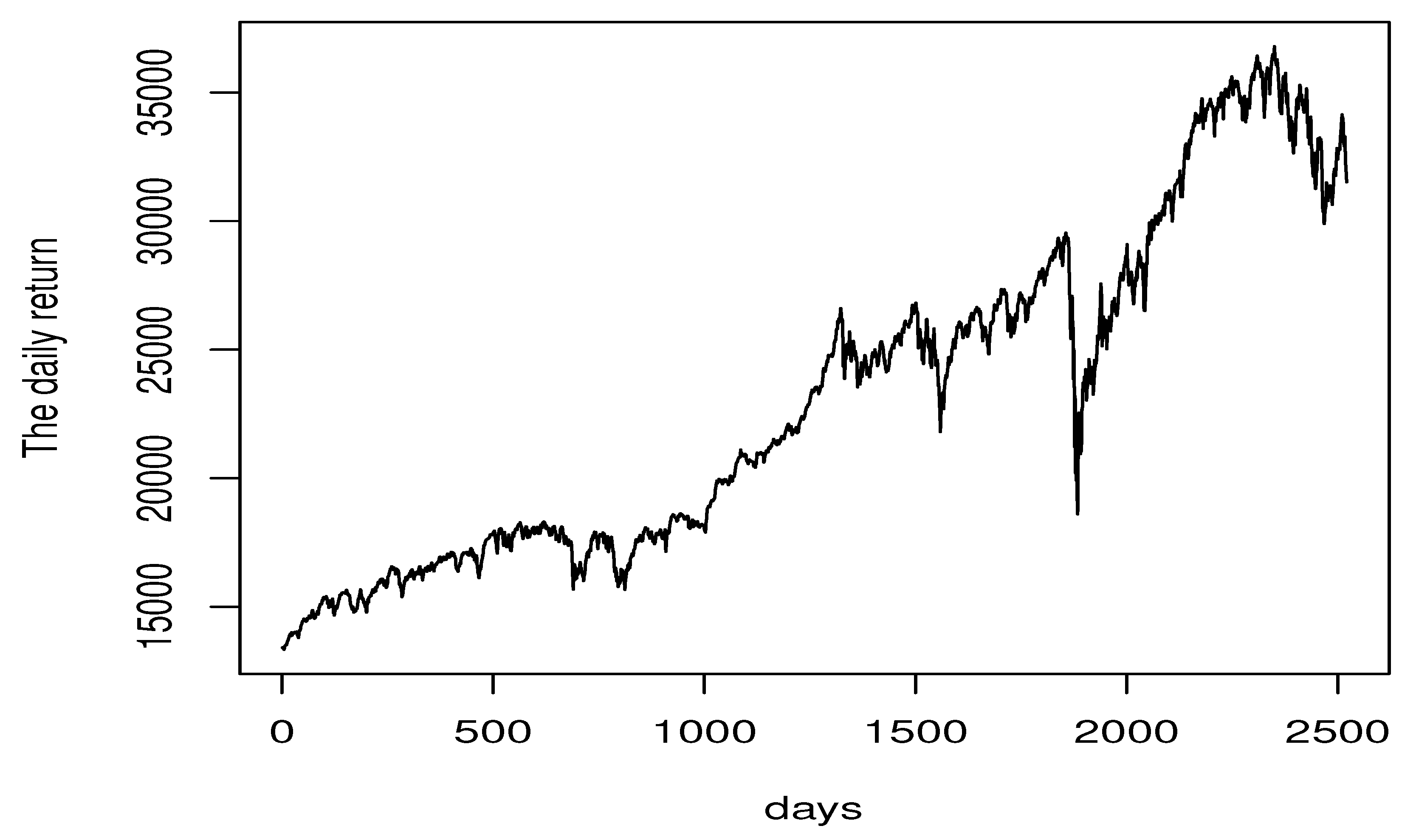
This comparison study is carried out by employing an experiment over real financial data. More precisely, we consider the log daily return of the Dow Jones Industrial stock index between 1 January 2013 to 31 August 2022. Specifically, we proceed with the process Z ( t ) = 100 log r ( t ) r ( t 1 ) . The data of this real example can be accessed through the website https://fred.stlouisfed.org/series/DJIA (accessed on 14 September 2022). After prior analysis, we observe that the considered financial data exhibit the fundamental features of financial time series data, such as skewness, excess kurtosis, and high volatility. In Figure 2, we plot the initial data without transformation.
It is well known the continuous time process is the principal source of functional statistics. We can easily construct the functional variable by cutting the trajectory of this process over small intervals. We employ this idea and take the functional regressor X ( · ) equal to the values of Z (over one month) and its associated real interest variable Y is equal to Z (at the last day of the month).
Now, we compute the efficiency of the recursive estimator by computing the percentage of the violation cases corresponding to the situation when the process z ( t ) exceeds the estimator. Let us clarify that the computation ability of the estimator is also affected by the choice of the distance d. However, the metric choice depends on the regularity and on the smoothness of the regressor curves. Therefore, in this heteroscedastic, when the regressor curves are discontinuous, the PCA metric is more adequate than the functional spline metric. This is our principal motivation to compute our estimator using this metric. Finally, we note that we used the quadratic kernel on ( 0 , 1 ) , and therefore we have split the data into 70 % of observations in the learning sample and 30 % of observations. We plot the true values of the process at the testing observation versus its estimated values using the three selector procedures (see Figure 3).
It is clear that the choice of the smoothing parameters ( h i ) i has a great impact on the performance of the estimator E ^ p ( x ) . This statement is confirmed by the high variability of the percentage of the violation cases with respect to the selection method. In particular, selector 1 gives 4.3% of violation cases while percentages equal to 2.5% and 3.8% are obtained by selector 2 and selector 3, respectively. Among the three selector algorithms, it appears that the procedure of selector 2 is more preferred than the other algorithm. Finally, we can say that the recursive estimator is very easy to implant in practice, and its efficiency, without surprise, is strongly affected by the determination of the smoothing parameter h i .

6. Conclusions

We consider, in this work, functional ergodic time series and construct a recursive estimator for the conditional expectile. The asymptotic property of the established estimator is proved using standard conditions covering the principal structures of this work, such as the functional ergodicity assumption, the recursivity, and the nonparametric aspect of the model. The applicability of this estimator and its feasibility are evaluated using artificial and real data. This computational part emphasizes the importance of this estimator in practice as a fast estimator allowing the update of the results for each new piece of information. Such a feature is the principal gain of the recursive property of our estimator. In addition to these results, we have particularized our study to some special cases. Thus, we can say that the generality of our approach is also an essential feature of the proposed estimator. In addition, the present contribution also opens some interesting paths for the future. For example, it will be interesting to construct the asymptotic normality of our proposed recursive estimator to extend the obtained result to incomplete data, including missing, censored, or truncated data. Another possible future track is treating more complicated dependence structures such as the ergodic spatial dependence or the quasi-association functional random fields.

Author Contributions

The authors contributed approximatily equally to this work. Formal analysis, F.A.; Validation, Z.C.E. and Z.K.; Writing—review & editing, I.M.A., A.L. and M.R. All authors have read and agreed to the published version of the manuscript.

Funding

This research project was funded by the Deanship of Scientific Research, Princess Nourah bint Abdulrahman University, through the Program of Research Project Funding after Publication, grant No. (43-PRFA-P-25).

Institutional Review Board Statement

Not applicable.

Informed Consent Statement

Not applicable.

Data Availability Statement

The data used in this study are available through the link https://fred.stlouisfed.org/series/DJIA (accessed on 14 September 2022).

Acknowledgments

The authors thank and extend their appreciation to the Deanship of Scientific Research, Princess Nourah bint Abdulrahman University for funding this work.

Conflicts of Interest

The authors declare no conflict of interest.

Appendix A

Proof of Lemma 1.
 
The compactness of [ E p ( x ) δ , E p ( x ) + δ ] permits to have [ E p ( x ) δ , E p ( x ) + δ ] j = 1 d n y j n , y j + n with n = n 1 / 2 and d n = O n 1 / 2 . Let
G n = y j n , y j + n , 1 j d n .
The monotony of G ^ N ( l , · ; x ) and G ¯ N ( l , · ; x ) gives, for all 1 j d n ,
G ^ N ( l , ( y j n ) ; x ) sup y ( y j n , y j + n ) G ^ N ( l , ( y j n ) ; x ) G ^ N ( l , ( y j n ) ; x )
and
G ¯ N ( l , ( y j n ) ; x ) sup y ( y j n , y j + n ) G ¯ N ( l , ( y j n ) ; x ) G ¯ N ( l , ( y j n ) ; x ) .
Using (A2) and by the same arguments as in Lemma 3, we deduce that, for y 1 , y 2 [ E p ( x ) δ , E p ( x ) + δ ] ,
G ¯ N ( l , ( y j n ) ; x ) G ¯ N ( l , ( y j n ) ; x ) C | y 1 y 2 | 1 i = 1 n ϕ x 1 l ( h i ) i = 1 n C i ϕ x 1 l ( h i ) ,
and hence,
sup y [ E p ( x ) δ , E p ( x ) + δ ] G ^ N ( l , ( y j n ) ; x ) G ¯ N ( l , ( y j n ) ; x )
max 1 j d n max z { y j n , y j + n } G ^ N ( l , z ; x ) G ¯ N ( l , z ; x ) + 2 C n almost   completely .
Observe that, under (A4)
n = o log n n ϕ x ( h n ) .
Therefore, to finalize this lemma proof, it is be sufficient to show that
max 1 j d n max z { y j n , y j + n } G ^ N ( l , z ; x ) G ¯ N ( l , z ; x ) = O a.co. log n n ϕ x ( h n ) .
To accomplish that, it is sufficient to consider the fact that
I P max z G n G ^ N ( l , z ; x ) G ¯ N ( l , z ; x ) > ε z G n I P G ^ N ( l , z ; x ) G ¯ N ( l , z ; x ) > ε .
Because Y does not have to be bounded, a truncation procedure is used by introducing the function:
G ^ N ( l , z ; x ) = 1 i = 1 n ϕ x 1 l ( h i ) i = 1 n 1 ϕ x l ( h i ) K i ( x ) Y i
G ¯ N ( l , z ; x ) = 1 i = 1 n ϕ x 1 l ( h i ) i = 1 n 1 ϕ x l ( h i ) I E K i ( x ) Y i | G i 1 ,
where
Y i = Y i 1 I { | Y | < γ n } ,
with γ n = n a / q . Hence, the following three results accomplish the above claimed result:
d n max z G n G ¯ N ( l , z ; x ) G ¯ N ( l , z ; x ) = O a.co. log n n ϕ x ( h n ) ,
d n max z G n G ^ N ( l , z ; x ) G ^ N ( l , z ; x ) = O a.co. log n n ϕ x ( h n )
and
d n max z G n G ^ N ( l , z ; x ) ( x , z ) G ¯ N ( l , z ; x ) = O a.co. log n n ϕ x ( h n ) .
Let us consider the statement (A1). We have, for all z G n ,
G ¯ N ( l , z ; x ) G ¯ N ( l , z ; x ) C 1 i = 1 n ϕ x 1 l ( h i )
i = 1 n 1 ϕ x l ( h i ) I E Y i 1 I { | Y i | γ n } K ( h i 1 d ( x , X i ) ) | G i 1 .
Apply Hölder inequality, for α = p 2 with β such that
1 α + 1 β = 1 .
Use (A1) and (A5) to show that, for all  z G n ,
I E Y i 1 I { | Y i | γ n } K ( h i 1 d ( x , X i ) ) | G i 1 I E 1 / α Y i α 1 I { | Y i | γ n } | G i 1 I E 1 / β K i β ( x ) | G i 1 γ n 1 I E 1 / α Y i 2 α | G i 1 I E 1 / β K i β ( x ) | G i 1 γ n 1 I E 1 / α Y p | G i 1 I E 1 / β K i β ( x ) | G i 1 C γ n 1 ϕ i 1 / β ( x , h i ) C i γ n 1 ϕ x 1 / β ( h i ) .
Hence, we obtain under (A4)
d n max z G n G ¯ N ( l , z ; x ) G ¯ N ( l , z ; x ) C n 1 / 2 a / q ϕ x ( 1 β ) / β ( h n ) .
Using the fact that a > p / 2 , we obtain the statement (A1). Next, Markov’s inequality is used to prove (A2), that, z G n , ϵ > 0 ,
I P G ^ N ( l , z ; x ) G ^ N ( l , z ; x ) > ϵ i = 1 n I P | Y i | > n a / q n I P | Y i | > n a / q n 1 a I E Y p .
Because of (A4) and the fact that a > 3 , we have
d n max z G n I P G ^ N ( l , z ; x ) ( x , z ) G ¯ N ( l , z ; x ) > ϵ 0 log n n ϕ x ( h n ) n 3 / 2 a < C n 1 ν for ν > 0 .
We now prove (A3). To this end, we define, for all z G n ,
Now, for any z G n set
Λ i ( l , z ; x ) = 1 ϕ x l ( h i ) K i ( x ) Y i I E K i ( x ) Y i | G i 1 .
The rest of the proof is based on the same exponential inequality used in previous Lemma 1. As
| Λ i ( l , z ; x ) | C γ n ϕ x l ( h n )
So all it remains to evaluate asymptotically the conditional variance of Λ i ( l , z ; x ) .
I E K i Y i 2 | G i 1 = I E I E | K i | 2 | Y i | 2 | X | G i 1 = I E I E | Y i | 2 | X K i 2 | G i 1 = C I E K i 2 | G i 1 ,
By using the assumptions (H2), (H3) we obtain
I E K i Y i 2 | G i 1 C ϕ i ( x , h i ) C i ϕ x ( h i ) .
We therefore obtain, under (A4) that
i = 1 n I E Λ i 2 ( l , z ; x ) = O ϕ x 1 2 l ( h n ) .
Hence, use the martingale-difference inequality of (see Laib and Louani [8], p. 365) to fulfill this proof. Therefore, we obtain, for all η > 0 and for all z G n ,
I P G ^ N ( l , z ; x ) G ¯ N ( l , z ; x ) > η log n n ϕ x ( h n )
I P i = 1 n Λ i ( l , z ; x ) > η i = 1 n ϕ x 1 l ( h i ) log n n ϕ x ( h n )
2 exp 1 2 η 2 i = 1 n ϕ x 1 l ( h i ) 2 log n n ϕ x ( h n ) C i = 1 n ϕ x 1 2 l ( h i ) + γ n i = 1 n ϕ x 1 l ( h i ) ϕ x l ( h n ) log n n ϕ x ( h n ) .
2 exp C 2 η 2 n ϕ x 1 l ( h n ) 2 log n n ϕ x ( h n ) C n ϕ x 1 2 l ( h n ) + γ n n ϕ x 1 l ( h n ) ϕ x l ( h n ) log n n ϕ x ( h n ) .
2 exp C 2 η 2 n ϕ x 1 l ( h n ) 2 log n n 2 ϕ x 2 2 l ( h n ) C + γ n ϕ x l ( h n ) ϕ x l ( h n ) log n n ϕ x ( h n ) .
2 exp C 2 η 2 log n C + γ n ϕ x l ( h n ) ϕ x l ( h n ) log n n ϕ x ( h n ) .
Then, as d n C n 1 , we have
z G n I P G ^ N ( l , z ; x ) G ¯ N ( l , z ; x ) > η log n n ϕ x ( h n ) 2 d n max z G n I P G ^ N ( l , z ; x ) G ¯ N ( l , z ; x ) > η log n n ϕ x ( h n ) C n C η 2 + 1 / 2 .
Thus, a suitable choice of η leads to the proof of the first statement of this lemma. The second one is obtained by a similar way. □
Proof of Lemma 2.
 
Using the same ideas of Ferraty et al. (2007) to prove, under (H1) (iii) and (H3), there exists C t , x > C > 0 such that
sup t [ E p ( x ) δ , E p ( x ) + δ ] G ¯ D ( l , t ; x ) C t , x = o a.co. ( 1 ) .
It is easy to see that,
inf t [ E p ( x ) δ , E p ( x ) + δ ] G ¯ D ( l , t ; x ) C t , x 2
t 0 [ E p ( x ) δ , E p ( x ) + δ ] , such   that C t 0 , x G ¯ D ( l , t 0 ; x ) > C t 0 , x 2
sup t [ E p ( x ) δ , E p ( x ) + δ ] | C t , x G ¯ D ( l , t ; x ) | > C t , x 2 .
We deduce from Equation (A5) that
P inf t [ E p ( x ) δ , E p ( x ) + δ ] G ¯ D ( l , t ; x ) C t , x 2 P sup t [ E p ( x ) δ , E p ( x ) + δ ] | C t , x G ¯ D ( l , t ; x ) | > C t , x 2 .
Consequently,
i = 1 inf t [ E p ( x ) δ , E p ( x ) + δ ] G ¯ D ( l , t ; x ) C t , x 2 < .
Proof of Lemma 3.
Clearly
B ^ n ( t ; x ) 1 G ¯ D ( l , t ; x ) i = 1 n ϕ x 1 l ( h i ) i = 1 n ϕ x l ( h i ) I E K i ( x ) | G 1 ( t ; X i ) G 2 ( t ; X i ) G ( t ; x ) | | G i 1 .
It is clear that
| G 1 ( t ; X i ) G 2 ( t ; X i ) G ( t ; x ) | | G 1 ( t ; X i ) G 1 ( t ; x ) | + | G ( t ; x ) | | G 2 ( t ; X i ) G 2 ( t ; x ) |
using (H2), we obtain, for all t [ E p ( x ) δ , E p ( x ) + δ ]
1 I B ( x , h i ) ( X i ) | G 1 ( t ; X i ) G 1 ( t ; x ) | C h i β 1 .
and
1 I B ( x , h i ) ( X i ) | G 2 ( t ; X i ) G 2 ( t ; x ) | C h i β 2 .
Combining these approximations with the statement with the Lemma 2 to write that
sup t [ E p ( x ) δ , E p ( x ) + δ ] | B ^ n ( t ; x ) | C 1 i = 1 n ϕ x 1 l ( h i ) i = 1 n C i ( h i β 1 + h i β 2 ) ϕ x 1 l ( h i )
Hence, we conclude that
sup t [ E p ( x ) δ , E p ( x ) + δ ] | B ^ n ( t ; x ) | = O a.co. h n min ( β 1 , β 2 )

References

  1. Amiri, A.; Crambes, C.; Thiam, B. Recursive estimation of nonparametric regression with functional covariate. Comput. Stat. Data Anal. 2014, 69, 154–172. [Google Scholar] [CrossRef] [Green Version]
  2. Ardjoun, F.; Ait Hennani, L.; Laksaci, A. A recursive kernel estimate of the functional modal regression under ergodic dependence condition. J. Stat. Theory Pract. 2016, 10, 475–496. [Google Scholar] [CrossRef]
  3. Benziadi, F.; Laksaci, A.; Tebboune, F. Recursive kernel estimate of the conditional quantile for functional ergodic data. Commun. Stat. Theory Methods 2016, 45, 3097–3113. [Google Scholar] [CrossRef]
  4. Slaoui, Y. Recursive nonparametric regression estimation for independent functional data. Stat. Sin. 2020, 30, 417–437. [Google Scholar] [CrossRef]
  5. Slaoui, Y. Recursive nonparametric regression estimation for dependent strong mixing functional data. Stat. Inference Stoch. Process. 2020, 23, 665–697. [Google Scholar] [CrossRef]
  6. Laksaci, A.; Khardani, S.; Semmar, S. Semi-recursive kernel conditional density estimators under random censorship and dependent data. Commun. Stat. Theory Methods 2022, 51, 2116–2138. [Google Scholar] [CrossRef]
  7. Laïb, N.; Louani, D. Nonparametric kernel regression estimate for functional stationary ergodic data: Asymptotic properties. J. Multivariate Anal. 2010, 101, 2266–2281. [Google Scholar] [CrossRef] [Green Version]
  8. Laïb, N.; Louani, D. Rates of strong consistencies of the regression function estimator for functional stationary ergodic data. J. Stat. Plan. Inference 2011, 141, 359–372. [Google Scholar] [CrossRef]
  9. Gheriballah, A.; Laksaci, A.; Sekkal, S. Nonparametric M-regression for functional ergodic data. Stat. Probab. Lett. 2013, 83, 902–908. [Google Scholar] [CrossRef]
  10. Pratesi, M.; Ranalli, M.G.; Salvati, N. Nonparametric M-quantile regression using penalised splines. J. Nonparametr. Stat. 2009, 21, 287–304. [Google Scholar] [CrossRef]
  11. Waltrup, L.S.; Sobotka, F.; Kneib, T.; Kauermann, G. Expectile and quantile regression—David and goliath? Stat. Model. 2015, 15, 433–456. [Google Scholar] [CrossRef] [Green Version]
  12. Farooq, M.; Steinwart, I. Learning rates for kernel-based expectile regression. Mach. Learn. 2019, 108, 203–227. [Google Scholar] [CrossRef] [Green Version]
  13. Daouia, A.; Paindaveine, D. From halfspace m-depth to multiple-output expectile regression. arXiv 2019, arXiv:1905.12718. [Google Scholar]
  14. Mohammedi, M.; Bouzebda, S.; Laksaci, A. The consistency and asymptotic normality of the kernel type expectile regression estimator for functional data. J. Multivariate Anal. 2021, 181, 104673. [Google Scholar] [CrossRef]
  15. Almanjahie, I.; Bouzebda, S.; Chikr Elmezouar, Z.; Laksaci, A. The functional kNN estimator of the conditional expectile: Uniform consistency in number of neighbors. Stat. Risk Model. 2022, 38, 47–63. [Google Scholar] [CrossRef]
  16. Roussas, G.; Tran, L.T. Asymptotic normality of the recursive kernel regression estimate under dependence conditions. Ann. Stat. 1992, 20, 98–120. [Google Scholar] [CrossRef]
  17. Almanjahie, I.; Bouzebda, S.; Kaid, Z.; Laksaci, A. Nonparametric estimation of expectile regression in functional dependent data. J. Nonparametr. Stat. 2022, 34, 250–281. [Google Scholar] [CrossRef]
  18. Wolverton, C.T.; Wagner, T.J. Asymptotically optimal discriminant functions for a pattern classification. IEEE Trans. Inf. Theory 1969, 15, 258–265. [Google Scholar] [CrossRef]
  19. Yamato, H. Sequential estimation of a continous probability density funciton and mode. Bull. Math. Stat. 1971, 14, 1–12. [Google Scholar] [CrossRef]
  20. Bouzebda, S.; Slaoui, Y. Nonparametric recursive method for moment generating function kernel-type estimators. Stat. Probab. Lett. 2022, 184, 109422. [Google Scholar] [CrossRef]
  21. Slaoui, Y. Moderate deviation principles for nonparametric recursive distribution estimators using Bernstein polynomials. Rev. Mat. Complut. 2022, 35, 147–158. [Google Scholar] [CrossRef]
  22. Jones, M.C. Expectiles and M-quantiles are quantiles. Stat. Probab. Lett. 1994, 20, 149–153. [Google Scholar] [CrossRef]
  23. Abdous, B.; Rémillard, B. Relating quantiles and expectiles under weighted-symmetry. Ann. Inst. Stat. Math. 1995, 47, 371–384. [Google Scholar] [CrossRef]
  24. Bellini, F.; Bignozzi, V.; Puccetti, G. Conditional expectiles, time consistency and mixture convexity properties. Insurance Math. Econom. 2018, 82, 117–123. [Google Scholar] [CrossRef]
  25. Girard, S.; Stupfler, G.; Usseglio-Carleve, A. Extreme conditional expectile estimation in heavy-tailed heteroscedastic regression models. Ann. Stat. 2021, 49, 3358–3382. [Google Scholar] [CrossRef]
  26. So, M.K.P.; Chu, A.M.Y.; Lo, C.C.Y.; Ip, C.Y. Volatility and dynamic dependence modeling: Review, applications, and financial risk management. Wiley Interdiscip. Rev. Comput. Stat. 2022, 14, e1567. [Google Scholar] [CrossRef]
  27. Feng, Y.; Beran, J.; Yu, K. Modelling financial time series with SEMIFAR-GARCH model. IMA J. Manag. Math. 2007, 18, 395–412. [Google Scholar] [CrossRef]
  28. Bogachev, V.I. Gaussian Measures: Mathematical Surveys and Monographs; American Mathematical Society: Providence, RI, USA, 1999; Volume 62. [Google Scholar]
  29. Ferraty, F.; Vieu, P. Nonparametric Functional Data Analysis; Springer Series in Statistics. Theory and Practice; Springer: New York, NY, USA, 2006. [Google Scholar]
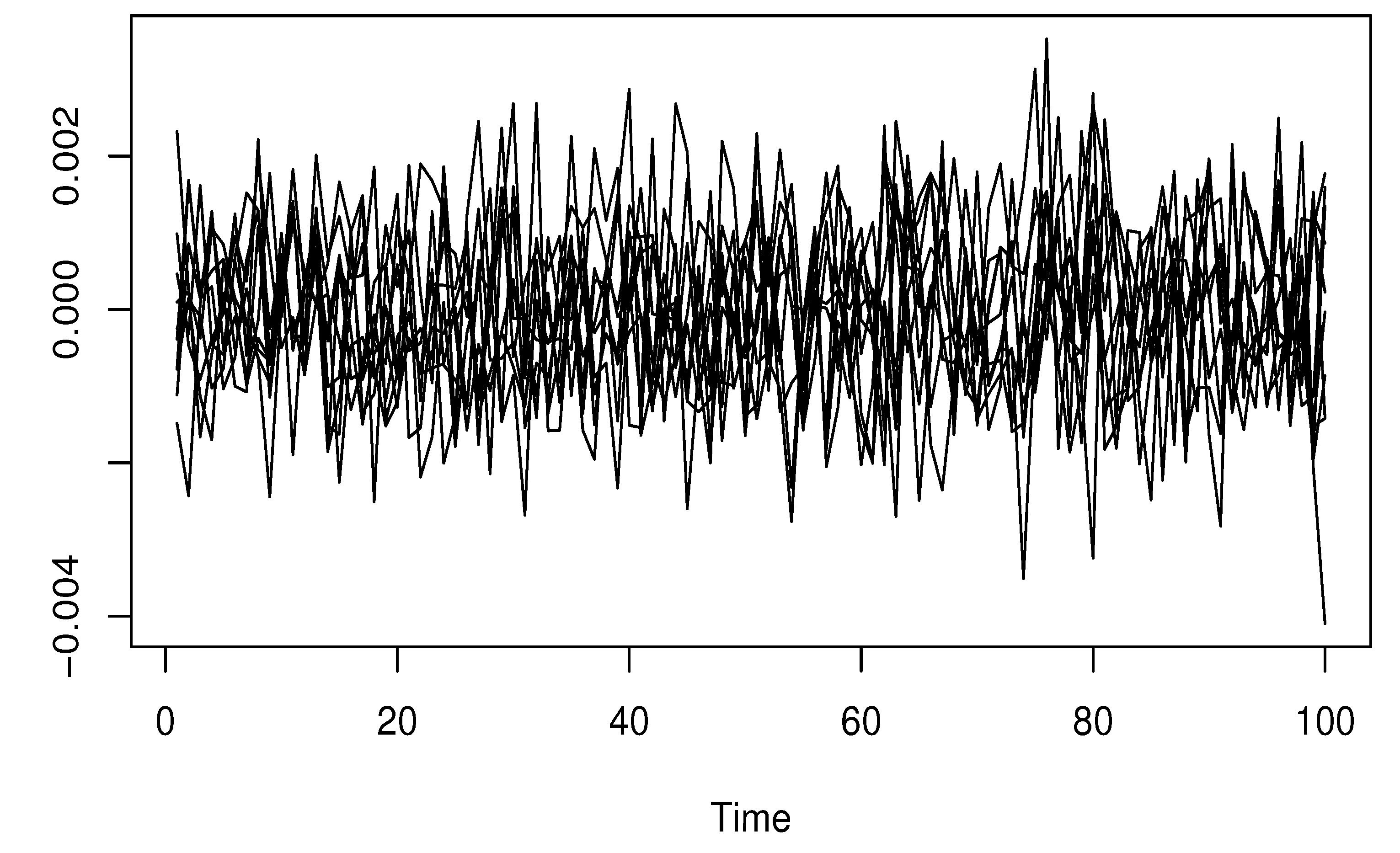
Figure 1. The functional regressors.
Mathematics 10 03919 g001
Figure 2. The Log daily return of the Dow Jones Industrial stock index.
Mathematics 10 03919 g002
Figure 3. Comparison between the three selectors of the recursive estimator of the conditional expectile for order p = 0.01 .
Mathematics 10 03919 g003
Table 1. A S E results.
DistributionpNE (l = 0)NE (l = 0.5)NE (l = 1)CKE
Log-normal distribution0.10.140.120.180.69
0.10.140.120.180.69
0.50.090.050.080.23
0.90.170.150.160.57
Normal distribution0.10.190.220.240.87
0.50.040.10.080.75
0.90.230.280.210.96
Exponential distribution0.10.120.170.130.45
0.50.020.090.060.39
0.90.170.250.240.77
Publisher’s Note: MDPI stays neutral with regard to jurisdictional claims in published maps and institutional affiliations.