
Fault-Tolerant Control for Quadrotor Based on Fixed-Time ESO
by
 ,
,
Lei Liu
1,†,
Junjie Liu
1,†,
Junfang Li
1,*,
Yuehui Ji
1,
Yu Song
1,
Liang Xu
1 and
Wenxing Niu
2 1
Tianjin Key Laboratory for Control Theory and Applications in Complicated Industry Systems, School of Electrical Engineering and Automation, Tianjin University of Technology, Tianjin 300384, China
2
Tianjin Enpromi Environmental Protection Technology Co., Ltd., Tianjin 300462, China
*
Author to whom correspondence should be addressed.
†
These authors contributed equally to this work.
Mathematics 2022, 10(22), 4386; https://doi.org/10.3390/math10224386
Submission received: 9 October 2022
/
Revised: 9 November 2022
/
Accepted: 15 November 2022
/
Published: 21 November 2022
Abstract
:Focusing on the actuator fault of the quadrotor unmanned aerial vehicle (QUAV), an active fault-tolerant control scheme based on fixed-time linear active disturbance rejection control is proposed. Firstly, in order to simplify the complex dynamic model, the virtual control quantity is introduced to decouple the flight control system of the QUAV. Secondly, the fixed-time extended state observer (ESO) is utilized to estimate and compensate the internal uncertainty, external disturbance and actuator fault of the QUAV in fixed time. Thirdly, a continuous output feedback controller based on fixed-time ESO is designed to keep the stability of the flight control system with actuator fault and external disturbance. Finally, the closed-loop stability of the flight control system is demonstrated by Lyapunov function. The numerical simulation is carried and the results also verify the effectiveness of the proposed control scheme.
Keywords:
actuator fault; external disturbance; fault-tolerant control; fixed-time ESO; quadrotor; UAVMSC:
68M15; 68T40; 70E60; 70Q05; 93-XX; 93-10; 93B52; 93B53; 93C10; 93C40; 93DXX; 94C121. Introduction
Quadrotor unmanned aerial vehicle (QUAV) is a multi-rotor remote control autonomous flight vehicle, which can achieve vertical take-off and landing [1], and quickly change flight attitude in narrow space [2]. Therefore, QUAV has a wide application prospect in agricultural production [3], atmospheric monitoring [4], forest fire prevention [5], electric power inspection [6] and so on.
In order to realize the autonomous flight and high reliability mission requirements of QUAV, attitude and path tracking control is the most important technology. However, the QUAV flight control system has the characteristics of nonlinearity, under-actuation, strong coupling [7] and mathematical model uncertainty [8]. In addition, the QUAV will still have some unexpected faults in actual flight process [9]. From the view of fault location, the fault can be divided into sensor fault, actuator fault and structural fault. Among them, sensor fault and structural fault are mainly related to internal components. With the improvement of microelectronics technology and the existence of redundant configuration in QUAV, the probability of these two types of faults is relatively low, while the frequency of actuator fault is higher [10], which is 44% [11]. The actuator is a structure that converts the signal generated by the system controller into an electrical signal to change the position and attitude. Therefore, whether the actuator is perfect and effective has a great impact on the stability of the whole system.
The idea of fault-tolerant control can be traced back to 1971 and developed from [12] integrity control proposed by Professor Niederlinski. Since then, the system fault-tolerant control technology has attracted the attention of scholars and experts [13,14]. According to the method of system implementation, fault-tolerant control can be divided into two types: the hardware redundancy method and analytical redundancy method. However, the method of hardware redundancy increases the complexity of QUAV control and structure to a great extent. With the development of fault-tolerant control technology and the progress of aviation technology, analytical redundancy has gradually developed [15]. Analytical redundancy can be subdivided into passive fault-tolerant control and active fault-tolerant control [16]. For the passive fault-tolerant control system, the fault information is taken into account as a priori knowledge before the design of the control law, so it does not include the fault diagnosis and isolation module. The system has faster response speed and good robustness. The traditional methods include quantitative feedback theory [17], H∞ algorithm [18,19] and backstepping control algorithm [20]. However, it is difficult to get a good control effect for unknown faults. While the active fault-tolerant control method does not need to know the fault information in advance, especially for unknown system faults, the control effect is better and has a wider range of application.
At present, there are many research results on active fault-tolerant control of aircraft flight control systems. The commonly utilized control methods include feedback linearization [21], backstepping [22], PID control [23], nonlinear adaptive fault-tolerant control technology [24], fault-tolerant control based on fault diagnosis observer [25] and predictive fault-tolerant control [26]. Considering the fault-tolerant control in the case of actuator fault in the aircraft, Xiao [27] and Zhang [28] constructed the attitude and speed control law through the sliding mode observer to realize the stability of the attitude control subsystem, but did not consider the tracking control of the position trajectory subsystem. Zhao [29] designed an adaptive unknown input observer to estimate the uncertain parameters of actuator fault and realized the stability of the attitude subsystem, but did not analyze the actuator fault model. When the external disturbance occurs, this method will not be applicable. Aiming at the tracking control problem of aircraft in the presence of external disturbance from air resistance, Li [30] designed a sliding mode fault-tolerant controller to deal with two kinds of problems: propeller damage and actuator fault in quadrotor QUAV, but it cannot analyze the sudden disturbance from the wireless communication of the system. Wang [31] designed a control strategy based on adaptive and sliding mode control to realize the attitude tracking control of QUAV, but the position trajectory tracking control was not considered. Razmi [32] realized the stability control of quadrotor UAV by the combination of neural network and adaptive sliding mode control. However, the complexity of neural network parameter solution limited the application in practical engineering. Zeghlache [33] proposed an algorithm by combining the backstepping control and the fuzzy sliding mode control to realize the attitude control of the quadrotor helicopter. When the fault or external disturbance occurred in the system, the control performance of this method would be obviously insufficient. In addition, Gong [34] designed an adaptive sliding mode control method to compensate the faults and uncertainties, but only studied the attitude control subsystem and the analysis was not comprehensive. Nekoukar [35] proposed a controller design scheme combining proportional differential control and terminal sliding mode control algorithm, but did not consider the position tracking control. Yang [36] applied the nonsingular terminal sliding mode control algorithm to the attitude fault-tolerant control, but the influence of disturbance on the aircraft was not considered. A hybrid fault detection and isolation scheme was designed in [37] to deal with large environmental disturbances and actuator faults while this solution relied on the precise mathematical model.
It can be seen from the above research results that the research on fault-tolerant control of aircraft has become a hot topic. However, due to the complexity constraints of the QUAV system model, most of the research results remain in the stability analysis of the attitude controller. Moreover, many research results are realized in the ideal environment, and the influence of external disturbance is ignored. Therefore, the designed fault-tolerant controller should not only effectively ensure the stability of the system in the case of system fault, but also be effective in the case of external disturbance.
In addition, in many applications, understanding the current state of the dynamic system is essential for constructing the controller or attaining the real time information about the system for monitoring or decision-making. Furthermore, since this research, many disturbance observers have been studied, such as the typical asymptotic disturbance observer [38], the exponential observer [38], the typical finite-time disturbance observer [38], robust observer [38], Kalman or Kalman-like observers [38], high-gain observers [38], adaptive observers [38], first-order and high-order sliding-mode observers [39] and classic ESO [40]. The function of the observer is to estimate the state of the equipment in real time based on the information of its output. This means that the signal contains enough information in some way to uniquely determine the overall state of the system.
Additionally, due to the complex structure of the QUAV, it is difficult to establish the precise dynamics model. However, active disturbance rejection control (ADRC) is a hot control algorithm. Professor Han first proposed the ADRC, which is not highly dependent on the model. Before long, Professor Gao proposed the linear ADRC to solve the problem of too many parameters in ADRC. Also, to deal with some difficult control problems in the QUAV system, such as nonlinearity, strong coupling and sensitive to disturbance, Yong Zhang proposed a kind of double closed-loop ADRX scheme.
Then, in order to make up for the deficiencies of above methods and improve the fault-tolerant control performance of QUAV, on the basis of the ADRC, the fault-tolerant controller based on fixed-time extended state observer (ESO) is designed for the dynamic system of the QUAV, including actuator fault and disturbance.
Compared with other control methods, the fixed-time control method has many advantages and has attracted more and more attention. Compared with the finite-time observer mentioned above, the fixed-time ESO can estimate the state of the flight control system in real time and compensate the effects of disturbances, model uncertainties and faults in fixed time. It can be said that the fixed-time ESO is equivalent to the fast subsystem, which not only ensures the fast convergence of the observer, but also ensures sufficiently high estimation accuracy and provides a valuable and available speed signal for the system. It has strong robustness to the parametric uncertainties, and the convergence time of the fixed-time ESO has an upper bound. It is not influenced by the initial estimation error and external disturbances of dynamic systems and does not rely on the precise mathematical model. In addition, it is insensitive to system state changes and has been widely used in automated systems. The observation and disturbance rejection capability are greatly improved.
Here, this paper focuses on the active fault-tolerant control of QUAV with partial actuator fault and designs the corresponding fixed-time observer and controller. The main work of this paper is as follows:
- A fixed-time ESO is proposed to estimate and compensate the internal uncertainty, external disturbance and actuator fault of QUAV in fixed time. In contrast with other finite-time convergence ESO, the convergence time of fixed-time ESO has an upper bound and it is not influenced by the initial estimation error. The observation and disturbance rejection capability are greatly improved.
- A fixed-time continuous output feedback controller is proposed to keep the system stable quickly in fixed time and the convergence time is independent of initial conditions. Different from other multi-variable decoupling control methods, the controllers are devised independently in each channel and the strong couplings among different channels are basically eliminated. With the well previously designed fixed-time ESO, the actuator fault, external disturbance, internal uncertainty and the unmodeled dynamics are extended into a new state, which is considered as the overall disturbance and can be estimated and compensates in fixed time.
- Multiple actuator partial loss-of-effectiveness faults and external disturbance are both considered in the model of QUAV. Besides, based on fixed-time ESO, the initial system dynamic can be simplified to an integrator system.
2. System Dynamics Model
QUAV is a kind of 6 degrees of freedom and under actuated rotary aircraft. The flight attitude and position are changed by adjusting the rotor speed. The center of gravity of the QUAV is at its geometric center. The four rotors of the QUAV generate the power, which is directly proportional to the square of the angular velocity of rotor rotation. The continuous high-speed rotation of the motor and propeller will greatly improve the probability of fault.
2.1. Fault-Free Model
The force analysis diagram is shown in Figure 1.
According to the flight principle of QUAV and the coordinate system conversion relationship, the flight dynamics model of QUAV is constructed as follows [41].
where , and are the position variables of the QUAV. , and are the pitch angle, roll angle and yaw angle, respectively. is the mass of the QUAV. is the gravitational acceleration. is the air resistance coefficient. is the rotational inertia of the axis. is the rotational inertia of the axis. is the rotational inertia of the axis. Four virtual control variables of the whole system are introduced. Also, in the position loop, are the virtual control inputs.
The actual control input of altitude Z channel in the position loop can be calculated as below:
In the same way, the expected intermediate values of the pitch angle and roll angle are calculated by the inverse solution below:
Then, the typical fault-free dynamic model of QUAV is established well.
2.2. Fault Model
With the use of mechanical equipment, the performance will deteriorate, and the actual force and torque will decrease. According to the degree of fault occurrence, the actuator fault can be divided into partial fault and complete fault. Partial fault belongs to the type of multiplicative fault that the actuator output defects but not completely loses of function. Complete fault means the actuator loses the effectiveness completely. No matter what input, the actuator will not operate.
The partial fault of actuator in QUAV flight control system is mainly studied in this article. Because of the high frequency of such fault, is not easy to be found. To some extent, it has a great impact on the flight control system.
Therefore, partial actuator fault can be described as the change of control input to facilitate the unified description and the establishment of fault model. Then the influence of partial actuator fault on control input synthesis can be expressed by introducing unknown effectiveness factor. is introduced as the unknown effectiveness factor of actuators, which satisfy .
In addition, the unknown disturbances from the external environment are added to the system. Then, the fault model of QUAV can be rewritten as follows:
where the initial values of the external disturbances are set as follows:
and
Then, the fault dynamic model of QUAV is established well.
3. Control Scheme
In order to realize the better path tracking performance of the QUAV, the flight control system is divided into four separate channels: the yaw angle channel, the altitude channel, the cascade channel and the cascade channel. The design of cascade controller is introduced in detail in the later section. The position is considered as the control input in the pitch angle channel, while the position is considered as the control input in the roll angle channel. The design scheme of QUAV is shown in the Figure 2 below.
Using the above model, the fixed-time ESO is designed. Then, the internal uncertainty, external disturbance and unknown fault disturbance of the system are estimated and compensated in fixed time. In addition, the fixed-time continuous output feedback controller is design based on linear active disturbance rejection control. The expected values of pitch angle and roll angle can be obtained by the inverse solution calculation of control quantity to improve the control precision and meet the performance needs under the normal and fault conditions.
According to Equation (5), define
3.1. Position Control by Composite Controller
Before the beginning of this section, a notation is given as below.
Notation 1.
In this article, define, here is the symbolic function and .
3.1.1. Controller Design for Yaw Angle Channel
In this separate channel, the reference input is the desired value . Then, the virtual control variable can be attained. By combining Equation (8), the expression of yaw angle in Equation (5) can be rewritten as follows in Equation (9):
where is the derivative of the total disturbance in the yaw angle channel. Then the original dynamics can be approximated as a second-order integrator system with a total disturbance. The total disturbance makes the system stay away from the expected second-order integrator. Estimating and eliminating the total disturbance is the solution.
The ESO and the controller designed in [40] are as follows:
A more specific design process is described in reference [40].
However, in this article, by applying the high-order sliding mode technology, the fixed-time ESO for the yaw angle channel is designed as follows in Equation (11):
where are the observed values of , the differential signal of and the total disturbance of the yaw angle channel, respectively. The output of the yaw angle channel is are the observer gains. and meet and are the adjustable observer parameters related to the system. In simulations, a continuous hyperbolic tangent function will substitute for to avoid chattering. are the estimation errors of the fixed-time ESO, the differential of which can be expressed as below:
Lemma 1.
For the yaw angle in dynamic system, if the fixed-time ESO is designed as shown in Equation (11), then there exists a constant numberand proper parameters, which means the state variablescan be estimated bywithin the fixed time. Furthermore, the estimation error of total disturbancecan also converge to a neighborhood of the origin within the fixed time.
Proof of Lemma 1.
The proof of this lemma is given in reference [42]. □
The actuator fault and external disturbance are estimated and compensated by the fixed-time ESO in fixed time. In addition, the convergence time of fixed-time ESO is independent of initial estimation errors. Then, the next step is to construct a smooth and independent single-input-single-out continuous output feedback controller with fixed-time convergence for the yaw channel to achieve the fixed time stability and the expected performance, which is shown below, under the well design of the observer before:
make , then
here, and .
3.1.2. Controller Design for Cascade Channel
In the cascade channel, the desired position value is the reference input of the position channel. Then, the virtual control input can be attained, and the intermediate variable , which will be regarded as the next reference input of the pitch angle channel, can be calculated by Equation (3). Then, by using the similar method from Equations (11) and (15), the control algorithm of the channel can be constructed.
By combining Equation (8), the expressions of pitch angle and position X in Equation (5) can be rewritten as follows:
Then, construct the fixed-time ESO and continuous output feedback controller of the cascade channel as follows:
make , then
where are the observed values of , the differential signal of and the total disturbance of the position X channel, respectively. are the observed values of , the differential signal of and the total disturbance of the channel, respectively. The output of the position X channel is , while the output of the channel is . are the observer gains. and meet . . and are the adjustable observer parameters related to the system. In simulations, to avoid chattering, the continuous hyperbolic tangent functions will substitute for ., and . and are the estimation errors of the fixed-time ESO.
3.1.3. Controller Design for Cascade Channel
The control algorithm of the cascade channel can be designed in the same way, considering the cascade channel and the cascade channel have the identical characteristics.
By combining Equation (8), the expressions of roll angle and position Y in Equation (5) can be rewritten as follows:
Then the control algorithm is expressed as follows:
make , then
The fixed-time ESO and controller of this cascade channel are designed as follows in Equation (23).
3.1.4. Controller Design for Altitude Z Channel
The control algorithm of the channel can be constructed using a similar method because the channel and the channel have the identical characteristics. By combining Equation (8), the expression of position Z in Equation (5) can be rewritten as follows in Equation (24):
Then, the control algorithm can be described as follows:
make , then
where are the observed values of , the differential signal of and the total disturbance of the altitude Z channel, respectively. The output of the altitude Z channel is . are the observer gains. and meet and are the adjustable observer parameters related to the system. In simulations, to avoid chattering, the continuous hyperbolic tangent functions will substitute for and and are the estimation errors of the fixed-time ESO.
3.2. Stability Analysis
From Equation (13), define the Lyapunov function as below:
Equation (29) can be obtained by combining Equations (14), (15) and (28), In addition, V1 is positive definite and continuously differentiable.
here, . Equation (30) can be obtained as follows by substituting Equations (14) and (15) into Equation (29).
Due to , Equation (31) can be achieved as below:
The following results can be easily obtained using a similar method:
The conclusion is easy to understand that:
only when
So, the Lyapunov function: is positive definite and its derivative: . The system origin is globally asymptotically stable by using Lyapunov stability theory and LaSalle invariance principle. In addition, the fixed-time stability of origins of the feedback error dynamic systems is proved in reference [43].
4. Simulation Results
The numerical simulation verification is carried out to illustrate the advantages of the proposed control scheme in this article. The initial coordinates of the position and attitude angle are set as and . The sampling period is 0.001 s. When , the disturbances from the external environment are added to the three position channels of the system as follows:
The designed reference trajectory is a cylindrical spiral in the simulation experiment to verify the superiority of the proposed strategy.
On the basis of the nature of the fault, it can be divided into constant fault and time-varying fault. The simulation starts with no fault, and then different faults are applied to the system.
4.1. Constant Fault Condition
Assume that the fault occurs as follows:
The values of other parameters are illustrated in Table 1 as below:
The following figures are the trajectory tracking responses of the QUAV based on different control schemes. The Figure 7 is the flight trajectories of the QUAV with actuator constant fault and disturbance. Figure 8, Figure 9, Figure 10 and Figure 11 are the responses of trajectory tracking control for QUAV with actuator constant fault and disturbance. Figure 12, Figure 13, Figure 14 and Figure 15 are the tracking errors of QUAV with actuator constant fault and disturbance. The ADRC is the control scheme by using the classic ESO in reference [40]. The “Composite Controller 1” is the control scheme combining ADRC in reference [40] and fixed time ESO. The “Composite Controller 2” is the control scheme combining “Composite Controller 1” and fixed-time feedback controller. It can be seen that the tracking stability can be achieved based on ADRC, but the effect is not as good as the other two methods. The tracking responses will be unstable and not fast, but the stable tracking can be recovered within two seconds, and the tracking error is within the acceptable and the allowable error range.
In the tracking control of position X, there appears a little overshoot under the control of traditional ADRC in [40]. However, this situation does not occur in the design scheme of this paper and the controller can make the quadrotor move with a fast and accurate performance of tracking reference trajectory even in the case of external disturbance and actuator fault.
In the tracking control of position Z, it is evident that the performance of the fixed-time output feedback control designed in this article is better than ADRC in [40].
It is obvious that the fixed-time output feedback control designed in this paper can let the yaw angle track the reference trail accurately and rapidly, while the performance of the traditional ADRC control in [40] has a little overshoot. There is nearly no effect on the system in the case of external disturbance.
4.2. Time-Varying Fault Condition
Assume that the fault occurs as follows:
It is obvious that the actuator faults occurred in the 25th second. Under the control of traditional ADRC in [40], the values have large chattering phenomenon, which brings great loss to the motor and greatly reduces the service life of the motor. However, the control scheme proposed in this article, namely Composite Controller 2, has better performance. Figure 16 shows the flight trajectories of the quadrotor under the time-varying fault and disturbance condition. Figure 17, Figure 18, Figure 19 and Figure 20 show the tracking responses of the QUAV under the time-varying fault and disturbance condition. Figure 21, Figure 22, Figure 23 and Figure 24 show the tracking error of the QUAV under the time-varying fault and disturbance condition. All the states can converge to the corresponding expected reference requirements in a short space of time.
It is obvious that the QUAV based on the fault-tolerant controller designed in this article by using the “Composite Controller 2” can quickly adapt to environmental changes and it is not sensitive to fault response. It is simple and effective. In general, compared with the traditional ADRC in [40] and “Composite Controller 1”, the control strategy designed in this article, namely Composite Controller 2, has better performances.
5. Conclusions and Future Works
In this paper, based on the traditional ADRC in [40], the fixed-time ESO and fixed-time continuous output feedback controller are introduced. Different from the traditional multivariate decoupling control strategies, to eliminate the strong couplings between different channels, the independent controllers are designed for each channel, respectively. By applying fixed-time ESO, the original system dynamics is simplified as an integrator system. The expected performance is achieved by using the continuous output feedback control law. The simulation results prove that the control scheme proposed in this article has the better tracking performance and the better fault-tolerant performance.
However, in practical physical systems, the time to reach the steady state may vary: some reach it soon and others take very long. Thus, to reach the steady state quickly, the feedforward, which takes proactive control actions and can provide better control, should be introduced into the control system in the future work. Then, the proactive control action can be taken and the set point tracking of control variable can be guaranteed. It is suggested that the simulation comparison experiment of fixed-time ESO and other observers will be reflected in the next work plan. Since the observer proposed in this article cannot handle the stochastic disturbance and measurement noise, the Kalman filter should be considered in the next work plan. Additionally, the relevant experiments should be carried out to better verify the effectiveness of the proposed scheme in this article and the later research direction of this research topic could include the sensor fault. In addition, the actuator fault and sensor fault can also be introduced into the cooperative control of the QUAVs to improve the performance. At the same time, the transient performance of the system should also receive attention. Thus, in the future work, we will try to solve such problems by using prescribed performance control or barrier Lyapunov function.
Author Contributions
Conceptualization, L.L and J.L. (Junjie Liu); formal analysis, L.L. and J.L. (Junjie Liu); funding acquisition, J.L. (Junjie Liu) and L.X.; investigation, L.L., J.L. (Junjie Liu), J.L. (Junfang Li) and Y.J.; methodology, L.L., J.L. (Junjie Liu) and Y.J.; writing-original draft, L.L.; writing-review and editing, and supervision, J.L. (Junjie Liu), J.L. (Junfang Li), Y.J., Y.S. and W.N. All authors have read and agreed to the published version of the manuscript.
Funding
This research was funded by the National Natural Science Foundation of China (NSFC), grant numbers: 61975151.
Institutional Review Board Statement
Not applicable.
Informed Consent Statement
Not applicable.
Data Availability Statement
The data that support the findings of this study are available within the article.
Acknowledgments
The authors thank their schoolmates for their suggestions and research assistance throughout study.
Conflicts of Interest
The authors declare no conflict of interest.
References
- Tian, B.; Liu, L.; Lu, H.; Zuo, Z.; Zong, Q.; Zhang, Y. Multivariable Finite Time Attitude Control for Quadrotor UAV: Theory and Experimentation. IEEE Trans. Ind. Electron. 2018, 65, 2567–2577. [Google Scholar] [CrossRef]
- Ortiz-Torres, G.; Castillo, P.; Sorcia-Vazquez, F.D.J.; Rumbo-Morales, J.Y.; Brizuela-Mendoza, J.A.; De La Cruz-Soto, J.; Martinez-Garcia, M. Fault Estimation and Fault Tolerant Control Strategies Applied to VTOL Aerial Vehicles with Soft and Aggressive Actuator Faults. IEEE Access 2020, 8, 10649–10661. [Google Scholar] [CrossRef]
- Tian, B.; Cui, J.; Lu, H.; Zuo, Z.; Zong, Q. Adaptive Finite-Time Attitude Tracking of Quadrotors with Experiments and Comparisons. IEEE Trans. Ind. Electron. 2019, 66, 9428–9438. [Google Scholar] [CrossRef]
- Hemingway, B.L.; Frazier, A.E.; Elbing, B.R.; Jacob, J.D. Vertical Sampling Scales for Atmospheric Boundary Layer Measurements from Small Unmanned Aircraft Systems (sUAS). Atmosphere 2017, 8, 176. [Google Scholar] [CrossRef] [Green Version]
- Tian, B.; Cui, J.; Lu, H.; Liu, L.; Zong, Q. Attitude Control of UAVs Based on Event-Triggered Supertwisting Algorithm. IEEE Trans. Ind. Inform. 2021, 17, 1029–1038. [Google Scholar] [CrossRef]
- Foudeh, H.A.; Luk, P.C.-K.; Whidborne, J.F. An Advanced Unmanned Aerial Vehicle (UAV) Approach via Learning-Based Control for Overhead Power Line Monitoring: A Comprehensive Review. IEEE Access 2021, 9, 130410–130433. [Google Scholar] [CrossRef]
- Shi, X.; Cheng, Y.; Yin, C.; Zhong, S.; Huang, X.; Chen, K.; Qiu, G. Adaptive Fractional-Order SMC Controller Design for Unmanned Quadrotor Helicopter under Actuator Fault and Disturbances. IEEE Access 2020, 8, 103792–103802. [Google Scholar] [CrossRef]
- Tian, B.; Fan, W.; Su, R.; Zong, Q. Real-Time Trajectory and Attitude Coordination Control for Reusable Launch Vehicle in Reentry Phase. IEEE Trans. Ind. Electron. 2015, 62, 1639–1650. [Google Scholar] [CrossRef]
- Tian, B.; Yin, L.; Wang, H. Finite-Time Reentry Attitude Control Based on Adaptive Multivariable Disturbance Compensation. IEEE Trans. Ind. Electron. 2015, 62, 5889–5898. [Google Scholar] [CrossRef]
- Wang, Z.; Yu, J.; Lin, S.; Dong, J.; Yu, Z. Distributed Robust Adaptive Fault-Tolerant Mechanism for Quadrotor UAV Real-Time Wireless Network Systems with Random Delay and Packet Loss. IEEE Access 2019, 7, 134055–134062. [Google Scholar] [CrossRef]
- Robertson, B.; Stoneking, E. Satellite GN & C anomaly trends, Guidance and Control 2003. In Proceedings of the Advances in the Astronautical Sciences, Breckenridge, CO, USA, 5–9 February 2003; Univelt Inc.: Breckenridge, CO, USA, 2003; pp. 531–542. [Google Scholar]
- Niederlinski, A. Heuristic approach to the design of linear multivariable interacting control systems. Automatica 1971, 7, 691–701. [Google Scholar] [CrossRef]
- Yin, S.; Xiao, B.; Ding, S.X.; Zhou, D. A Review on Recent Development of Spacecraft Attitude Fault Tolerant Control System. IEEE Trans. Ind. Electron. 2016, 63, 3311–3320. [Google Scholar] [CrossRef]
- Leach, R.D. Spacecraft system failures and anomalies attributed to the natural space environment. In Proceedings of the Space Programs and Technologies Conference, Reston, VA, USA, 26–28 September 1995; American Institute of Aeronautics and Astronautics Inc, AIAA: Reston, VA, USA, 1995; pp. 1–17. [Google Scholar]
- Liu, S.; Lyu, P.; Lai, J.; Yuan, C.; Wang, B. A fault-tolerant attitude estimation method for quadrotors based on analytical redundancy. Aerosp. Sci. Technol. 2019, 93, 105290. [Google Scholar] [CrossRef]
- Nian, X.; Chen, W.; Chu, X.; Xu, Z. Robust adaptive fault estimation and fault tolerant control for quadrotor attitude systems. Int. J. Control 2018, 93, 725–737. [Google Scholar] [CrossRef]
- Jeyasenthil, R.; Lee, Y.-S.; Choi, S.-B. A New Scheduling Quantitative Feedback Theory-Based Controller Integrated with Fault Detection for Effective Vibration Control. Shock Vib. 2019, 2019, 3818539. [Google Scholar] [CrossRef]
- Li, J.-N.; Ren, W. Finite-Horizon HFault-Tolerant Constrained Consensus for Multiagent Systems with Communication Delays. IEEE Trans. Cybernet. 2021, 51, 416–426. [Google Scholar] [CrossRef]
- Wang, R.; Jing, H.; Karimi, H.R.; Chen, N. Robust fault-tolerant H control of active suspension systems with finite-frequency constraint. Mech. Syst. Signal Process. 2015, 62, 341–355. [Google Scholar] [CrossRef]
- Jiang, Y.; Hu, Q.; Ma, G. Adaptive backstepping fault-tolerant control for flexible spacecraft with unknown bounded disturbances and actuator failures. ISA Trans. 2010, 49, 57–69. [Google Scholar] [CrossRef]
- Allahverdy, D.; Fakharian, A. Active fault-tolerant control system for a swash mass helicopter using back-stepping approach. Proc. Inst. Mech. Eng. Part I J. Syst. Control Eng. 2021, 236, 39–53. [Google Scholar] [CrossRef]
- Zeghlache, S.; Djerioui, A.; Benyettou, L.; Benslimane, T.; Mekki, H.; Bouguerra, A. Fault tolerant control for modified quadrotor via adaptive type-2 fuzzy backstepping subject to actuator faults. ISA Trans. 2019, 95, 330–345. [Google Scholar] [CrossRef]
- Ermeydan, A.; Kiyak, E. Fault tolerant control against actuator faults based on enhanced PID controller for a quadrotor. Aircr. Eng. Aerosp. Technol. 2017, 89, 468–476. [Google Scholar] [CrossRef]
- Hao, W.; Xian, B. Nonlinear adaptive fault-tolerant control for a quadrotor UAV based on immersion and invariance methodology. Nonlinear Dyn. 2017, 90, 2813–2826. [Google Scholar] [CrossRef]
- Guo, J.J.; Qi, J.T.; Wu, C. Robust fault diagnosis and fault-tolerant control for nonlinear quadrotor unmanned aerial vehicle system with unknown actuator faults. Int. J. Adv. Robot. Syst. 2021, 18, 17298814211002734. [Google Scholar] [CrossRef]
- Emami, S.A.; Banazadeh, A. Fault-tolerant predictive trajectory tracking of an air vehicle based on acceleration control. IET Control Theory Appl. 2020, 14, 750–762. [Google Scholar] [CrossRef]
- Xiao, B.; Hu, Q.; Wang, D. Spacecraft attitude fault tolerant control with terminal sliding-mode observer. J. Aerosp. Eng. 2015, 28, 04014055. [Google Scholar] [CrossRef]
- Zhang, A.; Hu, Q.; Zhang, Y. Observer-based attitude control for satellite under actuator fault. J. Guid. Control Dyn. 2015, 38, 806–811. [Google Scholar] [CrossRef]
- Zhao, D.; Yang, H.; Jiang, B.; Wen, L. Attitude stabilization of a flexible spacecraft under actuator complete failure. Acta Astronaut. 2016, 123, 129–136. [Google Scholar] [CrossRef]
- Li, T.; Zhang, Y.; Gordon, B.W. Nonlinear fault-tolerant control of a quadrotor UAV based on sliding mode control technique. In Proceedings of the 8th IFAC Symposium on Fault Detection, Supervision and Safety of Technical Processes, SAFEPROCESS 2012, Mexico City, Mexico, 29–31 August 2012; IFAC Secretariat: Mexico City, Mexico, 2012; pp. 1317–1322. [Google Scholar]
- Wang, B.; Zhang, Y. An Adaptive Fault-Tolerant Sliding Mode Control Allocation Scheme for Multirotor Helicopter Subject to Simultaneous Actuator Faults. IEEE Trans. Ind. Electron. 2018, 65, 4227–4236. [Google Scholar] [CrossRef] [Green Version]
- Razmi, H.; Afshinfar, S. Neural network-based adaptive sliding mode control design for position and attitude control of a quadrotor UAV. Aerosp. Sci. Technol. 2019, 91, 12–27. [Google Scholar] [CrossRef]
- Zeghlache, S.; Saigaa, D.; Kara, K.; Harrag, A.; Bouguerra, A. Backstepping sliding mode controller improved with fuzzy logic: Application to the quadrotor helicopter. Arch. Control Sci. 2012, 22, 315–342. [Google Scholar] [CrossRef]
- Gong, W.; Li, B.; Yang, Y.; Ban, H.; Xiao, B. Fixed-time integral-type sliding mode control for the quadrotor UAV attitude stabilization under actuator failures. Aerosp. Sci. Technol. 2019, 95, 105444. [Google Scholar] [CrossRef]
- Nekoukar, V.; Mahdian Dehkordi, N. Robust path tracking of a quadrotor using adaptive fuzzy terminal sliding mode control. Control Eng. Pract. 2021, 110, 104763. [Google Scholar] [CrossRef]
- Qiwei, Y.; Rui, Y. Nonsingular Terminal Sliding Mode Based Passive Fault-Tolerant Control of a 3-DOF Helicopter System. In Proceedings of the 10th IFAC Symposium on Fault Detection, Supervision and Safety for Technical Processes SAFEPROCESS 2018, Warsaw, Poland, 29–31 August 2018; Elsevier B.V.: Amsterdam, The Netherlands, 2018; pp. 1368–1372. [Google Scholar]
- Meskin, N.; Khorasani, K.; Rabbath, C.A. A Hybrid Fault Detection and Isolation Strategy for a Network of Unmanned Vehicles in Presence of Large Environmental Disturbances. IEEE Trans. Control Syst. Technol. 2010, 18, 1422–1429. [Google Scholar] [CrossRef]
- Bernard, P.; Andrieu, V.; Astolfi, D. Observer design for continuous-time dynamical systems. Annu. Rev. Control 2022, 53, 224–248. [Google Scholar] [CrossRef]
- Miladi, N.; Dimassi, H.; Said, S.H.; M’Sahli, F. Explicit nonlinear model predictive control tracking control based on a sliding mode observer for a quadrotor subject to disturbances. Trans. Inst. Meas. Control 2020, 42, 214–227. [Google Scholar] [CrossRef]
- Zhang, Y.; Chen, Z.; Zhang, X.; Sun, Q.; Sun, M. A novel control scheme for quadrotor UAV based upon active disturbance rejection control. Aerosp. Sci. Technol. 2018, 79, 601–609. [Google Scholar] [CrossRef]
- Li, J.; Liu, L.; Liu, J. Fixed-time Attitude Feedback Control for Quadrotor UAV based on Fixed-time Extended State Observer. In Proceedings of the 2021 IEEE International Conference on Mechatronics and Automation (ICMA), Takamatsu, Japan, 8–11 August 2021; pp. 176–181. [Google Scholar]
- Liu, J.; Sun, M.; Chen, Z.; Sun, Q. Output feedback control for aircraft at high angle of attack based upon fixed-time extended state observer. Aerosp. Sci. Technol. 2019, 95, 105468. [Google Scholar] [CrossRef]
- Han, J.Q. From PID to Active Disturbance Rejection Control. IEEE Trans. Ind. Electron. 2009, 56, 900–906. [Google Scholar] [CrossRef]
Figure 1.
Force analysis diagram of QUAV.

Figure 2.
The control structure of QUAV (AISC: attitude inverse solution calculation).
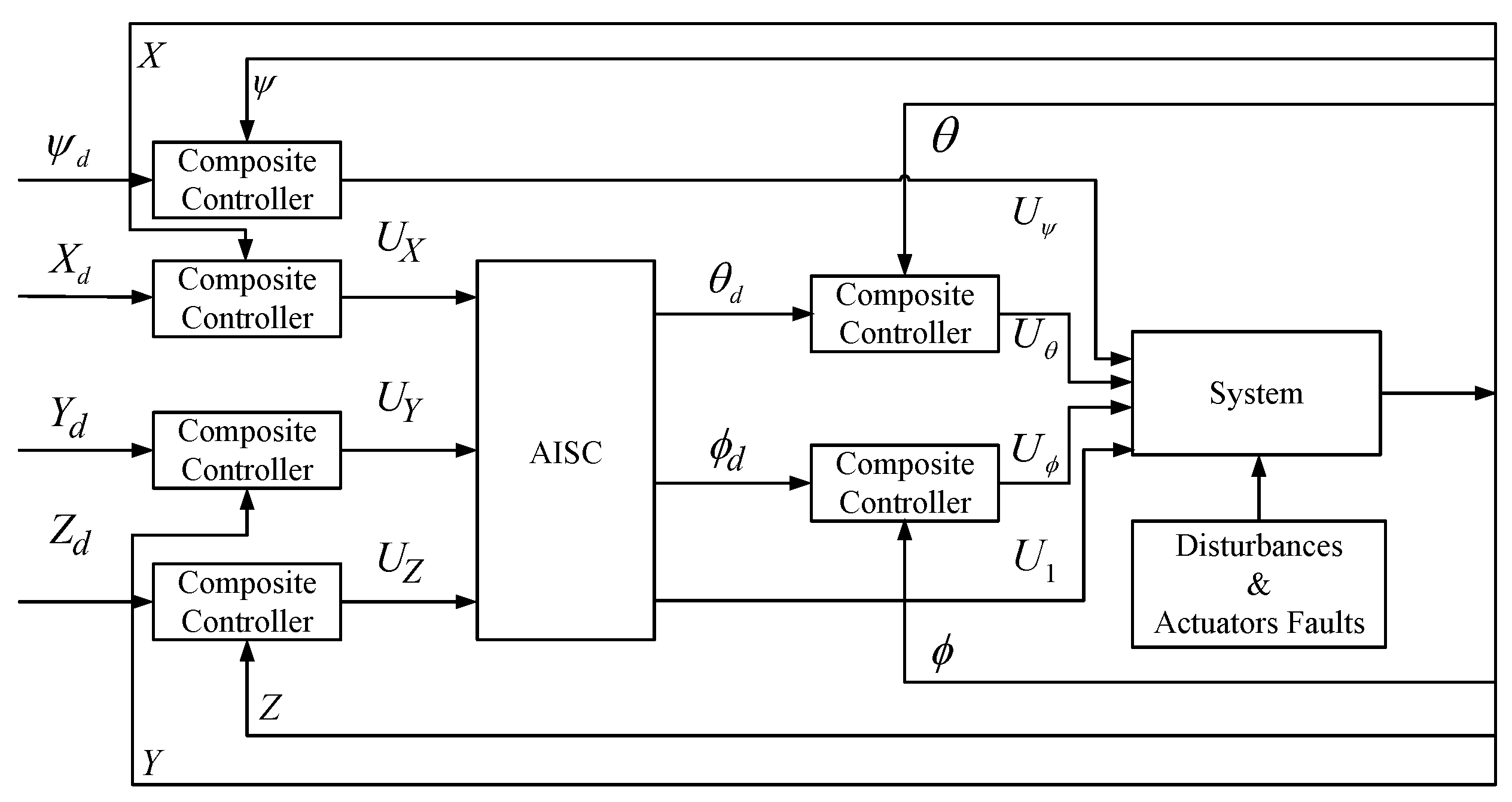
Figure 3.
The curve of the disturbance in position X channel.

Figure 4.
The curve of the disturbance in position Y channel.
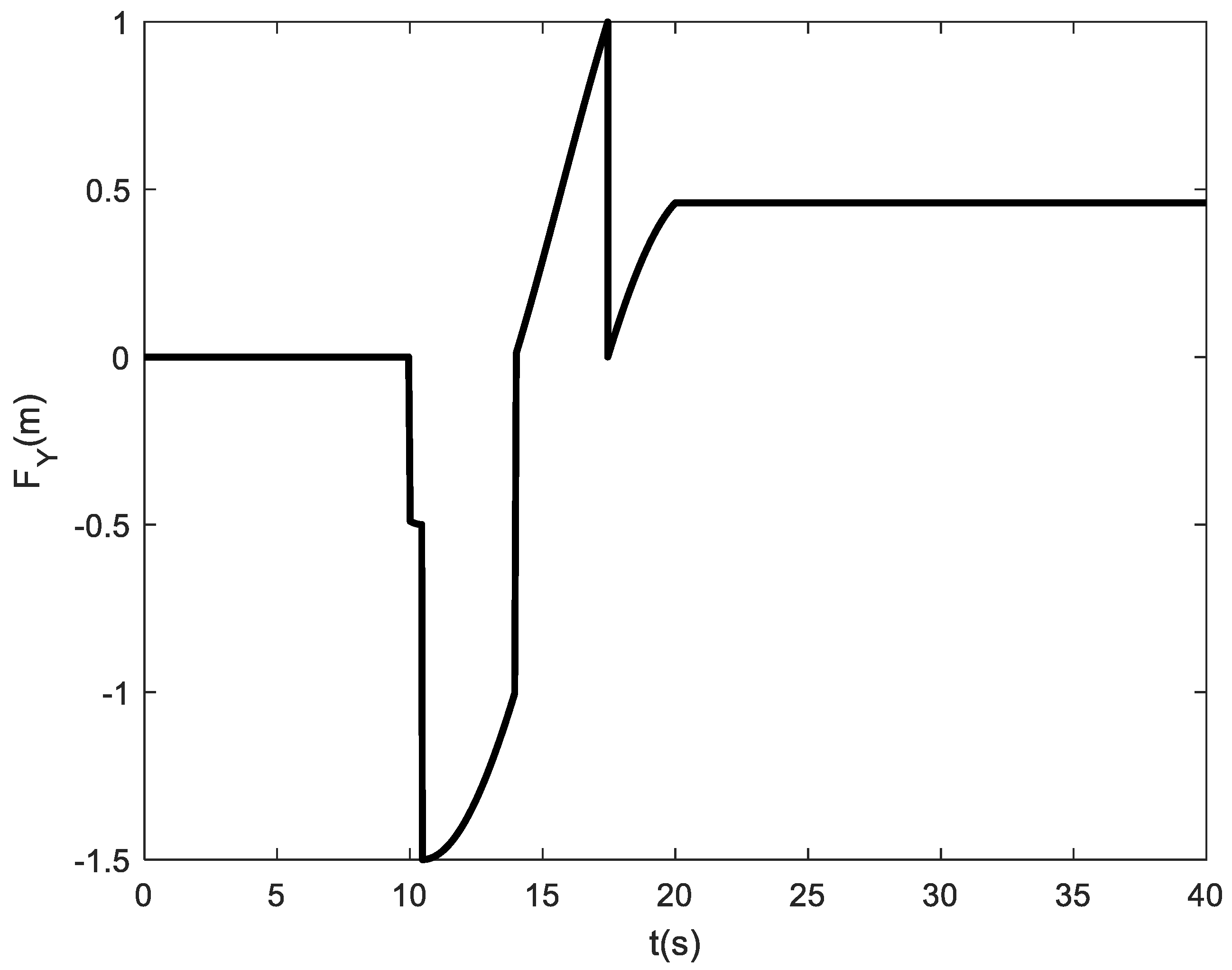
Figure 5.
The curve of the disturbance in position Z channel.
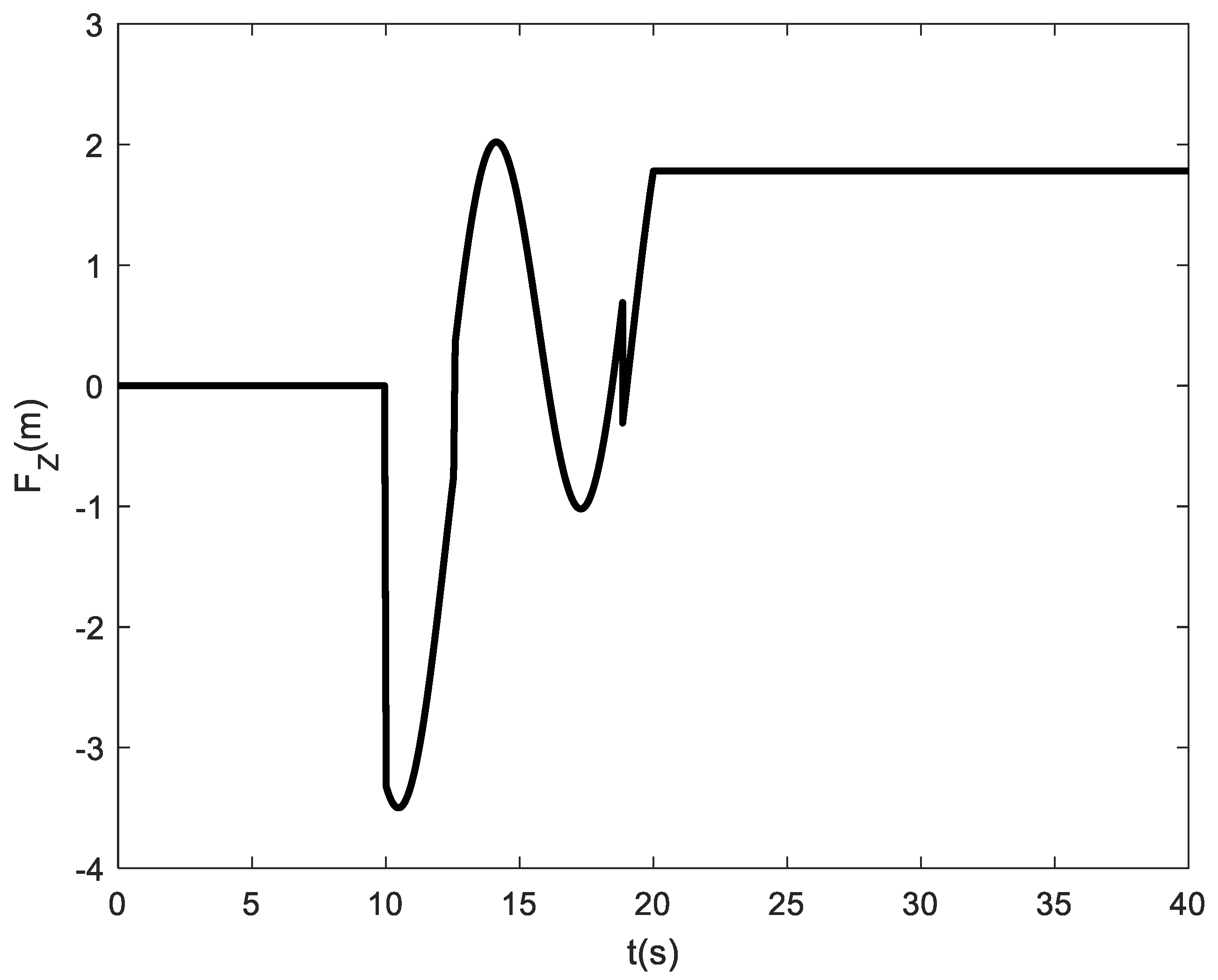
Figure 6.
The curve of the disturbance in Yaw angle channel.
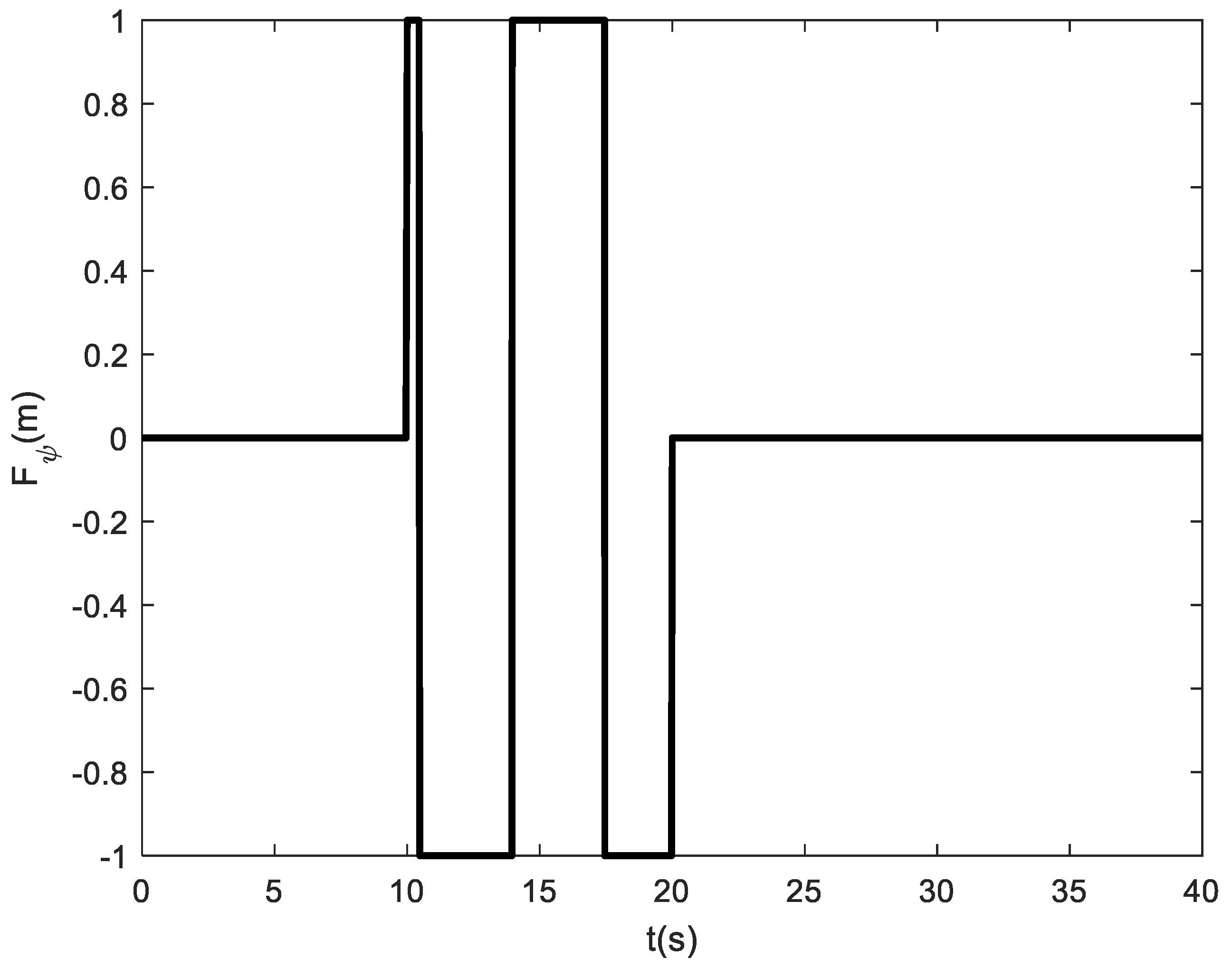
Figure 7.
The flight trajectories of the QUAV under actuator constant fault and disturbance condition.
Figure 7.
The flight trajectories of the QUAV under actuator constant fault and disturbance condition.
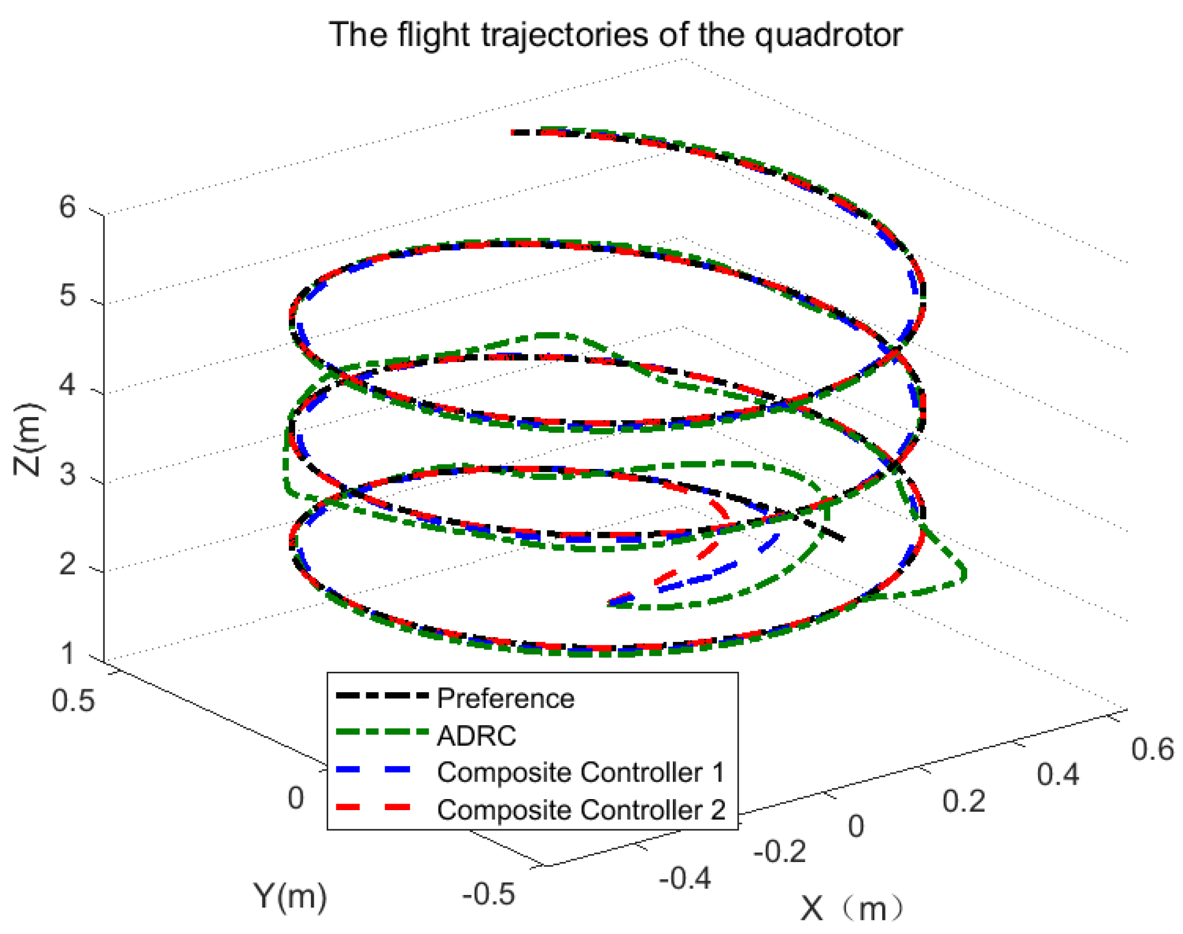
Figure 8.
Responses of position X control for QUAV under actuator constant fault and disturbance condition.
Figure 8.
Responses of position X control for QUAV under actuator constant fault and disturbance condition.
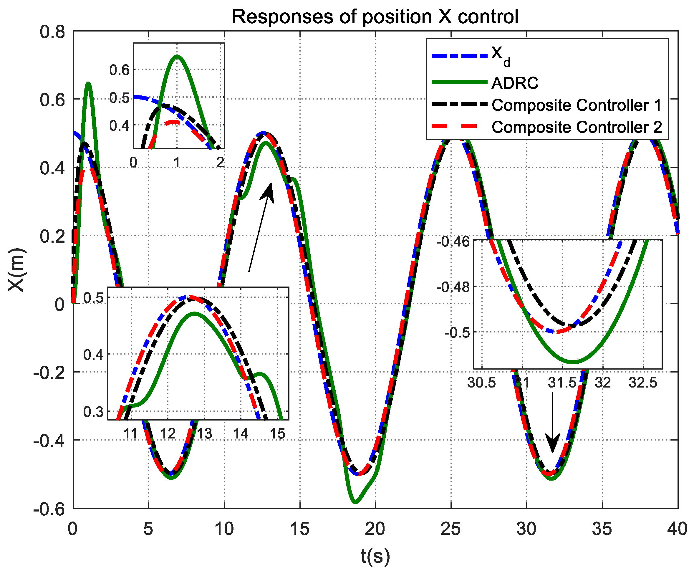
Figure 9.
Responses of position Y control for QUAV under actuator constant fault and disturbance condition.
Figure 9.
Responses of position Y control for QUAV under actuator constant fault and disturbance condition.

Figure 10.
Responses of position Z control for QUAV under actuator constant and disturbance fault condition.
Figure 10.
Responses of position Z control for QUAV under actuator constant and disturbance fault condition.

Figure 11.
Responses of Yaw angle control for QUAV under actuator constant fault and disturbance condition.
Figure 11.
Responses of Yaw angle control for QUAV under actuator constant fault and disturbance condition.
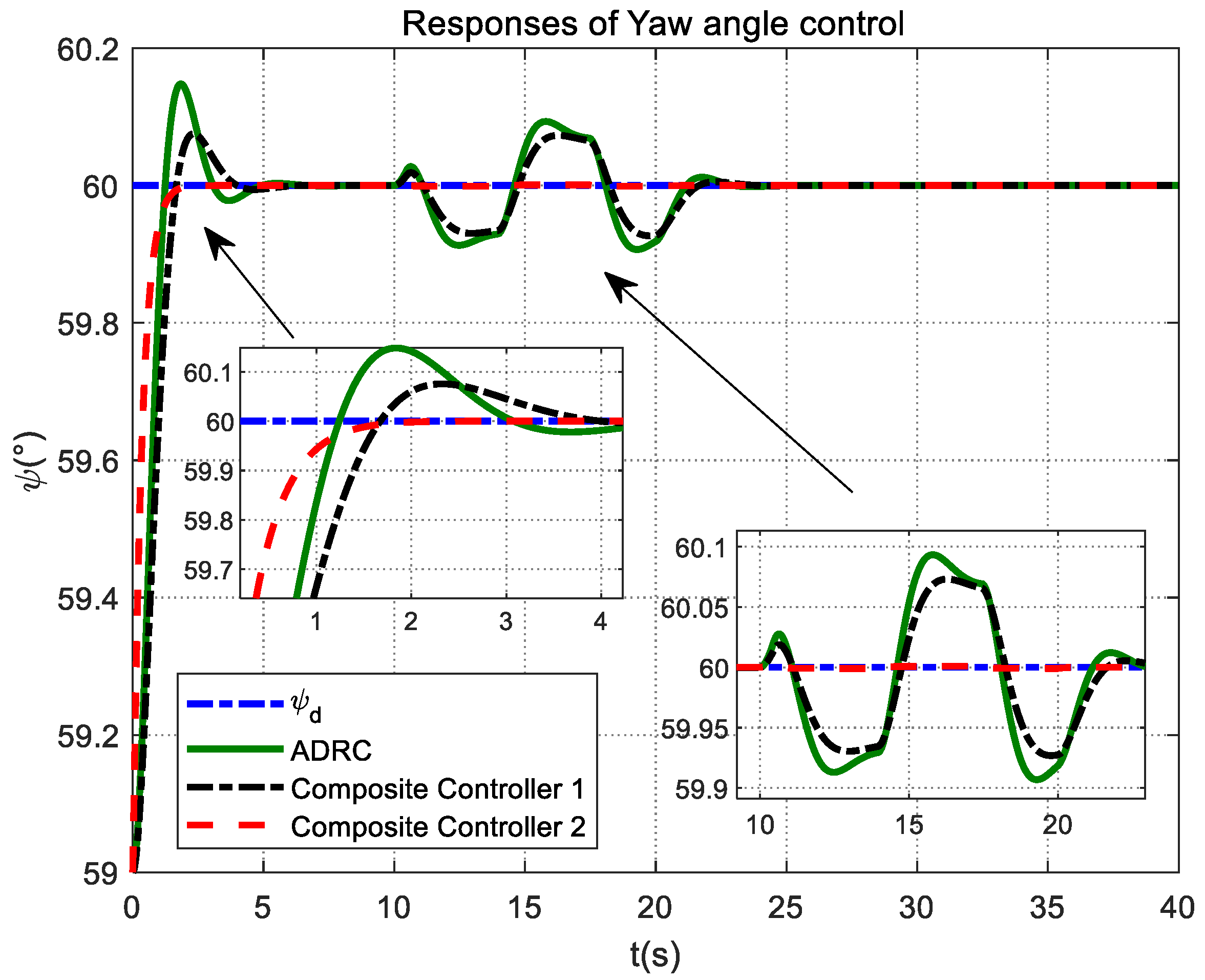
Figure 12.
Tracking error of position X control for QUAV under actuator constant fault and disturbance condition.
Figure 12.
Tracking error of position X control for QUAV under actuator constant fault and disturbance condition.
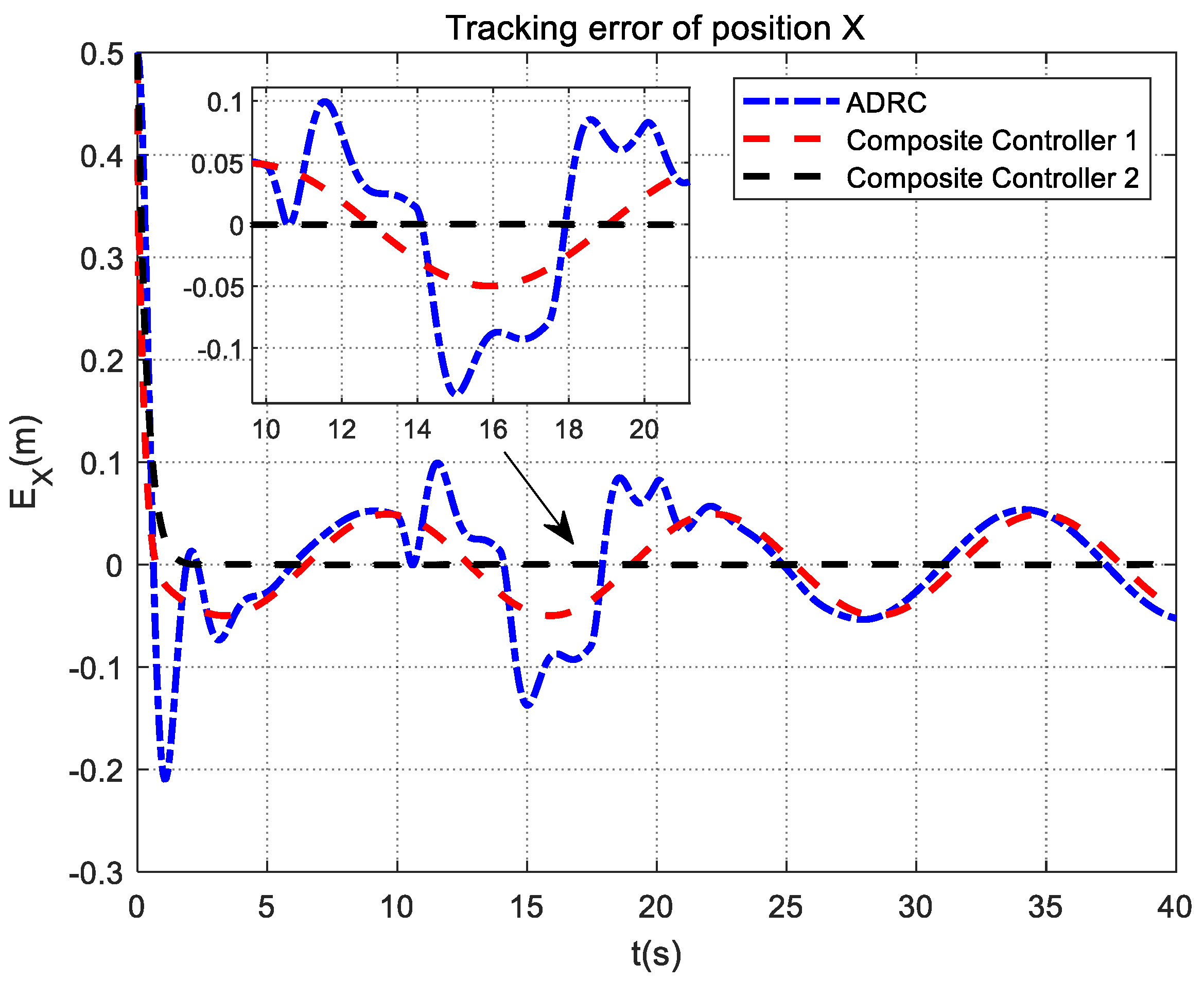
Figure 13.
Tracking error of position Y control for QUAV under actuator constant fault and disturbance condition.
Figure 13.
Tracking error of position Y control for QUAV under actuator constant fault and disturbance condition.
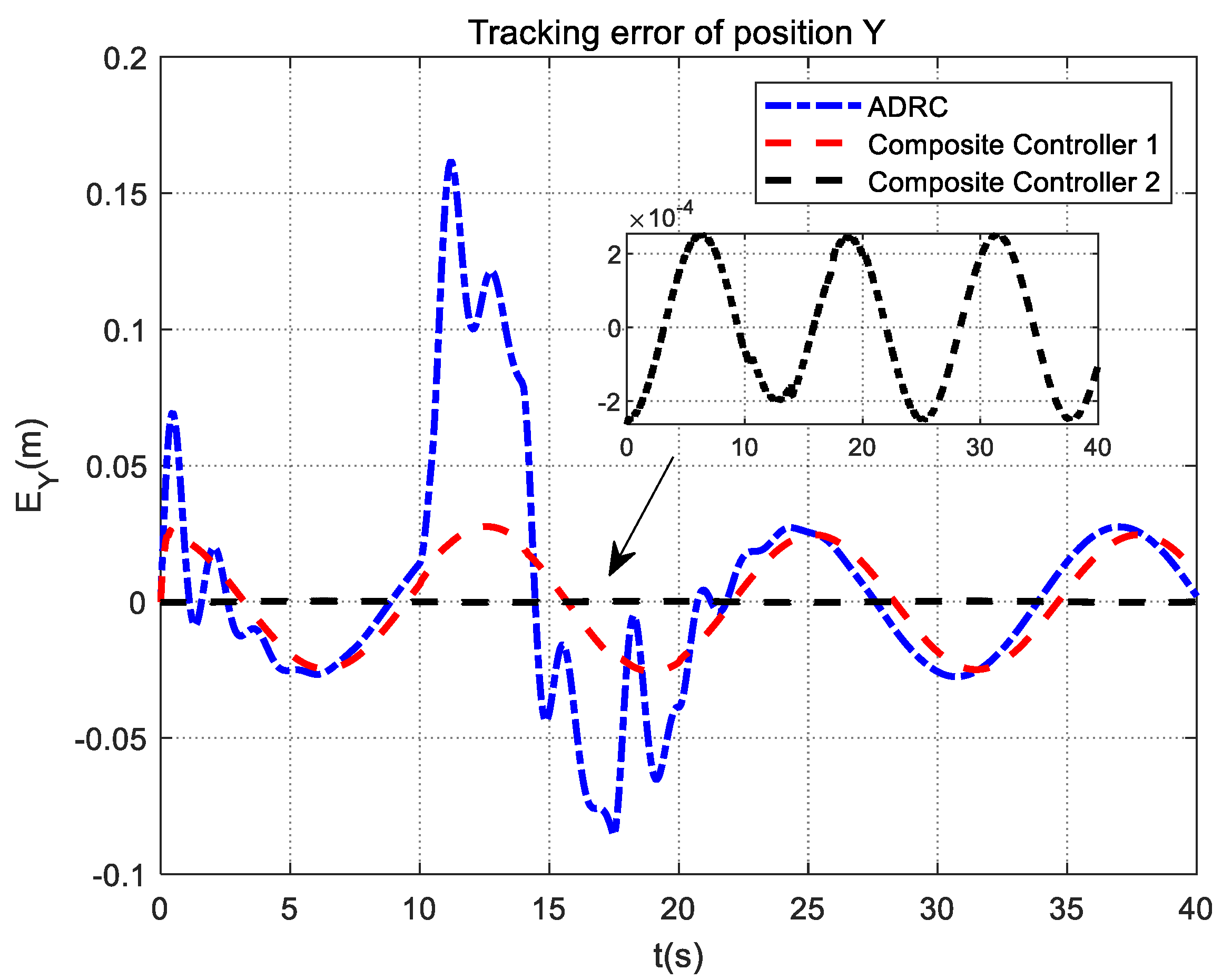
Figure 14.
Tracking error of position Z control for QUAV under actuator constant fault and disturbance condition.
Figure 14.
Tracking error of position Z control for QUAV under actuator constant fault and disturbance condition.
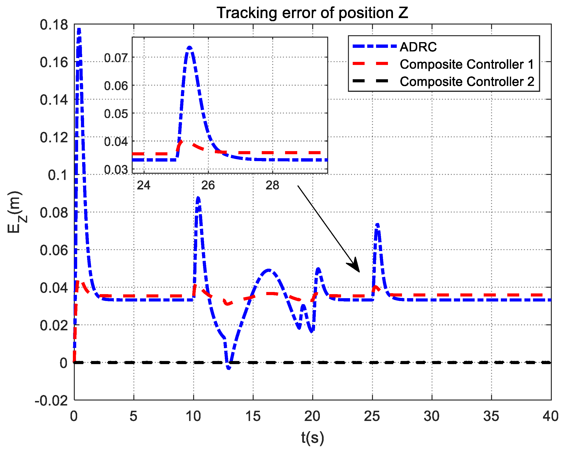
Figure 15.
Tracking error of Yaw angle control for QUAV under actuator constant fault and disturbance condition.
Figure 15.
Tracking error of Yaw angle control for QUAV under actuator constant fault and disturbance condition.

Figure 16.
The flight trajectories of the QUAV under actuator time-varying fault and disturbance condition.
Figure 16.
The flight trajectories of the QUAV under actuator time-varying fault and disturbance condition.
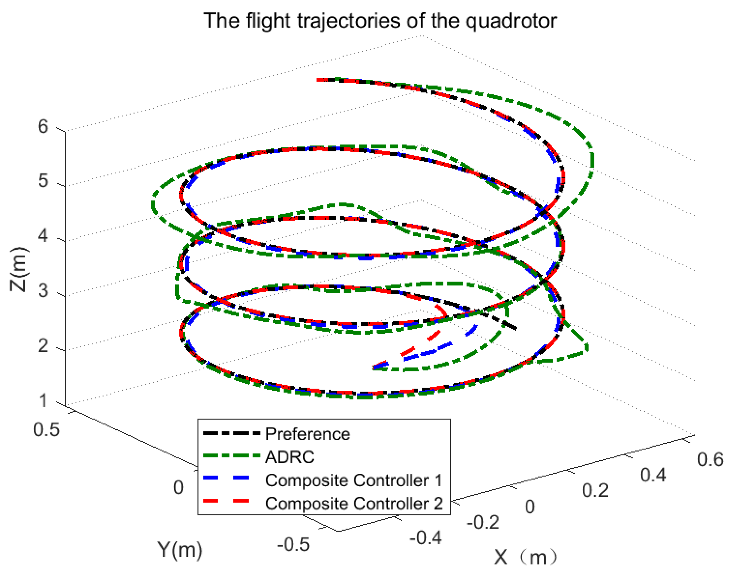
Figure 17.
Responses of position X control for QUAV under actuator time-varying fault and disturbance condition.
Figure 17.
Responses of position X control for QUAV under actuator time-varying fault and disturbance condition.
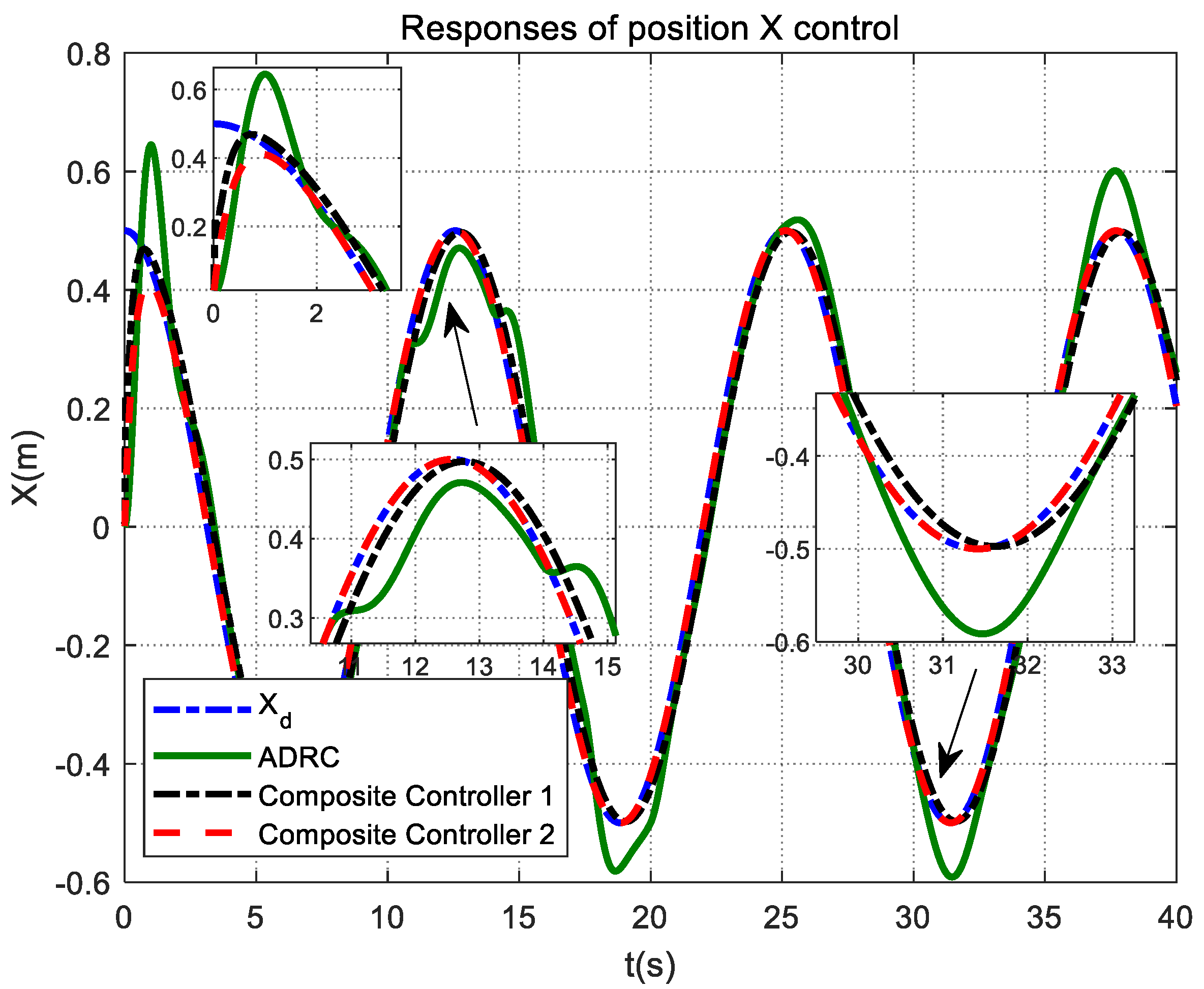
Figure 18.
Responses of position Y control for QUAV under actuator time-varying fault and disturbance condition.
Figure 18.
Responses of position Y control for QUAV under actuator time-varying fault and disturbance condition.

Figure 19.
Responses of position Z control for QUAV under actuator time-varying fault and disturbance condition.
Figure 19.
Responses of position Z control for QUAV under actuator time-varying fault and disturbance condition.
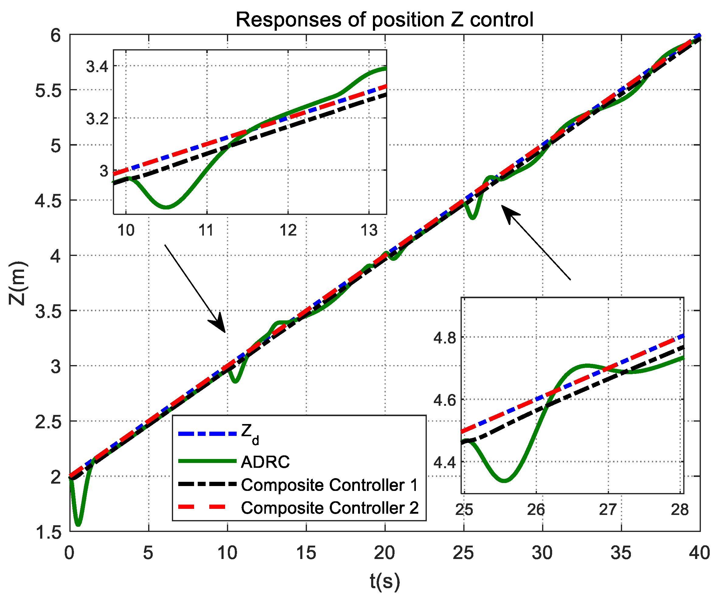
Figure 20.
Responses of Yaw angle control for QUAV under actuator time-varying fault and disturbance condition.
Figure 20.
Responses of Yaw angle control for QUAV under actuator time-varying fault and disturbance condition.
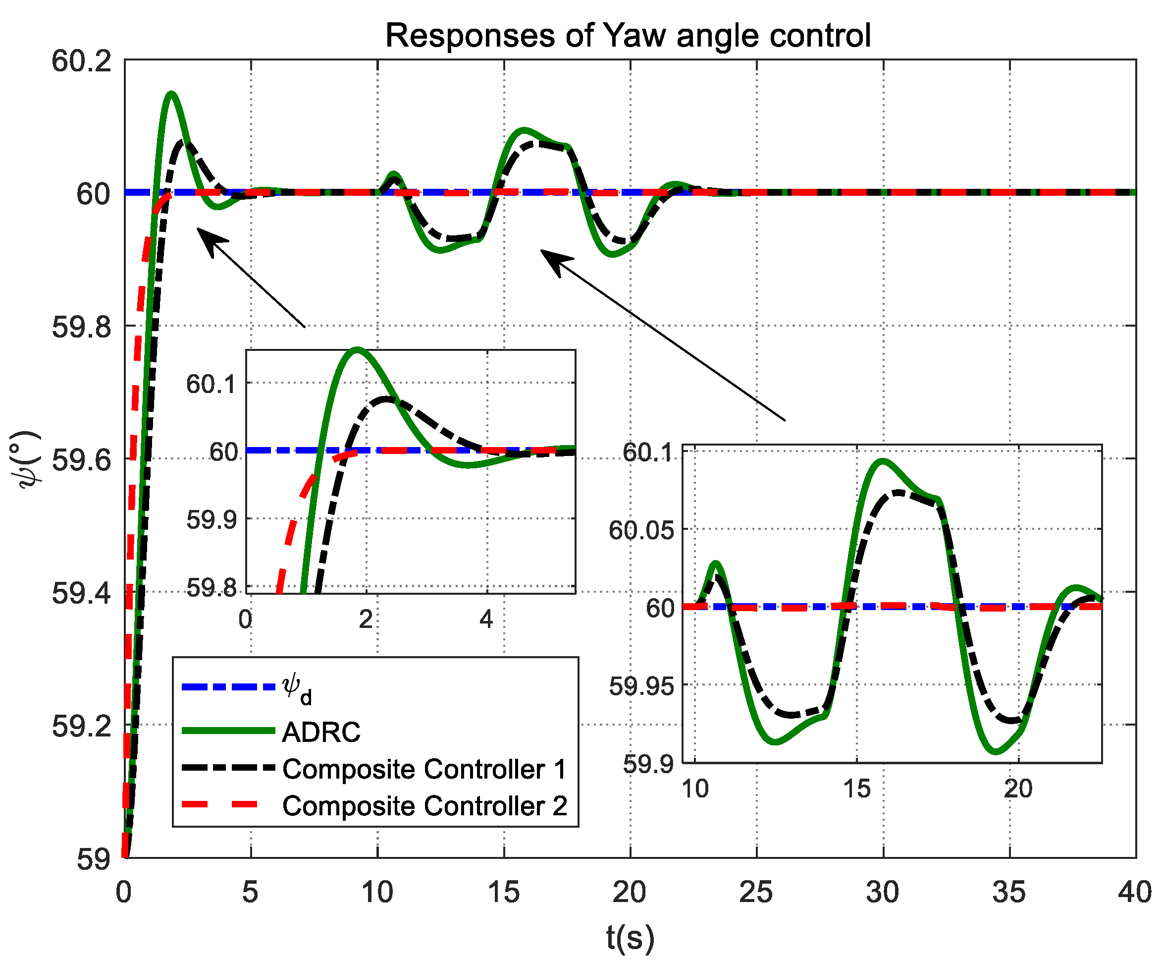
Figure 21.
Tracking error of position X control for QUAV under actuator time-varying fault and disturbance condition.
Figure 21.
Tracking error of position X control for QUAV under actuator time-varying fault and disturbance condition.

Figure 22.
Tracking error of position Y control for QUAV under actuator time-varying fault and disturbance condition.
Figure 22.
Tracking error of position Y control for QUAV under actuator time-varying fault and disturbance condition.
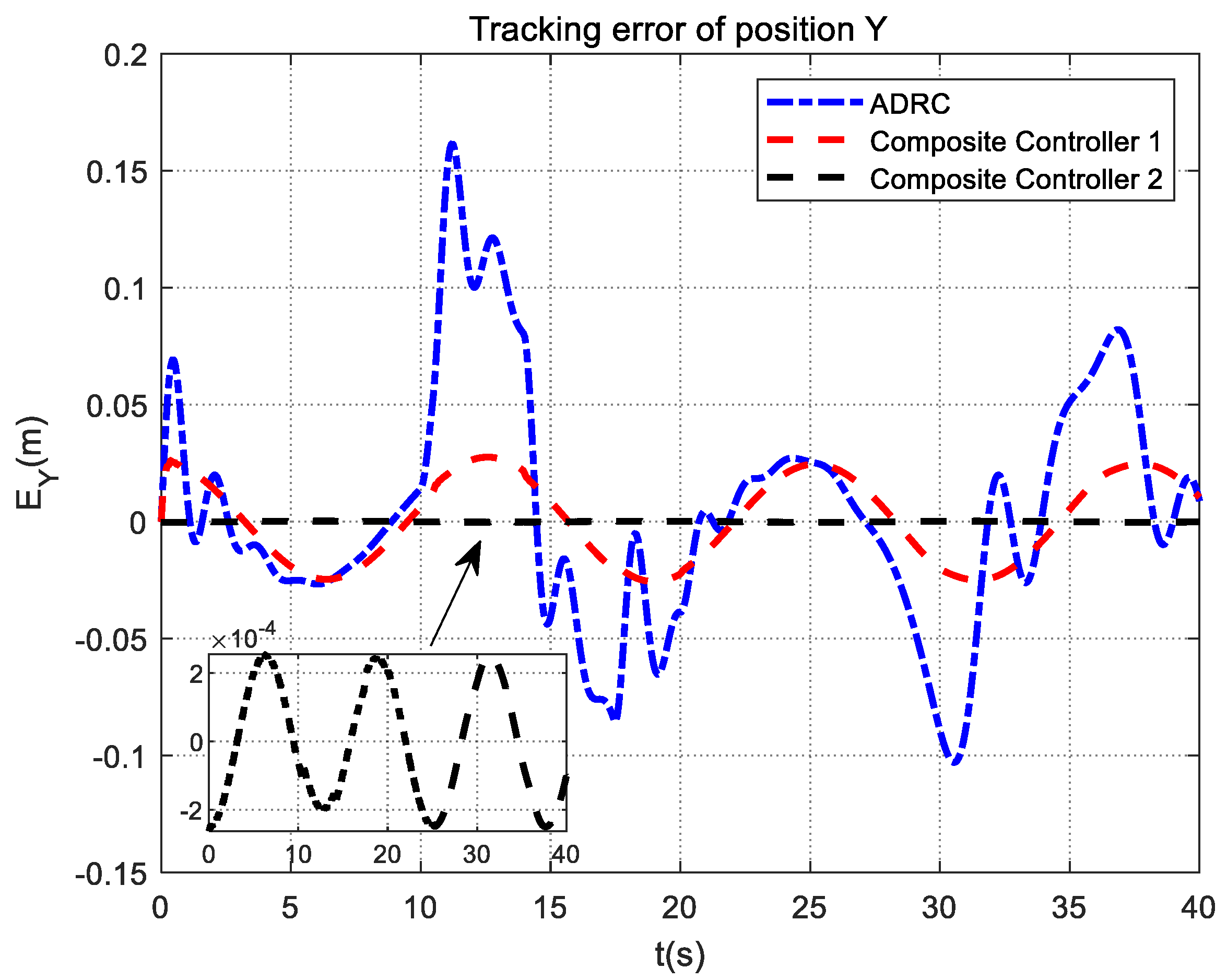
Figure 23.
Tracking error of position Z control for QUAV under actuator time-varying fault and disturbance condition.
Figure 23.
Tracking error of position Z control for QUAV under actuator time-varying fault and disturbance condition.
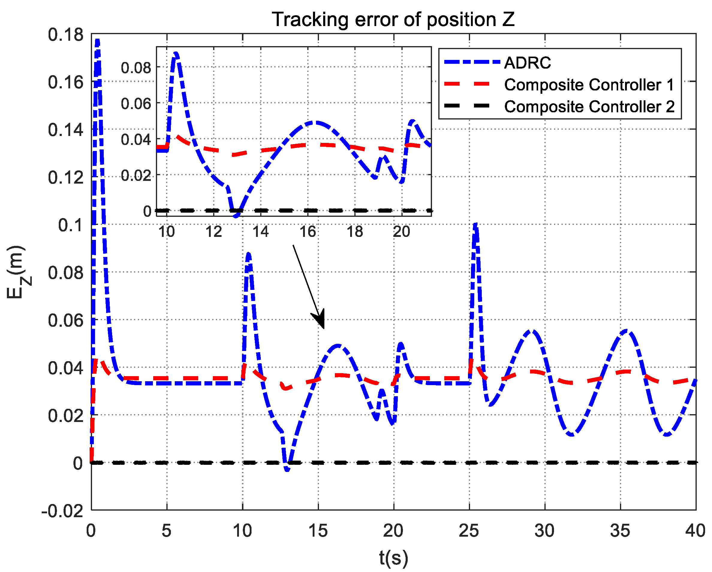
Figure 24.
Tracking error of Yaw angle control for QUAV under actuator time-varying fault and disturbance condition.
Figure 24.
Tracking error of Yaw angle control for QUAV under actuator time-varying fault and disturbance condition.


Table 1.
The values of parameters.
| Symbol | Value | Symbol | Value | Symbol | Value | Symbol | Value | Symbol | Value |
|---|---|---|---|---|---|---|---|---|---|
| 0.0552 | 0.0552 | 0.11 | 0.012 | M | 2 | ||||
| G | 9.8 | 0.8 | 3000 | 3000 | 500 | ||||
| 2500 | 125 | 100 | 0.9 | 1.2 | |||||
| 36 | 432 | 1728 | 36 | 432 | |||||
| 1728 | 0.5 | 0.09 | 0.8 | 3000 | |||||
| 3000 | 500 | 2500 | 125 | 100 | |||||
| 0.8 | 3000 | 3000 | 500 | 2500 | |||||
| 125 | 100 | 0.9 | 1.2 | 36 | |||||
| 432 | 1728 | 36 | 432 | 1728 | |||||
| 0.5 | 0.09 | 0.8 | 3000 | 3000 | |||||
| 500 | 2500 | 125 | 100 | 0.9 | |||||
| 1.2 | 36 | 432 | 1728 | 36 | |||||
| 432 | 1728 | 0.5 | 0.09 | 0.9 | |||||
| 1.2 | 36 | 432 | 1728 | 36 | |||||
| 432 | 1728 | 0.5 | 0.09 | 0.8 | |||||
| 3000 | 3000 | 500 | 2500 | 125 | |||||
| 100 | 0.9 | 1.2 | 36 | 432 | |||||
| 1728 | 36 | 432 | 1728 | 0.5 | |||||
| 0.09 | 0.8 | 3000 | 3000 | 500 | |||||
| 2500 | 125 | 100 | 0.9 | 1.2 | |||||
| 36 | 432 | 1728 | 36 | 432 | |||||
| 1728 | 0.5 | 0.09 |
Publisher’s Note: MDPI stays neutral with regard to jurisdictional claims in published maps and institutional affiliations. |
© 2022 by the authors. Licensee MDPI, Basel, Switzerland. This article is an open access article distributed under the terms and conditions of the Creative Commons Attribution (CC BY) license (https://creativecommons.org/licenses/by/4.0/).
Share and Cite
MDPI and ACS Style
Liu, L.; Liu, J.; Li, J.; Ji, Y.; Song, Y.; Xu, L.; Niu, W. Fault-Tolerant Control for Quadrotor Based on Fixed-Time ESO. Mathematics 2022, 10, 4386. https://doi.org/10.3390/math10224386
AMA Style
Liu L, Liu J, Li J, Ji Y, Song Y, Xu L, Niu W. Fault-Tolerant Control for Quadrotor Based on Fixed-Time ESO. Mathematics. 2022; 10(22):4386. https://doi.org/10.3390/math10224386
Chicago/Turabian StyleLiu, Lei, Junjie Liu, Junfang Li, Yuehui Ji, Yu Song, Liang Xu, and Wenxing Niu. 2022. "Fault-Tolerant Control for Quadrotor Based on Fixed-Time ESO" Mathematics 10, no. 22: 4386. https://doi.org/10.3390/math10224386
Note that from the first issue of 2016, this journal uses article numbers instead of page numbers. See further details here.