
A Preserving Precision Mixed Finite Element Dimensionality Reduction Method for Unsaturated Flow Problem

1
School of Digitalized Intelligence Engineering, Hunan Sany Polytechnic College, Changsha 410129, China
2
Department of Mathematics and Computer Engineering, Ordos Institute of Technology, Ordos 017000, China
*
Author to whom correspondence should be addressed.
Mathematics 2022, 10(22), 4391; https://doi.org/10.3390/math10224391
Submission received: 24 October 2022
/
Revised: 16 November 2022
/
Accepted: 18 November 2022
/
Published: 21 November 2022
(This article belongs to the Section Computational and Applied Mathematics)
Abstract
:The unsaturated flow problem is of important applied background and its mixed finite element (MFE) method can be used to simultaneously calculate both water content and flux in soil, which is the most ideal calculation method. Nonetheless, it includes many unknowns. Thereby, herein we will employ the proper orthogonal decomposition (POD) to lower the dimension of unknown solution coefficient vectors in the MFE method for the unsaturated flow problem. Thus, we first examine the MFE method for the unsaturated flow problem and the existence and convergence of the classical MFE solutions. We then take advantage of the initial L MFE solution coefficient vectors to generate a set of POD basis vectors and utilize the most POD basis vectors to create the preserving precision MFE reduced-dimension (PPMFERD) format. Under the circumstances, the PPMFERD format has the same basis functions as the classical MFE format so that it can maintain the same accuracy as the classical MFE format, but it only includes a few unknowns, so it greatly lightens the calculating load, retards the accumulation of computing errors, saves CPU runtime, and improves the accuracy of the real-time calculation in the computational process. Next, we employ the analysis of matrices to demonstrate the existence and convergence of the PPMFERD solutions such that the theoretical analysis becomes very simple and elegant. Finally, we take advantage of some numerical simulations to check on the correctness of the PPMFERD method. It shows that the PPMFERD method is effective and feasible for simulating both water content and flux in unsaturated flow soil.
1. Introduction
Previous research (see, e.g., [1,2,3]) illustrates that the governing equation of unsaturated flow problem is highly nonlinear due to the high nonlinearity of the physical behavior of unsaturated porous media. The soil water characteristic curve (SWCC) is the major reason for the nonlinear relationship of hydraulic conductivity in unsaturated soils. There are mainly two types of sigmoidal functions: unimodal and bimodal SWCCs. For convenience and without loss of generality, we herein consider the unsaturated soil water flow problem with the sigmoidal unimodal SWCC. Therefore, based on the horizontal resolution (1–5 latitude and longitude) of the atmospheric general circulation model, if the horizontal flow of soil water can be ignored, it is considered the one-dimension (1D) unsaturated soil flow problem, in which the water content has different spatial and temporal distributions. Assume that the axis of z is vertically downward, the origin of coordinates is taken as the ground, and is the soil moisture content at the point z away from the ground at time t. Moreover, suppose that the soil moisture content on the ground has a rate of infiltration or evaporation that varies over time, where infiltration is positive and evaporation is negative, but the water content distribution at the bottom varies over time. According to Darcy’s Law and continuity principle as well as previous experience, the unsaturated soil water flow problem with the sigmoidal unimodal SWCC can be summarized as the following high nonlinear partial differential equation (PDE) (see [4,5,6,7,8]).
Problem 1.
For any , find Q such that
The above is the final time, Q represents the moisture content, , is the root-water uptake rate, Z is the max soil depth, and is the soil hydraulic conductivity, is the soil water diffusivity, and , , and are, respectively, known water fluxes at the upper boundary, the water content of the lower boundary, and the water content of the initial moment.
As just mentioned in the abstract, the unsaturated flow problem has an important applied background. The prediction for the unsaturated soil water flow has great significance in atmospheric science, soil science, agricultural engineering, environmental engineering, and groundwater dynamics. As an important climatic factor, the seasonal variation of soil moisture has a great influence on the weather and climate in middle and high latitudes. The study of land surface parameterization, which mainly simulates soil water content, has become a hot topic in atmospheric science (see [4,5]). Surface and subsurface hydrological processes, such as atmospheric precipitation, evaporation and transpiration of plants, surface water leakage and updraft of deep water, root absorption, and subsurface flow, also come down to unsaturated soil water flows (see [6,7,8]).
The groundwater flow in homogeneous soil can also come down to the unsaturated soil water flow, which is a water flow when the pores in the soil are not completely filled with water. It is an important form of fluid movement in porous media. Because the above mathematical model of unsaturated soil water flow is the strong nonlinearity PDE, it is difficult to find an analytical solution except for some very special cases. Hence, the most effective method is to find its numerical solutions. The finite difference (FD) method is very sensitive to boundary conditions and soil parameters when simulating infiltration or evaporation. The standard finite element (FE) method can be used to better deal with this kind of boundary problem, but it can only be used to find the numerical solutions of soil moisture content (see [9]). The mixed FE (MFE) method in [10] can be simultaneously used to calculate both water content and flux in the soil so that it can overcome the defect of FD and FE methods. However, the MFE method also includes many unknowns so that computing errors quickly accumulate during the process of calculation to find MFE solutions, resulting in the MFE solutions having very large deviations.
Thereby, herein we mainly employ the proper orthogonal decomposition (POD) to lower the dimension of unknown solution coefficient vectors in the MFE method for the unsaturated flow problem. A lot of numerical simulating tests (see [11,12,13,14,15,16,17,18,19,20,21,22,23,24,25,26,27,28,29]) have proved that the POD method can greatly lessen the unknowns of numerical models. It has also been widely and successfully applied to various areas such as signal procedure and image recognition [30], hydrodynamics and atmospheric sciences [31], and statistics [32].
However, to our knowledge, at the moment, there is no report that the dimensionality of unknown solution coefficient vectors in the MFE method for the unsaturated soil water flow equation is reduced by using the POD technique. Therefore, herein we employ the POD method only to lower the unknown solution coefficient vectors in the MFE method but keep the basis functions unchanged so as to create a preserving precision MFE reduced-dimension (PPMFERD) format. In this case, the obtained PPMFERD format has the same basis functions as the classical MFE format so that it can keep the same accuracy as the classical MFE format, but it only has a few unknowns. Thus, the PPMFERD format can greatly lighten the calculating load, retard the accumulation of computing errors, save CPU runtime, and improve the accuracy of the real-time calculation in the computational process.
Although the reduced-dimensional methods of the unknown FE solution coefficient vectors for the hyperbolic, parabolic, Sobolev, viscoelastic wave, and unsteady Stokes equations, together with fractional diffusion equation have been posed in [24,25,26,27,28], respectively, the MFE method including both water content and flux for the unsaturated flow problem herein is more complicated than the FE methods for the above six types of equations, thereby creating the PPMFERD method and the discussing the existence and convergence to the PPMFERD solutions have more difficulties and require more skills [24,25,26,27,28]. However, the PPMFERD method including both water content and flux in soil for the unsaturated flow problem has a wide range of uses. Therefore, herein it is of great significance to study the reduced dimensions of unknown solution coefficient vectors in the MFE method for the unsaturated flow problem by means of the POD method. Hence, the study herein is very valuable.
For this purpose, we first examine the MFE method for the unsaturated flow problem and the existence and convergence of the classical MFE solutions in Section 2. We then take advantage of the initial L MFE solution coefficient vectors to generate a set of POD basis vectors and utilize the few most POD basis vectors to establish the PPMFERD model and employ the analysis of matrices to demonstrate the existence and convergence of the PPMFERD solutions in Section 3. Next, we utilize some numerical simulations to check on the effectiveness of the PPMFERD method in Section 4. Afterward, in Section 5, we provide some discussions. Finally, we will summarize the main conclusions of this article in Section 6.
2. The Classical MFE Method for the Unsaturated Flow Problem
2.1. The Functional Form of MFE Format for the Unsaturated Flow Problem
There holds the following relationships between the above soil hydraulic conductivity and soil water diffusivity D with the moisture content Q in Problem 1.
where () and represent the saturated water content and residual water content in the soil, respectively, and the saturated water conductivity , soil parameters b, and saturated soil water potential are known constants. Obviously, , , , and are bounded, namely there exist two constants and such that
In order to establish the classical MFE method, we need to introduce the following moisture flux function
which plays an important role in the study of land surface processes. With this splitting, the water content in the soil and the water flux through the soil can be calculated simultaneously. In order to homogenize the boundary conditions, we need further to introduce the following intermediate variables
Since varies very little with respect to t, we may assume that . Thus, by using (7) and (8), Problem 1 can be rewritten as follows.
Problem 2.
For any , find such that
Let , represent the square Lebesgue integrable space on with inner product , and represent the familiar Sobolev space. If we set that , , , , and , then the mixed variational form for Problem 2 can be built as follows.
Problem 3.
For any , find such that
The following conclusion of the existence and uniqueness as well as stability of the mixed generalized solutions for Problem 3 has been proved in [10].
Theorem 1.
If and , and and , then Problem 3 exists a unique set of solutions , and there exist two constants and such that
In order to establish the MFE format, we need to employ the FD method to discretize the time for Problem 3 and use the FE method to discretize the spatial variable for Problem 3. Thereupon, we assume that N is the positive integer, represents the time-step increment, and is the regular subdivision on , namely
satisfies that there exists the positive constant such that . If we assume that is the space formed by linear polynomials defined on , we can define the following MFE subspaces
If we assume that are the MFE approximations for at , then the MFE solutions for Problem 3 are stated as follows.
Problem 4.
Find such that
The following conclusion of the existence and error estimates for the MFE solutions to Problem 4 has been proved in [10].
Theorem 2.
Under the conditions of Theorem 1, when is sufficiently small, Problem 4 has a unique set of solutions satisfying the following error estimates
The above are the state of to Problem 2 at and c used in context is the constant independent of and h.
2.2. The Matrix Representation of MFE Format for the Unsaturated Flow Problem
Without loss of generality, we might as well take . Let be the length of . Then, the basis functions of linear interpolation on each element in both and formed by the piecewise linear functions can be denoted by
On each element , let
and
Then, on each element , the stiffness matrix and unknown vector, as well as the right end term for Problem 4, can be expressed as follows:
In order to synthesize the total equation, the FE stiffness matrix and unknown vector are appropriately transformed into the following
By using the whole synthesis technology of the FE method, the system of Equation (15), i.e., Problem 4, can be expressed as the following matrix form.
Problem 5.
Find and such that
Thereinto
After obtaining and from (21), the MFE solutions to Problem 1 can be found as follows:
Thus, as long as the spatial step , time step , initial boundary value, and values of parameters , b, and are given, by solving the system of Equations (21) and (22), we can obtain the MFE solutions to Problem 1, namely the MFE solutions of water content and flux.
Remark 1.
If the original problem, i.e., Problem 1, is the first boundary value condition, namely if the water content on the left boundary is also given, it is only necessary to change the homogeneous boundary conditions a little bit, namely to get rid of q in and add appropriately large numbers to the elements in the first row and column (upper left corner) in the coefficient matrix in (21) such that on the right side can satisfy the left boundary value condition and the first row and column form a block diagonal matrix with the rest of the elements.
3. The PPMFERD Method for the Unsaturated Flow Problem
3.1. Structure of POD Basis Vectors
In order to establish the PPMFERD format, we first solve the system of Equation (21) at the initial L steps to get the MFE solution coefficient vectors , ,…, and combine the snapshot matrix , ,…, . We then calculate the the positive eigenvalues rank of and the corresponding orthogonalized eigenvectors . We finally obtain a set of POD basis vectors () with from the foremost d vectors in . If we assume that and is the Euclidean norm to the vector , then there holds the following equality (see [11]):
If we assume that are the Lth-dimension orthonormal vectors with only nth component 1, from (23) we deduce the following estimates:
3.2. The Creation of PPMFERD Format for the Unsaturated Flow Problem
If we assume that , ; , ; and , we may obtain the initial L PPMFERD solutions () from (24). Replacing the vectors in Problem 5 with , we can create the PPMFERD format as follows.
Problem 6.
Seek and that satisfy
The above () are the initial L solution vectors for Problem 5 and are the same as those for Problem 5.
Remark 2.
Owing to the invertibility for the matrix , namely the unique solvability for Problem 4, Problem 6 has a unique set of PPMFERD solutions . It is worth noting that Problem 6 at every time node only contains unknowns , whereas Problem 4 has unknowns at the same time node, but both have the same FE basis functions and the same accuracy. Hence, Problem 6 visibly advantages over Problem 5, i.e., Problem 4, which means that Problem 6 could not only immensely lessen the unknowns, but could also vastly lessen the CPU runtime, retard the accumulation of computing errors, and improve the accuracy of the real-time calculation of numerical solutions.
3.3. The Error Analysis of PPMFERD Solutions
The unsaturated soil property is one of the key factors affecting the accuracy of the numerical methods. Therefore, for ease of application, in land surface and atmospheric circulation models, Dickinson et al. classified the properties of global unsaturated soils into some typical categories (see [4]), as shown in Table 1.
From Table 1 and the definitions D and and by the estimate of banded matrices, we can deduce that in (5) and the norm of the matrix satisfies that
When , noting that and , by (24) and Theorem 2 we get
When , the second equation in the system of Equation (25) can be rewritten as follows
By the first equation in the system of Equation (5), we get
By the construction of we get
Thus, we get
Theorem 3.
Under the conditions of Theorems 1 and 2, the solutions satisfy the following error estimates
Thereinto, is the state of in Problem 2 at .
Remark 3.
Compared with Theorem 2, the errors of Theorem 3 increase one term, , which is brought by the reduced dimension for Problem 4 and may serve as the suggestion to elect the number d of POD basis vectors. Nonetheless, if only the selecting number d of POD basis vectors satisfies , it would not make any difference to the total errors. Many numerical simulations (see, e.g., [11,12,13,14,15,16,17,18,19,20,21,22,23,24,25,26,27,28]) have shown that the eigenvalues could rapidly decrease into zero. Generally, while or 6, the factor is already very tiny and meets . What is more, if the PPMFERD solution from Problem 6 at cannot reach the desired accuracy, but at still meets the required accuracy, then we may extract a set of new vectors to generate a set of new POD basis vectors and create the new PPMFERD format so as to be able to calculate the PPMFERD solutions meeting the required accuracy. This is incomparable to the classical MFE format, namely Problem 4.
4. Some Numerical Simulations for the Unsaturated Flow Problem
Taking the eighth soil parameter in Table 1 as an example and comparing the numerical simulating results of the MFE format with the PPMFERD format, we see that water infiltration and evaporation occur successively in the unsaturated soils problem exhibit the advantage of the PPMFERD format.
The eighth soil parameters imply that mm, mm/s, , and . If taking cm and the spatial step cm, we cut into equal small intervals. Moreover, we take h and the time step h. Further, the constant infiltration flux is assumed to be maintained at the soil surface () for a period of time, the boundary values and , and the initial and boundary conditions of soil water infiltration and evaporation are as follows:
Thus, according to Theorems 2 and 3, the theoretical errors should reach .
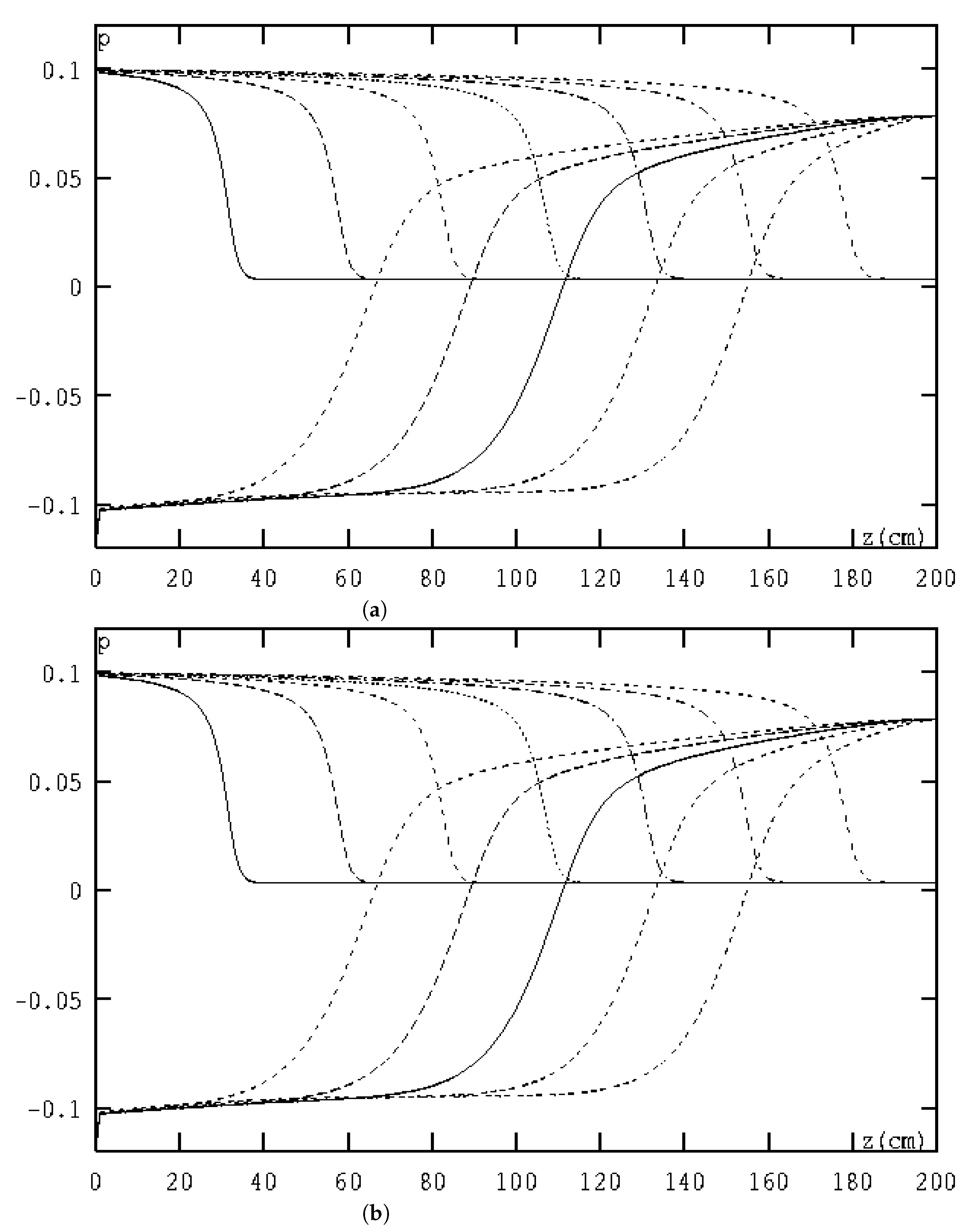
When , we enter the data into the system of Equation (21) of the MFE method and calculate the first 20 sets of solution coefficient vectors , ,..., and combine the snapshot matrix , ,…, . We then calculate the the positive eigenvalues of the matrix . By estimating we obtain that , so we need only to take the first six orthonormal eigenvectors of to generate a set of POD basis vectors with . We input into Problem 6 to calculate the PPMFERD solutions of infiltration of water content and flux in the soil at h, 60 h,…, 420 h, and present Figure 1a and Figure 2a, where each of curves represents the PPMFERD solutions of infiltration of water content and flux in the soil that are outputted once every 30 h. We also calculate the PPMFERD solutions of infiltration and evaporation of water content and flux in the soil at h, 120 h,…, 420 h, 480 h,…, 840 h and present Figure 3a and Figure 4a, where each of curves represents the PPMFERD solutions of infiltration and evaporation of water content and flux in the soil that are outputted once every 60 h, and the water content and flux from 0 to 420 h are the infiltration case, but the water content and flux after 420 h are the evaporation case.
For comparison, we also calculate the classical MFE solutions of water content and flux in the soil at h, 60 h,…, 420 h and present Figure 1b and Figure 2b, where each of curves represents the MFE solutions of infiltration of water content and flux in the soil that are outputted once every 30 h. We also calculate the classical MFE solutions of water content and flux in the soil at h, 120 h,…, 420 h, 480 h,…, and 840 h and present Figure 3b and Figure 4b, where each of curves represents the MFE solutions of infiltration and evaporation of water content and flux in the soil that are outputted once every 60 h, and the water content and flux from 0 to 420 h are also the infiltration case, but the water content and flux after 420 h are also the evaporation case.
Comparing each pair of photographs in Figure 1, Figure 2, Figure 3 and Figure 4 shows that the figures of PPMFERD solutions are highly similar to the figures of classical MFE solutions since both the PPMFERD method and the classical MFE method have the same FE basis function so as to preserve the same accuracy. Both the numerical simulating errors also reach , which is according to the theoretical errors. However, the PPMFERD format has only twelve unknowns at every time step, whereas the classical MFE format has forty thousand unknowns at the same time step. Therefore, the CPU runtime for the classical MFE method is far more than that for the PPMFERD method. For instance, calculating the PPMFERD solutions at h by the PPMFERD method needs only about 121 s on an Hp-i5-laptop by means of MATLAB software, but calculating the classical MFE solutions at h by the classical MFE method needs about 8926 s on the same laptop by means of MATLAB software. Moreover, finding the PPMFERD solutions at h with the PPMFERD format spends only about 240 s on the same Hp-i5-laptop by means of MATLAB software, but seeking the classical MFE solutions at h with the classical MFE format needs about 17,860 s on the same laptop by means of MATLAB software. For more details, see Table 2.
In Table 2, the errors for the MFE solutions and the PPMFERD solutions are approximately calculated by and , respectively, which are the accumulation of errors over the entire time domain.
The data in Table 2 have also shown that as the time nodes go forward, the CPU runtime for the classical MFE method (having 40,000 unknowns at each time node) increases rapidly, but the CPU runtime for the PPMFERD method (only having 12 unknowns at the same time node) increases very slowly. When h, the CPU runtime for the classical MFE method is about 87 times that of the PPMFERD method, in other words, the PPMFERD method can greatly save the CPU runtime. Owing to the accumulation of computing errors, the errors of the classical MFE solutions gradually increase and exceed the theoretical error when , but the errors of the PPMFERD solutions increase slowly and always stay within the range of the theoretical error . It is further shown that the PPMFERD method is far better than the classical MFE method and is very effective for solving the unsaturated flow problem.
5. Discussions
We have proved theoretically that the PPMFERD method has optimal order convergence and have employed some numerical simulations to verify the correctness of theoretical results. From the above numerical simulations, we have seen that when the PPMFERD method is used to solve for the unsaturated flow problem, it can greatly lessen the unknowns and improve the computational efficiency.
Although herein we have only studied the PPMFERD method for the 1D unsaturated flow problem, the approach can be generalized to 2D and 3D unsaturated flow problems or more complex real-world engineering problems.
In fact, the numerical computations in all scientific engineering, not limited to the numerical methods for the unsteady PDEs, need to be changed into the large-scale iterative algorithms, which can be reduced by means of the reduced-dimension method in Section 3.
For instance, linear or nonlinear programming problems with constraint conditions, machine learning or deep learning, data assimilation, etc., eventually have to be transformed into large-scale linear or nonlinear algebra equations to be solved iteratively. They all can be expressed in the following matrix equations
Thereinto, are very high-dimension unknown vectors, which can reach millions or even tens of millions of dimensions.
Thus, according to the reduced-dimension method in Section 3, we may first compute L steps solutions (empirical value ) and combine them into the snapshot matrix , which are also formed with the observation values of experiments. We then may employ the POD method in Section 3 to generate the POD basis vectors , which are the eigenvectors corresponding to the main eigenvalues of such that is not more than the required accuracy.
Let and be the d-dimensional unknown vectors. Substituting in the above large-scale linear or nonlinear algebra Equation (35) with , we obtain the following reduced-dimension equations that only include few d unknowns:
Thereinto, are known or the observation values from experiments.
If the reduced-dimension Equation (36) is linear, it can be directly solved iteratively; if the reduced-dimension Equation (36) is nonlinear, it can be solved by the Newton method or other methods of nonlinear algebra equations. Hence, the PPMFERD method has very comprehensive applications.
The future work on the PPMFERD method is to lower the dimensionality of the numerical computations in scientific engineering, including the MFE methods for the 2D and 3D unsaturated flow problems.
6. Conclusions and Discussions
Herein, we have studied the reduced dimension of the unknown solution coefficient vectors in the MFE method including both water content and flux in soil for the unsaturated flow problem. We have not only created the PPMFERD method for the unsaturated flow problem by means of the POD technique but also analyzed the existence and convergence (errors) of the PPMFERD solutions by using the matrix analysis in detail, even reasonably using some numerical simulations to check on the effectiveness of the PPMFERD method. The dimensionality of the PPMFERD method is far less than that of the classical MFE method, so that it can not only greatly retard the accumulation of computing errors and lighten the calculating load, but can also immensely save CPU running time. What is important, the reduced dimension for the unknown MFE solution coefficient vectors in the MEF format including both water content and flux in soil for the unsaturated flow problem is proposed for the first time, both theory and method are new and differ considerably from all previous reduced-order methods.
Author Contributions
Z.L. and Y.L. contributed to the draft of the manuscript. All authors have read and agreed to the published version of the manuscript.
Funding
This research was supported by Ordos Science and Technology Plan Project (2022YY041), Inner Mongolia Natural Science Foundation (2019MS06013), and National Natural Science Foundation of China (11671106).
Institutional Review Board Statement
Not applicable.
Informed Consent Statement
Not applicable.
Data Availability Statement
Not applicable.
Conflicts of Interest
The authors declare no conflict of interest.
References
- Rahimi, A.; Rahardjo, H.; Leong, E. Effect of range of soil-water characteristic curve measurements on estimation of permeability function. Eng. Geol. 2015, 185, 96–104. [Google Scholar] [CrossRef]
- Li, Y.; Vanapalli, S.K. Models for predicting the soil-water characteristic curves for coarse and fine-grained soils. J. Hydrol. 2022, 612, 128248. [Google Scholar] [CrossRef]
- Yoon, S.; Chang, S.; Park, D. Investigation of soil-water characteristic curves for compacted bentonite considering dry density. Prog. Nucl. Energ. 2022, 151, 104318. [Google Scholar] [CrossRef]
- Dai, Y.J.; Zeng, Q.C. A land surface model (IAP94) for climate studies, Part I: Formulation and validation in off-line experiments. Adv. Atmos. Sci. 1997, 14, 433–460. [Google Scholar]
- Ye, D.Z.; Zeng, Q.C.; Guo, Y.F. Contemporary Climatic Research; Climatic Press: Beijing, China, 1991. (in Chinese) [Google Scholar]
- Bear, J. Dynamics of Fluids in Porous Media; American Elsevier Publishing Company: New York, NY, USA, 1972. [Google Scholar]
- Lei, Z.D.; Yang, S.X.; Xie, S.C. Soil Hydrodynamics; Tsinghua University Press: Beijing, China, 1988. (in Chinese) [Google Scholar]
- Xie, Z.H.; Zeng, Q.C.; Dai, Y.J.; Wang, B. Numerical simulation of an unsaturated flow equation. Sci. China Ser. D 1998, 41, 429–436. [Google Scholar] [CrossRef]
- Xie, Z.H.; Zeng, Q.C.; Dai, Y.J.; Wang, B. Application of finite element method to unsaturated soil flow problem. Climate Environ. Res. 1998, 28, 73–81. [Google Scholar]
- Luo, Z.D.; Xie, Z.H.; Zhu, J.; Zeng, Q.C. Mixed finite element method and numerical simulation for the unsaturated soil water flow problem. Math. Numer. Sin. 2003, 25, 113–128. [Google Scholar]
- Luo, Z.D.; Chen, G. Proper Orthogonal Decomposition Methods for Partial Differential Equations; Academic Press of Elsevier: San Diego, CA, USA, 2018. [Google Scholar]
- Alekseev, A.K.; Bistrian, D.A.; Bondarev, A.E.; Navon, I.M. On linear and nonlinear aspects of dynamic mode decomposition. Int. J. Numer. Meth. Fluids 2016, 82, 348–371. [Google Scholar] [CrossRef]
- Du, J.; Navon, I.M.; Zhu, J.; Fang, F.; Alekseev, A.K. Reduced order modeling based on POD of a parabolized Navier-Stokes equations model II Trust region POD 4D VAR data assimilation. Comput. Math. Appl. 2013, 65, 380–394. [Google Scholar] [CrossRef]
- Li, H.R.; Song, Z.Y. A reduced-order energy-stability-preserving finite difference iterative scheme based on POD for the Allen-Cahn equation. J. Math. Anal. Appl. 2020, 491, 124245. [Google Scholar] [CrossRef]
- Li, H.R.; Song, Z.Y. A reduced-order finite element method based on proper orthogonal decomposition for the Allen-Cahn model. J. Math. Anal. Appl. 2021, 500, 125103. [Google Scholar] [CrossRef]
- Song, Z.Y.; Li, H.R. Numerical simulation of the temperature field of the stadium building foundation in frozen areas based on the finite element method and proper orthogonal decomposition technique. Math. Method Appl. Sci. 2021, 44, 8528–8542. [Google Scholar] [CrossRef]
- Zhu, S.; Dede, L.; Quarteroni, A. Isogeometric analysis and proper orthogonal decomposition for parabolic problems. Numer. Math. 2017, 135, 333–370. [Google Scholar] [CrossRef]
- Kunisch, K.; Volkwein, S. Galerkin proper orthogonal decomposition methods for a general equation in fluid dynamischs. SIAM J. Numer. Anal. 2002, 40, 492–515. [Google Scholar] [CrossRef]
- Li, K.; Huang, T.Z.; Li, L.; Lanteri, S.; Xu, L.; Li, B. A Reduced-Order Discontinuous Galerkin Method Based on POD for Electromagnetic Simulation. IEEE Trans. Antennas Propag. 2018, 66, 242–254. [Google Scholar] [CrossRef]
- Hinze, M.; Kunkel, M. Residual based sampling in POD model order reduction of drift-diffusion equations in parametrized electrical networks. J. Appl. Math. Mech. 2012, 92, 91–104. [Google Scholar] [CrossRef] [Green Version]
- Stefanescu, R.; Navon, I.M. POD/DEIM nonlinear model order reduction of an ADI implicit shallow water equations model. J. Comput. Phys. 2013, 237, 95–114. [Google Scholar] [CrossRef] [Green Version]
- Zokagoa, J.M.; Soulaǐmani, A. A POD-based reduced-order model for free surface shallow water flows over real bathymetries for Monte-Carlo-type applications. Comput Methods Appl. Mech. Eng. 2012, 221-222, 1–23. [Google Scholar] [CrossRef]
- Baiges, J.; Codina, R.; Idelsohn, S. Explicit reduced-order models for the stabilized finite element approximation of the incompressible Navier-Stokes equations. Int. J. Numer. Methods Fluids 2013, 72, 1219–1243. [Google Scholar] [CrossRef]
- Luo, Z.D. The reduced-order extrapolating method about the Crank–Nicolson finite element solution coefficient vectors for parabolic type equation. Mathematics 2020, 8, 1261. [Google Scholar] [CrossRef]
- Luo, Z.D.; Jiang, W.R. A reduced-order extrapolated technique about the unknown coefficient vectors of solutions in the finite element method for hyperbolic type equation. Appl. Numer. Math. 2020, 158, 123–133. [Google Scholar] [CrossRef]
- Zeng, Y.H.; Luo, Z.D. The reduced-dimension technique for the unknown solution coefficient vectors in the Crank–Nicolson finite element method for the Sobolev equation. J. Math. Anal. Appl. 2022, 513, 126207. [Google Scholar] [CrossRef]
- Luo, Z.D. A finite element reduced-dimension method for viscoelastic wave equation. Mathematics 2022, 10, 3066. [Google Scholar] [CrossRef]
- Luo, Z.D. The dimensionality reduction of Crank–Nicolson mixed finite element solution coefficient vectors for the unsteady Stokes equation. Mathematics 2022, 10, 2273. [Google Scholar] [CrossRef]
- Yang, X.Y.; Luo, Z.D. An unchanged aasis function and preserving accuracy Crank-Nicolson finite element reduced-dimension method for symmetric tempered fractional diffusion equation. Mathematics 2022, 10, 3066. [Google Scholar] [CrossRef]
- Fukunaga, K. Introduction to Statistical Recognition; Academic Press: New York, NY, USA, 1990. [Google Scholar]
- Lumley, J.L. Coherent Structures in Turbulence, Transition and Turbulence; Meyer, R.E., Ed.; Academic Press: New York, NY, USA, 1981; pp. 215–242. [Google Scholar]
- Jolliffe, I.T. Principal Component Analysis; Springer: Berlin/Heidelberg, Germany, 2002. [Google Scholar]
Figure 1.
(a) The curves are the PPMFERD solutions of infiltration water content at h, 120 h,..., 420 h, respectively. (b) The curves are the MFE solutions of infiltration water content at h, 120 h,…, 420 h, respectively.
Figure 1.
(a) The curves are the PPMFERD solutions of infiltration water content at h, 120 h,..., 420 h, respectively. (b) The curves are the MFE solutions of infiltration water content at h, 120 h,…, 420 h, respectively.

Figure 2.
(a) The curves are the PPMFERD solution of infiltration water flux at h, 120 h,…, 420 h, respectively. (b) The curves are the MFE solution of infiltration water flux at h, 120 h, and…, 420 h, respectively.
Figure 2.
(a) The curves are the PPMFERD solution of infiltration water flux at h, 120 h,…, 420 h, respectively. (b) The curves are the MFE solution of infiltration water flux at h, 120 h, and…, 420 h, respectively.

Figure 3.
(a) These curves are the PPMFERD solutions of infiltration and evaporation water content at h, 120 h,…, 420 h, 480 h,…, 840 h, respectively. (b) These curves are the classical MFE solutions of infiltration and evaporation water content at h, 120 h,…, 420 h, 480 h,…, 840 h, respectively.
Figure 3.
(a) These curves are the PPMFERD solutions of infiltration and evaporation water content at h, 120 h,…, 420 h, 480 h,…, 840 h, respectively. (b) These curves are the classical MFE solutions of infiltration and evaporation water content at h, 120 h,…, 420 h, 480 h,…, 840 h, respectively.
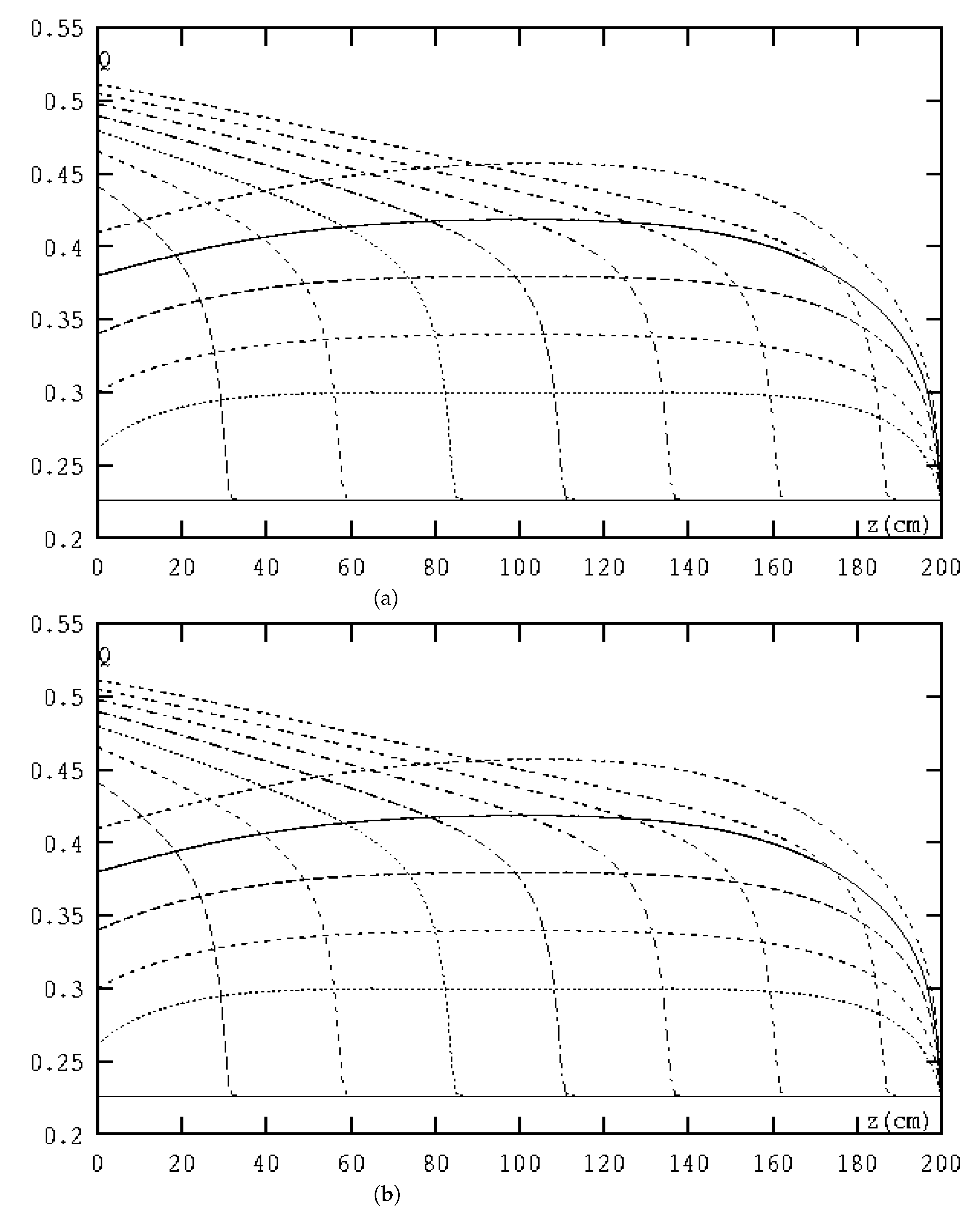
Figure 4.
(a) These curves are the MFE solutions of infiltration and evaporation water flux at h, 120 h,…, 420 h, 480 h,…, 840 h, respectively. (b) These curves are the MFE solutions of infiltration and evaporation water flux at h, 120 h,…, 420 h, 480 h,…, 840 h, respectively.
Figure 4.
(a) These curves are the MFE solutions of infiltration and evaporation water flux at h, 120 h,…, 420 h, 480 h,…, 840 h, respectively. (b) These curves are the MFE solutions of infiltration and evaporation water flux at h, 120 h,…, 420 h, 480 h,…, 840 h, respectively.

Table 1.
Twelve soil parameters in unsaturated water flow soil.
| Soil Types | /(mm) | /(mms) | b | ||
|---|---|---|---|---|---|
| 1 | 0.33 | 30 | 0.2000 | 3.5 | 0.088 |
| 2 | 0.36 | 30 | 0.0800 | 4.0 | 0.119 |
| 3 | 0.39 | 30 | 0.0032 | 4.5 | 0.151 |
| 4 | 0.42 | 200 | 0.0130 | 5.0 | 0.266 |
| 5 | 0.45 | 200 | 8.9 | 5.5 | 0.300 |
| 6 | 0.48 | 200 | 6.3 | 6.0 | 0.332 |
| 7 | 0.51 | 200 | 4.5 | 6.8 | 0.378 |
| 8 | 0.54 | 200 | 3.2 | 7.6 | 0.419 |
| 9 | 0.57 | 200 | 2.2 | 8.4 | 0.455 |
| 10 | 0.60 | 200 | 1.6 | 9.2 | 0.487 |
| 11 | 0.63 | 200 | 1.1 | 10.0 | 0.516 |
| 12 | 0.66 | 200 | 0.8 | 10.8 | 0.542 |
Table 2.
The comparison of CPU runtime and errors for the MFE solutions and the PPMFERD solutions.
| t | n | MFE Method | PPMFERD Method | ||
|---|---|---|---|---|---|
| CPU Runtime | CPU Runtime | ||||
| 210 h | 21 | 4462s | 62 s | ||
| 420 h | 42 | 8926s | 121 s | ||
| 630 h | 63 | 13393s | 182 s | ||
| 840 h | 84 | 17860s | 240 s | ||
Publisher’s Note: MDPI stays neutral with regard to jurisdictional claims in published maps and institutional affiliations. |
© 2022 by the authors. Licensee MDPI, Basel, Switzerland. This article is an open access article distributed under the terms and conditions of the Creative Commons Attribution (CC BY) license (https://creativecommons.org/licenses/by/4.0/).
Share and Cite
MDPI and ACS Style
Luo, Z.; Li, Y. A Preserving Precision Mixed Finite Element Dimensionality Reduction Method for Unsaturated Flow Problem. Mathematics 2022, 10, 4391. https://doi.org/10.3390/math10224391
AMA Style
Luo Z, Li Y. A Preserving Precision Mixed Finite Element Dimensionality Reduction Method for Unsaturated Flow Problem. Mathematics. 2022; 10(22):4391. https://doi.org/10.3390/math10224391
Chicago/Turabian StyleLuo, Zhendong, and Yuejie Li. 2022. "A Preserving Precision Mixed Finite Element Dimensionality Reduction Method for Unsaturated Flow Problem" Mathematics 10, no. 22: 4391. https://doi.org/10.3390/math10224391
Note that from the first issue of 2016, this journal uses article numbers instead of page numbers. See further details here.