
Adaptive Tracking Control Schemes for Fuzzy Approximation-Based Noncanonical Nonlinear Systems with Hysteresis Inputs

1
School of Automation, Guangdong University of Technology, Guangzhou 510006, China
2
School of Mechanical and Electrical Engineering, Guangzhou City Polytechnic, Guangzhou 510405, China
3
School of Computer Science & Engineering, South China University of Technology, Guangzhou 510006, China
*
Author to whom correspondence should be addressed.
Mathematics 2023, 11(14), 3253; https://doi.org/10.3390/math11143253
Submission received: 28 June 2023
/
Revised: 18 July 2023
/
Accepted: 19 July 2023
/
Published: 24 July 2023
(This article belongs to the Section Dynamical Systems)
Abstract
:In this paper, the tracking control problem of a class of fuzzy approximation-based noncanonical nonlinear systems with hysteresis inputs is investigated, where the fuzzy weight matrix is not available for measurement, and the hysteresis nonlinearities are modeled by the Prandtl–Ishlinskii operator. Due to the coupling effects, the plant input containing hysteresis is unknown. To solve the problem, two adaptive control schemes are developed. The first is a Lyapunov-based scheme, and the second is a gradient-based scheme. For convenience, only the relative-degree-one case is taken into account in design and analysis. With the proposed schemes, it can be proved that all signals in the closed-loop system are bounded, and the tracking error converges to a small region around zero. Simulation results show that the maximum steady-state error converges to and with two control schemes, which confirms the obtained results.
MSC:
37M051. Introduction
A class of smart materials such as piezoactuators with the advantages of high precision, high energy conversion efficiency, and fast response has received a lot of attention in the control field and has been used in many fields. In the application of high-precision positioning, the control problem of smart piezoelectric materials has been a research area of great interest. When using the piezoactuator for high-precision positioning, the nonlinear hysteresis effect exhibited by piezoelectric smart materials severely limits the performance of the piezoactuator, resulting in a loss of accuracy (as shown in [1,2,3,4,5,6]). A lot of research work has been carried out to address the control problem of output tracking for a class of systems with hysteresis inputs. It is common to model the system of a piezoactuator as a system model cascaded by a hysteresis dynamics system and an internal dynamics (including creep dynamics and vibration dynamics) system, and to construct the inverse of the model by identifying the system plant [7,8,9]. Further, more adaptive control schemes [10,11,12,13,14,15,16,17,18,19,20,21] are proposed to compensate for the hysteresis nonlinearity.
It is worth pointing out that the above solutions are proposed for a class of canonical-form systems with a hysteresis operator. For the control problem of canonical-form nonlinear systems with explicit relative degrees, the solutions are usually constructed on a Lyapunov-based backstepping design framework, whose main idea is to select appropriate Lyapunov functions and virtual control signals for each order of subsystems to ensure the stability of each subsystem, and then finally to derive and obtain the actual control signal. Therefore, the Lyapunov-based backstepping control schemes have been widely used in the control of canonical nonlinear systems [22,23,24,25,26,27]. However, the Lyapunov-based backstepping control scheme must first obtain the relative degree condition of the system, so it is only applicable to nonlinear systems in canonical form (i.e., with a strict feedback structure) or to a class of nonlinear systems that can be transformed into canonical form by a diffeomorphism. When the system is modeled as a cascade model of a noncanonical-form nonlinear system with a hysteresis operator, the design of a complete and effective adaptive control scheme is still an unsolved problem that needs to be paid attention to and solved.
We found inspiring ideas in the following works. In [28], the relative degree normal forms based on fuzzy approximation are established for a class of noncanonical nonlinear systems, and a new control framework based on feedback linearization theory is proposed. In [29], the Lyapunov-based and gradient-based feedback linearization techniques are extended to a class of noncanonical neural network systems and demonstrated excellent control results for such complex systems, which is enlightening. However, when the hysteresis model coupled with nonlinear systems is described as a linear term and a bounded disturbance-like term, the above solutions will not be applicable. On the one hand, the Lyapunov-based feedback linearization technique mentioned in [29] does not deal with the disturbance-like term presented in the output dynamic equation, resulting in difficulties in stability analysis, and on the other hand, when a gradient adaptive control scheme in the framework of the feedback linearization is used for updating adaptive parameters in the nonlinear system, the lack of adaptive modification for the disturbance-like term within the system will lead to a controller singularity problem and an accuracy loss problem. When the system is modeled as a cascade of hysteresis operators with a noncanonical nonlinear system, the design of a complete and efficient control scheme is an unsolved problem.
Motivated by the above research and unsolved technical drawbacks, in this paper, two different types of robust adaptive control schemes in the framework of feedback linearization are proposed to deal with the output tracking control problem of fuzzy approximation-based noncanonical nonlinear systems with unknown hysteresis inputs. One is a new Lyapunov-based adaptive control scheme, which adds a disturbance compensation term compared to the conventional scheme and can establish the whole performance analysis of the system. The other is a new gradient-based adaptive control scheme, which integrates the switching -modification to avoid the controller singularity problem and establish and robustify the disturbance-like term generated by the hysteresis modeling. Then, the proof procedure of the closed-loop signal boundedness for two schemes is given, and the performance analysis is established to demonstrate that the asymptotic tracking error converges to zero as time goes to infinity. A simulation example is given and the validity of our scheme is verified through simulation results. In summary, the proposed robust adaptive control schemes have the following technical contributions:
- (1)
- For a class of noncanonical nonlinear systems cascaded by a hysteresis operator with uncertain parameters, we use a fuzzy logic system to deal with the technical issues caused by the unknown nonlinear part for reducing the influence of the unknown nonlinear factors on the control system and develop a new control scheme based on Lyapunov and feedback linearization techniques, such that the hysteresis disturbance terms possessed within the system are compensated to obtain the desired output tracking performance.
- (2)
- A more general gradient-based adaptive parameter updating with integrated switching -modification compensation is developed, which can avoid the controller singularity and robustify the bounded disturbances generated by the hysteresis decomposition. Our scheme based on fuzzy approximation can solve the output tracking problem of noncanonical nonlinear systems with unknown hysteresis inputs. We verify the output tracking performance of our scheme through the simulation results and demonstrate the robustness of our scheme to disturbance.
- (3)
- We have performed the strict signal boundedness proof and system stability analysis for both proposed control schemes, which ensures the reliability of the proposed control schemes.
The rest of the paper is structured as follows. The control problem to be investigated and basic knowledge will be given in the following section. In Section 3, we give the relative degree normal forms for the noncanonical systems and the derivation procedure for the stability of zero dynamic subsystem. In Section 4, we present two different adaptive control schemes, Lyapunov-based and gradient-based, to address the output tracking problem of the system with relative degree one. After that, the validity of our scheme is illustrated by the simulation results presented in Section 5. The full paper is summarized in Section 6. Then, we need to define some mathematical notations used in this paper. For a vector signal :
- ;
- has the following form:
- , denoting signal norm, has the following form:
2. Problem Formulation and Preliminaries
In this section, we investigate the control problem of the noncanonical form system cascaded by the hysteresis operator and briefly review some basic knowledge about the hysteresis operator and fuzzy approximation.
2.1. Plant Formulation
A class of noncanonical-form nonlinear systems cascaded by a hysteresis operator is considered as follows:
where is an unparameterizable unknown smooth function; denote the system state vector and system output, respectively; and denote the unknown control matrix and output matrix; and applied directly to the system plant contains the actual control input , which has been cascaded by a hysteresis operator. The block diagram of the noncanonical nonlinear system cascaded by the hysteresis model considered in this paper is shown in Figure 1.
Next, referring to [30], we present the basic operator and model describing the hysteresis nonlinearity. The classical hysteresis Prandtl–Ishlinskii (PI) model is a general model for describing hysteresis effects and consists of play operator and density function . Firstly, we formulate the basic play operator (whose structure is shown in Figure 2) as follows.
The play operator: Suppose the hysteresis inputs are monotone in each sub-time domain on . Then, the operator can be expressed as
where , and is the jth operator threshold, which is expressed as
where m denotes the number of operators.
The PI model: The PI model, characterized by the play operator, can be modeled as the following mathematical expression:
where is a constant. For facilitating further design and analysis, referring to the conclusions derived from [31], the PI model can be formulated as
where is the linear term, and another term denotes the nonlinear part, which satisfies with a bounded constant M. Figure 3 indicates the hysteresis curve presented by PI model (5) with the inputs , density function , and the number of the operators is 30.
2.2. Noncanonical Fuzzy Approximation-Based Model
Since the unparameterizable function in the plant (1) is unknown, it is not trivial to develop a control scheme for the system cascaded by a hysteresis operator. For addressing this problem and guaranteeing the integrity of the original system performance as much as possible, from the research of fuzzy approximation [32,33,34], a new controlled plant can be approximated by the fuzzy logic system, which can be expressed as
where , represents a desired weight matrix, and is a vector of fuzzy basis function constructed from
where is a Gaussian fuzzy function with the constants .
2.3. Control Objective
The goal of our control scheme is to design the adaptive laws to generate a control signal for system (6) with a hysteresis operator, ensuring the boundedness of all signals and for any bounded desired signal .
Remark 1.
When using the fuzzy system to approximate the system (1), there is an approximation error of the model, which can theoretically be eliminated by higher-precision approximation, but this will result in a larger computation. For the convenience of the subsequent analysis, the performance of the fuzzy approximation-based system (6) is considered to be identical to the original system (1), which means that the approximation error is neglected in the process of using fuzzy logic approximation. Therefore, the case that the error exists in the process of approximation should be further investigated.
3. Relative Degree Norms and the Stability of Zero Dynamics Subsystem
With the knowledge of feedback linearization, in this section, we define the relative degree norms for noncanonical fuzzy approximation-based systems (6) and derive the applicable conditions for different relative degree cases. Then, we perform the stability analysis for dynamic subsystems within the system.
3.1. System Relative Degree Norms
Defining and , with the approximation equation derived above, the fuzzy approximation-based noncanonical system (6) is rewritten as
which is a non-strict feedback system. Then, the relative degree norms based on the system (8) can be established, and the applicable conditions of various forms are derived.
Definition 1.
By iterating the time derivative of , we derive the relative degree norms for the fuzzy approximation-based system (8) with noncanonical-form until an explicit relationship is established between ρ-order time derivatives and the control input . Specifically, the nonlinear system (8) is regarded as having a relative degree ρ if the Lie-derivative satisfies
where with for denotes the kth-order Lie derivative, and the has the similar forms. Then, we derive the following applicable conditions for different relative degree cases based on the above definition.
Lemma 1.
3.2. Dynamics Subsystem
The feedback linearization technique can be applied to systems in which the state variables match the relative degrees. However, when the relative degree of the system (8) is less than the state variable n, the feedback linearization technique is difficult to apply to this system. In this case, the system (8) will involve a zero dynamics subsystem independent of the control signal, which is expressed as
where is a nonlinear function; ; and denotes the zero dynamic subsystem, which can be obtained from
where . For the subsequent control design and analysis to proceed successfully, the stability of the zero dynamics subsystem (12) without input signals requires the following assumption to be guaranteed.
Assumption 1.
The nonlinear function assumes that the partial derivative is bounded, and satisfies
where is normally chosen to be a positive constant, and is seen as a bounded disturbance-like term.
According to Assumption 1, we can derive that for some positive constants . It is not difficult to conclude that the boundedness of can be guaranteed if is bounded. The assumption and similar argument are described in detail in [35].
Remark 2.
In the following parts, we focus on the relative degree one case, and develop two different adaptive control schemes to settle the control problem of the fuzzy approximation-based system (6) with the unknown hysteresis inputs. The case with higher relative degrees will involve more preliminaries, and the stability analysis is very complicated. Therefore, the control problem for the fuzzy approximation-based system cascaded by a hysteresis operator with higher relative degrees needs to be further investigated.
4. Control Design for Fuzzy Approximation-Based System with Relative Degree One
Based on the above analysis, we mainly investigate the relative degree case and develop a Lyapunov-based adaptive control method with disturbance compensation and a gradient-based method integrated switch -modification adaptive control scheme in the framework of the feedback linearization to meet the desired output tracking performance demands. The system block diagram of our scheme is shown in Figure 4.
4.1. Plant Description and Nominal Control Scheme
From Lemma 1 and the PI model (5) when , the tracking dynamics of the system (6) is represented as
where is an unknown modeling error, which can be considered as a bounded disturbance-like term. When the system parameters , and are known, we choose the nominal controller
where , denotes the tracking error, and a is a positive design parameter. However, the nominal controller (16) based on the feedback linearization technique is not applicable when the system parameters are unknown, so it is essential to design a new control scheme for updating the unknown parameters to achieve the desired values. In this case, we need to parameterize the model (15), from which it follows that
where . It is notable that the parameterization technique is important for the design of subsequent adaptive laws, especially in adaptive control for the noncanonical uncertain system.
4.2. Lyapunov-Based Adaptive Control Scheme
We first describe the design of the Lyapunov-based adaptive law for updating and demonstrate that the tracking error is convergent.
4.2.1. Adaptive Update Law for
The Lyapunov-based adaptive controller is designed as follows:
where , and are the estimated values of , and in the nominal controller (17); is selected as an integrable signal. Substituting the adaptive controller (18) into the parameterized model (17), the following equation is established:
where denotes the estimated error.
Remark 3.
In the process of parameter updating, there is a lack of constraints on the parameter adaptation range, and the case of being zero at some points may occur, resulting in a controller singularity problem. To overcome this technical issue, a parameter projection method, described in [36], is proposed to modify the parameter adaptive estimation of . Due to limitations in the length of this paper, the details of this procedure will be omitted.
To address the issue of adaptive updating of parameters, we propose the following adaptive laws to update and :
where and are adaptive gains.
4.2.2. Performance Analysis
The asymptotic tracking performance of the dynamic system (15) with the disturbance-like term is established with the adaptive laws (20) and (21) and the tracking error Equation (19). For deriving the main results, we need to make the following assumption.
Assumption 2.
The sign of is known and generally positive.
With Assumption 2 holding, the problem of unknown control direction has been circumvented. Then, the following results can be established.
Theorem 1.
Proof.
The proper positive function is selected as
where . Then, the first-order time derivatives with (20) and (21) can be further computed as
Incorporating the fact that is integrable and is bounded, we obtain , which can further derive that , and belong to . When , from Assumption 1, it implies that . Since , the state vector , which can derive that the control signal by (18), and we have the hysteresis output by (5). So far, we have verified the signal stability of the system. Integrating both sides of (23) and combining the properties of and , we obtain that . We can also derive that is bounded by (22). Incorporated with Barbalat’s lemma, we obtain that as time . □
4.3. Gradient-Based Adaptive Control Scheme
For achieving our control objective, another more general gradient algorithm for the fuzzy approximation-based system (6) with is developed to address the issue of adaptive updating for unknown parameters.
4.3.1. Adaptive Update Law for
When the parameters are unknown in the system (6), we develop the following adaptive controller:
where , and a denote the controller design parameters, and is the adaptive parameter, which are identical to that in (18). Substituting (24) into the parameterized model (17), we have
Ignoring the effect of the exponentially decaying term associated with the initial response, we derive that
where , and , and it is not difficult to verify since is stable and is bounded by (15). For the design of the adaptive laws, we establish the estimation error system
with . Incorporated with the tracking error (26), we derive
Then, a gradient-based adaptive parameter update law with leakage term for updating is designed as
where is a constant adaptation gain; ; denotes a leakage term with switching -modification function , which is defined as
where and are design parameters, and should satisfy . For the adaptive laws (29), we have
which is crucial since it facilitates the subsequent performance analysis.
4.3.2. Properties of Estimated Parameters and Performance Analysis
The stability of the system with is established in this part, while the case of can be demonstrated by applying our control scheme to a simulation example to prove the robustness of this scheme. We first summarize the properties of the gradient-based adaptive laws (29) to establish the complete performance analysis.
Proposition 1.
The proposed adaptive parameter update law (29) ensures that the signals have the following properties: belongs to , , and .
Proof.
We choose the proper positive function as
whose first-order time derivatives with the adaptive law (29) are derived as
with the inequality (31) and . It is not difficult to conclude that and belong to from the result (33). Furthermore, based on (27) and defined in (29), we obtain that
which indicates . In view of (29) and (34), we have
which implies . Integrating both sides of (33), we derive that
from which it follows that with the inequality (34). Furthermore, it is not hard to verify based on (36). □
Before giving the main results, the following assumptions need to be made.
Assumption 3.
The fuzzy basis function vector , the time derivative , the partial derivatives , and are bounded.
Assumption 4.
The sign of and are known and considered to be positive generally.
Assumption 3 can derive that with and are bounded, which is essential for the subsequent stability analysis. And Assumption 4 means that we can avoid the unknown direction problem in designing the controller.
With the above properties and under Assumptions 3 and 4, the following results can be concluded.
Theorem 2.
Suppose that Assumptions 3 and 4 hold, the gradient-based robust adaptive control scheme ensures the signal boundedness of the system (6) with and , and the tracking error satisfies that as .
Proof.
We first give the following notations before proceeding with the proof: , a proper bounded constant; , a generic function; , a generic function satisfying . The expression of the stable transfer function is
Note that and , from which it can be derived that and are also stable transfer functions. Using the Swapping Lemma in [35] for the last two terms in (27), we have
Using the property that in Proposition 1 and the fact that is a stable transfer function, we have
Then, using Lemma A1 in Appendix A and the fact that is a stable transfer function, the following inequality is established
Recalling , we denote the state vector . Then, the tracking error Equation (26) with is expressed as
Since in Proposition 1, and the transfer function is strictly proper, we obtain that
From Assumption 1, it implies that
Note that is a diffeomorphism with and , and we have
and it is not derived that
Incorporated with the boundedness of , we can derive
Since the components of are shown as (17), and under Assumption 3, the and satisfy that
Incorporated with (46), the regular signal satisfies that
Since with a strictly proper transfer function, using Lemma A2, we have
Defining , similar to the proof of the property of , we can verify that
where satisfies that . Then, we can derive that
Incorporated with being bounded and (49), there exists a satisfying . Then, it is not difficult to derive that
From Lemma A1 and the properties of , it follows that , and further
Since , the following inequalities are established:
and
Since the satisfying , along with (58), we can verify that , which implies . Then, it is not difficult to derive that is bounded by the inequality (56). Incorporated with (42)–(44), we obtain that , and are bounded, which can derive . In summary, all signals in the system (15) have been verified to belong to , and the tracking performance has been established. □
5. Simulation Results
For demonstrating the performance of our scheme, we applied this scheme to a simulation example. First, we consider the system as a second-order system with , which follows . Then, the origin system parameters are set in the system (1) as
The fuzzy approximation-based noncanonical nonlinear system (6) can be substituted for the system (1) when the system performance is considered to meet the requirements. Then, by referring to the fuzzy approximation algorithm in [37], we can define the weight matrix and the fuzzy basis function as
and the matrix A is chosen as the following form to satisfy Hurwitz stability:
It is noted that the system parameters , and are considered to be unknown, and the values within and may not be optimal choices, but they can meet the simulation performance requirements.
5.1. Simulation Results of Lyapunov-Based Control Scheme
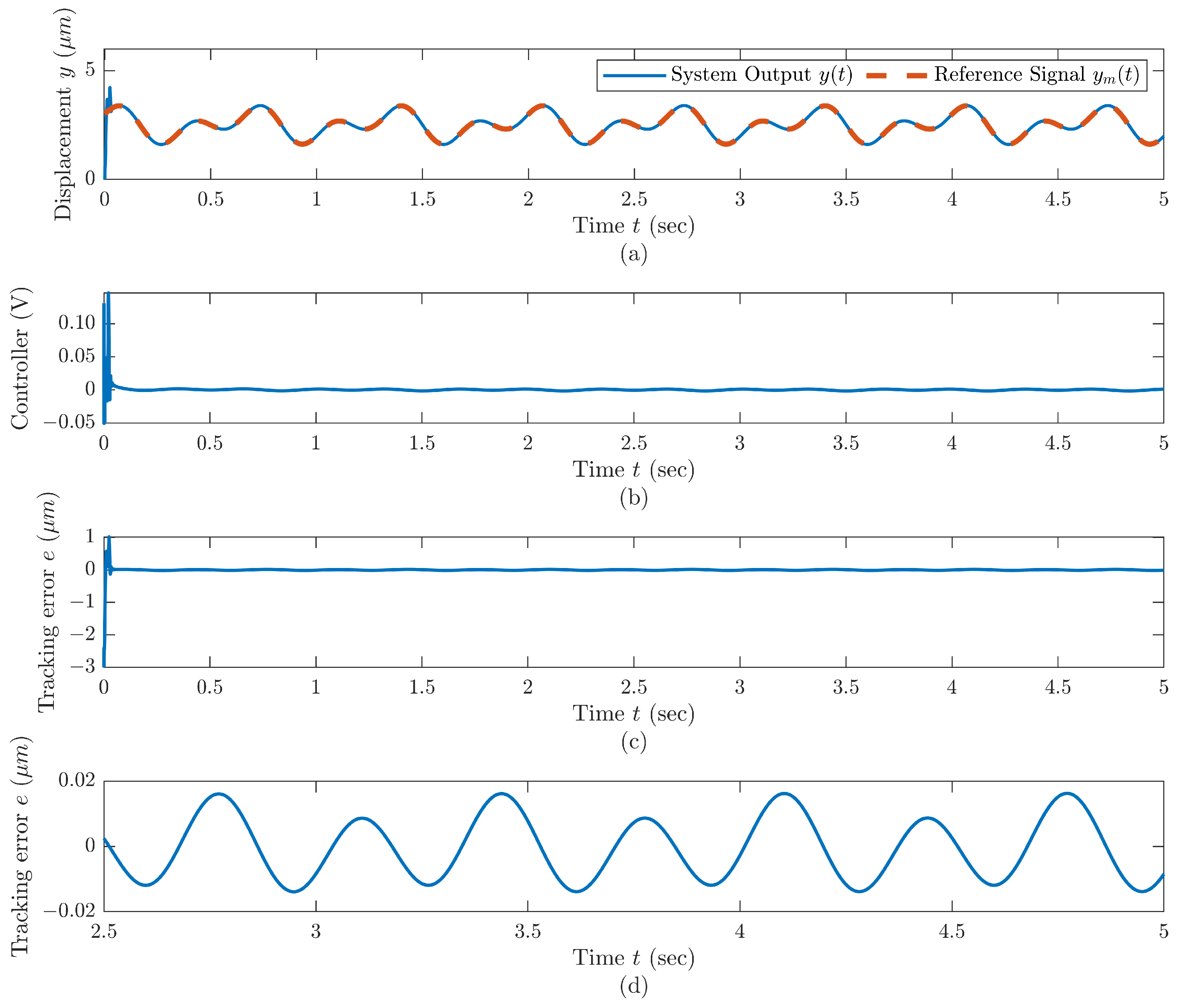
Considering the controller (18), we set the and controller design parameters . We set the initial values of the adaptive parameters as , and a desired signal is selected as . For the choices of adaptive gains and , we set , and the results of tracking error corresponding to each adaptive gain are shown in Figure 5. Figure 5 shows that the interval of tracking error can converge as the adaptive gains increase, but when the gains increase to some certain value (e.g., ), the problem of controller singularity occurs, resulting in a poor control effect. Therefore, after several parameter adjustments, we choose the appropriate adaptive gains , and Figure 6 presents the system tracking performance and the steady-state error converges to .
5.2. Simulation Results of Gradient-Based Control Scheme
For more reasonably verifying the validity of the gradient-based control scheme, we use the same reference signal, system states, and fuzzy basic function as in Section 5.1. In the setting of the parameters, we find that if N in (30) is small, the controller singularity problem (as seen in Figure 5) will occur. In order to avoid the possible singularity problem in the adaptive parameter updating of the controller, we find a suitable set of switch -modification design parameters after several adjustments. Then, we set the controller design parameter and the adaptive gain after several parameter adjustments. The initial values of are set as . Figure 7 shows the system tracking performance with the gradient-based adaptive law for updating the adaptive parameters, and the tracking error can converge to a very small interval , which implies that Proposition 1 is confirmed.
From the above results, it can be seen that for two different types of adaptive control schemes, the output of the system (6) with hysteresis inputs can track the bounded desired signals asymptotically, which indicates the efficiency and robustness of our scheme.
Remark 4.
The reason for setting the controller design parameters in Section 5.1 is that in the simulation, we find that the dominant effect on the controller output is in Equation (18), and we try to increase a and ϱ, but the tracking effect changes little, and finally, we set them as 1. In Section 5.2, the reason for setting is similar.
6. Conclusions
We investigate the control problem of a class of hysteresis dynamics system coupled with an unknown noncanonical nonlinear system and the compensation problem of the disturbance term presented by the hysteresis formulation, and propose a Lyapunov-based method with error modification adaptive control scheme and a gradient-based method with integrated switch -modification control scheme in the framework of the feedback linearization. In our solution, all signals in the fuzzy approximation-based system with a hysteresis operator are guaranteed to be bounded, and the system can achieve the desired performance, which indicates the robustness of our scheme to disturbance. Through simulation, the above results improve the tracking accuracy by compared to the minimum steady-state error achieved by another adaptive control scheme [38].
Author Contributions
Conceptualization, G.L.; methodology, W.Y.; software, K.Z.; validation, G.L. and K.Z.; formal analysis, K.Z.; writing—original draft preparation, W.Y.; writing—review and editing, W.Y., K.Z. and X.S. All authors have read and agreed to the published version of the manuscript.
Funding
This research was funded by the Tertiary Education Scientific research project of Guangzhou Municipal Education Bureau [No. 202235364], and the Special projects in key fields of colleges and universities in Guangdong Province [No. 2021ZDZX1109], and the Research project of Guangzhou City Polytechnic [No. KYTD2023004], and the National Natural Science Foundation of China [No. 6210021076], and the Guangzhou Municipal Science and Technology Project [No. 202201010381].
Institutional Review Board Statement
Not applicable.
Informed Consent Statement
Not applicable.
Data Availability Statement
Not applicable.
Acknowledgments
Not applicable.
Conflicts of Interest
The authors declare no conflict of interest.
Appendix A
Some lemmas required in the proof of the above stability analysis are given in the Appendix, and the details of their proof are given in [35]. The notations , and defined in the text are used in this part.
Lemma A1.
Let with a stable transfer function . If
then
Furthermore, if is strictly a proper transfer function, we have
Lemma A2.
Let with a stable transfer function . If , and satisfies
then we have
References
- Jin, H.; Gao, X.; Ren, K.; Liu, J.; Qiao, L.; Liu, M.; Chen, W.; He, Y.; Dong, S.; Xu, Z.; et al. Review on Piezoelectric Actuators Based on High-Performance Piezoelectric Materials. IEEE Trans. Ultrason. Ferroelectr. Freq. Control 2022, 69, 3057–3069. [Google Scholar] [CrossRef] [PubMed]
- Chen, J.; Peng, G.; Hu, H.; Ning, J. Dynamic Hysteresis Model and Control Methodology for Force Output Using Piezoelectric Actuator Driving. IEEE Access 2020, 8, 205136–205147. [Google Scholar] [CrossRef]
- Feng, Y.; Li, Y. System Identification of Micro Piezoelectric Actuators via Rate-Dependent Prandtl-Ishlinskii Hysteresis Model Based on a Modified PSO Algorithm. IEEE Trans. Nanotechnol. 2021, 20, 205–214. [Google Scholar] [CrossRef]
- Xu, R.; Zhang, X.; Guo, H.; Zhou, M. Sliding Mode Tracking Control with Perturbation Estimation for Hysteresis Nonlinearity of Piezo-Actuated Stages. IEEE Access 2018, 6, 30617–30629. [Google Scholar] [CrossRef]
- Dong, R.; Tan, Y.; Xie, Y.; Janschek, K. Recursive Identification of Micropositioning Stage Based on Sandwich Model with Hysteresis. IEEE Trans. Control Syst. Technol. 2017, 25, 317–325. [Google Scholar] [CrossRef]
- Croft, D.; Shed, G.; Devasia, S. Creep, hysteresis, and vibration compensation for piezoactuators: Atomic force microscopy application. J. Dyn. Sys. Meas. Control 2001, 123, 35–43. [Google Scholar] [CrossRef]
- Wen, Z.; Ding, Y.; Liu, P.; Ding, H. An Efficient Identification Method for Dynamic Systems with Coupled Hysteresis and Linear Dynamics: Application to Piezoelectric-Actuated Nanopositioning Stages. IEEE/ASME Trans. Mechatron. 2019, 24, 326–337. [Google Scholar] [CrossRef]
- Li, Z.; Shan, J. Inverse Compensation Based Synchronization Control of the Piezo-Actuated Fabry–Perot Spectrometer. IEEE Trans. Ind. Electron. 2017, 64, 8588–8597. [Google Scholar] [CrossRef]
- Leang, K.K.; Devasia, S. Feedback-Linearized Inverse Feedforward for Creep, Hysteresis, and Vibration Compensation in AFM Piezoactuators. IEEE Trans. Control Syst. Technol. 2007, 15, 927–935. [Google Scholar] [CrossRef]
- Zhu, Z.; Pan, Y.; Zhou, Q.; Lu, C. Event-Triggered Adaptive Fuzzy Control for Stochastic Nonlinear Systems with Unmeasured States and Unknown Backlash-Like Hysteresis. IEEE Trans. Fuzzy Syst. 2021, 29, 1273–1283. [Google Scholar] [CrossRef]
- Wang, H.; Shen, L. Adaptive Fuzzy Fixed-Time Tracking Control for Nonlinear Systems with Time-Varying Full-State Constraints and Actuator Hysteresis. IEEE Trans. Fuzzy Syst. 2023, 31, 1352–1361. [Google Scholar] [CrossRef]
- Wu, Y.; Ma, H.; Chen, M.; Li, H. Observer-Based Fixed-Time Adaptive Fuzzy Bipartite Containment Control for Multiagent Systems with Unknown Hysteresis. IEEE Trans. Fuzzy Syst. 2022, 30, 1302–1312. [Google Scholar] [CrossRef]
- Zhang, X.; Xu, H.; Chen, X.; Li, Z.; Su, C.Y. Modeling and Adaptive Output Feedback Control of Butterfly-like Hysteretic Nonlinear Systems with Creep and Their Applications. IEEE Trans. Ind. Electron. 2023, 70, 5182–5191. [Google Scholar] [CrossRef]
- Liu, L.; Tang, L. Partial State Constraints-Based Control for Nonlinear Systems with Backlash-Like Hysteresis. IEEE Trans. Syst. Man Cybern. Syst. 2020, 50, 3100–3104. [Google Scholar] [CrossRef]
- Namadchian, Z.; Rouhani, M. Adaptive Neural Tracking Control of Switched Stochastic Pure-Feedback Nonlinear Systems with Unknown Bouc–Wen Hysteresis Input. IEEE Trans. Neural Netw. Learn. Syst. 2018, 29, 5859–5869. [Google Scholar] [CrossRef]
- Liu, Y.J.; Tong, S.; Chen, C.L.P.; Li, D.J. Neural Controller Design-Based Adaptive Control for Nonlinear MIMO Systems with Unknown Hysteresis Inputs. IEEE Trans. Cybern. 2016, 46, 9–19. [Google Scholar] [CrossRef]
- Al-Nadawi, Y.K.; Tan, X.; Khalil, H.K. Inversion-Free Hysteresis Compensation via Adaptive Conditional Servomechanism with Application to Nanopositioning Control. IEEE Trans. Control Syst. Technol. 2021, 29, 1922–1935. [Google Scholar] [CrossRef]
- Lu, K.; Liu, Z.; Chen, C.L.P.; Zhang, Y. Adaptive Inverse Compensation for Unknown Input and Output Hysteresis Using Output Feedback Neural Control. IEEE Trans. Syst. Man Cybern. Syst. 2022, 52, 3224–3236. [Google Scholar] [CrossRef]
- Wang, J.; Liu, Z.; Zhang, Y.; Chen, C.L.P. Neural Adaptive Event-Triggered Control for Nonlinear Uncertain Stochastic Systems with Unknown Hysteresis. IEEE Trans. Neural Netw. Learn. Syst. 2019, 30, 3300–3312. [Google Scholar] [CrossRef]
- Yu, T.; Ma, L.; Qin, N. Adaptive Cooperative Tracking Control of Multi-Agent Systems with Unknown Actuators Hysteresis. IEEE Access 2018, 6, 33015–33028. [Google Scholar] [CrossRef]
- Zhang, X.; Jing, R.; Li, Z.; Li, Z.; Chen, X.; Su, C.Y. Adaptive Pseudo Inverse Control for a Class of Nonlinear Asymmetric and Saturated Nonlinear Hysteretic Systems. IEEE/CAA J. Autom. Sin. 2021, 8, 916–928. [Google Scholar] [CrossRef]
- Lai, G.; Zhang, Y.; Liu, Z.; Chen, C.L.P. Indirect Adaptive Fuzzy Control Design with Guaranteed Tracking Error Performance For Uncertain Canonical Nonlinear Systems. IEEE Trans. Fuzzy Syst. 2019, 27, 1139–1150. [Google Scholar] [CrossRef]
- Lai, G.; Zhang, Y.; Liu, Z.; Wang, J.; Chen, K.; Chen, C.L.P. Direct Adaptive Fuzzy Control Scheme with Guaranteed Tracking Performances for Uncertain Canonical Nonlinear Systems. IEEE Trans. Fuzzy Syst. 2022, 30, 818–829. [Google Scholar] [CrossRef]
- Wu, J.; Lu, Y. Adaptive Backstepping Sliding Mode Control for Boost Converter with Constant Power Load. IEEE Access 2019, 7, 50797–50807. [Google Scholar] [CrossRef]
- Yueneng, Y.; Ye, Y. Backstepping sliding mode control for uncertain strict-feedback nonlinear systems using neural-network-based adaptive gain scheduling. J. Syst. Eng. Electron. 2018, 29, 580–586. [Google Scholar]
- Xu, Z.; Zhao, L. Error-Based Gain-Varying Finite-Time Command Filtered Backstepping Control for Nonlinear Systems with Disturbances. IEEE Trans. Circuits Syst. II Express Briefs 2022, 69, 2917–2921. [Google Scholar] [CrossRef]
- Yu, X.; Lin, Y. Adaptive Backstepping Quantized Control for a Class of Nonlinear Systems. IEEE Trans. Autom. Control 2017, 62, 981–985. [Google Scholar] [CrossRef]
- Zhang, Y.; Tao, G.; Chen, M. Relative Degrees and Adaptive Feedback Linearization Control of T–S Fuzzy Systems. IEEE Trans. Fuzzy Syst. 2015, 23, 2215–2230. [Google Scholar] [CrossRef]
- Zhang, Y.; Tao, G.; Chen, M. Adaptive Neural Network Based Control of Noncanonical Nonlinear Systems. IEEE Trans. Neural Netw. Learn. Syst. 2016, 27, 1864–1877. [Google Scholar] [CrossRef] [PubMed]
- Rakotondrabe, M. Classical Prandtl-Ishlinskii modeling and inverse multiplicative structure to compensate hysteresis in piezoactuators. In Proceedings of the 2012 American Control Conference (ACC), Montreal, QC, Canada, 27–29 June 2012; pp. 1646–1651. [Google Scholar]
- Su, C.Y.; Wang, Q.; Chen, X.; Rakheja, S. Backstepping based variable structure control of a class of nonlinear systems preceded by hysteresis. In Proceedings of the 2005 International Conference on Control and Automation, Budapest, Hungary, 26–29 June 2005; Volume 1, pp. 288–292. [Google Scholar]
- Wang, H.; Liu, X.; Liu, K.; Karimi, H.R. Approximation-Based Adaptive Fuzzy Tracking Control for a Class of Nonstrict-Feedback Stochastic Nonlinear Time-Delay Systems. IEEE Trans. Fuzzy Syst. 2015, 23, 1746–1760. [Google Scholar] [CrossRef]
- Liu, Y.J.; Tong, S. Adaptive Fuzzy Identification and Control for a Class of Nonlinear Pure-Feedback MIMO Systems with Unknown Dead Zones. IEEE Trans. Fuzzy Syst. 2015, 23, 1387–1398. [Google Scholar] [CrossRef]
- Zhao, X.; Wang, X.; Zong, G.; Li, H. Fuzzy-Approximation-Based Adaptive Output-Feedback Control for Uncertain Nonsmooth Nonlinear Systems. IEEE Trans. Fuzzy Syst. 2018, 26, 3847–3859. [Google Scholar] [CrossRef]
- Sastry, S.; Bodson, M.; Bartram, J.F. Adaptive Control: Stability, Convergence, and Robustness; Prentice Hall: Englewood Cliffs, NJ, USA, 1990. [Google Scholar]
- Tao, G. Adaptive Control Design and Analysis; John Wiley & Sons: Hoboken, NJ, USA, 2003; Volume 37. [Google Scholar]
- Chen, B.; Liu, X.P.; Ge, S.S.; Lin, C. Adaptive Fuzzy Control of a Class of Nonlinear Systems by Fuzzy Approximation Approach. IEEE Trans. Fuzzy Syst. 2012, 20, 1012–1021. [Google Scholar] [CrossRef]
- Chen, X.; Su, C.Y.; Li, Z.; Yang, F. Design of Implementable Adaptive Control for Micro/Nano Positioning System Driven by Piezoelectric Actuator. IEEE Trans. Ind. Electron. 2016, 63, 6471–6481. [Google Scholar] [CrossRef]
Figure 1.
The block diagram of the piezoactuator system.
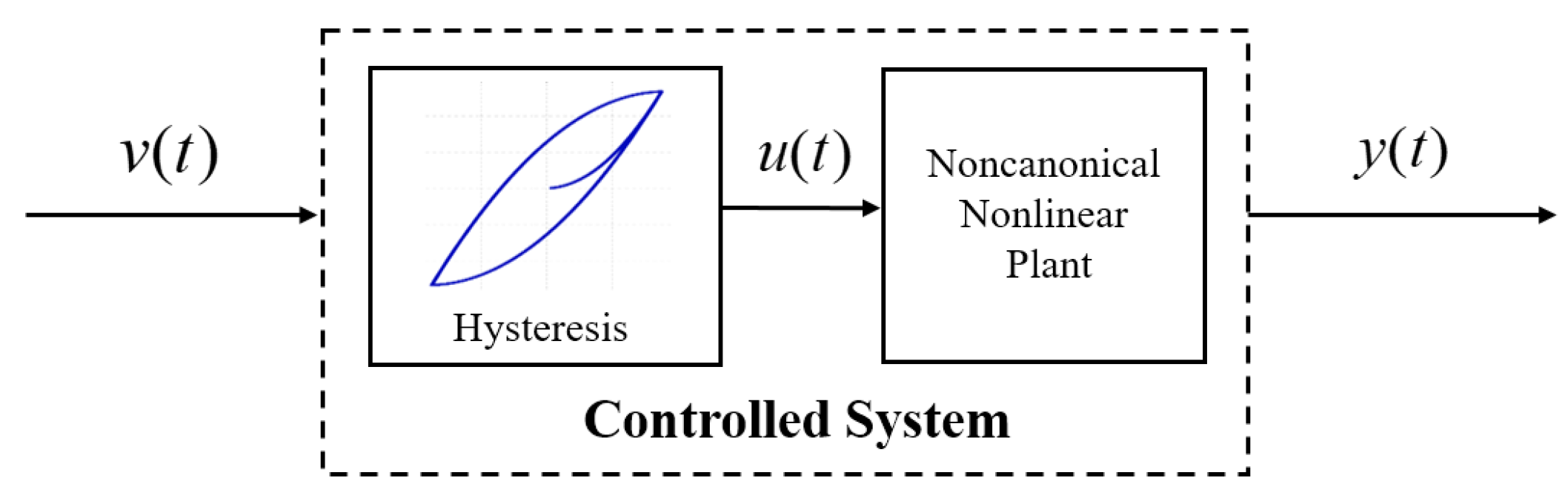
Figure 2.
Play operator structure.
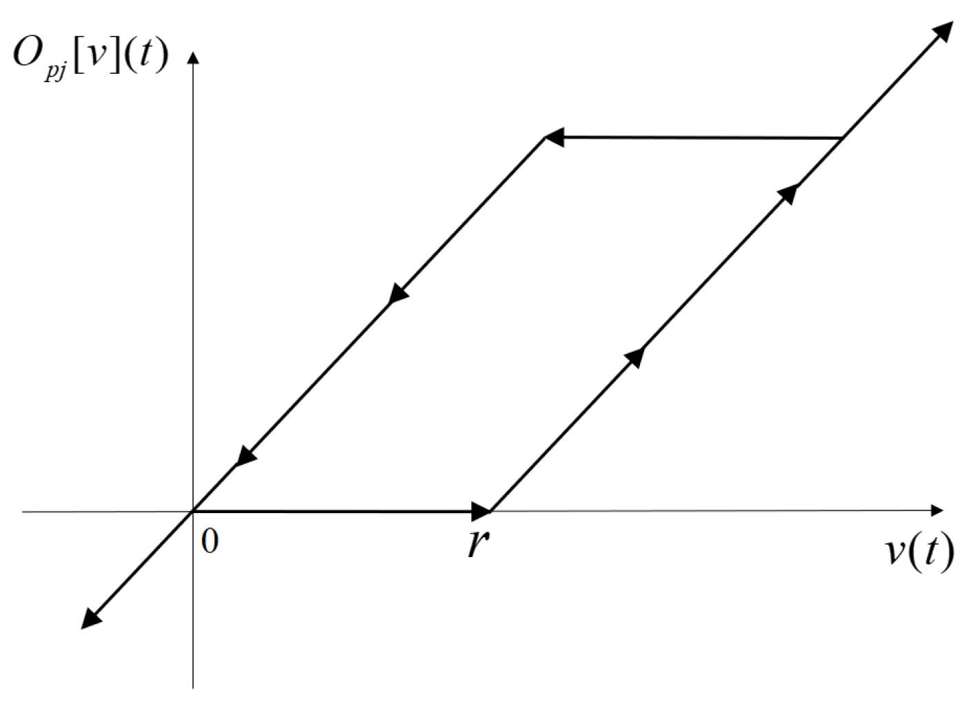
Figure 3.
Hysteresis curve.

Figure 4.
The system block diagram of our control scheme.

Figure 5.
Tracking error (in the second half of the time) corresponds to different adaptive gains.
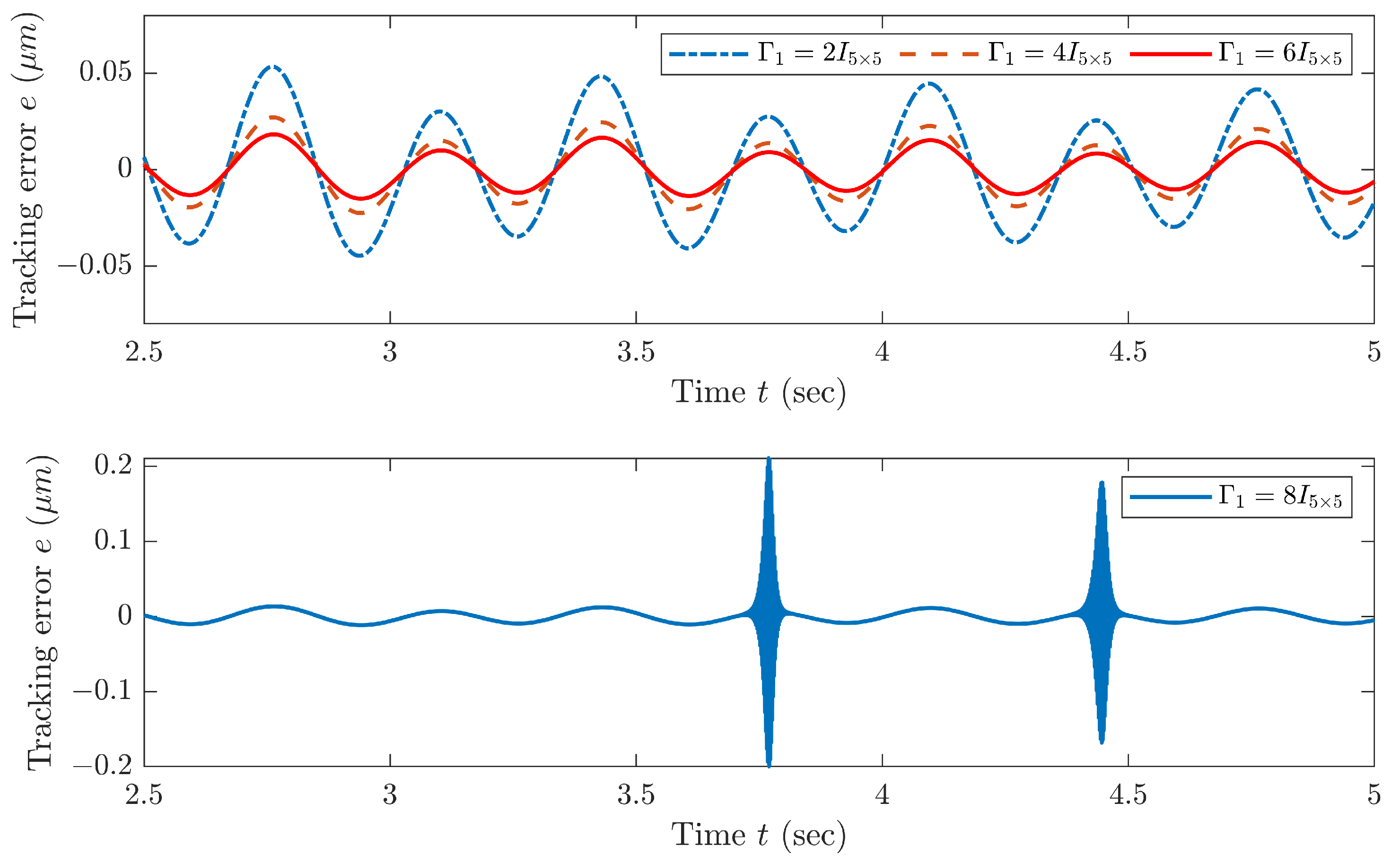
Figure 6.
(a) Tracking performance of the system (1) with the Lyapunov-based control scheme. (b) Controller output. (c) Tracking error. (d) Tracking error in the second half of the time.
Figure 6.
(a) Tracking performance of the system (1) with the Lyapunov-based control scheme. (b) Controller output. (c) Tracking error. (d) Tracking error in the second half of the time.
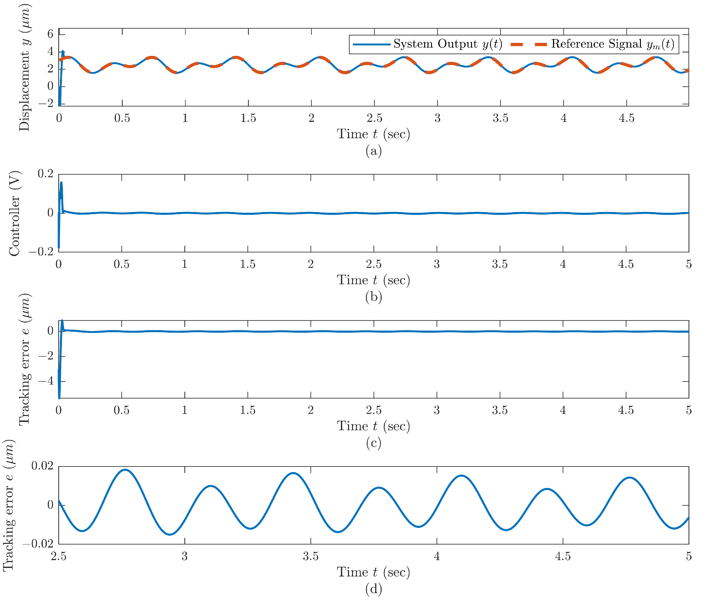
Figure 7.
(a) Tracking performance of the system (1) with the gradient-based control scheme. (b) Controller output. (c) Tracking error. (d) Tracking error in the second half of the time.
Figure 7.
(a) Tracking performance of the system (1) with the gradient-based control scheme. (b) Controller output. (c) Tracking error. (d) Tracking error in the second half of the time.
Disclaimer/Publisher’s Note: The statements, opinions and data contained in all publications are solely those of the individual author(s) and contributor(s) and not of MDPI and/or the editor(s). MDPI and/or the editor(s) disclaim responsibility for any injury to people or property resulting from any ideas, methods, instructions or products referred to in the content. |
© 2023 by the authors. Licensee MDPI, Basel, Switzerland. This article is an open access article distributed under the terms and conditions of the Creative Commons Attribution (CC BY) license (https://creativecommons.org/licenses/by/4.0/).
Share and Cite
MDPI and ACS Style
Lai, G.; Zeng, K.; Yang, W.; Su, X. Adaptive Tracking Control Schemes for Fuzzy Approximation-Based Noncanonical Nonlinear Systems with Hysteresis Inputs. Mathematics 2023, 11, 3253. https://doi.org/10.3390/math11143253
AMA Style
Lai G, Zeng K, Yang W, Su X. Adaptive Tracking Control Schemes for Fuzzy Approximation-Based Noncanonical Nonlinear Systems with Hysteresis Inputs. Mathematics. 2023; 11(14):3253. https://doi.org/10.3390/math11143253
Chicago/Turabian StyleLai, Guanyu, Kairong Zeng, Weijun Yang, and Xiaohang Su. 2023. "Adaptive Tracking Control Schemes for Fuzzy Approximation-Based Noncanonical Nonlinear Systems with Hysteresis Inputs" Mathematics 11, no. 14: 3253. https://doi.org/10.3390/math11143253
Note that from the first issue of 2016, this journal uses article numbers instead of page numbers. See further details here.