
Transport Object Detection in Street View Imagery Using Decomposed Convolutional Neural Networks


1
Department of Computer Science, Aberystwyth University, Aberystwyth SY23 3DB, UK
2
School of Computer Science, Northwestern Polytechnical University, Xi’an 710129, China
3
School of Information Engineering, Fujian Business University, Fuzhou 350506, China
4
Information Office, Chongqing University of Science and Technology, Chongqing 401331, China
*
Authors to whom correspondence should be addressed.
Mathematics 2023, 11(18), 3839; https://doi.org/10.3390/math11183839
Submission received: 3 August 2023
/
Revised: 30 August 2023
/
Accepted: 2 September 2023
/
Published: 7 September 2023
(This article belongs to the Special Issue The Recent Advances in Computational Intelligence)
Abstract
:Deep learning has achieved great successes in performing many visual recognition tasks, including object detection. Nevertheless, existing deep networks are computationally expensive and memory intensive, hindering their deployment in resource-constrained environments, such as mobile or embedded devices that are widely used by city travellers. Recently, estimating city-level travel patterns using street imagery has been shown to be a potentially valid way according to a case study with Google Street View (GSV), addressing a critical challenge in transport object detection. This paper presents a compressed deep network using tensor decomposition to detect transport objects in GSV images, which is sustainable and eco-friendly. In particular, a new dataset named Transport Mode Share-Tokyo (TMS-Tokyo) is created to serve the public for transport object detection. This is based on the selection and filtering of 32,555 acquired images that involve 50,827 visible transport objects (including cars, pedestrians, buses, trucks, motors, vans, cyclists and parked bicycles) from the GSV imagery of Tokyo. Then a compressed convolutional neural network (termed SVDet) is proposed for street view object detection via tensor train decomposition on a given baseline detector. The method proposed herein yields a mean average precision (mAP) of 77.6% on the newly introduced dataset, TMS-Tokyo, necessitating just 17.29 M parameters and a computational capacity of 16.52 G FLOPs. As such, it markedly surpasses the performance of existing state-of-the-art methods documented in the literature.
MSC:
68T451. Introduction
Object detection is a vital branch of computer vision, aiming to locate the exact locations of target objects from complex images while determining the specific category of every object by annotating its bounding box [1,2]. In particular, the task of transport object detection in street view images is to determine whether a street view image contains multiple transport objects belonging to the class of interest [3,4,5]. Convolutional neural network (CNN)-based detectors can be technical enablers with significant potential for such applications, offering a great advantage in terms of detection accuracy over traditional pattern-matching-based algorithms [6]. However, hardware implementation of deep learning is restricted by the model size and the number of floating-point operations required [7,8]. Whilst the usual millions of parameters in a convolutional model may have a powerful expression after training, the storage and loading of these parameters have high requirements on memory and disk, and, furthermore, the computation of convolutional operations on high-resolution images is often substantial [9]. In the development of deep learning, the usual massive model size is not considered sustainable and eco-friendly in the long term due to its massive parameters and lengthy training, With the consideration of sustainability and environmental impacts, how to implement the research results based on deep learning in a cost-effective manner has emerged as an urgent challenge for the machine vision community [10]. One of the prevailing trends is to compress the model size by a certain percentage while ensuring model performance to attain a relatively acceptable level of accuracy [11].
Recent studies have indicated that city transport conditions have a significant impact upon future urban planning as well as upon public health [12]. In recognition of this point, it would be beneficial to investigate the transportation mode share in a given city in order to assess travel patterns and transport use. The transport mode share is an essential reference for the urban planning domain, serving as a strategic method for the development of smart cities [13]. In particular, street imagery has proven to be a promising data source that provides visual information of the streets globally, typically in the form of panoramic images [14]. Compared with traditional methods for travel surveys, street views facilitate a more cost-effective approach for the analysis of transport mode share. Inspired by this observation, a new dataset named Transport Mode Share-Tokyo (TMS-Tokyo) is herein developed to provide a basis upon which to conduct transport object detection and city-level transport mode share analysis.This is carried out in an effort to achieve improved performance for processing street view imagery in resource-constrained environments over existing object detection approaches, with higher accuracy and detection speed.
The main contributions of this paper are as follows: TMS-Tokyo is the largest annotated transport object dataset with aimed categories to date, offering significant potential to develop and examine detectors designed for public road users. In particular, 32,555 images are selected and filtered that contain 50,827 visible transport objects from GSV imagery of Tokyo. The images are manually annotated individually with bounding box annotations into eight categories of target road users, which include cars, pedestrians, buses, trucks, motors, vans, cyclists and parked bicycles. A compressed convolutional network (SVDet) is then constructed for transport object detection based on tensor train (TT) decomposition [15,16]. Compared with the baseline model RetinaNet [17] that represents the state-of-the-art in the relevant literature, SVDet achieves a mAP gain of 0.9%, while saving more than 68.8% of the parameters and 52.3% computational time.
The rest of this paper is organized as follows: Section 2 presents a brief review of the relevant background. Section 3 introduces the novel dataset in detail. Section 4 describes the proposed approach. Section 5 provides an experimental study and discusses the results in comparison with the existing literature. Finally, Section 6 concludes this research and points out interesting further work.
2. Related Work
For academic completeness, application of convolutional neural networks, as the representative of state-of-the-art deep learning based techniques for object detection, and the specific approach used for compression-based model decomposition, in particular, are introduced here.
2.1. Convolutional Neural Networks
Convolutional neural networks have been proposed to implement object detection tasks. According to previous studies [18], CNNs are widely used for providing different solutions for a variety of scenarios of image processing and object detection problems and have shown outstanding performance [19]. The development of CNNs has been exploited rapidly as research studies globally frequently endeavour to implement and optimize various algorithms.
The depth of the convolutional neural network is critical to the performance of a CNN-based model. In 2012, Krizhevsky et al. [20] applied the concept of deep convolutional neural networks (DCNNs), which generally perform better than traditional hand-crafted architecture, on ImageNet for the first time [21]. They proposed a new architecture named AlexNet, consisting of eight neural network layers, five convolutional layers and three fully connected layers [22]. Fundamentally, this offered a seminal approach to designing a convolutional layer with an activation function, involving max pooling and multiplying it to realize a deep network.
Most successful applications of DCNNs have the capability to progressively learn more complex features. Notably, when the number of network layers is increased, the network can obtain better results theoretically with the extraction of more sophisticated feature patterns. However, experiments have demonstrated that, as deep convolutional networks become deeper, a degradation problem often occurs during the training period. That is, when the depth of the network increases, the accuracy of the network saturates or even decreases. Such studies indicate that DCNNs commonly suffer from the problem of gradient vanishing or gradient exploding, which makes it difficult to train models with too many layers. Furthermore, He et al. [23] conducted an empirical experiment to demonstrate that a maximum threshold exists for the depth of CNN models, plotting the training and test errors of a 20-layer CNN in contrast with those of a 56-layer CNN. The outcomes of this investigation contradict the previous theory that only overfitting would account for the failure of training. This implies that adding extra unnecessary layers may also cause higher training errors and test errors in the network.
2.2. Object Detection Models
A modern CNN-based object detector is usually composed of three consecutive parts: a backbone, a neck and a head. The backbone, which is used for image feature extraction, may often be implemented via VGG [24], ResNet [25], or DenseNet [26]. The neck is used to exploit the features extracted from different stages by the backbone, normally consisting of several bottom-up paths and several top-down paths. Typical neck modules include a feature pyramid network (FPN) [27], a path aggregation network (PAN) [28], a BiFPN [29], and a NAS-FPN [30]. The head, which is used to predict the classes and bounding boxes of objects, is typically categorized into two types, namely, a one-stage detector and a two-stage detector.
Deep learning methods have exhibited encouraging characterization and modelling ability and can learn hierarchical feature representation automatically, with highly promising performance. Empowered by the outstanding feature learning and classification ability of DCNNs, detectors based on the fast region convolutional neural networks have been frequently applied to serve as a detection framework. Nevertheless, certain single-stage detectors are also popular as they are much faster to execute and simpler to implement when compared with two-stage methods despite their relative lower accuracy. In this paper, both approaches are adopted to evaluate and contrast the performance of different algorithms.
The most representative two-stage detectors are those belonging to the R-CNN series (including fast R-CNN [31], faster R-CNN [32], R-FCN [33], and Libra R-CNN [34], and the most representative one-stage models are YOLO [35], SSD [36], and RetinaNet [17]. Most of the two-stage methods are based on the example of Faster R-CNN [32]. The region-based convolutional neural network R-CNN is the initial architecture that inspired the development of Faster R-CNN, exploiting information regarding the regions of interests and passing it to a convolutional neural network [31]. R-CNN tends to explore the areas that may involve an object, identifying and localizing objects by combining region proposals with CNNs. R-CNN has been used as a reference model for object detection in recent years; however, it has the constraint of inputting fixed-sized images and the algorithm speed is limited. To reduce, if not eliminate, these limitations, He et al. [25] proposed a spatial pyramid pooling network (SPP-net), which enables the network to generate fixed-sized outputs from arbitrarily sized images. Nevertheless, there are also notable drawbacks within SPP-net since the training process remains overweighted due to it being a multi-stage pipeline [37].
Fast R-CNN evolved thanks to the progress of R-CNN and SSP-Net [31]. Instead of repeatedly processing potentially interesting image regions hundreds of times, this method passes the original image to a pretrained network just once for end-to-end training. The procedure of selective search is retained on the basis of the output feature map of the previous step [38]. It adopts a region-of-interest (RoI) pooling layer and multi-task loss to estimate observed object classes by a softmax classifier and to predict the bounding box localization by linear regression, respectively [37]. Fast R-CNN has been further developed, resulting in a Faster R-CNN that employs a new network named the region proposal network (RPN), which shares full-image convolutional images with it, thereby reducing detection processing time. This is very helpful since detection processes are, in general, extremely time-consuming, especially for generating detection frames (e.g., OpenCV AdaBoost deploys a sliding window and an image pyramid to produce the required frames). Faster R-CNN abandons the traditional approach and selective search; instead it directly deploys RPN to generate detection frames. This represents a major advancement as Faster R-CNN significantly increases the speed of object detection.
Recently, a number of advanced algorithms have been developed which enhance Faster R-CNN by introducing different architectures with different features [27]. For instance, the feature pyramid network (FPN) resolves scale variance through pyramidal predictions [27], and Cascade R-CNN extends Faster R-CNN by adding another procedure to produce a multi-stage detector [39]. Also, Mask R-CNN reshapes the bounding box with a mask branch by instance segmentation, becoming a classic milestone for another branch [40]. Libra R-CNN explicitly alleviates the imbalance at the objective, feature and sample levels using an overall balanced design, which integrates three novel components [34]. Double-Head R-CNN includes a two-head structure, dividing the classification task and bounding box regression into a fully connected head and a convolution head [41]. These methods have made significant progress through consideration of different challenges and scenarios.
Generally speaking, the approach taken by a so-called two-stage detector is to first select objects by selective search [38], which is referred to as region proposal, and then to perform object recognition on the selected objects to generate target regions. However, as the selected size of the objects may be different, object recognition may only involve classification, or it may include feature extraction plus classification during the training period. After that, the network passes the region proposals through the pipeline to implement object classification and bounding box regression. Whilst such a two-stage detector can normally obtain the highest accuracy, these methods are often slower than the one-stage method.
In contrast to two-stage methods, single-stage object detectors have become popular due to the introduction of YOLO (you only look once) and SSD (single shot multiBox detector), which regard object detection as a simple regression task [36,42]. Such detectors take an input image and learn both the class probabilities and the bounding box coordinates [36]. Redmon [42] designed YOLO such that only one forward propagation was required to make predictions, providing the output of recognized objects with bounding boxes. It can achieve high accuracy while also being able to operate in real-time. However, YOLO performs poorly when trying to detect objects in edge areas. In further developing such techniques, fully convolutional one-stage object detection (FCOS) has been proposed as a classic anchor-free method which uses a simple and flexible framework [43]. It outperforms the accuracy of both one-stage and two-stage methods, completely avoiding complicated computation and hyper-parameter adjustment related to anchor boxes.
2.3. Low-Rank Decomposition Based Model Compression
Model compression and acceleration refer to the distillation of redundant parameters in a neural network in order to obtain a small-scale model with fewer parameters and a more compact structure under a certain degree of algorithm completion. Low-rank utilized to accelerate convolution has a long history (e.g., separable 1D filters were introduced using a dictionary learning approach [44]). Regarding deep neural network (DNN) models, efforts have also been made for low-rank approximation, as reported in [45]. In such work, the speed of a single convolutional layer is increased by a factor of two, but the classification accuracy is decreased by 1%. In [46], a different tensor decomposition scheme was proposed, achieving a 4.5-fold speedup with the same rate of accuracy loss.
There exist a number of low-rank methods for compressing 3D convolutional layers. For example, canonical polyadic (CP) mechanisms for kernel decomposition adopt nonlinear least squares to implement expected decomposition [47]. Also, batch normalization (BN) is employed to transform the activation of internal hidden units [48], aiming at training low-rank constrained CNNs from scratch. Moreover, many approaches have been proposed to exploit low-rankness in fully connected layers, including the use of such methods to reduce the volume of dynamic parameters [49]. A specific development is for acoustic modeling, where low-rank matrix factorization of the final weight layer is introduced [50]. To obtain compact deep learning models for multi-tasks, truncated singular value decomposition (SVD) has been adapted to decompose fully connected layers [51]. Of direct interest to the present work is the attempt to adopt tensor train (TT) [52] decomposition to compress the convolutional layers and fully connected layers in a network. This facilitates significant compression rates with only a slight drop in accuracy.
2.4. Evaluation Metrics
Object detection models are expected to be fast with little memory and high prediction accuracy. To evaluate whether the present research implements these objectives, the following commonly used performance metrics are utilized in the subsequent experimental investigations:
Precision and Recall: These are perhaps the most common performance indices used to assess the quality of the classification task, which are calculated as follows:
Average Precision (AP): This criterion integrates precision and recall, representing the area under the precision–recall curve. In the following definition of mAP, the “m” denotes the average across different classes, meaning that mAP is the average AP value for various classes. Its value lies within the range of [0, 1], with values closer to 1 indicating better model performance.
Mean Average Precision (mAP): Object detection involves both localization and classification tasks. For localization, the intersection over union (IoU) metric is commonly used to measure accuracy. It quantifies the correlation between predicted bounding boxes and ground truth bounding boxes, with higher IoU values indicating stronger correlation and higher prediction accuracy. The IoU formula is given by:
Model Computational Complexity (FLOPs): The computational complexity of a model can be represented by FLOPs (floating-point operations), which is calculated as follows:
This formula calculates the total sum of the multiplication and addition operations. Similarly, the computational complexity of each fully connected layer is estimated using the formula below.
Model Parameter Quantity (Params): This index is influenced by the number of model parameters. The parameter quantity within each convolutional layer is calculated using the formula:
where inside the parentheses accounts for a bias parameter, with o representing the output, i the input, and C the number of channels. If batch normalization is used, this term is not necessary. Similarly, the parameter quantity of each fully connected layer is calculated as:
3. TMS-Tokyo Dataset
Object detection is a vital task to be addressed in computer vision while large datasets for training are instrumental in developing the relevant techniques in the subject area. There are a variety of street-view datasets in computer vision. Indeed, many open-source databases are available that reflect diversity and richness in terms of category types and sample sizes and, thereby, may be utilized to support performing a range of machine vision tasks. However, detection tasks in relation to urban mobility needs cannot be satisfied with such datasets, mainly due to their ineligible sample categories captured with different ratios. Hence, in order to achieve the goal of analysing travel patterns at the city level, a specified dataset which contains limited categories of road users is required. To be more specific, there are multiple limitations within the existing datasets:
- The sources from which a new dataset is obtained are often difficult to gain access to in the real world. To create a dataset, it often requires knowledge engineers to collect image data using professional digital tools running under specific conditions. For instance, the Tsinghua–Daimler Dataset was captured by a vehicle-mounted stereo vision camera during regular traffic conditions, which would be expensive and time-consuming for individual researchers or non-industry partners to complete [53]. Moreover, dataset creation is often restricted by ethical issues involved in the process of data collection. Therefore, it is essential to find an open-source big data source which covers representative groups for applications of the data concerned.
- Most of the state-of-the-art object detectors are trained and evaluated on the basis of the performance on a benchmark dataset (e.g., COCO [54] and VOC [55]). However, the initial design intentions of a detector can differ significantly from the real settings in an application under different situations, resulting in rather different algorithm performances. Thus, it is not reliable to determine the quality of a model based on the outcomes of performance evaluation based on the use of one benchmark dataset. To enable a more intensive empirical study and to perform a more realistic analysis of travel patterns, it is necessary to examine the performance of object detectors, for example, based on Google Street View imagery.
To aid in advancing transport object detection research in street view scenes, this section introduces a large-scale, street-view imagery dataset named the Transport Mode Share-Tokyo Dataset (TMS-Tokyo).
3.1. Existing Datasets
There are already open-source transport object datasets, such as KITTI [56] and Tsinghua–Daimler [53], helping move forward the development of multi-class transport object detection. Although a large-scale, street-view dataset that covers the great variability of transport objects is in high demand, there is no sophisticated GSV dataset of road users available yet, except for the Cityscapes object detection benchmark, as shown in Figure 1 [57]. Even in the Cityscape dataset, the amount of each class instance is limited [56]. For instance, the number of cyclist samples is less than 3000 in the training set, which is not sufficient for deep network learning. Therefore, a public dataset which contains a large quantity of multi-class samples is required to avoid underfitting and improve generalization of the associated network training. Furthermore, existing annotated datasets, such as CityScape, tend to involve images with a different ratio from the GSV Imagery and under different conditions (light–dense travel patterns in European cities), but are unsuitable for the interpretation of the complexity of street views [14]. Nevertheless, there are various Google Street View datasets publicly available, although few focus on transport objects or road users of GSV images [58].
3.2. Google Street View Imagery
Google gathers imagery via multiple means, such as cameras mounted on cars, trekkers, flocks of sheep and laser beams. Collectively the imagery is gathered through more than 1000 third-party sources worldwide. As the street view imagery is typically static, a major concern when analysing travel patterns through such imagery is the fast changes in the city situations due to policy and other factors. In order to keep up with the pace of the rapid changes in street views, Google vet authoritative data sources to correct the map for inaccuracies. Local guides and Google Maps users also help correct the map through feedback [58].
Google Street View imagery contains visual information in the form of panoramic images; there are more than 60,000 GSV images for Tokyo regarding different locations, which are sourced in map grid sections [59]. There are six images from each location corresponding to the six headings where GSV panoramas are available. The six directions of the camera correspond to the six views observed from a car/pedestrian on the street: right, left, front, back, top (mostly sky view), and bottom (looking at the ground), which provide a 360 degree panoramic GSV image. Nevertheless, it is impossible to detect transport objects from the top view and bottom view, which are towards the sky and the ground, thus the images are filtered with respect to these two views.
Even though Tokyo is well-known for its dense transportation, there are still quite a few images with no road users observed. Therefore, images with no instances of interest are also filtered out while annotating, forming more informative imagery to generate the public dataset. Whilst developed for detector training purpose, the dataset will also help speed up the estimation of the transport mode share for machines. Additionally, the geographical grid coordinates of each location are set such that no duplicate images are annotated and counted. For ethical reasons, all license plates of the vehicles detected within the street view images are blurred to protect the personal information of citizens.
Google Street View Imagery eliminates the difficulty of capturing a high-resolution perspective view of scenes with rich colour and texture information, enabling the gathering of accurate, timely and representative mobility data. In the preparation of the TMS-Tokyo dataset, the bounding boxes of 32,555 Google Street View images were manually annotated involving a total of 50,827 labelled transport objects of eight categories. Each GSV image is of a fixed size of 512 × 512 pixels, and contains transport objects in different scales on the road.
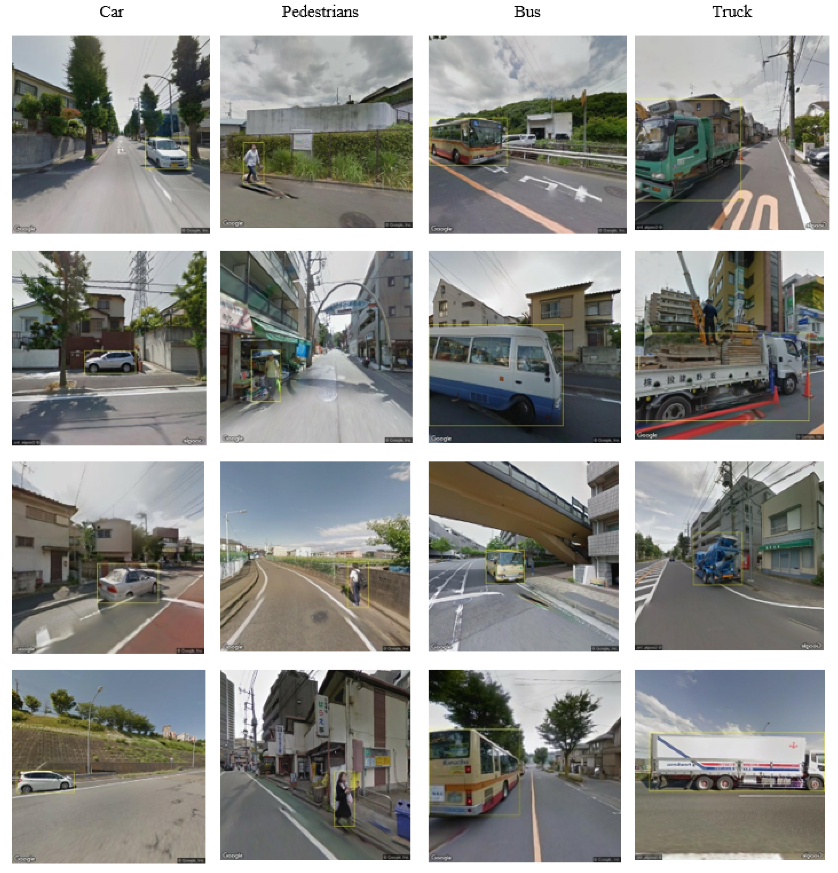
This dataset consists of a massive amount of images of eight defined classes of transport objects that vary widely in appearance, scale, occlusion and viewpoint. In particular, the target categories of road users include cars, pedestrians, buses, trucks, motor, vans, cyclists and parked cycles. This is implemented by reviewing the common transport modes that frequently appear in Tokyo. Single instances of road users are annotated individually. An excerpt of eight transport mode samples is illustrated in Figure 2. To reflect the complexity of this newly introduced dataset, the basic properties of TMS-Tokyo are listed in Table 1, together with those of other more established transport datasets, including the Tsinghua–Daimler Cyclist Benchmark [53], KITTI [56], Mapillary Vistas [60], BDD100K [61] and CityScapes [57]. Note that, whilst TMS-Tokyo is not the largest image dataset for object detection, it is the Google Street View dataset of the largest size which is specifically devised for transport object detection. Please refer to Appendix A and Appendix B for further details of the creation of the TMS-Tokyo Dataset.
4. Proposed Approach
This section presents a novel approach for the development of decomposed CNN-based transport object detection in street view imagery.
4.1. Data Augmentation
For street view imagery, the backgrounds of street views can be various and complicated associated with different locations and scenes. Road users often appear in different orientations, positions, scaling, and brightness. In practice, it is easy to fall into the trap of overfitting with limited data in the face of trillions of parameters in a deep neural network. The data augmentation technique helps increase the relevance of the data, minimizing the possibility of the neural networks learning irrelevant features, thereby radically improving overall performance.
An interesting approach for data augmentation is the Mosaic method first proposed in YOLOv4 [62], the main idea of which is to randomly crop a small number (four in a typical implementation) of images and to stitch them onto one image as training data. This paper adopts the Mosaic data augmentation technique on the dataset TMS-Tokyo, while turning off this operation in a number (say, 15) of the last epochs of training to prevent the images generated by data enhancement from interfering with the real distribution of natural images. An instance of the use of Mosaic in TMS-Tokyo is illustrated in Figure 3.
4.2. Dilated Convolution
Dilated convolution, widely employed in visual tasks, addresses the significant issue of local information loss caused by downsampling in semantic segmentation. The introduction of the DeepLab algorithm [63] demonstrates that, while simultaneously enlarging the receptive field, replacing pooling with dilated convolution allows each convolutional operation to encompass a larger range of relevant information within a fixed parameter count. The receptive field defines the size of the region in the input feature map where convolutional computations are performed, and the results obtained from this region correspond to a single point in the output feature map. Therefore, a larger receptive field contains more abundant contextual information from the original image, which is advantageous for improving model accuracy.
Dilated convolution introduces an expansion rate that indicates the spacing between parameters in the convolutional kernel. It allows for an enlarged receptive field without affecting the number of parameters, which remain unchanged. The calculation formula for the receptive field is
where represents the receptive field of the current layer, indicates the receptive field of the previous layer, denotes the stride of the convolutional or pooling layer, and k is the kernel size.
The effectiveness of dilated convolution is manifested in two respects. The primary means is its ability to expand the receptive field. While regular convolutions reduce spatial resolution through downsampling, dilated convolution maintains good spatial resolution to ensure accurate target localization, which is beneficial for detecting large objects. The other way that dilated convolution represents an advance is its capability of obtaining contextually relevant information at multiple scales. By adjusting the dilation rate, different receptive field sizes can be achieved, thereby obtaining diverse information at different scales. This method greatly aids visual tasks by providing information from different and multiple scales.
4.3. Tensor Train Decomposition
Tensor train (TT) decomposition is based on the matrix product state (MPS) model, which decomposes the input tensor into a series of adjacent three-dimensional and two-dimensional tensors. Typically, TT decomposition can be achieved by (N − 1) times singular value decomposition. For a fourth-order tensor, for instance, the decomposition takes the following form:
Figure 4 depicts a schema of the TT decomposition of a fourth-order tensor. The indices of the large tensor are denoted as , and each subsequent decomposition involves second- or third-order tensors with the first index corresponding to the original index of the large tensor. New auxiliary indices are introduced to facilitate the decomposition process. Consequently, the first sub-tensor resulting from the decomposition contains only one auxiliary index , while the second sub-tensor has two auxiliary indices and . This indicates that both ends of the decomposition are second-order tensors, while the intermediate tensor is a third-order tensor.
For a d-th order tensor , its Tucker decomposition is defined as follows: it decomposes each dimension into three-mode tensors, referred to as factors or cores. One dimension of the sub-tensor corresponds to the actual physical dimension, while the other two dimensions connect the preceding and succeeding cores.
Mathematically, the Tucker decomposition of the tensor is expressed as:
The process of an algorithm implementing such a schema can be divided into four steps, as follows:
- Step 1. Decomposing the convolutional kernel in the original neural network into a fourth-order core tensor, producing a factor matrix by TT decomposition.
- Step 2. Completing the factor matrix of the decomposition and filling the convolutional kernel parameters.
- Step 3. Assigning the new convolutional kernel parameters to the new convolutional kernel.
- Step 4. Replacing the original convolution kernel with the new two-layer mini-convolution.
The advantage of TT decomposition is that it is linear in relation to the number of entries (and, hence, storage) and computation time, enabling higher-dimensional problems to be addressed. In particular, when dealing with matrices, TT decomposition is equivalent to the singular value decomposition.
Finding the optimal rank is a key issue when compressing the model through low rank decomposition. Rank is the only hyperparameter that controls the computational complexity and accuracy in compressed convolutional neural networks. An excessively large rank clearly does not achieve maximum compression, whilst a rank that is too small may make accuracy recovery problematic. Instead of choosing the rank by time-consuming iterative trials, the empirical variational Bayes matrix factorization (EVBMF) [64] method is employed to automatically compute the rank.
In this work, a superior selection procedure is shown to be attainable for full variational Bayes matrix factorization (VBMF). More specifically, the global optimum is a re-weighted SVD of the observation matrix, and each weight can be obtained by solving a quadratic equation whose coefficients are a function of the observed singular values. Therefore, EVBMF, where the hyperparameters are learned from the data, is adopted in the present work to achieve the global optimal solution.
4.4. Algorithm Structure
4.4.1. Algorithm Details
In this study, the SVDet architecture is adopted with ResNet-50 as the backbone, fpn-neck, and RetinaHead. Tensor decompositions are performed separately on these components to investigate the effectiveness of low-rank decomposition in different parts (Algorithm 1).
| Algorithm 1 Illustration of Algorithm SVDet |
|
When applying low-rank decomposition to compress a model, finding the optimal rank is crucial, as it controls the trade-off between computational complexity and accuracy in compressed convolutional neural networks. Selecting an excessively large rank may fail to achieve maximal compression, while choosing too small a rank can hinder accuracy recovery. To address this, time-consuming trial-and-error approaches are avoided for rank selection. Instead, empirical variational Bayes matrix factorization (EVBMF) [64] is employed to compute the rank. In this work, a novel and superior alternative is used that exploits completely positive (CP)-like decomposition with variational Bayesian matrix factorization (VBMF) for the fully observed case, where the global solution can be analytically calculated. Specifically, the global solution involves the weighted SVD of the observation matrix, and each weight can be obtained by solving a quadratic equation with coefficients derived from the observed singular values. The detailed procedure for rank determination is presented in the following Section.
The TT decomposition methods are applied as described in the previous section to decompose the convolutional layers, reducing the number of parameters and allowing the replacement of the original tensors. To restore accuracy after model acceleration and compression while preserving the effectiveness of the model components, fine-tuning is performed on the dataset. This process results in a smaller yet more accurate model.
4.4.2. Rank Determination
As mentioned above, variational Bayesian matrix factorization (VBMF) is employed to compute the ranks used in low-rank decomposition for each of the convolutional kernel’s parameters.
The process of obtaining the rank for a four-order tensor, i.e., the calculation process of EVBMF, is illustrated in Figure 5. For tensor-train decomposition, the maximum rank is selected from and , since only one rank is required as the tensor rank. Choosing the maximum rank ensures accuracy and recoverability. Note that opting for a rank lower than the maximum increases the likelihood of compressing one or more dimensions excessively, which may lead to precision loss or irrecoverable issues.
4.5. Overall Structure of SVDet
Recall the original design intention, which is to develop a compact and high-precision model for traffic object detection in urban areas. Considering the objective of dealing with (and, hence, combining the metrics of) both detection accuracy and model complexity, the RetinaNet model is chosen as the baseline detector to perform low-rank decomposition in an effort to obtain a compact model. In implementation, SVDet consists of two steps: first decomposing and replacing the convolutional kernels (network weights) of the backbone and head parts of RetinaNet using the TT decomposition algorithm, and then fine-tuning the compressed model to reduce the impact of the decomposition on the resulting model accuracy.
Table 2 presents the statistics for the computational and parametric quantities for the backbone, neck and head parts of RetinaNet with Mosaic data augmentation. It can be seen that the backbone, as the feature extraction part of the detection model, accounts for a relatively large amount of computation and number of parameters, and the number of parameters accounts for 64.2% of the entire model. The head part is detected on multiple feature layers and its parameters are shared across these feature layers, so that the number of parameters in it is low though involving greater computation, reaching 51.1% of the entire model. In this paper, low-rank decomposition is performed on these two components. The overall algorithm structure of the low-rank decomposition of the backbone network of SVDet using the TT decomposition is shown in Figure 6.
5. Experimental Results and Analysis
The performance of SVDet was examined in comparison with other baselines on the TMS-Tokyo Dataset in accomplishing the task of multi-class transport object detection. The algorithm benchmarks employed are state-of-the-art deep CNN methods with proven superior performance and popularity when applied for object detection, including ResNet-50 and ResNet-101-based RetinaNet [17], Faster RCNN [32], Cascade RCNN [39], FCOS [43], and Darknet-based YOLOv3 [35].
5.1. Implementation Configuration
All experiments reported in the paper were performed on a 64-bit Ubuntu 18.04 operating system. The hardware was a GTX 1080 Ti GPU with 12 GB of RAM and a 10-core Intel(R) Xeon(R) CPUE5-2640 [email protected] GHz CPU with 32 GB of RAM. The entire dataset used for the experimental investigation was divided into three sets of training, validation and testing according to the ratio of 6:2:2. In presenting the following results, the unit of FLOPs is GFLPOs (1 GFLOPs = 109 FLOPs) and that of Params is megabytes (M).
5.2. Comparative Results
The results of the proposed SVDet were compared with those achieved by the other object detectors investigated on the TMS-Tokyo Dataset, as listed in Table 3. Judged by the mean average precision (mAP), SVDet outperformed the others. Through its balanced design, SVDet achieved 77.6% on mAP with ResNet-50. In particular, as a lightweight single-stage object detection method, SVDet significantly outperformed both typical one-stage and two-stage methods in terms of computational parameters. From the perspective of overall efficiency and effectiveness, SVDet was shown to be the most promising transport object detector.
5.3. Ablation Studies
For ablation experiments, the SVDet model trained on TMS-Tokyo served as the pretrained model for network initialization. In so doing, all model parameters were distributed in a performance-strong range at the beginning of training, alleviating potential overfitting while speeding up the convergence of the underlying model. RetinaNet was taken as the baseline due to its promising performance among classical detectors. To validate the design of the proposed model, experiments were conducted to test the influence of different model compression methods and that of low-rank decomposition of different modules, regarding the model performance and the number of computational parameters involved, respectively.
5.3.1. Comparison with Alternative Model Compression Algorithms
Comparative experimental tests were carried out against the baseline algorithm and three other classical model compression algorithms, namely CP decomposition, Tucker decomposition and stripe-wise pruning.
The results as given in Table 4 show that, while the other three methods experienced accuracy loss, SVDet (with TT decomposition) gained higher accuracy instead. In particular, in terms of computational and parametric quantities, CP decomposition reduced the maximum complexity but its accuracy significantly fell behind the rest. Furthermore, SVDet was demonstrated to be a low-rank decomposition that could balance the accuracy loss and computational parametric reduction, beating all the tested existing model compression algorithms.
5.3.2. Influence of Decompositions on Different Model Modules
To investigate the impact of the decomposition of different modules upon model performance and computational efficiency, a number of experiments were devised to decompose different components of the baseline algorithm using three low-rank decompositions. Each was initialized with the parameters of a pretrained model, noting that SVDet simultaneously performs a low-rank TT decomposition of both backbone and head modules for the baseline.
From the results of Table 5, it can be seen that the TT decomposition of the backbone and head of the baseline method provided the most promising outcomes. The approach introduced in this work only requires less than one-half of the number of parameters and of computation of the uncompressed model, while the accuracy gains a little over the uncompressed model.
Amongst the three components implemented for object detection, the maximum gain is achieved when performing low-rank decomposition on both the backbone and the head, because these components own the majority of the entire model parameters. Tucker decomposition is better than CP decomposition, but both of them have limitations: the former requires more storage space and lacks correlation information between any two patterns, while the latter lacks correlation information between the tensor and the other different patterns that Tucker decomposition can obtain. However, the tensor train (TT) decomposition shows a strong higher-order processing capability and is well suited for the decomposition of neural network models. This is feasible because SVDet is of a fourth-order tensor, with TT having a great advantage for the third-order and above.
5.3.3. Discussion of Comparative Experiments
Regarding the three components of object detection, the greatest gain was achieved when low-rank decomposition was performed simultaneously on the backbone and head. This is because the backbone constitutes 64.2% of the model’s parameters, while the head accounts for 51.1% of the model’s computational load. In tensor decomposition, Tucker and CP are commonly used, but Tucker, which can capture and reflect intermodal information, is more streamlined than CP. Therefore, the performance of Tucker decomposition is superior to CP decomposition. However, both methods have limitations: Tucker decomposition requires a large storage space and lacks information on the correlation between any two modes, whereas CP decomposition lacks the tensor and intermodal correlations that can be obtained through Tucker decomposition.
Applying generally to fourth-order tensors, tensor train (TT) decomposition exhibits strong high-order processing capabilities, making it highly suitable for neural network model decomposition. Indeed, TT has significant advantages for third-order tensors and above. The experiments conducted in this study demonstrated that TT decomposition can achieve quality model compression while maintaining a remarkable level of accuracy.
6. Conclusions
This paper has presented an innovative approach using deep learning to detect transport objects from Google Street View imagery in urban areas. A GSV imagery dataset (named TMS-Tokyo) has been introduced for the first time, involving eight categories of road users and containing 50,827 instances and 32,555 images. It is the largest Google Street View dataset specially designed for transport object detection. Further to the introduction of a new dataset, low-rank tensor decomposition has been proposed to compress the street view object detector from the perspective of compression parameters in order to tackle the challenging problems of high computational cost and parametric volume concerning the detection model. The resulting system SVDet applies tensor train decomposition to both the backbone and the head of the underlying model. It is able to achieve a mAP value of 77.6% on TMS-Tokyo, with a parametric number of 17.29 M and a computational volume of 16.52 G FLOPs, significantly outperforming state-of-the-art methods described in the literature. Thanks to such a lightweight design based on low-rank tensor decomposition, the approach developed herein helps address the important issue of environmental sustainability.
Whilst promising, opportunities arise for further development of the present work. In particular, to reflect and adapt to evolving urban transport conditions, TMS-Tokyo needs to be continuously updated and extended in both size and scope, by involving more cities on a global scale. How this system may be further developed to cope with the dynamically changing TMS-Tokyo dataset continues to be actively researched.
Author Contributions
Conceptualisation, Y.B. and Y.L.; methodology, Y.B.; software, Y.B.; validation, C.S., Y.L. and Q.S.; formal analysis, Y.B., L.S. and S.J.; investigation, C.S., L.S. and S.J.; resources, Y.L. and S.J.; data curation, Y.L. and Y.B.; writing—original draft preparation, Y.B.; writing—review and editing, C.S., Q.S. and Y.L.; visualization, Y.B.; supervision, C.S. and Q.S.; project administration, Y.B., Y.L. and Q.S.; funding acquisition, C.S. and Q.S. All authors have read and agreed to the published version of the manuscript.
Funding
This research received no external funding.
Data Availability Statement
The data presented in this study are available on request from the corresponding author. The data are not publicly available due to unforeseen circumstances.
Acknowledgments
The authors are grateful to the anonymous reviewers for their helpful comments to the conference paper (which received the Best Student Paper award) upon which the present work is developed. The first author is supported with a full International PhD Scholarship awarded by Aberystwyth University.
Conflicts of Interest
The authors declare no conflict of interest. The funders had no role in the design of the study; in the collection, analyses, or interpretation of data; in the writing of the manuscript; or in the decision to publish the results.
Abbreviations
The following abbreviations are used in this manuscript:
| MDPI | Multidisciplinary Digital Publishing Institute |
| DOAJ | Directory of Open Access Journals |
| TLA | three letter acronym |
| LD | linear dichroism |
| GSV | Google Street View |
| mAP | mean average precision |
| MPS | matrix product state |
| EVBMF | empirical variational Bayes matrix factorization |
| Params | parameters |
| FLOPs | floating point operations per second |
| CP | CANDECOMP/PARAFAC |
| TT | tensor train |
Appendix A. TMS-Tokyo Dataset
Appendix A.1. Dataset Category
In order to present the data on travel patterns, different types of road users are classified by observing street view images of Tokyo. When dividing the categories, parked cycles are separated from cyclists because parked cycles in the Tokyo dataset have a significant weight in the Google Street View Imagery of Tokyo. However, there is no division in the category of motorcycles vs. motorcyclists. The distinction between parked cycles and moving cycles is quite clear from the images as the location is used to differentiate between these two categories. This approach follows previous studies and includes two different categories for cycles as shown in Figure A1.
Figure A1.
(a) Parked cycles can be hard to label, (b) truck is occluded by another truck, (c) car occlusion.
Figure A1.
(a) Parked cycles can be hard to label, (b) truck is occluded by another truck, (c) car occlusion.

In contrast to Goel’s study [14], a distinction is herein made for vehicles that are classified for commercial use; vans and trucks are defined as two different categories as they have distinct appearances for an automatic detector. Usually, vans are significantly larger in width and height than ordinary cars, plus there is no protruding warehouse body before and after. However, trucks normally share protruding warehouse bodies and they visually differ from other vehicles. In total, eight categories of road users are used for later annotation: cars, pedestrians, buses, trucks, motors, vans, cyclists and parked bicycles.
Appendix A.2. Annotation Method
Different approaches to annotating are considered for this dataset. The commonly used technique in computer vision is bounding box annotation, which is used to annotate various visual concepts, such as objects and attributes [66]. A bounding box is normally described as , where indicates the centre location of the image, and w and h represent the width and heights of the bounding box in the picture coordinate system, respectively. Horizontal bounding boxes are more adequate for objects without various orientations compared with oriented bounding boxes. For transport objects from street view, target objects are perpendicular to the street ground from the observation, which matches with the horizontal bounding boxes.
To facilitate image observations and the accuracy of annotations, a Cloud document is created with eight representative images of all target objects, illustrating different samples of target categories for later annotation work. The data annotation work is divided amongst eight research assistants, each taught to identify and annotate images with a horizontal bounding box by labelme through sharing Cloud documentation for reference [14]. Further, samples are randomly picked from each resultant JSON file and are reassessed accordingly. Using this approach, their quality is assured in terms of the accuracy of annotations and classifications. An excerpt of the eight illustrated transport mode samples is shown in Figure A2.
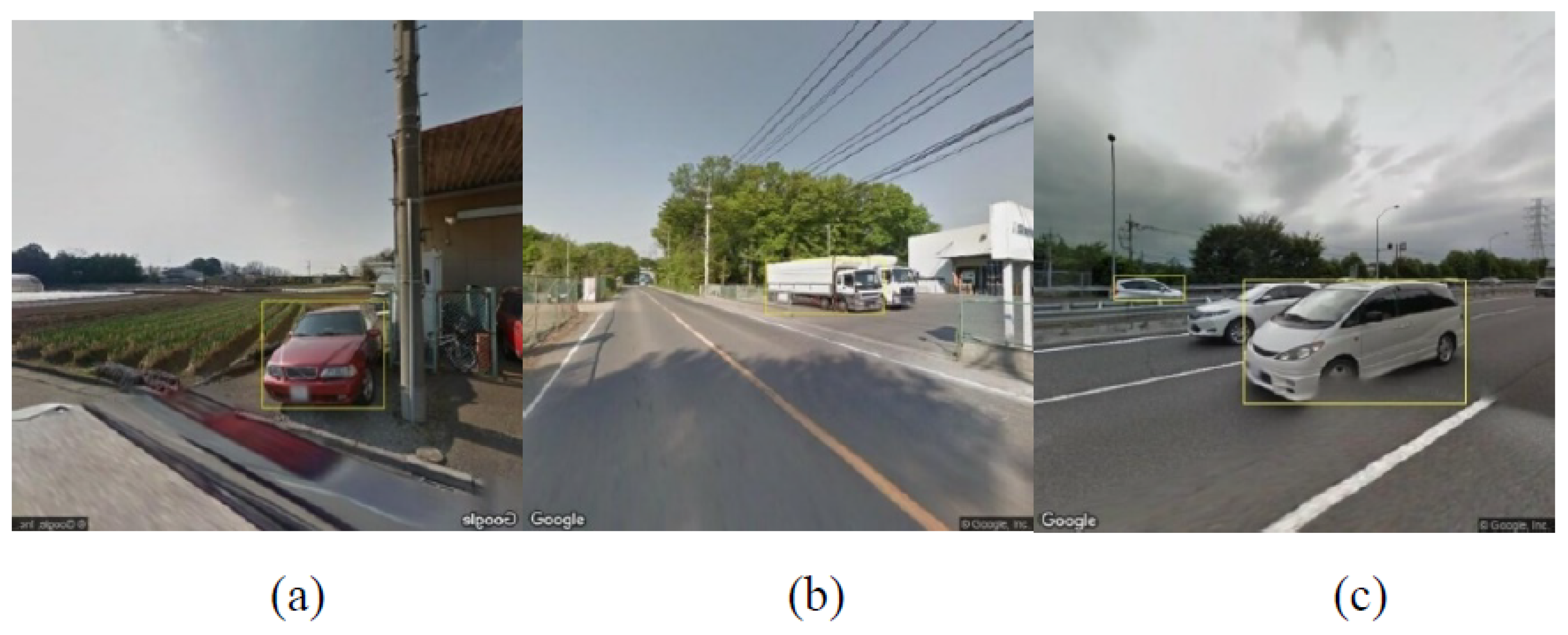
In contrast to aerial images, natural street-view images contain several instances at most. For Google Street View imagery of Tokyo, TMS-Tokyo contains at most ten instances per image. Therefore, it is not common to see areas densely crowded with instances compared with dense datasets [66]. Based on the demands of transport object counting, instances are annotated individually to distinguish them from other instances in the image. However, there are cases where transport objects are hard to label due to occlusions or their tiny size. Very difficult situations in noisy situations with significant occlusions are (reasonably) filtered.
Figure A2.
Excerpt of eight illustrated transport mode samples with annotations.

Appendix B. Variation of Transport Mode Shares by Region
The establishment of transportation modes depends mainly on the size and density of the population and that of the land, as well as the level of socio-economic development in the city concerned [12]. Cities or regions with relatively large population size and high population density emphasize the development of high-capacity public transportation (including rail transit, rapid transit, and other modes of transportation). In addition, transport policy will also influence people’s choice of transport modes.
The travel pattern is the structure of the traffic mode formed under the specific conditions of land layout, population density, economic level and social environment. This means a proportional distribution of the number of trips undertaken by the various modes of transport. Hence, the transport mode share varies in different countries or regions due to customs, culture, policies and geographic conditions [67]. Influenced by external factors, the dataset categories introduced in this work may not be able to adequately cover the urban transport mode shares of other countries or regions. As different cities may share different backgrounds or detection environment, the detection results of the learning frameworks might vary as well. Therefore, any application of the present approach to other cities will require careful empirical analysis of the local situation and associated detection validation.
References
- Diwan, T.; Anirudh, G.; Tembhurne, J.V. Object detection using YOLO: Challenges, architectural successors, datasets and applications. Multimed. Tools Appl. 2023, 82, 9243–9275. [Google Scholar] [CrossRef]
- Kaur, J.; Singh, W. Tools, techniques, datasets and application areas for object detection in an image: A review. Multimed. Tools Appl. 2022, 81, 38297–38351. [Google Scholar] [CrossRef] [PubMed]
- Bai, Z.; Wu, G.; Qi, X.; Liu, Y.; Oguchi, K.; Barth, M.J. Infrastructure-based object detection and tracking for cooperative driving automation: A survey. In Proceedings of the 2022 IEEE Intelligent Vehicles Symposium (IV), Aachen, Germany, 4–9 June 2022; pp. 1366–1373. [Google Scholar]
- Liang, S.; Wu, H.; Zhen, L.; Hua, Q.; Garg, S.; Kaddoum, G.; Hassan, M.M.; Yu, K. Edge YOLO: Real-time intelligent object detection system based on edge-cloud cooperation in autonomous vehicles. IEEE Trans. Intell. Transp. Syst. 2022, 23, 25345–25360. [Google Scholar] [CrossRef]
- Huang, Y.; Chen, J.; Huang, D. UFPMP-Det: Toward accurate and efficient object detection on drone imagery. In Proceedings of the AAAI Conference on Artificial Intelligence, Online, 22 February–1 March 2022; Volume 36, pp. 1026–1033. [Google Scholar]
- Mahaur, B.; Singh, N.; Mishra, K. Road object detection: A comparative study of deep learning-based algorithms. Multimed. Tools Appl. 2022, 81, 14247–14282. [Google Scholar] [CrossRef]
- Zhou, L.; Rao, X.; Li, Y.; Zuo, X.; Qiao, B.; Lin, Y. A lightweight object detection method in aerial images based on dense feature fusion path aggregation network. ISPRS Int. J. Geo-Inf. 2022, 11, 189. [Google Scholar] [CrossRef]
- Yang, Y.; Sun, X.; Diao, W.; Li, H.; Wu, Y.; Li, X.; Fu, K. Adaptive knowledge distillation for lightweight remote sensing object detectors optimizing. IEEE Trans. Geosci. Remote Sens. 2022, 60, 1–15. [Google Scholar] [CrossRef]
- Bi, R.; Xiong, J.; Tian, Y.; Li, Q.; Choo, K.K.R. Achieving lightweight and privacy-preserving object detection for connected autonomous vehicles. IEEE Internet Things J. 2022, 10, 2314–2329. [Google Scholar] [CrossRef]
- Liang, T.; Bao, H.; Pan, W.; Pan, F. ALODAD: An anchor-free lightweight object detector for autonomous driving. IEEE Access 2022, 10, 40701–40714. [Google Scholar] [CrossRef]
- Wu, P.; Liu, A.; Fu, J.; Ye, X.; Zhao, Y. Autonomous surface crack identification of concrete structures based on an improved one-stage object detection algorithm. Eng. Struct. 2022, 272, 114962. [Google Scholar] [CrossRef]
- Mueller, N.; Rojas-Rueda, D.; Basagaña, X.; Cirach, M.; Cole-Hunter, T.; Dadvand, P.; Donaire-Gonzalez, D.; Foraster, M.; Gascon, M.; Martinez, D.; et al. Health impacts related to urban and transport planning: A burden of disease assessment. Environ. Int. 2017, 107, 243–257. [Google Scholar] [CrossRef]
- Grimsrud, M.; El-Geneidy, A. Transit to eternal youth: Lifecycle and generational trends in Greater Montreal public transport mode share. Transportation 2014, 41, 1–19. [Google Scholar] [CrossRef]
- Goel, R.; Garcia, L.M.; Goodman, A.; Johnson, R.; Aldred, R.; Murugesan, M.; Brage, S.; Bhalla, K.; Woodcock, J. Estimating city-level travel patterns using street imagery: A case study of using Google Street View in Britain. PLoS ONE 2018, 13, e0196521. [Google Scholar] [CrossRef]
- Shi, T.; Ruth, M.; Townsend, A. Parallel algorithms for computing the tensor-train decomposition. SIAM J. Sci. Comput. 2023, 45, C101–C130. [Google Scholar] [CrossRef]
- Li, L.; Yu, W.; Batselier, K. Faster tensor train decomposition for sparse data. J. Comput. Appl. Math. 2022, 405, 113972. [Google Scholar] [CrossRef]
- Lin, T.Y.; Goyal, P.; Girshick, R.; He, K.; Dollár, P. Focal loss for dense object detection. In Proceedings of the IEEE International Conference on Computer Vision, Venice, Italy, 22–29 October 2017; pp. 2980–2988. [Google Scholar]
- Kalchbrenner, N.; Grefenstette, E.; Blunsom, P. A convolutional neural network for modelling sentences. arXiv 2014, arXiv:1404.2188. [Google Scholar]
- Wang, Z.J.; Turko, R.; Shaikh, O.; Park, H.; Das, N.; Hohman, F.; Kahng, M.; Chau, D.H.P. CNN explainer: Learning convolutional neural networks with interactive visualization. IEEE Trans. Vis. Comput. Graph. 2020, 27, 1396–1406. [Google Scholar] [CrossRef]
- Krizhevsky, A.; Sutskever, I.; Hinton, G.E. Imagenet classification with deep convolutional neural networks. Adv. Neural Inf. Process. Syst. 2012, 25, 1097–1105. [Google Scholar] [CrossRef]
- Deng, J.; Dong, W.; Socher, R.; Li, L.J.; Li, K.; Fei-Fei, L. Imagenet: A large-scale hierarchical image database. In Proceedings of the 2009 IEEE Conference on Computer Vision and Pattern Recognition, Miami, FL, USA, 20–25 June 2009; pp. 248–255. [Google Scholar]
- Alom, M.Z.; Taha, T.M.; Yakopcic, C.; Westberg, S.; Sidike, P.; Nasrin, M.S.; Van Esesn, B.C.; Awwal, A.A.S.; Asari, V.K. The history began from alexnet: A comprehensive survey on deep learning approaches. arXiv 2018, arXiv:1803.01164. [Google Scholar]
- He, K.; Zhang, X.; Ren, S.; Sun, J. Deep residual learning for image recognition. In Proceedings of the IEEE Conference on Computer Vision and Pattern Recognition, Las Vegas, NV, USA, 27–30 June 2016; pp. 770–778. [Google Scholar]
- Simonyan, K.; Zisserman, A. Very deep convolutional networks for large-scale image recognition. arXiv 2014, arXiv:1409.1556. [Google Scholar]
- He, K.; Zhang, X.; Ren, S.; Sun, J. Spatial pyramid pooling in deep convolutional networks for visual recognition. IEEE Trans. Pattern Anal. Mach. Intell. 2015, 37, 1904–1916. [Google Scholar] [CrossRef]
- Huang, G.; Liu, Z.; Van Der Maaten, L.; Weinberger, K.Q. Densely connected convolutional networks. In Proceedings of the IEEE Conference on Computer Vision and Pattern Recognition, Honolulu, HI, USA, 21–26 July 2017; pp. 4700–4708. [Google Scholar]
- Lin, T.Y.; Dollár, P.; Girshick, R.; He, K.; Hariharan, B.; Belongie, S. Feature pyramid networks for object detection. In Proceedings of the IEEE Conference on Computer Vision and Pattern Recognition, Honolulu, HI, USA, 21–26 July 2017; pp. 2117–2125. [Google Scholar]
- Liu, S.; Qi, L.; Qin, H.; Shi, J.; Jia, J. Path aggregation network for instance segmentation. In Proceedings of the IEEE Conference on Computer Vision and Pattern Recognition, Salt Lake City, UT, USA, 18–22 June 2018; pp. 8759–8768. [Google Scholar]
- Tan, M.; Pang, R.; Le, Q.V. Efficientdet: Scalable and efficient object detection. In Proceedings of the IEEE/CVF Conference on Computer Vision and Pattern Recognition, Seattle, WA, USA, 14–19 June 2020; pp. 10781–10790. [Google Scholar]
- Ghiasi, G.; Lin, T.Y.; Le, Q.V. Nas-fpn: Learning scalable feature pyramid architecture for object detection. In Proceedings of the IEEE/CVF Conference on Computer Vision and Pattern Recognition, Long Beach, CA, USA, 16–20 June 2019; pp. 7036–7045. [Google Scholar]
- Girshick, R.; Donahue, J.; Darrell, T.; Malik, J. Rich feature hierarchies for accurate object detection and semantic segmentation. In Proceedings of the IEEE Conference on Computer Vision and Pattern Recognition, Columbus, OH, USA, 23–28 June 2014; pp. 580–587. [Google Scholar]
- Ren, S.; He, K.; Girshick, R.; Sun, J. Faster r-cnn: Towards real-time object detection with region proposal networks. Adv. Neural Inf. Process. Syst. 2015, 28, 91–99. [Google Scholar] [CrossRef] [PubMed]
- Dai, J.; Li, Y.; He, K.; Sun, J. R-fcn: Object detection via region-based fully convolutional networks. Adv. Neural Inf. Process. Syst. 2016, 29, 379–387. [Google Scholar]
- Pang, J.; Chen, K.; Shi, J.; Feng, H.; Ouyang, W.; Lin, D. Libra r-cnn: Towards balanced learning for object detection. In Proceedings of the IEEE/CVF Conference on Computer Vision and Pattern Recognition, Long Beach, CA, USA, 16–20 June 2019; pp. 821–830. [Google Scholar]
- Redmon, J.; Farhadi, A. Yolov3: An incremental improvement. arXiv 2018, arXiv:1804.02767. [Google Scholar]
- Liu, W.; Anguelov, D.; Erhan, D.; Szegedy, C.; Reed, S.; Fu, C.Y.; Berg, A.C. Ssd: Single shot multibox detector. In Proceedings of the Computer Vision–ECCV 2016: 14th European Conference, Amsterdam, The Netherlands, 11–14 October 2016; Proceedings, Part I 14. Springer: Cham, Switzerland, 2016; pp. 21–37. [Google Scholar]
- Zhang, H.; Wang, K.; Tian, Y.; Gou, C.; Wang, F.Y. MFR-CNN: Incorporating multi-scale features and global information for traffic object detection. IEEE Trans. Veh. Technol. 2018, 67, 8019–8030. [Google Scholar] [CrossRef]
- Uijlings, J.R.; Van De Sande, K.E.; Gevers, T.; Smeulders, A.W. Selective search for object recognition. Int. J. Comput. Vis. 2013, 104, 154–171. [Google Scholar] [CrossRef]
- Cai, Z.; Vasconcelos, N. Cascade r-cnn: Delving into high quality object detection. In Proceedings of the IEEE Conference on Computer Vision and Pattern Recognition, Salt Lake City, UT, USA, 18–22 June 2018; pp. 6154–6162. [Google Scholar]
- He, K.; Gkioxari, G.; Dollár, P.; Girshick, R. Mask r-cnn. In Proceedings of the IEEE International Conference on Computer Vision, Venice, Italy, 22–29 October 2017; pp. 2961–2969. [Google Scholar]
- Wu, Y.; Chen, Y.; Yuan, L.; Liu, Z.; Wang, L.; Li, H.; Fu, Y. Rethinking classification and localization for object detection. In Proceedings of the IEEE/CVF Conference on Computer Vision and Pattern Recognition, Seattle, WA, USA, 14–19 June 2020; pp. 10186–10195. [Google Scholar]
- Redmon, J.; Divvala, S.; Girshick, R.; Farhadi, A. You only look once: Unified, real-time object detection. In Proceedings of the IEEE Conference on Computer Vision and Pattern Recognition, Las Vegas, NV, USA, 27–30 June 2016; pp. 779–788. [Google Scholar]
- Tian, Z.; Shen, C.; Chen, H.; He, T. Fcos: Fully convolutional one-stage object detection. In Proceedings of the IEEE/CVF International Conference on Computer Vision, Long Beach, CA, USA, 16–20 June 2019; pp. 9627–9636. [Google Scholar]
- Rigamonti, R.; Sironi, A.; Lepetit, V.; Fua, P. Learning separable filters. In Proceedings of the IEEE Conference on Computer Vision and Pattern Recognition, Portland, OR, USA, 23–28 June 2013; pp. 2754–2761. [Google Scholar]
- Denton, E.L.; Zaremba, W.; Bruna, J.; LeCun, Y.; Fergus, R. Exploiting linear structure within convolutional networks for efficient evaluation. Adv. Neural Inf. Process. Syst. 2014, 27, 1269–1277. [Google Scholar]
- Jaderberg, M.; Vedaldi, A.; Zisserman, A. Speeding up convolutional neural networks with low rank expansions. arXiv 2014, arXiv:1405.3866. [Google Scholar]
- Lebedev, V.; Ganin, Y.; Rakhuba, M.; Oseledets, I.; Lempitsky, V. Speeding-up convolutional neural networks using fine-tuned cp-decomposition. arXiv 2014, arXiv:1412.6553. [Google Scholar]
- Tai, C.; Xiao, T.; Zhang, Y.; Wang, X. Convolutional neural networks with low-rank regularization. arXiv 2015, arXiv:1511.06067. [Google Scholar]
- Denil, M.; Shakibi, B.; Dinh, L.; Ranzato, M.; De Freitas, N. Predicting parameters in deep learning. Adv. Neural Inf. Process. Syst. 2013, 26, 2148–2156. [Google Scholar]
- Sainath, T.N.; Kingsbury, B.; Sindhwani, V.; Arisoy, E.; Ramabhadran, B. Low-rank matrix factorization for deep neural network training with high-dimensional output targets. In Proceedings of the 2013 IEEE International Conference on Acoustics, Speech and Signal Processing, Vancouver, BC, Canada, 26–31 May 2013; pp. 6655–6659. [Google Scholar]
- Lu, Y.; Kumar, A.; Zhai, S.; Cheng, Y.; Javidi, T.; Feris, R. Fully-adaptive feature sharing in multi-task networks with applications in person attribute classification. In Proceedings of the IEEE Conference on Computer Vision and Pattern Recognition, Honolulu, HI, USA, 21–26 July 2017; pp. 5334–5343. [Google Scholar]
- Oseledets, I.V. Tensor-train decomposition. SIAM J. Sci. Comput. 2011, 33, 2295–2317. [Google Scholar] [CrossRef]
- Li, X.; Flohr, F.; Yang, Y.; Xiong, H.; Braun, M.; Pan, S.; Li, K.; Gavrila, D.M. A new benchmark for vision-based cyclist detection. In Proceedings of the 2016 IEEE Intelligent Vehicles Symposium (IV), Gothenburg, Sweden, 19–22 June 2016; pp. 1028–1033. [Google Scholar]
- Lin, T.Y.; Maire, M.; Belongie, S.; Hays, J.; Perona, P.; Ramanan, D.; Dollár, P.; Zitnick, C.L. Microsoft coco: Common objects in context. In Proceedings of the Computer Vision–ECCV 2014: 13th European Conference, Zurich, Switzerland, 6–12 September 2014; Proceedings, Part V 13. Springer: Cham, Switzerland, 2014; pp. 740–755. [Google Scholar]
- Everingham, M.; Van Gool, L.; Williams, C.K.; Winn, J.; Zisserman, A. The pascal visual object classes (voc) challenge. Int. J. Comput. Vis. 2010, 88, 303–338. [Google Scholar] [CrossRef]
- Geiger, A.; Lenz, P.; Urtasun, R. Are we ready for autonomous driving? the kitti vision benchmark suite. In Proceedings of the 2012 IEEE Conference on Computer Vision and Pattern Recognition, Providence, RI, USA, 16–21 June 2012; pp. 3354–3361. [Google Scholar]
- Cordts, M.; Omran, M.; Ramos, S.; Rehfeld, T.; Enzweiler, M.; Benenson, R.; Franke, U.; Roth, S.; Schiele, B. The cityscapes dataset for semantic urban scene understanding. In Proceedings of the IEEE Conference on Computer Vision and Pattern Recognition, Las Vegas, NV, USA, 27–30 June 2016; pp. 3213–3223. [Google Scholar]
- Anguelov, D.; Dulong, C.; Filip, D.; Frueh, C.; Lafon, S.; Lyon, R.; Ogale, A.; Vincent, L.; Weaver, J. Google street view: Capturing the world at street level. Computer 2010, 43, 32–38. [Google Scholar] [CrossRef]
- Middel, A.; Lukasczyk, J.; Zakrzewski, S.; Arnold, M.; Maciejewski, R. Urban form and composition of street canyons: A human-centric big data and deep learning approach. Landsc. Urban Plan. 2019, 183, 122–132. [Google Scholar] [CrossRef]
- Neuhold, G.; Ollmann, T.; Rota Bulo, S.; Kontschieder, P. The mapillary vistas dataset for semantic understanding of street scenes. In Proceedings of the IEEE International Conference on Computer Vision, Venice, Italy, 22–29 October 2017; pp. 4990–4999. [Google Scholar]
- Yu, F.; Chen, H.; Wang, X.; Xian, W.; Chen, Y.; Liu, F.; Madhavan, V.; Darrell, T. Bdd100k: A diverse driving dataset for heterogeneous multitask learning. In Proceedings of the IEEE/CVF Conference on Computer Vision and Pattern Recognition, Seattle, WA, USA, 14–19 June 2020; pp. 2636–2645. [Google Scholar]
- Bochkovskiy, A.; Wang, C.Y.; Liao, H.Y.M. Yolov4: Optimal speed and accuracy of object detection. arXiv 2020, arXiv:2004.10934. [Google Scholar]
- Chen, L.C.; Papandreou, G.; Kokkinos, I.; Murphy, K.; Yuille, A.L. Deeplab: Semantic image segmentation with deep convolutional nets, atrous convolution, and fully connected crfs. IEEE Trans. Pattern Anal. Mach. Intell. 2017, 40, 834–848. [Google Scholar] [CrossRef]
- Wang, W.; Stephens, M. Empirical bayes matrix factorization. J. Mach. Learn. Res. 2021, 22, 5332–5371. [Google Scholar]
- Zhang, S.; Chi, C.; Yao, Y.; Lei, Z.; Li, S.Z. Bridging the gap between anchor-based and anchor-free detection via adaptive training sample selection. In Proceedings of the IEEE/CVF Conference on Computer Vision and Pattern Recognition, Seattle, WA, USA, 14–19 June 2020; pp. 9759–9768. [Google Scholar]
- Xia, G.S.; Bai, X.; Ding, J.; Zhu, Z.; Belongie, S.; Luo, J.; Datcu, M.; Pelillo, M.; Zhang, L. DOTA: A large-scale dataset for object detection in aerial images. In Proceedings of the IEEE Conference on Computer Vision and Pattern Recognition, Salt Lake City, UT, USA, 18–22 June 2018; pp. 3974–3983. [Google Scholar]
- Oka, H.; Hagino, Y.; Kenmochi, T.; Tani, R.; Nishi, R.; Endo, K.; Fukuda, D. Predicting travel pattern changes of freight trucks in the Tokyo Metropolitan area based on the latest large-scale urban freight survey and route choice modeling. Transp. Res. Part E Logist. Transp. Rev. 2019, 129, 305–324. [Google Scholar] [CrossRef]
Figure 1.
Examples of CityScape’s fine annotations in high-quality dense pixels [57].
Figure 1.
Examples of CityScape’s fine annotations in high-quality dense pixels [57].

Figure 2.
Illustrative transport mode samples with annotations.


Figure 3.
Examples of Mosaic data augmentation: images (a–d) refer to four random images chosen for Mosaic data augmentation.
Figure 3.
Examples of Mosaic data augmentation: images (a–d) refer to four random images chosen for Mosaic data augmentation.

Figure 4.
Schematic representation of fourth-order tensor’s tensor train (TT) decomposition.

Figure 5.
Process for Rank Determination of Four-Order Tensor (Flowchart).

Figure 6.
Algorithm structure of SVDet, where red, blue and green dotted boxes indicate backbone, neck, and head part of SVDet, respectively.
Figure 6.
Algorithm structure of SVDet, where red, blue and green dotted boxes indicate backbone, neck, and head part of SVDet, respectively.


Table 1.
Properties of datasets.
| Dataset | Annotation | #Categories | #Instances | #Images |
|---|---|---|---|---|
| Tsinghua–Daimler Cyclist [53] | Horizontal BBox | 7 | 32,361 | 14,674 |
| Cityscapes [57] | Segmentation | 30 | NA | 25,000 |
| KITTI [56] | Segmenation | 5 | 80,256 | 14,999 |
| Mapillary Vistas [60] | Segmentation | 66 | >2 M | 25,000 |
| BDD 100K [61] | Horizontal BBox | 10 | 3.3 M | 100,000 |
| TMS-Tokyo | Horizontal BBox | 8 | 50,827 | 33,461 |
Table 2.
FLOPs and Params for different parts of baseline model.
| Parts | FLOPs (G) | Params (M) |
|---|---|---|
| Baseline | 53.07 | 36.25 |
| Backbone | 21.52 (40.6%) | 23.28 (64.2%) |
| Neck | 4.42 (8.3%) | 8.0 (22%) |
| Head | 27.13 (51.1%) | 4.97 (13.7%) |
Table 3.
Numerical experimental results on TMS-Tokyo Dataset.
| Methods | Backbone | mAP (%) | FLOPs (G) | Params (M) |
|---|---|---|---|---|
| Faster R-CNN [32] | R50 | 76.20 | 63.28 | 41.16 |
| R101 | 76.60 | 82.76 | 60.15 | |
| Cascade R-CNN [39] | R50 | 76.80 | 91.07 | 69.95 |
| R101 | 77.10 | 110.55 | 87.94 | |
| YOLOv3 [35] | Darknet | 76.10 | 49.66 | 61.56 |
| FCOS [43] | R50 | 74.50 | 50.41 | 31.85 |
| R101 | 75.60 | 69.88 | 50.79 | |
| RetinaNet [17] | R50 | 75.90 | 53.07 | 36.25 |
| R101 | 76.30 | 72.55 | 55.24 | |
| ATSS [65] | R50 | 75.30 | 51.63 | 31.90 |
| SVDet | R50 | 77.60 | 16.52 | 17.29 |
SVDet (shown in bold) indicates presently proposed model.
Table 4.
Comparison with other model compression algorithms.
| Methods | mAP (%) | FLOPs (G) | Params (M) |
|---|---|---|---|
| Baseline | 76.9 | 53.07 | 36.25 |
| Stripe-Wise Pruning | 72.37 (5.9%↓) | 31.31 (41.0%↓) | 18.85 (48.0%↓) |
| CP decomposition | 56.80 (26.1%↓) | 11.42 (78.5%↓) | 12.72 (64.9%↓) |
| Tucker decomposition | 68.20 (11.3%↓) | 15.21 (71.3%↓) | 14.68 (59.5%↓) |
| TT decomposition | 77.60 (0.9%↑) | 16.52 (68.9%↓) | 17.29 (52.3%↓) |
Table 5.
Comparison with existing model compression algorithms.
| Backbone | Head | mAP (%) | FLOPs (G) | Params (M) |
|---|---|---|---|---|
| × | × | 76.9 | 53.07 | 36.25 |
| ✓ | × | 78.10 (1.6%↑) | 41.43 (21.9%↓) | 21.85 (39.7%↓) |
| × | ✓ | 77.80 (1.2%↑) | 28.17 (46.9%↓) | 31.69 (12.6%↓) |
| ✓ | ✓ | 77.60 (0.9%↑) | 16.52 (68.9%↓) | 17.29 (52.3%↓) |
Disclaimer/Publisher’s Note: The statements, opinions and data contained in all publications are solely those of the individual author(s) and contributor(s) and not of MDPI and/or the editor(s). MDPI and/or the editor(s) disclaim responsibility for any injury to people or property resulting from any ideas, methods, instructions or products referred to in the content. |
© 2023 by the authors. Licensee MDPI, Basel, Switzerland. This article is an open access article distributed under the terms and conditions of the Creative Commons Attribution (CC BY) license (https://creativecommons.org/licenses/by/4.0/).
Share and Cite
MDPI and ACS Style
Bai, Y.; Shang, C.; Li, Y.; Shen, L.; Jin, S.; Shen, Q. Transport Object Detection in Street View Imagery Using Decomposed Convolutional Neural Networks. Mathematics 2023, 11, 3839. https://doi.org/10.3390/math11183839
AMA Style
Bai Y, Shang C, Li Y, Shen L, Jin S, Shen Q. Transport Object Detection in Street View Imagery Using Decomposed Convolutional Neural Networks. Mathematics. 2023; 11(18):3839. https://doi.org/10.3390/math11183839
Chicago/Turabian StyleBai, Yunpeng, Changjing Shang, Ying Li, Liang Shen, Shangzhu Jin, and Qiang Shen. 2023. "Transport Object Detection in Street View Imagery Using Decomposed Convolutional Neural Networks" Mathematics 11, no. 18: 3839. https://doi.org/10.3390/math11183839
Note that from the first issue of 2016, this journal uses article numbers instead of page numbers. See further details here.