1. Introduction
In the digital age, the importance of recommender systems has surged, driven by the growing consumer need for guidance in navigating through an abundance of options. A recommender system employs machine learning algorithms trained with actual data to identify evolving patterns in user behavior, subsequently leveraging this insight to present fresh recommendations to users [
1].
The extensive use of the Internet enables people to interact with social media, an essential part of our daily lives in the significant data world [
2]. Users can share opinions, ideas, and comments on various subjects, including news, locations, social events, and multimedia. Specifically, the movie domain represents a topic of interest due to its commercial value. This interest has fueled the growth of social media platforms, websites, and blogs, offering a space for both users and critics to express their opinions on any film created.
Gaining insights into how audiences perceive television programs and movies is a crucial aspect of the entertainment industry. For instance, movie production companies and investors often seek audience feedback for the films they support. Feedback from viewers can play a pivotal role in evaluating different elements, including the overall quality of a movie, the effectiveness of specific scenes, the impact of prevailing public opinion on the film’s success or failure, and recommendations for improving the movie. Additionally, this feedback can influence decisions related to future productions, such as casting choices for specific genres or selecting scenes to include in trailers to attract audiences. Ultimately, these considerations can lead to increased revenue for movie production companies.
Movie reviews are a valuable tool for users to assess and determine whether a specific film aligns with their preferences. Movie-related data, such as the extensive Internet Movie Database (IMDb), includes thousands of movie reviews. Nonetheless, manually scrutinizing each review can be an arduous and time-consuming task. Hence, integrating machine learning models offers a potential solution for efficiently automating and analyzing these reviews.
IMDb is one of the most popular online sites and databases for movies and TV shows. This platform provides a collection of datasets with significant information about films and shows, including information about the crew, cast, ratings, age classifications, categories, genres, reviews, and summaries [
3]. Accessible to anyone, this resource enables individuals to analyze the facets that intrigue them the most, whether the presented attributes are for box office hits or less successful productions.
Furthermore, part of this analysis relies on natural language processing (NLP) tools to gather information from user reviews and ratings. The IMDb dataset, featuring 50,000 reviews categorized as either positive or negative, is widely utilized for sentiment analysis, This dataset, developed by Mass et al. in 2011, employs NLP techniques, including semantic word similarities and a probabilistic model for word representation [
4].
Other popular datasets are “The movie dataset” by Rounak Banik [
5], principally containing rating and metadata but no text data information, and the “IMDb Dataset of 50K Movie Reviews” by Lakshmi Pathi [
6] which is composed of movie metadata and reviews from 50,000 movies.
Most of these datasets are not curated—the data are extracted, but the opinions may be diverse and unable to reflect the genre of the movie reviewed. This generates a problem when a class is misrepresented due to a lack of consistency or unbalanced data per class. These are common issues with short texts serving as opinions, and with most data scraped from the web, topics or classes might need to be labeled correctly, resulting in an imbalanced dataset [
7].
According to Unal et al. (2023) [
8], multilabel classification involves attributing multiple labels or tags to a given input instance. Within the specific domain of movie films, this task involves recognizing and allocating appropriate genre labels to posters based on their visual attributes. Film genres, such as action, romance, comedy, horror, sci-fi, and numerous others, encompass the diverse spectrum of cinematic offerings, each characterized by distinct visual elements and themes. The ability to automatically categorize movie films into multiple genres not only streamlines the process of cataloging and organizing but also unlocks opportunities for tailored recommendations, genre-focused marketing approaches, and enriched user interactions within cinema.
The goal of our proposed work is to establish a methodology for the reclassification of a sizable dataset acquired through web scraping. We note that the effectiveness of a machine learning model is directly influenced by the quality of the dataset used for training. The labels could be more reliable despite the extensive document volume of many large movie review datasets. Consequently, we embarked on creating our own extensive movie review dataset. Thus, we introduce a methodology for cleaning and categorizing text data. During our investigation, we rapidly recognized the significant impact of the stopword removal technique on text cluster formation and the embedding method. Thus, our focus was directed towards these two aspects.
The rest of the paper is structured as follows:
Section 2 comprehensively examines prior research on text classification techniques applied to movie reviews categorized by genre.
Section 3 outlines the approach and novel methods we have introduced for clustering and analyzing movie reviews.
Section 4 showcases the outcomes of our experiments, and the final section considers the key discoveries and conclusions drawn from our research.
2. Related Works
Although nowadays we have extensive access to information, we encounter new issues in the analysis and classification of this data. Although many machine learning models have been modeled and trained with datasets retrieved from different sources, we face challenges, such as the need for gold standards and annotated data [
9]. Therefore, classical text analytic techniques continue to form the foundation of numerous industrial applications.
2.1. Movie Classification by Genre
Movie reviews are readily available and accessible online. Moreover, movies are a popular form of entertainment, and people often seek out reviews to make informed decisions about what to watch. Therefore, it is unsurprising that the use of reviews has been revisited to create predictive models using different datasets.
Some of the first works, including movie summaries extracted from IMDb, were presented by Ka-Wing Ho (2011) [
10]. These works used a dataset of 16,000 unique movies categorized into 20 different and popular movie genres. Their model evaluation encompassed a range of models, including the support vector machine (SVM), K-nearest neighbors (KNN), and a simple neural network. Surprisingly, the SVM model emerged with the highest F-score among all the models, reaching 0.5499. Similarly, ref. [
11] created a multi-language dataset which extracted summaries from nearly 15,000 movies. They reduced 27 genres into nine broader genre classes. For instance, genres like action, adventure, sci-fi, sport, and war were manually labeled “action”. The models employed by them spanned regular machine learning models, like SVM and random forest (RF), as well as some more sophisticated neural network models, with the conclusion that the best model to classify movies by genre was a long short-term memory hybrid (LSTM-Hybrid) model with an accuracy above 89% for all the languages tested. During the same year, ref. [
12] explored various machine and deep learning techniques, using a corpus with up to 250,000 summaries from IMDb films, considering 20 different genres. After comparing several machine learning models, they found that the GRU model was optimal, delivering an F-score of 0.56. One recurring challenge with movie summary datasets is class imbalance. Genres like action or drama tend to include a substantial quantity of reviews. In contrast, genres such as western or war pose difficulties for detection by trained models, even when achieving high accuracy and F-scores [
10,
11,
12].
Recently, a more significant movie review dataset was released, containing nearly 1 million unique reviews from 1150 different IMDb movies, including metadata, and focusing on 17 genres. The high amount of data improved the overall machine and deep learning classification score. However, there was no information provided about performance by genre. Similar to other movie review datasets, genres like war or western have fewer entries compared to the most popular genres, such as action or drama [
13].
In the natural language processing field, a “gold standard” refers to a reference dataset or annotation considered the most reliable and accurate source of truth for a particular NLP task. Some examples include the Gold Standard corpus. Experts created and reviewed it to ensure proper data annotation in general text classification tasks [
14]. Several corpora for text classification, such as the AG’s news corpus [
15] and DBPedia [
16], are commonly employed for testing new machine learning classification algorithms. Nevertheless, a definitive gold standard for movie reviews and genre classification remains to be developed.
Creating and maintaining high-quality gold standards can be time-consuming and labor-intensive, as these often require human annotators to label the data. Hence, one approach to mitigate the risk of mislabeling or subpar annotations in extensive datasets is to turn to text clustering. Cluster analysis, an unsupervised technique, involves categorizing data instances into clusters that share substantial similarities without prior knowledge of the group structure or class labels [
17].
2.2. Clustering Approaches
In early 1939, the first clustering algorithms were developed due to the need to classify data. The social and biological sciences began searching for an automatized and organized approach to divide information into more approachable groups or clusters with similar characteristics. The first two identified algorithms were based on partitions and hierarchies [
18].
Nowadays, clustering algorithms have emerged as a powerful tool to accurately analyze the great amount of data generated by modern applications in a large variety of fields, such as biology [
19], medicine [
20], business and marketing [
21], the World Wide Web [
22], social science [
23], and computer science [
24].
The natural language processing approach involves grouping similar documents or sentences based on their content. Therefore, organizing large amounts of unlabeled or mislabeled text data into meaningful clusters is possible. As summarized by [
25], clustering algorithms can be divided into partitioning-based, hierarchical-based, density-based, grid-based, or model-based (see
Table 1).
Several clustering algorithms help to classify similar text documents together. The most crucial clustering algorithms are K-means [
26], K-medoids [
28], hierarchical-based [
46], and density-based [
38]. K-means and K-medoids are the most popular hard clustering algorithms [
47]. Both have proved to be suitable and adequate for natural language processing tasks.
Table 2 summarizes current works using clustering algorithms for text data classification.
Considering all these factors, we present an unsupervised movie review classification approach that involves various preprocessing techniques, including TF-IDF vectorization, Word2Vec embeddings, K-means clustering, and dimensionality reduction using principal component analysis (PCA). This method is applied to a movie review dataset from IMDb using the Python web scraping library Beautiful Soup. The overall goal is to design a methodology that allows proper cluster formation, with the primary purpose of genre identification. Cluster-annotated datasets are subjected to a similar machine-learning model to assess their accuracy, recall, precision, and F1-score differences.
3. Materials and Methods
As mentioned previously, the primary purpose of this paper is to develop a model for predicting movie genres using IMDb movie reviews.
Figure 1 presents the proposed general framework and the stages involved in the analysis.
3.1. Data Collection
To generate the dataset, Python web-scraping libraries were employed to extract movie details from the list of top IMDb movies belonging to 18 movie genres—action, adventure, animation, biography, comedy, crime, drama, fantasy, history, horror, music, mystery, romance, sci-fi, sport, thriller, war and western. Our process yielded a repository of up to 3.5 million unprocessed reviews, derived from 3688 unique movies using Python web-scraping libraries. Movies with fewer than 20 reviews were excluded from consideration. Moreover, we filtered out reviews containing fewer than 50 words or exceeding 500 words in length.
3.2. Text Preprocessing
The initial raw reviews were cleaned with preprocessing and noise reduction tools, principally those included in the Python library, NLTK [
61]. The text cleaning process involved the elimination of HTML tags, special characters, different short and long words, lemmatization, and stemming. Additionally, other lists were tested to remove stopwords, as depicted in
Figure 1. The lists employed were NLTK [
61], ISO project [
62], Genrec [
13], and custom-generated stop-lists with our proposed method.
3.2.1. Removal Methods for Stopwords
We present
Table 3, which summarizes the methods employed to remove stopwords. Our proposed method “Threshold” described in Algorithm 1 is divided into three main steps:
- (a)
Iterate the list of genres against the movie reviews to create a vocabulary without repeated words and the counter of each term for each genre.
- (b)
Iterate the vocabulary without repeated words against the list of genres, and if the word is in all the genres, then the word is added.
- (c)
Finally, a threshold is set (the minimum times a word must appear in each genre to be added). Iterate the vocabulary list in each genre against the list of genres. If the word is in all the genres and the word occurrences are equal or greater than the threshold, then the word is added.
With these steps, a list of stopwords is generated to be removed from the dataset.
| Algorithm 1. Threshold Method: Return Stopwords List |
- 1:
Input: - 2:
: The input DataFrame - 3:
: The list of genres - 4:
: Column name containing genres in the DataFrame - 5:
: Column name containing text data in the DataFrame - 6:
: The threshold for word frequency - 7:
: List of exceptions ▹ Used to skip words from result - 8:
Output: - 9:
: List of stopwords - 10:
function ReturnStopwordsList( , , , , , ) ▹ See Table 4 for - 11:
Initialize as an empty dictionary - 12:
Initialize as an empty set - 13:
Initialize as an empty list - 14:
Initialize as an empty list - 15:
Initialize as an empty list - 16:
for in do ▹ movie_detail: Each row of the dataframe - 17:
for in do - 18:
for in do - 19:
if not in then - 20:
- 21:
Increment the count of in - 22:
Add to the set - 23:
for in do - 24:
Set to True - 25:
Initialize to 0 - 26:
for in do - 27:
if not in then - 28:
Set to False - 29:
else - 30:
Increment by - 31:
if is True then - 32:
Add to - 33:
Add to - 34:
if is less than 1 then - 35:
Set to 1 - 36:
for in do - 37:
Set to True - 38:
for in do - 39:
if not in then - 40:
Set to False - 41:
break - 42:
else if then - 43:
Set to False - 44:
break - 45:
if is True and not in then - 46:
Add to - 47:
return
|
Table 3.
Removal methods for stopwords.
Table 3.
Removal methods for stopwords.
| Method | Description |
|---|
| Baseline | The study’s starting point is the initial dataset, which has been subjected to cleaning processes involving removing special characters, HTML tags, lemmatization, and stemming, while the stopwords have been retained. |
| Classic method: Precompiled stopwords lists | In this case, we employed three different precompiled stopwords lists: NLTK [61], ISO-en [62], and the list generated by [13] referred to as Genrec. |
| Method based on Zipf’s law: Z-Method | There are many different methods to compute custom stoplists for various languages. The most common ones are based on Zipf’s law [63]. This method calculates the frequency of each distinct word in the text, and then the words are sorted in decreasing order of their frequencies. So, the top k most frequent words are added to a stopword list and removed from the text. |
| Proposed method: Threshold | Our method verifies if a proposed stopword is present in each review across all genres. If this condition is satisfied, it examines whether the word’s frequency surpasses a specified threshold (see Algorithm 1). |
| Combined stopwords list | Datasets were cleaned with the list of stopwords mentioned above, and then with the Z-Method or the Threshold method or custom stopwords were detected and removed. |
3.2.2. TF-IDF Method
The term frequency–inverse document frequency (TF-IDF) is a numerical statistic that reflects a word’s importance to a document in a collection or corpus [
64]. TF-IDF is the product of two statistics: the term frequency and the inverse document frequency. Thus, the term frequency,
is the relative frequency of the term
t within a document
d. Moreover,
represents the raw count of a term in a document, i.e., the number of times that term
t occurs in a document
d.
On the other hand, the inverse document frequency measures how much information the word provides, whether it is a common word in all documents or a rare one. It is defined as the logarithmically scaled inverse fraction of the documents that contain the word (see Equation (
2)). Thus,
N denotes the total number of documents in the corpus
, and
is the number of documents in which the term
t appears.
Finally, Equation (
3) shows the combination of the two previous formulas. We use the term frequency–inverse document frequency:
3.2.3. Word2Vec Method
One problem with text classification is that the bag-of-words (BoW) feature and the conditional independence assumption need to be revised to capture the meaning of sentences in the text. Therefore, we employed rich contextual representations for words learned by the Word2Vec framework [
65]. Each review is turned into a vector representation by taking the average of the embedding vectors of all the words in each text. The assumption is that the average vector can be an excellent semantic summarization of the review.
3.2.4. K-Means Clustering
K-means clustering is the partitioning clustering method most frequently used in data mining; the algorithm segregates an N number of documents into a K number of clusters, while the value of K is specified by users or determined by methods such as elbows. Thus, the true K will be used to partition our N documents into K different classes in which documents of the same cluster must be similar and dissimilar from the other groups or classes using similarity formulas, like Euclidean or cosine similarity.
This clustering algorithm aims to decrease the summation of the square distance among data points and their respective cluster centers or centroids. The computing steps required for the K-means clustering method were defined by [
26]. Thus, selecting the initial
K cluster centers occurs as follows:
Now, to distribute the data
X in
K clusters at the
iteration, we used the following relation:
For all
;
; where
represents the set of data points whose cluster center is
. Calculate the new center
as the summation of the squared distances to the new cluster center from all points in
minimized. The part that works to reduce the distance is simply the mean of
. Thus, the new cluster center is computed as follows:
stands for the number of samples in , if for ; then the algorithm halts due to converged action, otherwise repeat the second step (5).
In this process, it is clear that the final clustering results are always affected by the initial seed and actual value of K. However, the initial seeds and the true value of K present in the dataset require previous knowledge, which is mostly impractical.
3.2.5. Mini-Batch K-Means
The mini-batch K-means algorithm was developed as a variant of the standard K-means clustering algorithm [
66]. Mini-batches are subsets of the input data, randomly sampled in each training iteration. These mini-batches drastically reduce the computation required to converge to a local solution. In contrast to other algorithms that reduce the convergence time, mini-batch K-means produces results that are generally only slightly worse than the standard algorithm. Therefore, it allows us to calculate common metrics to estimate the ideal number of clusters, like the inertia (elbow) method [
67], the silhouette score [
68], or the Calinski–Harabasz score [
69].
Thus, we decided to use the silhouette score as it gives good results in practice [
70]. The silhouette score is a reliable metric to predict the adequate number of clusters. Thus, we determined to use it to evaluate our datasets. Equation (
7) denotes the silhouette coefficient, where
a corresponds to each sample’s mean intra-cluster distance (
a) and the mean nearest-cluster distance (
b). The best value is 1, and the worst value is −1. Values near 0 indicate overlapping clusters.
The mini-batch K-means algorithm was employed for all datasets to predict the optimal cluster number. Once they were obtained, the standard K-means algorithm ran with each dataset’s predicted number of clusters.
3.3. Visualization Stage
All plots were generated with matplotlib.pyplot from Python version 3.11.4. Principal component analysis (PCA) was employed to represent the dimensionally reduced data. Statistical analysis was performed and annotated with Python library statannotations. For all column analysis, a t-test for independent samples was used to compare the groups.
3.4. Postprocessing Stage
In this stage, we performed text classification postprocessing, utilizing machine learning techniques to optimize the classification task.
Thus, we employed two of the most efficient classifiers from Sklearn to use as the base models. The data were divided into train and test datasets with a relation 8:2. The following subsections describe the methods that provided the better results in the case study.
3.4.1. Logistic Regression Approach
This is a statistical model that uses a logistic function to model a binary dependent variable (see Equation (
8)).
If the −z exponent tends to minus infinity, we have a minimum value close to 0. If the −z exponent tends to positive infinity, the value tends to 1. Values between 0 and 1 give us the probability of the function [
71]. Given the asymptotic nature of the logistic function, it can lead to a loss close to 0 when the dimensions are enormous. Therefore, most logistic models use regularization strategies, like L2, or reduce the number of cycles/epochs in training.
3.4.2. Support Vector Machine Approach
Support vector machine (SVM) is a supervised algorithm for classification and regression tasks. Support vector machine classifies the data by finding a hyperplane that maximizes the margin between the classes when training the data. In a two-dimensional example with two classes, we can think of the hyperplane as the line that separates the two classes [
72].
During the model performance, the separating hyperplane is one of the probable planes separating the two classes. SVM finds an optimal hyperplane by distinguishing the two classes, using Equation (
9) proposed by [
73].
Subject to the following constraints:
where
w is a coefficient vector,
b is the offset of the hyperplane from the beginning,
is the positive slack variable, and
c (≥0) signifies the penalty parameters of the errors.
3.4.3. Evaluation Metrics
Machine learning classifiers summarize the performance of each text classifier on the test dataset and evaluate the results into the following metrics: micro-average precision, micro-average recall, and micro-average F-score. The definition of these metrics is as stated in [
13].
where
represents the true positive values,
indicates the false negative values, and
describes the false positives after processing.
Moreover, to compute the prediction score of each text classifier method, we employed Equation (
15).
where
is the number of clusters defined as a genre and
C is the total number of clusters.
On the other hand, concerning the statistical analysis, data are the means plus standard deviation, calculated and annotated with the statannotations package version 0.6.0. A p-value < 0.05 is marked as significant.
4. Experimental Results
Using the Python web-scraping libraries, we retrieved up to 4 million reviews from IMDd, tagged with one to three genres each. The majority of reviews fell between ‘Drama’ and ‘Comedy’. We sought to balance this dataset to have a similar number of reviews by genre (see
Table 4).
Table 4.
Reviews per genre in the original dataset.
Table 4.
Reviews per genre in the original dataset.
| Genre | Reviews |
|---|
| Biography | 33,295 |
| History | 24,397 |
| Action | 28,723 |
| Drama | 36,565 |
| Horror | 20,477 |
| Comedy | 31,181 |
| Romance | 24,671 |
| Adventure | 25,048 |
| Crime | 24,557 |
| Mystery | 16,033 |
| Sci-Fi | 13,985 |
| Thriller | 23,646 |
| Fantasy | 13,982 |
| War | 19,111 |
| Music | 20,814 |
| Western | 19,293 |
| Sport | 18,129 |
| Animation | 24,530 |
| Total | 418,437 |
In addition, we produced 25 datasets cleaned with different stopword lists and vectorized either with TF-IDF or embedded with Word2Vec before clustering (see
Table 5). For each dataset, the ideal quantity of clusters was estimated and assessed by mini-batch K-means and silhouette scores. Each cluster’s top features were selected to evaluate whether they belonged to a specific movie genre.
First, we compared the effect of tokenization on the clustering performance (see
Figure 2). Generally, tokenization with TF-IDF (mean = 0.42 ± 0.11) resulted in higher silhouette scores than Word2Vec (mean = 0.24 ± 0.06). Here, we show an example of the scores generated by the process (see
Figure 3).
We also analyzed the effect of the tokenization on the estimation of the number of clusters with TF-IDF (mean = 12.42 ± 5.16) or Word2Vec (mean = 11.71 ± 4.84) (see
Figure 4). Moreover,
Figure 5 depicts an example of the clusters formed with TF-IDF or Word2Vec. Although the clusters might look fine, we did not find a significant difference regarding the top features in each cluster comparing TF-IDF (see
Table 6) against Word2Vec (
Table 7). TF-IDF text vectorization provided features easily relatable to movie genres, whereas Word2Vec repeated similar words across the different clusters.
Thus, the results resembled the effect of tokenization on the clustering time (see
Figure 6). Globally, the impact of the text vectorization method showed that TF-IDF (mean = 5784.33 s ± 2524.19 s) took more time than Word2Vec (mean = 4268.04 s ± 1213.17 s) or the clustering time taken by mini-batch K-means.
Furthermore, we were able to predict if a cluster could identify a specific movie genre by the top features in each cluster, similar to the previous results. Using TF-IDF (mean = 81.34 ± 20.48) before running the K-means clustering resulted in more identifiable genres than when Word2Vec was used (mean = 53.51 ± 24.1, see
Figure 7).
The balanced datasets improved the results when training a machine learning model [
74]. We tested our different datasets using a logistic regression model and a linear support vector machine approach.
Firstly, we noticed that similarly to clustering, metrics such as the precision, recall, F1-score, and Jaccard Index were higher when using the TF-IDF prior clustering algorithms with the logistic regression classifier (see
Figure 8). Due to our data distribution, we preferred the F1-score to the accuracy. The F1-score is especially suitable for our data because it is composed of an uneven class distribution. The accuracy works better if the classes are well-balanced—this was not not true for our datasets. The most popular genres contain most of the data, like comedy or drama, whereas others, like sci-fi or fantasy, contain fewer reviews to account for people’s interests. Additionally, the Jaccard Index performs better for multiclass classification and is linearly related to the F1-score.
The precision score with TF-IDF was 0.93 ± 0.03 compared to Word2Vec with an average of 0.85 ± 0.05. The sensitivity or recall with TF-IDF was 0.83 ± 0.06 against Word2Vec with an average of 0.67 ± 0.09. The Dice similarity coefficient and the F1-score yielded 0.87 ± 0.05 with TF-IDF, whereas with Word2Vec these were 0.75 ± 0.08. In this case, the classifier was built to support multiclass prediction. Therefore, we used the Jaccard Index to assess its performance; TF-IDF reached an average of 0.81 ± 0.09, while the Word2Vec score fell to 0.61 ± 0.11.
Later, using an SVM classifier, there were similar results for all the metrics using the logistic regression classifier (see
Figure 9). The precision score yielded 0.9 ± 0.03 with TF-IDF, whereas Word2Vec produced an average of 0.8 ± 0.05. The recall score with TF-IDF was 0.88 ± 0.05 against Word2Vec with an average of 0.73 ± 0.09. For SVM, the F1-score reached 0.89 ± 0.04 with TF-IDF, whereas Word2Vec was 0.76 ± 0.07. Lastly, the Jaccard Index with TF-IDF reached an average of 0.82 ± 0.08, whereas the Word2Vec average score was 0.65 ± 0.1.
We only focused on the results obtained with TF-IDF before clustering for further analysis. Next, we explored the impact of different stop-lists over clustering and whether these clusters could be matched with a single movie genre.
A secondary data preprocessing generated clusters with high ambiguity and poor separation between the centroids, whereas solely employing customized stop-lists resulted in better clustering visualization and featured similar common movie genres (
Figure 10). The Top 10 features for each cluster in
Figure 10 are shown in
Table 8,
Table 9 and
Table 10.
Similarly, customized stopword lists performed better than precompiled lists in generating clusters identifiable as movie genres (see
Figure 11). Overall, precompiled lists had an average of 57.39% ± 7.16 of the genre prediction from the clusters. Adding custom-generated stopwords with the Z-Method yielded 96.67% ± 8.16, and using the Threshold method, 94.74% ± 9.12. Finally, using only custom-generated stop-lists, like the Z-Method, this scored an average of 86.67% ± 11.55, whereas the Threshold method scored 79.46% ± 13.26.
Finally, we tested the impact of the usage of different stopword methods on the machine learning performance with the logistic regression approach (see
Figure 12a) and the linear SVM method (see
Figure 12b). Globally, the sole use of custom stop-lists increased the precision metric and the Jaccard Index score.
Notably, by looking at the classification reports, we observed significant differences between the various datasets (see
Table 11,
Table 12 and
Table 13). Not removing stopwords resulted in high heterogeneous scores between the clusters regarding all the metrics with numbers as low as 0.35 (see
Table 11, Cluster 5). By using precompiled lists such as NLTK, this effect improved, but it kept showing scores as low as 0.47 (see
Table 12, Cluster 10) and as high as 0.99 (see
Table 12, Cluster 9). Interestingly, using a method to create a customized stopword list resulted in homogeneous scores; all the cluster metrics dropped between 0.72 (see
Table 13, Cluster 4) and 0.99 (see
Table 13, Cluster 2) even with classes with less support or data.
5. Discussion
The primary objective of this work was to test the effect of stopword removal by different methods on unsupervised text classification using K-means clustering. Thus, the principal outcome was the clustered text that predicted the review genre. In this way, this allowed us to reclassify the reviews according to their content. The dataset was initially generated with web scraping libraries from IMDb reviews by users. The reviews obtained the genre annotation from the movie without considering it as data generated by humans; thus, the reviews were sparse and might only partially reflect the genres of the movie.
We have shown in our data statements the importance of text data preprocessing before using unsupervised machine learning algorithms and how the clusters were grouped more precisely. Moreover, comparing different datasets generated by K-means clustering after using other stopword lists showed that, in most cases, it was statistically significant.
First, we tested the differences using two-word vector representations, TF-IDF and Word2Vec. Both approaches were clustered and plotted with PCA in two dimensions using K-means and the TF-IDF vector representation similarly to [
75]. Hence, TF-IDF showed good cluster formation (see
Figure 5).
We also experimented with the differences in the silhouette scores, the number of clusters, the clustering time, and the possibility of mapping a cluster with a specific movie genre. We found that using TF-IDF gave higher silhouette scores, partially explaining why the clusters were well-defined. There was no difference in the average clusters or in the clustering time between the vector representations. Regarding mapping a single cluster to a movie genre, TF-IDF proved more efficient for this task.
Finally, we examined the effect of the resulting relabeled datasets after clustering with well-known supervised machine learning algorithms, such as logistic regression and SVM. Interestingly, the impact of using Word2Vec for word vector representation before clustering decreased performance compared to TF-IDF. For this specific task, using TF-IDF for vector representation resulted in better clustering formation, thus generating a balanced dataset for training and testing.
Moreover, we considered the impact of using different methods to select and remove stopwords. We recommend removing the stopwords because it helps reduce the data size and may improve the accuracy of models [
76]. Although it is empirically believed to affect sentiment analysis, in some cases, it has been shown to have no effect at all [
77].
Generating custom stop lists is essential to avoid inherent biases and poor data cleaning; online tools are used to create those lists [
78]. Here, we compared three precompiled stop lists: NLTK from the Python toolkit project, that has 127 stopwords; ISO-en from a GitHub repository with 1298 stopwords; and Genrec, which is a stop list related to the movie domain with 720 stopwords. Using any of these precompiled lists resulted in poorly defined clusters that could not be assigned to a movie genre. Adding extra stopwords using the Z-Method or our proposed method improved the cluster definition and increased the genre prediction rate. Similarly, creating custom stop lists from scratch resulted in better genre prediction.
In addition, the effect on the machine learning performance demonstrated that using custom stop lists instead of precompiled ones could improve the average precision and the Jaccard Index score. Therefore, the classification report showed a better class balance without needing an enlargement data algorithm in classes with fewer data or reduction techniques in categories with more data than the others. In summary, customized stopword extraction before clustering improved the overall classification report regardless of the amount of data by class.
6. Conclusions and Future Works
A comparison of all the generated datasets using a machine learning classifier showed the high impact of the corpus and how a proper class annotation can improve all the principal training scores, even in the classes with the most minor documents. The vast availability of data provides numerous options for potential corpora. However, many of these datasets lack curation, and their labels may not be directly associated with the text data they contain. One potential solution involves reclassifying the data by applying clustering algorithms, including K-means and its computationally lighter variant, mini-batch K-means.
Firstly, we developed a simple and efficient algorithm to identify stopwords. Datasets cleaned with our method or a hybrid version showed better scores when using a machine learning classifier when compared to an uncleaned dataset without or the same dataset cleaned using precompiled stopword lists. Although we did not notice statistical differences between the Threshold method and the Z-Method for the classification metrics, the Threshold method performed better on the genre identification of clusters by their main features (see
Figure 11).
Secondly, it is worth highlighting that TF-IDF demonstrated superior performance during the vectorization step preceding K-means clustering compared to Word2Vec for this specific task. TF-IDF proved effective in identifying the pivotal cluster characteristics, facilitating the recognition of the primary genre linked to each cluster, thereby enabling annotation.
Consequently, datasets can be reclassified using a comparable protocol, eliminating the need for manual curation or dependence on sparse data with inaccurate labels. This approach has broader applications and can extract the essential features from textual data, such as product reviews, tweets, or news, enabling label prediction and subsequent classification.
Further examination of the effects of other well-established text embedding techniques, such as Doc2Vec or BERT Word Embeddings, can be carried out. Future work will be oriented towards exploring other areas with significant potential for exploration involving the comparative analysis of emerging clustering techniques, like spectral clustering or affinity propagation. Furthermore, we are actively exploring cost-effective precleaning and preprocessing methods, which are crucial for multiple reasons, including reducing noise, ensuring consistency, optimizing dimensionality reduction, improving similarity measurements, and ultimately enhancing the quality and efficiency of text clustering. These efforts are essential to ensure the clustering process is founded on pertinent, uniform, and meaningful text content, resulting in more precise and easily interpretable clusters.
Author Contributions
Conceptualization, F.G. and M.T.-R.; methodology, M.T.-R. and R.Q.; software, F.G. and G.R.-T.; validation, M.T.-R. and F.G.; formal analysis, F.G. and R.Q.; investigation, L.C.-H. and G.R.-T.; resources, F.G. and G.R.-T.; data curation, M.T.-R. and R.Q.; writing—original draft preparation, F.G.; writing—review and editing, M.T.-R.; visualization, G.R.-T.; supervision, M.T.-R.; project administration, R.Q.; funding acquisition, L.C.-H. All authors have read and agreed to the published version of the manuscript.
Funding
The work is partially sponsored by the Instituto Politécnico Nacional under grants 20230655 and 20230454. It is also sponsored by the Consejo Nacional de Humanidades, Ciencias y Tecnologías (CONAHCYT), and the Secretaría de Educación, Ciencia, Tecnología e Innovación (SECTEI).
Institutional Review Board Statement
Not applicable.
Informed Consent Statement
Not applicable.
Data Availability Statement
No new data were created or analyzed in this study. Data sharing is not applicable to this article.
Acknowledgments
We are thankful to the reviewers for their invaluable and constructive feedback that helped improve the quality of this paper.
Conflicts of Interest
The authors declare no conflict of interest.
References
- Verma, P.; Gupta, P.; Singh, V. A Smart Movie Recommendation System Using Machine Learning Predictive Analysis. In Proceedings of Data Analytics and Management: ICDAM 2022; Springer: Berlin/Heidelberg, Germany, 2023; pp. 45–56. [Google Scholar]
- Lou, Y. Deep learning-based sentiment analysis of movie reviews. In Proceedings of the Third International Conference on Machine Learning and Computer Application (ICMLCA 2022), Shenyang, China, 25–27 November 2022; Volume 12636, pp. 177–184. [Google Scholar]
- IMDb. IMDb Datasets. Available online: https://developer.imdb.com/non-commercial-datasets/ (accessed on 16 June 2023).
- Maas, A.L.; Daly, R.E.; Pham, P.T.; Huang, D.; Ng, A.Y.; Potts, C. Learning Word Vectors for Sentiment Analysis. In Proceedings of the 49th Annual Meeting of the Association for Computational Linguistics: Human Language Technologies; Association for Computational Linguistics: Portland, OR, USA, 2011; pp. 142–150. [Google Scholar]
- Banik, R. The Movies Dataset. 2017. Available online: www.kaggle.com/datasets/rounakbanik/the-movies-dataset (accessed on 23 March 2023).
- Lakshmi, P. IMDb Dataset of 50K Movie Reviews. 2019. Available online: www.kaggle.com/datasets/lakshmi25npathi/imdb-dataset-of-50k-movie-reviews (accessed on 14 April 2023).
- Adinarayana, S.; Ilavarasan, E. A Hybrid Imbalanced Data Learning Framework to Tackle Opinion Imbalance in Movie Reviews. In Proceedings of the Communication Software and Networks; Satapathy, S.C., Bhateja, V., Ramakrishna Murty, M., Gia Nhu, N., Kotti, J., Eds.; Springer: Singapore, 2021; pp. 453–462. [Google Scholar]
- Unal, F.Z.; Guzel, M.S.; Bostanci, E.; Acici, K.; Asuroglu, T. Multilabel Genre Prediction Using Deep-Learning Frameworks. Appl. Sci. 2023, 13, 8665. [Google Scholar] [CrossRef]
- Ittoo, A.; Nguyen, L.M.; van den Bosch, A. Text analytics in industry: Challenges, desiderata and trends. Comput. Ind. 2016, 78, 96–107. [Google Scholar] [CrossRef]
- Ho, K.W. Movies’ Genres Classification by Synopsis. In Proceedings of the Movies’ Genres Classification by Synopsis, Stanford, CA, USA, 25 July 2011. [Google Scholar]
- Battu, V.; Batchu, V.; Gangula, R.R.R.; Dakannagari, M.M.K.R.; Mamidi, R. Predicting the Genre and Rating of a Movie Based on its Synopsis. In Proceedings of the 32nd Pacific Asia Conference on Language, Information and Computation; Association for Computational Linguistics: Hong Kong, China, 2018. [Google Scholar]
- Hoang, Q. Predicting Movie Genres Based on Plot Summaries. arXiv 2018, arXiv:1801.04813. [Google Scholar]
- Pal, A.; Barigidad, A.; Mustafi, A. Identifying movie genre compositions using neural networks and introducing GenRec-a recommender system based on audience genre perception. In Proceedings of the 2020 5th International Conference on Computing, Communication and Security (ICCCS), Patna, India, 14–16 October 2020; pp. 1–7. [Google Scholar] [CrossRef]
- Wissler, L.; Almashraee, M.; Monett, D.; Paschke, A. The Gold Standard in Corpus Annotation. In Proceedings of the 5th IEEE Germany Student Conference, Passau, Germany, 26–27 June 2014. [Google Scholar] [CrossRef]
- Zhang, X.; Zhao, J.; LeCun, Y. Character-level Convolutional Networks for Text Classification. Adv. Neural Inf. Process. Syst. 2015, 28, 1–8. [Google Scholar] [CrossRef]
- Lehmann, J.; Isele, R.; Jakob, M.; Jentzsch, A.; Kontokostas, D.; Mendes, P.; Hellmann, S.; Morsey, M.; Van Kleef, P.; Auer, S.; et al. DBpedia—A Large-scale, Multilingual Knowledge Base Extracted from Wikipedia. Semant. Web J. 2014, 6, 167–195. [Google Scholar] [CrossRef]
- Han, J.; Micheline Kamber, J.P. Data Mining: Concepts and Techniques; Elsevier Science: Amsterdam, The Netherlands, 2012. [Google Scholar]
- Blashfield, R.K.; Aldenderfer, M.S. The Literature On Cluster Analysis. Multivar. Behav. Res. 1978, 13, 271–295. [Google Scholar] [CrossRef]
- Wei, D.; Jiang, Q.; Wei, Y.; Wang, S. A novel hierarchical clustering algorithm for gene sequences. BMC Bioinform. 2012, 13, 174. [Google Scholar] [CrossRef] [PubMed]
- Filipovych, R.; Resnick, S.M.; Davatzikos, C. Semi-supervised cluster analysis of imaging data. NeuroImage 2011, 54, 2185–2197. [Google Scholar] [CrossRef]
- Punj, G.; Stewart, D.W. Cluster Analysis in Marketing Research: Review and Suggestions for Application. J. Mark. Res. 1983, 20, 134–148. [Google Scholar] [CrossRef]
- Cooley, R.; Mobasher, B.; Srivastava, J. Data Preparation for Mining World Wide Web Browsing Patterns. Knowl. Inf. Syst. 1999, 1, 5–32. [Google Scholar] [CrossRef]
- Fonseca, J.R. Clustering in the field of social sciences: That is your choice. Int. J. Soc. Res. Methodol. 2013, 16, 403–428. [Google Scholar] [CrossRef]
- Dhanachandra, N.; Manglem, K.; Chanu, Y.J. Image Segmentation Using K -means Clustering Algorithm and Subtractive Clustering Algorithm. Procedia Comput. Sci. 2015, 54, 764–771. [Google Scholar] [CrossRef]
- Fahad, A.; Alshatri, N.; Tari, Z.; Alamri, A.; Khalil, I.; Zomaya, A.Y.; Foufou, S.; Bouras, A. A Survey of Clustering Algorithms for Big Data: Taxonomy and Empirical Analysis. IEEE Trans. Emerg. Top. Comput. 2014, 2, 267–279. [Google Scholar] [CrossRef]
- Tou, J.; Gonzalez, R.C. Pattern Recognition Principles; Addison-Wesley Publishing Company: Boston, MA, USA, 1974. [Google Scholar]
- Likas, A.; Vlassis, N.; Verbeek, J.J. The global k-means clustering algorithm. Pattern Recognit. 2003, 36, 451–461. [Google Scholar] [CrossRef]
- Kaufman, L.; Rousseeuw, P. Clustering by Means of Medoids. In Statistical Data Analysis Based on L1 Norm; Dodge, Y., Ed.; Elsevier/North-Holland: Basel, Switzerland, 1987; pp. 405–416. [Google Scholar]
- Chaturvedi, A.; Green, P.E.; Caroll, J.D. K-modes clustering. J. Classif. 2001, 18, 35–55. [Google Scholar] [CrossRef]
- Kaufman, L. Partitioning around medoids (program pam). Find. Groups Data 1990, 344, 68–125. [Google Scholar]
- Kaufman, L.; Rousseeuw, P.J. Clustering large applications (Program CLARA). In Finding Groups in Data: An Introduction to Cluster Analysis; John Wiley & Sons, Inc.: Hoboken, NJ, USA, 2008; pp. 126–146. [Google Scholar]
- Ng, R.; Han, J. CLARANS: A method for clustering objects for spatial data mining. IEEE Trans. Knowl. Data Eng. 2002, 14, 1003–1016. [Google Scholar] [CrossRef]
- Bezdek, J.C.; Ehrlich, R.; Full, W. FCM: The fuzzy c-means clustering algorithm. Comput. Geosci. 1984, 10, 191–203. [Google Scholar] [CrossRef]
- Zhang, T.; Ramakrishnan, R.; Livny, M. BIRCH: An Efficient Data Clustering Method for Very Large Databases. SIGMOD Rec. 1996, 25, 103–114. [Google Scholar] [CrossRef]
- Guha, S.; Rastogi, R.; Shim, K. Cure: An efficient clustering algorithm for large databases. Inf. Syst. 2001, 26, 35–58. [Google Scholar] [CrossRef]
- Guha, S.; Rastogi, R.; Shim, K. Rock: A robust clustering algorithm for categorical attributes. Inf. Syst. 2000, 25, 345–366. [Google Scholar] [CrossRef]
- Karypis, G.; Han, E.H.; Kumar, V. CHAMELEON A hierarchical clustering algorithm using dynamic modeling. Computer 1999, 32, 68–75. [Google Scholar] [CrossRef]
- Ester, M.; Kriegel, H.P.; Sander, J.; Xu, X. A density-based algorithm for discovering clusters in large spatial databases with noise. In Proceedings of the Kdd’96, Portland, OR, USA, 2–4 August 1996; Volume 96, pp. 226–231. [Google Scholar]
- Ankerst, M.; Breunig, M.M.; Kriegel, H.P.; Sander, J. OPTICS: Ordering Points to Identify the Clustering Structure. SIGMOD Rec. 1999, 28, 49–60. [Google Scholar] [CrossRef]
- Xu, X.; Ester, M.; Kriegel, H.P.; Sander, J. A distribution-based clustering algorithm for mining in large spatial databases. In Proceedings of the 14th International Conference on Data Engineering, Orlando, FL, USA, 23–27 February 1998; pp. 324–331. [Google Scholar] [CrossRef]
- Rehioui, H.; Idrissi, A.; Abourezq, M.; Zegrari, F. DENCLUE-IM: A New Approach for Big Data Clustering. Procedia Comput. Sci. 2016, 83, 560–567. [Google Scholar] [CrossRef]
- Sheikholeslami, G.; Chatterjee, S.; Zhang, A. Wavecluster: A multi-resolution clustering approach for very large spatial databases. In Proceedings of the 24th VLDB Conference, New York, NY, USA, 24–27 August 1998; Volume 98, pp. 428–439. [Google Scholar]
- Wang, W.; Yang, J.; Muntz, R.R. STING: A Statistical Information Grid Approach to Spatial Data Mining. In Proceedings of the Very Large Data Bases Conference, Athens, Greece, 26–29 August 1997. [Google Scholar]
- Scrucca, L.; Fop, M.; Murphy, T.B.; Raftery, A.E. mclust 5: Clustering, Classification and Density Estimation Using Gaussian Finite Mixture Models. R J. 2016, 8, 289–317. [Google Scholar] [CrossRef] [PubMed]
- Fisher, D.H. Knowledge acquisition via incremental conceptual clustering. Mach. Learn. 1987, 2, 139–172. [Google Scholar] [CrossRef]
- Salvador, S.; Chan, P. Determining the number of clusters/segments in hierarchical clustering/segmentation algorithms. In Proceedings of the 16th IEEE International Conference on Tools with Artificial Intelligence, Boca Raton, FL, USA, 15–17 November 2004; pp. 576–584. [Google Scholar] [CrossRef]
- Arora, P.; Deepali, D.; Varshney, S. Analysis of K-Means and K-Medoids Algorithm For Big Data. Procedia Comput. Sci. 2016, 78, 507–512. [Google Scholar] [CrossRef]
- Adinugroho, S.; Wihandika, R.C.; Adikara, P.P. Newsgroup topic extraction using term-cluster weighting and Pillar K-Means clustering. Int. J. Comput. Appl. 2022, 44, 357–364. [Google Scholar] [CrossRef]
- Fodeh, S.J.; Al-Garadi, M.; Elsankary, O.; Perrone, J.; Becker, W.; Sarker, A. Utilizing a multi-class classification approach to detect therapeutic and recreational misuse of opioids on Twitter. Comput. Biol. Med. 2021, 129, 104132. [Google Scholar] [CrossRef]
- Rose, R.L.; Puranik, T.G.; Mavris, D.N. Natural Language Processing Based Method for Clustering and Analysis of Aviation Safety Narratives. Aerospace 2020, 7, 143. [Google Scholar] [CrossRef]
- Weißer, T.; Saßmannshausen, T.; Ohrndorf, D.; Burggräf, P.; Wagner, J. A clustering approach for topic filtering within systematic literature reviews. MethodsX 2020, 7, 100831. [Google Scholar] [CrossRef] [PubMed]
- Gallardo Garcia, R.; Beltran, B.; Vilariño, D.; Zepeda, C.; Martínez, R. Comparison of Clustering Algorithms in Text Clustering Tasks. Comput. Sist. 2020, 24, 429–437. [Google Scholar] [CrossRef]
- Hadifar, A.; Sterckx, L.; Demeester, T.; Develder, C. A Self-Training Approach for Short Text Clustering. In Proceedings of the 4th Workshop on Representation Learning for NLP (RepL4NLP-2019); Association for Computational Linguistics: Florence, Italy, 2019; pp. 194–199. [Google Scholar] [CrossRef]
- Kumari, A.; Shashi, M. Vectorization of Text Documents for Identifying Unifiable News Articles. Int. J. Adv. Comput. Sci. Appl. 2019, 10, 305. [Google Scholar] [CrossRef]
- Naeem, S.; Wumaier, A. Study and Implementing K-mean Clustering Algorithm on English Text and Techniques to Find the Optimal Value of K. Int. J. Comput. Appl. 2018, 182, 7–14. [Google Scholar] [CrossRef]
- Soni, R.; Mathai, K.J. Improved Twitter Sentiment Prediction through Cluster-then-Predict Model. arXiv 2015, arXiv:1509.02437. [Google Scholar]
- Kaur, N. A Combinatorial Tweet Clustering Methodology Utilizing Inter and Intra Cosine Similarity. Ph.D. Thesis, Faculty of Graduate Studies and Research, University of Regina, Regina, SK, Canada, 2015. [Google Scholar]
- Zhao, Y. R and Data Mining: Examples and Case Studies; Elsevier: Amsterdam, The Netherlands, 2012. [Google Scholar]
- Miyamoto, S.; Suzuki, S.; Takumi, S. Clustering in tweets using a fuzzy neighborhood model. In Proceedings of the 2012 IEEE International Conference on Fuzzy Systems, Brisbane, QLD, Australia, 10–15 June 2012; pp. 1–6. [Google Scholar]
- Kadhim, A.I.; Cheah, Y.N.; Ahamed, N.H. Text Document Preprocessing and Dimension Reduction Techniques for Text Document Clustering. In Proceedings of the 2014 4th International Conference on Artificial Intelligence with Applications in Engineering and Technology, Kota Kinabalu, Malaysia, 3–5 December 2014; pp. 69–73. [Google Scholar] [CrossRef]
- Bird, S.; Loper, E. NLTK: The Natural Language Toolkit. In Proceedings of the ACL Interactive Poster and Demonstration Sessions; Association for Computational Linguistics: Barcelona, Spain, 2004; pp. 214–217. [Google Scholar]
- Gene, D.; Suriyawongkul, A. stopwords-iso. Github, 2020. Available online: https://github.com/stopwords-iso/stopwords-iso (accessed on 20 September 2023).
- Piantadosi, S.T. Zipf’s word frequency law in natural language: A critical review and future directions. Psychon. Bull. Rev. 2014, 21, 1112–1130. [Google Scholar] [CrossRef] [PubMed]
- Rajaraman, A.; Ullman, J.D. Data Mining. In Mining of Massive Datasets; Cambridge University Press: Cambridge, UK, 2011; pp. 1–17. [Google Scholar] [CrossRef]
- Mikolov, T.; Chen, K.; Corrado, G.; Dean, J. Efficient Estimation of Word Representations in Vector Space. arXiv 2013, arXiv:1301.3781. [Google Scholar]
- Sculley, D. Web-Scale k-Means Clustering. In Proceedings of the 19th International Conference on World Wide Web; WWW ’10; Association for Computing Machinery: New York, NY, USA, 2010; pp. 1177–1178. [Google Scholar] [CrossRef]
- Thorndike, R.L. Who belongs in the family? Psychometrika 1953, 18, 267–276. [Google Scholar] [CrossRef]
- Rousseeuw, P.J. Silhouettes: A graphical aid to the interpretation and validation of cluster analysis. J. Comput. Appl. Math. 1987, 20, 53–65. [Google Scholar] [CrossRef]
- Caliński, T.; Harabasz, J. A dendrite method for cluster analysis. Commun. Stat. 1974, 3, 1–27. [Google Scholar] [CrossRef]
- Shahapure, K.R.; Nicholas, C. Cluster Quality Analysis Using Silhouette Score. In Proceedings of the 2020 IEEE 7th International Conference on Data Science and Advanced Analytics (DSAA), Sydney, NSW, Australia, 6–9 October 2020; pp. 747–748. [Google Scholar] [CrossRef]
- Tixier, A.J.P. Notes on deep learning for nlp. arXiv 2018, arXiv:1808.09772. [Google Scholar]
- Franc, V.; Zien, A.; Schölkopf, B. Support vector machines as probabilistic models. In Proceedings of the 28th International Conference on Machine Learning, Bellevue, WA, USA, 28 June 2011. [Google Scholar]
- Vapnik, V.N. Adaptive and Learning Systems for Signal Processing Communications, and Control Series. Stat. Learn. Theory 1998, 10, 25–43. [Google Scholar]
- Wei, Q.; Dunbrack, R.L., Jr. The Role of Balanced Training and Testing Data Sets for Binary Classifiers in Bioinformatics. PLoS ONE 2013, 8, e67863. [Google Scholar] [CrossRef]
- Rostom, E. Unsupervised Clustering and Multi-Label Classification of Ticket Data. Master’s Thesis, Freie Universitat Berlin, Berlin, Germany, 2018. [Google Scholar]
- Saif, H.; Fernandez, M.; He, Y.; Alani, H. On Stopwords, Filtering and Data Sparsity for Sentiment Analysis of Twitter. In Proceedings of the Ninth International Conference on Language Resources and Evaluation (LREC’14); European Language Resources Association (ELRA): Reykjavik, Iceland, 2014; pp. 810–817. [Google Scholar]
- Ghag, K.V.; Shah, K. Comparative analysis of effect of stopwords removal on sentiment classification. In Proceedings of the 2015 International Conference on Computer, Communication and Control (IC4), Indore, India, 10–12 September 2015; pp. 1–6. [Google Scholar] [CrossRef]
- Blanchard, A. Understanding and customizing stopword lists for enhanced patent mapping. World Pat. Inf. 2007, 29, 308–316. [Google Scholar] [CrossRef]
Figure 1.
Methodology for movie user reviews classification and visualization. User reviews from top movies browsed by genre retrieved through web scraping from
IMDb.com (accessed on 16 June 2023).
Figure 1.
Methodology for movie user reviews classification and visualization. User reviews from top movies browsed by genre retrieved through web scraping from
IMDb.com (accessed on 16 June 2023).
Figure 2.
Silhouette score. These data are the mean ± standard deviation. Statistical analysis is a t-test for independent samples. p-value < 0.0001: ****.
Figure 2.
Silhouette score. These data are the mean ± standard deviation. Statistical analysis is a t-test for independent samples. p-value < 0.0001: ****.
Figure 3.
Silhouette scores after cleaning with the Threshold method. Dotted lines represent the dataset without removed stopwords (Not_removed), and solid lines show scores of the dataset without stopwords (Threshold method), both later tokenized with TF-IDF (blue) or embedded with Word2Vec (red) prior clustering.
Figure 4.
The best number of clusters. These data are the mean ± standard deviation. Statistical analysis is a t-test for independent samples. p-value < 1: ns.
Figure 4.
The best number of clusters. These data are the mean ± standard deviation. Statistical analysis is a t-test for independent samples. p-value < 1: ns.
Figure 5.
PCA plotting of dimensionally reduced data comparing TF-IDF vs. Word2Vec. In this example, we can see the clustering representation of the datasets cleaned with NLTK stopword lists and vectorized with TF-IDF (a) or Word2Vec (b).
Figure 5.
PCA plotting of dimensionally reduced data comparing TF-IDF vs. Word2Vec. In this example, we can see the clustering representation of the datasets cleaned with NLTK stopword lists and vectorized with TF-IDF (a) or Word2Vec (b).
Figure 6.
Clustering time. Word2Vec proved to be statistically significant than TF-IDF, it being the only advantage for clustering time. These data are the mean ± standard deviation. Statistical analysis is a t-test for independent samples. p-value < 0.01: **.
Figure 6.
Clustering time. Word2Vec proved to be statistically significant than TF-IDF, it being the only advantage for clustering time. These data are the mean ± standard deviation. Statistical analysis is a t-test for independent samples. p-value < 0.01: **.
Figure 7.
Clusters corresponding to a movie genre. These data are the mean ± standard deviation. Statistical analysis is a t-test for independent samples. p-value < 0.0001: ****.
Figure 7.
Clusters corresponding to a movie genre. These data are the mean ± standard deviation. Statistical analysis is a t-test for independent samples. p-value < 0.0001: ****.
Figure 8.
Logistic regression results comparing TF-DF vs. Word2Vec. All the different datasets were cleaned as shown before, tokenized with TF-IDF, or embedded with the Word2Vec prior clustering algorithm. Generated datasets were trained and tested with the linear SVM. These data are the mean ± standard deviation. Statistical analysis is a t-test for independent samples. p-value < 0.0001: ****.
Figure 9.
Linear SVM results comparing TF-DF vs. Word2Vec. All the different datasets were cleaned as shown before, tokenized with TF-IDF, or embedded with the Word2Vec prior clustering algorithm. Generated datasets were trained and tested with the linear SVM. These data are the mean ± standard deviation. Statistical analysis is a t-test for independent samples. p-value < 0.0001: ****.
Figure 10.
Cluster distribution with two dimension PCA.
Figure 10.
Cluster distribution with two dimension PCA.
Figure 11.
Clusters corresponding to a movie genre improved with custom stopword lists. Clusters with word collections related to a genre were marked with the most similar genre, whereas clusters with gibberish were identified as undefined. These data are the mean ± standard deviation. Statistical analysis is a t-test for independent samples. p-value < 0.05: *, p-value < 0.01: **, p-value < 0.001: ***. p-value < 1: ns.
Figure 12.
Comparison of different datasets generated by K-means clustering after using different stopword lists. We can observe the values of each evaluation metric in the figure corresponding to the stopword removal methods. These data are the mean ± SEM. The statistical test corresponds to a t-test for independent samples, p-value < 0.05: *, p-value < 0.01: **, p-value < 0.001: ***. p-value < 1: ns.
Table 1.
Types of clustering algorithms.
Table 1.
Types of clustering algorithms.
| Clustering Algorithm | Description | Examples |
|---|
| Partitioning-Based | The number of groups is determined in the beginning. Then, the partitioning algorithms divide data objects into many partitions, each representing a cluster. | K-means [26,27], K-medoids [28], K-modes [29], PAM [30], CLARA [31], CLARANS [32], and FCM [33]. |
| Hierarchical-Based | Data are organized hierarchically depending on the medium of proximity. The intermediate nodes obtain proximities. A dendrogram represents the datasets, where leaf nodes represent individual data. | BIRCH [34], CURE [35], ROCK [36], and Chameleon [37] |
| Density-Based | Data objects are separated based on density, connectivity, and boundary regions. They are closely related to point-nearest neighbors. A cluster, defined as a connected dense component, grows in any direction that the density leads. | DBSCAN [38], OPTICS [39], DBCLASD [40], and DENCLUE [41] |
| Grid-Based | Grid-based clustering algorithms partition the data space into a finite number of cells to form a grid structure and then form clusters from the cells in the grid structure. | Wave-Cluster [42] and STING [43] |
| Model-Based | This method optimizes the fit between the given data and some (predefined) mathematical models. It is based on the assumption that a mixture of underlying probability distributions generates the data. Also, it automatically determines the number of clusters based on standard statistics, taking noise (outliers) into account, thus yielding a robust clustering method. | MCLUST [44] and COBWEB [45] |
Table 2.
The most significant publications related to the state-of-the-art.
Table 2.
The most significant publications related to the state-of-the-art.
| Study Subject | Model | Results | Reference |
|---|
| Scientific database for systematic literature reviews: 20 Newsgroups dataset. | Term-clustering weighting and modifying the K-means algorithm called pillar K-means. | The framework achieves satisfactory results by attaining accuracies of 100%, 95.1%, 83.7%, and 68.7% for 4 topics obtained from different categories. | [48] |
| Twitter texts based on the motives for opioid misuse. | Word2Vec and clustered with K-means algorithms. | Successful identification of opioid misuse by clustering overcoming the under-representation of minority classes. | [49] |
| A total of 1M aviation safety reports describing incidents in commercial flights. | TF-IDF and K-means clustering. Silhouette and Calinski–Harabasz evaluated the cluster separation. | The method results in the identification of 10 major clusters and a total of 31 sub-clusters. | [50] |
| Scientific database for systematic literature reviews. | TF-IDF and K-means clustering algorithms to separate large text datasets into several groups based on their topics. | This study produced a method for text clustering facilitating systematic reviews. | [51] |
| Mined text data. | TF-IDF for text vectorization and a comparison of affinity propagation, K-means, and spectral clustering. | Spectral clustering outperforms K-means and affinity propagation in terms of results. | [52] |
| Short text collections SearchSnippets, Stackoverflow, and Biomedical. | TF-IDF and Skip-Thought, two models proposed by them. All these are tested using K-means. | Improved smooth inverse frequency embeddings showed the best downstream cluster formation. | [53] |
| News articles datasets. | TF-IDF, Word2Vec, and Doc2Vec, along with K-means clustering a multidimensional scaling representation. | Results favored the TF-IDF vectorization, concluding that this technique granted the highest purity cluster formation. | [54] |
| 2000 text documents. | TF-IDF and K-means, among different K value predicting methods. | No definitive solution for accurately estimating the true K-value exists across all dimensions, but heuristic rules are commonly employed for K-value determination. | [55] |
| Tweets. | Bag of words and K-means. After clustering they trained a predictive model. | The ‘cluster-then-predict model’ hybrid method has improved the accuracy of predicting Twitter sentiment. | [56] |
| Tweets. | K-means, DBSCAN, and a novel hierarchical model. | Good categorization using the proposed methodology. | [57] |
| Tweets. | K-means and K-medoids algorithms. | K-means performed better in separating text data by topics. | [58] |
| Tweets. | Agglomerative approach for clustering keywords. | Positive results by introducing keywords and a fuzzy neighborhood model. | [59] |
| English text documents. | Combination of TF-IDF weighing and dimension reduction before clustering using K-means. | The proposed method enhances the performance of English text document clustering. | [60] |
Table 5.
Characteristics of the datasets.
Table 5.
Characteristics of the datasets.
| Datasets | Number | Precompiled List | Custom List | Total Stopwords |
|---|
| Original | 1 | NA | NA | 0 |
| Not_removed | 1 | NA | NA | 0 |
| NLTK | 1 | 127 | 0 | 127 |
| NTLK + Z-Method | 2 | 127 | 50–98 | 177–225 |
| ISO | 1 | 1298 | 0 | 1298 |
| ISO + Z-Method | 2 | 1298 | 47–89 | 1345–1387 |
| ISO + Threshold | 3 | 1298 | 167–412 | 1465–1710 |
| Genrec | 1 | 720 | 0 | 720 |
| Genrec + Z-Method | 2 | 720 | 48–91 | 768–811 |
| Z-Method | 3 | NA | 288–985 | 288–985 |
| Threshold | 8 | NA | 160–1346 | 160–1346 |
| Total | 25 | | | |
Table 6.
TF-IDF—Top 10 features by cluster.
Table 6.
TF-IDF—Top 10 features by cluster.
| Cluster | Top 10 Features | Genre |
|---|
| 0 | horror, film, movi, horror film, horror movi, like, scare, scari, origin, good | Horror |
| 1 | comedi, funni, movi, laugh, film, joke, like, good, time, make | Comedy |
| 2 | film, like, charact, stori, time, good, make, watch, realli, scene | Undefined |
| 3 | music, danc, song, movi, film, sing, love, like, stori, great | Music |
| 4 | anim, disney, film, movi, voic, charact, stori, like, kid, good | Animation |
| 5 | film, life, movi, stori, play, man, time, make, love, famili | Undefined |
| 6 | western, film, eastwood, movi, west, good, town, charact, great, time | Western |
| 7 | war, film, movi, soldier, german, battl, stori, scene, american, like | War |
| 8 | wayn, john, western, ford, film, movi, charact, play, great, indian | Western |
| 9 | rocki, fight, movi, film, box, train, like, good, son, seri | Sport |
| 10 | movi, like, realli, film, good, charact, stori, time, thing, make | Undefined |
| 11 | movi, watch, like, good, realli, great, stori, time, charact, make | Undefined |
| 12 | film, perform, best, stori, role, movi, oscar, actor, great, play | Undefined |
| 13 | action, film, movi, good, scene, charact, like, time, plot, sequenc | Action |
Table 7.
Word2Vec—Top 10 features by cluster.
Table 7.
Word2Vec—Top 10 features by cluster.
| Cluster | Top 10 Features | Genre |
|---|
| 0 | movi, realli, film, think, definit, great, good, sure, honestli, certainli | Undefined |
| 1 | go, happen, want, know, get, find, decid, peopl, thing, actual | Undefined |
| 2 | movi, realli, think, sure, actual, honestli, lot, good, enjoy, said | Undefined |
| 3 | film, movi, howev, realli, think, feel, simpli, actual, stori, mani | Undefined |
| 4 | peopl, movi, film, actual, think, howev, fact, one, understand, therefor | Undefined |
| 5 | film, movi, realli, think, one, sure, actual, certainli, howev, great | Undefined |
| 6 | think, realli, movi, actual, sure, know, anyway, honestli, guess, kind | Undefined |
| 7 | movi, think, realli, actual, sure, know, thing, one, said, anyway | Undefined |
| 8 | movi, realli, film, think, actual, sure, much, howev, lot, overal | Undefined |
| 9 | think, movi, realli, way, actual, understand, know, howev, peopl, one | Undefined |
| 10 | movi, realli, film, think, sure, still, actual, enjoy, one, definit | Undefined |
| 11 | movi, think, realli, film, actual, sure, one, said, howev, know | Undefined |
| 12 | movi, realli, actual, think, film, sure, howev, one, thing, much | Undefined |
| 13 | movi, think, realli, sure, actual, film, watch, honestli, said, definit | Undefined |
Table 8.
Stopwords without removing.
Table 8.
Stopwords without removing.
| Cluster | Top 10 Features | Genre |
|---|
| 0 | hi, br, thi, film, ha, life, movi, br br, wa, play | Undefined |
| 1 | br, movi, br br, thi, wa, thi movi, like, good, watch, just | Undefined |
| 2 | movi, thi, thi movi, wa, watch, like, good, just, great, realli | Undefined |
| 3 | war, br, film, movi, thi, soldier, wa, br br, german, hi | War |
| 4 | film, thi, thi film, br, wa, veri, like, br br, good, watch | Undefined |
| 5 | br, br br, film, thi, hi, wa, stori, ha, movi, like | Undefined |
| 6 | wa, movi, thi, did, br, film, like, good, just, veri | Undefined |
| 7 | anim, br, disney, film, thi, movi, voic, br br, wa, stori | Animation |
| 8 | br, br br, thi, wa, film, movi, hi, like, good, stori | Undefined |
| 9 | thi, film, movi, stori, good, ha, like, wa, time, charact | Undefined |
Table 9.
NLTK stopwords removed.
Table 9.
NLTK stopwords removed.
| Cluster | Top 10 Features | Genre |
|---|
| Cluster 0 | horror, film, movi, horror film, horror movi, like, scare, scari | Horror |
| Cluster 1 | comedi, funni, movi, laugh, film, joke, like, good, time, make | Comedy |
| Cluster 2 | film, like, charact, stori, time, good, make, watch, realli, scene | Undefined |
| Cluster 3 | music, danc, song, movi, film, sing, love, like, stori, great | Musical |
| Cluster 4 | anim, disney, film, movi, voic, charact, stori, like, kid, good | Animation |
| Cluster 5 | film, life, movi, stori, play, man, time, make, love, famili | Undefined |
| Cluster 6 | western, film, eastwood, movi, west, good, town, charact, great, time | Western |
| Cluster 7 | war, film, movi, soldier, german, battl, stori, scene, american, like | War |
| Cluster 8 | wayn, john, western, ford, film, movi, charact, play, great, indian | Western |
| Cluster 9 | rocki, fight, movi, film, box, train, like, good, son, seri | Sport |
| Cluster 10 | movi, like, realli, film, good, charact, stori, time, thing, make, | Undefined |
| Cluster 11 | movi, watch, like, good, realli, great, stori, time, charact, make | Undefined |
| Cluster 12 | film, perform, best, stori, role, movi, oscar, actor, great, play | Undefined |
| Cluster 13 | action, film, movi, good, scene, charact, like, time, plot, sequenc | Action |
Table 10.
Stopwords removed with the Threshold method.
Table 10.
Stopwords removed with the Threshold method.
| Cluster | Top 10 Features | Genre |
|---|
| 0 | horror, scari, scare, gore, genr, dead, creepi, hous, zombi, remak | Horror |
| 1 | war, soldier, german, battl, american, men, fight, action, histori, privat | War |
| 2 | rocki, fight, box, train, seri, son, franchis, sequel, ring, match | Sport |
| 3 | western, wayn, eastwood, west, clint, town, ford, genr, stewart, indian | Western |
| 4 | kid, adult, child, famili, fun, anim, parent, funni, school, voic | Family |
| 5 | famili, book, base, power, girl, human, portray, drama, american, oscar | Drama |
| 6 | anim, disney, voic, song, child, famili, fun, music, featur, kid | Animation |
| 7 | funni, comedi, laugh, joke, hilari, humor, fun, sandler, romant, stupid | Comedy |
| 8 | music, danc, song, sing, rock, band, singer, soundtrack, number, girl | Music |
| 9 | action, sequenc, fight, fun, action sequenc, seri, sequel, special, kill, hero | Action |
Table 11.
Classification report without removing stopwords.
Table 11.
Classification report without removing stopwords.
| | Precision | Recall | F1-Score | Support |
|---|
| Cluster 0 | 0.86 | 0.72 | 0.78 | 4548 |
| Cluster 1 | 0.65 | 0.37 | 0.47 | 6137 |
| Cluster 2 | 0.87 | 0.77 | 0.82 | 6028 |
| Cluster 3 | 0.91 | 0.78 | 0.84 | 1762 |
| Cluster 4 | 0.86 | 0.74 | 0.79 | 5576 |
| Cluster 5 | 0.58 | 0.35 | 0.44 | 10,823 |
| Cluster 6 | 0.85 | 0.69 | 0.76 | 4819 |
| Cluster 7 | 0.9 | 0.81 | 0.86 | 2130 |
| Cluster 8 | 0.92 | 0.84 | 0.88 | 5105 |
| Cluster 9 | 0.83 | 0.78 | 0.8 | 12,541 |
| micro avg | 0.81 | 0.65 | 0.72 | 59,469 |
| macro avg | 0.82 | 0.69 | 0.74 | 59,469 |
| weighted avg | 0.79 | 0.65 | 0.71 | 59,469 |
| samples avg | 0.59 | 0.65 | 0.61 | 59,469 |
Table 12.
Classification report removing NLTK stopwords.
Table 12.
Classification report removing NLTK stopwords.
| | Precision | Recall | F1-Score | Support |
|---|
| Cluster 0 | 0.93 | 0.84 | 0.88 | 2463 |
| Cluster 1 | 0.89 | 0.78 | 0.83 | 3681 |
| Cluster 2 | 0.88 | 0.77 | 0.82 | 8735 |
| Cluster 3 | 0.92 | 0.79 | 0.85 | 2346 |
| Cluster 4 | 0.95 | 0.89 | 0.92 | 3061 |
| Cluster 5 | 0.82 | 0.74 | 0.77 | 12,140 |
| Cluster 6 | 0.93 | 0.82 | 0.87 | 1625 |
| Cluster 7 | 0.94 | 0.85 | 0.9 | 2660 |
| Cluster 8 | 0.97 | 0.83 | 0.9 | 501 |
| Cluster 9 | 0.99 | 0.91 | 0.95 | 396 |
| Cluster 10 | 0.72 | 0.47 | 0.57 | 9496 |
| Cluster 11 | 0.9 | 0.82 | 0.86 | 7444 |
| Cluster 12 | 0.81 | 0.59 | 0.68 | 5798 |
| Cluster 13 | 0.87 | 0.69 | 0.77 | 3640 |
| micro avg | 0.86 | 0.72 | 0.78 | 63,986 |
| macro avg | 0.89 | 0.77 | 0.83 | 63,986 |
| weighted avg | 0.85 | 0.72 | 0.78 | 63,986 |
| samples avg | 0.67 | 0.72 | 0.69 | 63,986 |
Table 13.
Classification report with the Threshold method.
Table 13.
Classification report with the Threshold method.
| | Precision | Recall | F1-Score | Support |
|---|
| Cluster 0 | 0.96 | 0.88 | 0.92 | 2695 |
| Cluster 1 | 0.96 | 0.88 | 0.92 | 3122 |
| Cluster 2 | 0.99 | 0.9 | 0.94 | 368 |
| Cluster 3 | 0.96 | 0.89 | 0.92 | 2045 |
| Cluster 4 | 0.92 | 0.72 | 0.81 | 2382 |
| Cluster 5 | 0.92 | 0.94 | 0.93 | 32,226 |
| Cluster 6 | 0.95 | 0.9 | 0.92 | 3076 |
| Cluster 7 | 0.95 | 0.86 | 0.9 | 5045 |
| Cluster 8 | 0.95 | 0.83 | 0.89 | 3752 |
| Cluster 9 | 0.92 | 0.83 | 0.88 | 4757 |
| micro avg | 0.93 | 0.9 | 0.92 | 59,468 |
| macro avg | 0.95 | 0.85 | 0.9 | 59,468 |
| weighted avg | 0.93 | 0.9 | 0.92 | 59,468 |
| samples avg | 0.88 | 0.9 | 0.89 | 59,468 |
| Disclaimer/Publisher’s Note: The statements, opinions and data contained in all publications are solely those of the individual author(s) and contributor(s) and not of MDPI and/or the editor(s). MDPI and/or the editor(s) disclaim responsibility for any injury to people or property resulting from any ideas, methods, instructions or products referred to in the content. |
© 2023 by the authors. Licensee MDPI, Basel, Switzerland. This article is an open access article distributed under the terms and conditions of the Creative Commons Attribution (CC BY) license (https://creativecommons.org/licenses/by/4.0/).

 ,
, 

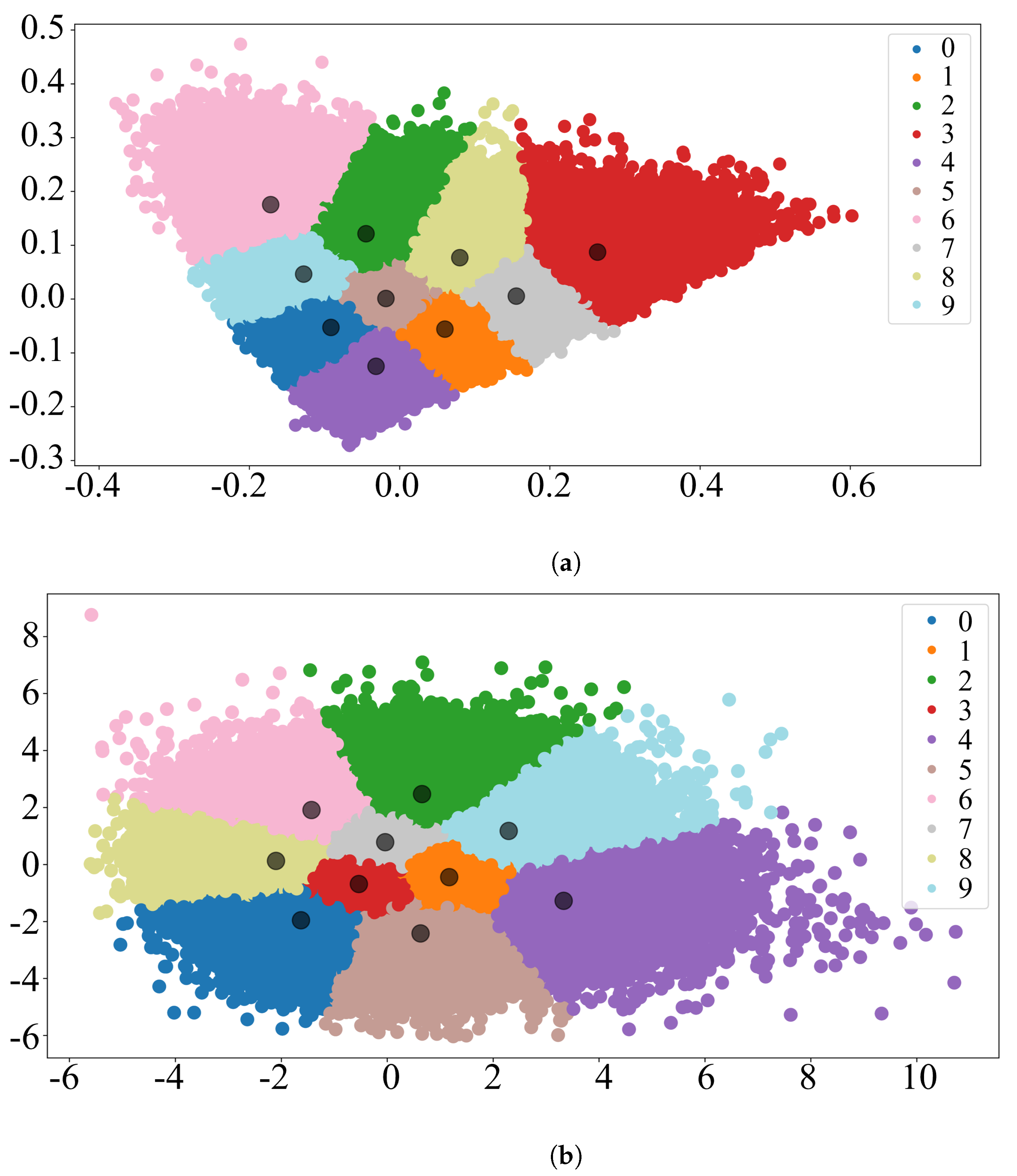


