Dynamics of Classical Solutions of a Two-Stage Structured Population Model with Nonlocal Dispersal

Abstract

We study the dynamics of classical solutions of a two-stage structured population model with nonlocal dispersal in a spatially heterogeneous environment and address the question of the persistence of the species. In particular, we show that the species’ persistence is completely determined by the sign of the principal spectrum point, ${\lambda }_p$, of the linearized system at the trivial solution: the species goes extinct if ${\lambda }_p\le 0$, while it persists uniformly in space if ${\lambda }_p>0$. Sufficient conditions are provided to guarantee the existence, uniqueness, and stability of a positive steady state when the parameters are spatially heterogeneous. Furthermore, when the model parameters are spatially homogeneous, we show that the unique positive equilibrium is globally stable with respect to positive perturbations.

1. Introduction

In this work, we study the dynamics of solutions of the nonlocal system of partial differential equations (PDE)

$$\left\{\begin{array}{cc}{\partial }_t{u}_1={\mu }_1{\int }_{\Omega }\kappa (x,y)(u_1(t,y)-u_1(t,x))dy+r{u}_2-s{u}_1-(a+b{u}_1+\tau c{u}_2)u_1\hfill & x\in \Omega ,t>0,\hfill \\ {\partial }_t{u}_2={\mu }_2{\int }_{\Omega }\kappa (x,y)(u_2(t,y)-u_2(t,x))dy+s{u}_1-(e+f{u}_2+\tau g{u}_1)u_2\hfill & x\in \Omega ,t>0,\hfill \end{array}\right.$$

(1)

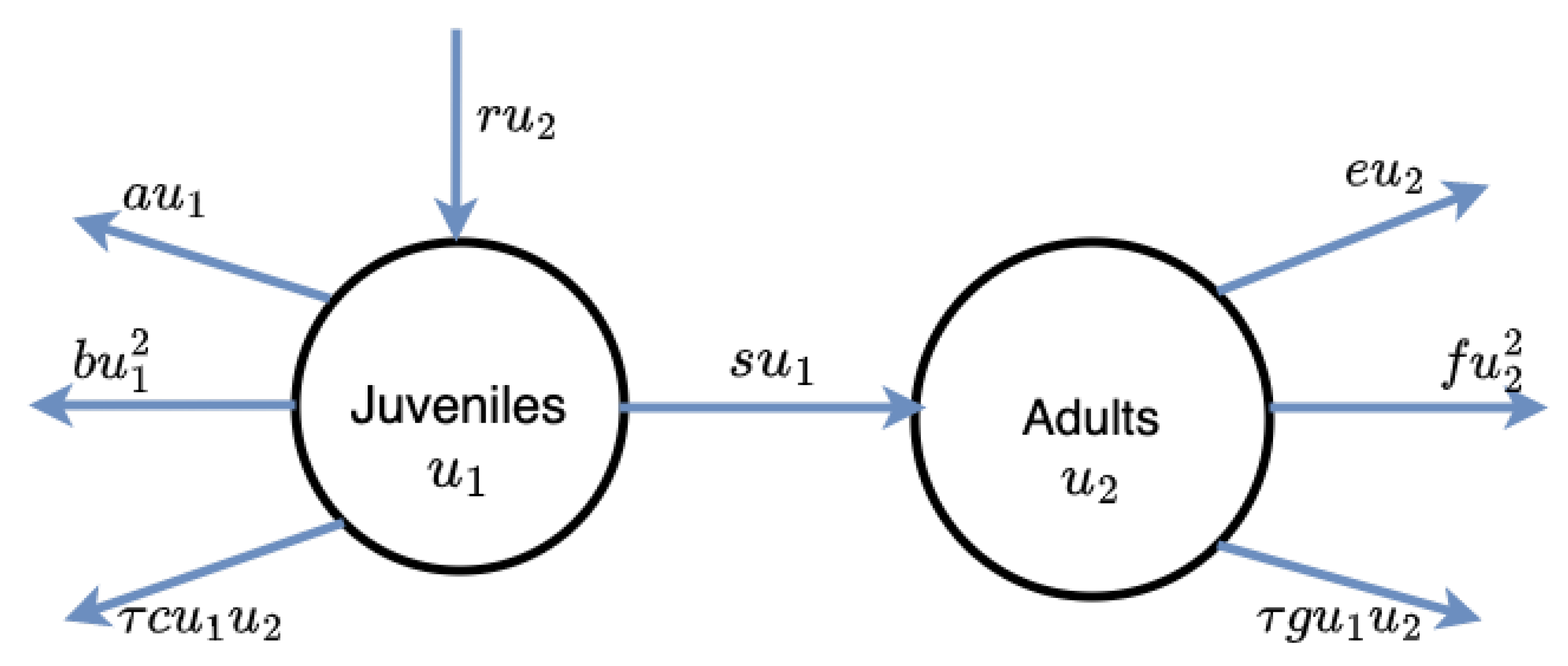
where $\mathbf{u}(t,x)=(u_1(t,x),u_2(t,x))$ represents the density function of a single species structured into two stages (juveniles and adults) and living in a bounded habitat $\Omega \subset {\mathbb{R}}^n$: $u_1(t,x)$ denotes the density function of the juveniles and $u_2(t,x)$ that of the adults who have reached reproductive maturity age. The adults have local reproductive rate $r(x)$ and the juveniles attain reproductive maturity at the rate $s(x)$. The juveniles have local death rate $a(x)$ and self-limitation rate $b(x)$ due to their size in space. The adults have a local death rate $e(x)$ and local self-limitation rate $f(x)$ induced by their size. Due to the interaction between the adults and the juveniles, there may exist an interspecific competition for local resources. Then, we denote by $\tau c(x)$ and $\tau g(x)$ the interspecific local competition rates of the adults and juveniles, respectively. Here, $\tau$ is a non-negative number and measures the strength of the interspecific competition. See Figure 1 below for a schematic illustration of the model. Throughout this work, we shall suppose that the kernel function $\kappa$ is uniformly continuous, positive, and symmetric, i.e., $\kappa (x,y)=\kappa (y,x)>0$ for every $x,y\in \overline{\Omega }$. Furthermore, we suppose that the parameters of system (1) satisfy the following standing hypothesis.

Hypothesis 1.

The functions $a,b,c,e,f,g,r$, and s are Hölder continuous on $\overline{\Omega }$ and non-negative, r and s are non-identically zero, and b and f are strictly positive.

System (1) is the nonlocal dispersal counterpart of the following population system with random (local) dispersal and Neumann boundary conditions

$$\left\{\begin{array}{cc}{\partial }_t{u}_1={\mu }_1\Delta u_1+r{u}_2-s{u}_1-(a+b{u}_1+\tau c{u}_2)u_1\hfill & x\in \Omega ,t>0,\hfill \\ {\partial }_t{u}_2={\mu }_2\Delta u_2+s{u}_1-(e+f{u}_2+\tau g{u}_1)u_2\hfill & x\in \Omega ,t>0,\hfill \\ \nabla u_1·\nu =\nabla u_2·\nu =0\mathrm{on}\partial \Omega ,t>0,\hfill \end{array}\right.$$

(2)

where $\nu$ is the outward unit normal to $\partial \Omega .$ The parameters of system (2) have the same meaning as those of system (1). The models (1) and (2) describe the population dynamics of a dispersing species structured into two-stage subpopulations. The authors in [1,2] studied the model (2) as a problem in optimal control. Most studies on population models typically investigate different species competing for shared resources under the assumption that each species has similar characteristics among its kind. However, it is natural for species to involve individuals at different maturity stages who exhibit varying characteristics which significantly influence their survival or extinction. Consequently, several authors have studied the population dynamics of stage-structured species with a random dispersal mechanism (see for example [1,2,3,4,5,6,7] and the references therein). Typically, their analysis on the dynamics of the system depends on the sign of the principal eigenvalue of the linearization of the system at the zero solution. In particular, it was shown in [3] that when $b=\tau c$ and $f=\tau g$ are positive constants, system (2) has a positive steady state if and only if the principal eigenvalue of its linearization at the zero solution is positive.

For unstructured population models for which species dispersal is modeled by pure diffusion, it is known that slow diffusion is advantageous for species’ survival (see [8,9,10,11] and the references therein). Recently, in [4], the authors examined the influence of diffusion rates on the persistence and extinction of the stage-structured model with random dispersal (2). Their theoretical results indicated that the persistence and extinction of the species depend on the spatial distribution of favorable habitats for the different subpopulations. Essentially, if the regions where adults can reproduce are the same as those where juveniles can mature, typically slow diffusion guarantees persistence, but if those regions are separated, then faster diffusion may be advantageous for the species’ survival.

It is typical to assume that a species’ dispersal is governed by random walking between adjacent spatial locations. Such an assumption give rise to local dispersal models such as (2). However, some organisms can move between non-adjacent spatial locations, exhibiting long-range dispersal. Nonlocal dispersal equations of the form (1) have been employed to model the population dynamics of such species (see [12,13,14,15,16,17]). For the nonlocal dispersal operator ${\int }_{\Omega }\kappa (x,y)(u_i(t,y)-u_i(t,x))dy$ in (1), $\kappa (x,y)$ is a probability density function that gives the probability of jumping from location y to x. Thus, since $u_i(t,x)$ gives the population density at time t and location x, ${\int }_{\Omega }\kappa (x,y)u_i(t,y)dy$ gives the rate at which individuals from other places arrive at location x and $-{\int }_{\Omega }\kappa (x,y)u_i(t,x)dy$ gives the rate at which they leave location x.

Typical examples of such kernel function include the probability density function of the normal distribution

$$\kappa (x,y)=\kappa (x-y)=\frac{1}{\sqrt{{(2\pi )}^n}}{e}^{-\frac{{|x-y|}^2}{2}}x,y\in {\mathbb{R}}^n.$$

In [16], the authors established the relationship between such random dispersal equations such as (2) with Neumann boundary conditions and the nonlocal dispersal Equation (1). Hence, Equation (1) can be said to have a Neumann-type boundary condition. The techniques developed in the current work hold for general kernel functions having singularities at $x=y$. Depending on the strength of the singularity in the later types of kernels at $x=y$, they can be used to approximate solutions of fractional Laplacian operators (see [16,18,19,20,21] and the references therein ).

Our goal in this study is to examine to what extent the results obtained for model (2) extend to (1); hence, we study the dynamics of the model (1). Our analysis is based on the spectral bound of the linearization of the model (1) at the zero solution. Our results show that the principal spectrum point (see Definition 2 below) completely determines the persistence or extinction of the species modeled by (1) in the sense that the species die out if the principal spectrum point is nonpositive, but persist uniformly in time when it is positive (see Theorem 1). When persistence occurs, it is appropriate to examine the existence of a strictly positive steady state for the model and its stability with respect to positive perturbations. Understandably, such a steady state depends on the interaction magnitude $\tau$. In the case of a spatially homogeneous environment, our studies show that for any $\tau \ge 0$, the system (1) has a unique positive steady state which attracts every positive solution (see Theorem 2). It is pertinent to mention that due to the lack of compactness induced by the nonlocal operators, the analysis of nonlocal dispersal systems pose extra challenge than their local dispersal counterparts. Nevertheless, for the spatially heterogeneous environment, we obtained sufficient conditions for the existence, uniqueness and local stability of a positive stationary solution of (1) when $\tau >0$ (see Theorems 3 and 4). Given that the persistence of the species modeled by (1) depends on the sign of the principal spectrum point, we established some criteria on the model parameters for the positivity or otherwise of the principal spectrum point. Thus, Theorem 5 provides sufficient conditions on the parameters for the persistence or extinction of the species.

The rest of the paper is organized as follows. Section 2 contains notations, definitions, and the main results. In Section 3, we provide a brief discussion of our theoretical results on model (1), compare them to some related results on model (2), and highlight some future directions. The proof of our main results are presented in Appendix A, Appendix B and Appendix C.

2. Notations, Definitions and Main Results

2.1. Notations and Definitions

Before stating our main results on the classical solutions of (1), we first introduce a few notations and definitions. Let $X:=C(\overline{\Omega })$ denote the Banach space of uniformly continuous and bounded functions on $\overline{\Omega }$ endowed with the sup-norm; ${\parallel u\parallel }_{\infty }={\displaystyle \underset{x\in \Omega }{sup}}|u(x)|$ for every $u\in X$. Since the density functions are non-negative, we will be interested in the following subsets of X:

$$X^{+}=\{u\in X|u(x)\ge 0,x\in \overline{\Omega }\},$$

and

$$X^{++}=\{u\in X^{+}|\underset{x\in \overline{\Omega }}{inf}u(x)>0\}.$$

We shall use bold-face letters to represent vectors. In particular, we use $\mathbf{u}=(u_1,u_2)$ to denote vectors in ${\mathbb{R}}^2$. For convenience, we also use $\mathbf{u}=(u_1,u_2)$ for elements of $X\times X$. Hence, any vector in ${\mathbb{R}}^2$ can be understood as a constant vector valued function on $\overline{\Omega }$; this would not cause any confusion in the paper. We endow $X\times X$ with the norm

$$\parallel \mathbf{u}\parallel :=max\{\parallel u_1{\parallel }_{\infty },\parallel u_2{\parallel }_{\infty }\}\forall \mathbf{u}=(u_1,u_2)\in X\times X.$$

Hence, $X\times X$ is also a Banach space. Given a function $l\in X$, we set

$$l_{min}:=\underset{x\in \overline{\Omega }}{min}l(x)\mathrm{and}{l}_{max}=\underset{x\in \overline{\Omega }}{max}l(x).$$

We consider the following ordering in $X\times X$:

$$\mathbf{u}\le 1\mathbf{v}\mathrm{if}{v}_i-u_i\in X^{+},i=1,2\mathrm{and}\mathbf{u}<1\mathbf{v}\mathrm{if}{v}_i-u_i\in X^{++},i=1,2.$$

(3)

We adopt the following definition for classical solutions of (1).

Definition 1.

Let $\tau \ge 0$, ${\mathbf{u}}_0=(u_{1,0},u_{2,0})\in X^{+}\times X^{+}$ and $T\in (0,\infty ]$. We say that a function $\mathbf{u}(·,·;\tau ,{\mathbf{u}}_0)\in C([0,T)\times \overline{\Omega })$ is a classical solution of (1) with initial data ${\mathbf{u}}_0$ if it is continuously differentiable with respect to t on $[0,T)$, satisfies (1) in the classical sense, $\mathbf{u}(t,·;\tau ,{\mathbf{u}}_0)\in X^{+}\times X^{+}$ for every $t\in [0,T)$ and

$$\underset{t\to 0^{+}}{lim}\parallel \mathbf{u}(t,·;\tau ,{\mathbf{u}}_0)-{\mathbf{u}}_0\parallel =0.$$

When $T=\infty$, we say that the classical solution $\mathbf{u}(·,·;\tau ,{\mathbf{u}}_0)$ is globally defined in time.

Thanks to the type of nonlinearity in (1), the following result on the existence and uniqueness of classical solutions of system (1) follows from standard arguments from the literature on semigroup theory and positivity of semigroup generated by nonlocal operators [22,23].

Proposition 1.

Let $\tau \ge 0$. Given any initial data ${\mathbf{u}}_0\in X^{+}\times X^{+}$, there is a unique corresponding global and bounded classical solution $\mathbf{u}(t,·;\tau ,{\mathbf{u}}_0)$. Moreover, if ${\mathbf{u}}_0$ is not identically null, then $\mathbf{u}(t,·;\tau ,{\mathbf{u}}_0)\in X^{++}\times X^{++}$ for all $t>0$.

It is clear that the null function $\mathbf{0}\equiv (0,0)$, called the trivial solution, is an equilibrium solution of (1). To study the stability of the trivial solution, the sign of the "principal spectrum point" of the linearization of model (1) at $\mathbf{0}$ will be essential. For convenience, we first recall the following definition.

Definition 2

(Principal spectrum point). Let E be a Banach space and $B:dom(B)\to E$ be a linear map where $dom(B)$ is a linear subspace of E. Let $\sigma (B)$ denote the spectrum of B. The principal spectrum point (PSP) of B, denoted by ${\lambda }_p(B)$, is defined as

$${\lambda }_p(B):=\left\{\begin{array}{cc}sup\{\mathbf{Re}(\lambda ):\lambda \in \sigma (B)\}\hfill & if\sigma (B)\ne \varnothing ,\hfill \\ -\infty \hfill & if\sigma (B)=\varnothing .\hfill \end{array}\right.$$

For our purpose in the current work, the Banach space in Definition 2 will be either $E=X$ or $E=X\times X$, while the linear operator B will always be a bounded linear map on E. Hence, in the current work, $\sigma (B)$ will always be nonempty and bounded, so that the PSP ${\lambda }_p(B)$ is a real number.

Given $h\in X$, consider the bounded linear operators $\mathcal{K},\mathcal{I},h\mathcal{I}:X\to X$

$$\mathcal{K}u(x)={\int }_{\Omega }\kappa (x,y)(u(y)-u(x))dy\forall u\in X,x\in \overline{\Omega },$$

(4)

$$\mathcal{I}u(x)=u(x)\forall u\in X,x\in \overline{\Omega },$$

(5)

and

$$(h\mathcal{I})u(x)=h(x)u(x)\forall u\in X,x\in \overline{\Omega }.$$

(6)

Next, given a bounded linear operator $\mathcal{B}$ on X and a real vector $\mathbf{z}=(z_1,z_2)\in {\mathbb{R}}^2$, we denote by $\mathbf{z}\circ \mathcal{B}$ the bounded linear operator on $X\times X$ given by

$$\mathbf{z}\circ \mathcal{B}\mathbf{u}=\left(\begin{array}{c}{z}_1\mathcal{B}{u}_1\\ z_2\mathcal{B}{u}_2\end{array}\right)\forall \mathbf{u}\in X\times X.$$

(7)

For convenience, set

$$A(x)=\left(\begin{array}{cc}-(a(x)+s(x))& r(x)\\ s(x)& -e(x)\end{array}\right)\forall x\in \overline{\Omega },$$

(8)

and define the bounded linear operator $\mathcal{A}:X\times X\to X\times X$,

$$(\mathcal{A}\mathbf{u})(x)=A(x)\mathbf{u}(x)=\left(\begin{array}{c}r(x)u_2(x)-(a(x)+s(x))u_1(x)\\ s(x)u_1(x)-e(x)u_2(x)\end{array}\right)\forall \mathbf{u}\in X\times X,x\in \overline{\Omega }.$$

(9)

Note that by the Perron-Frobenius theorem, for every $x\in \overline{\Omega }$, the cooperative matrix $A(x)$ has a maximal eigenvalue, which we shall denote by $\Lambda (x)$.

2.2. Main-Results

We state our main results in the current subsection. Our first result is on the global stability of the trivial solution $\mathbf{0}$.

Theorem 1.

Let $\tau \ge 0$ and ${\lambda }_p(\mu \circ \mathcal{K}+\mathcal{A})$ be the PSP of the bounded linear map $\mu \circ \mathcal{K}+\mathcal{A}$. Let $\mathbf{u}(·,·;\tau ,{\mathbf{u}}_0)$ be a classical solution of (1) with a positive initial data ${\mathbf{u}}_0\in X^{+}\times X^{+}\backslash \{\mathbf{0}\}$.

(i)

If ${\lambda }_p(\mu \circ \mathcal{K}+\mathcal{A})<0$, then for every $\xi \in (0,1)$, there is $t_{\xi }>0$, independent of initial data and τ such that

$$\parallel \mathbf{u}(t,·;\tau ,{\mathbf{u}}_0)\parallel \le e^{t\xi {\lambda }_p(\mu \circ \mathcal{K}+\mathcal{A})}\parallel {\mathbf{u}}_0\parallel ,\forall t>t_{\xi }.$$

(10)

(ii)

If ${\lambda }_p(\mu \circ \mathcal{K}+\mathcal{A})=0$, then

$$\underset{t\to \infty }{lim}\underset{\tau \ge 0}{sup}\parallel \mathbf{u}(t,·;\tau ,{\mathbf{u}}_0)\parallel =0.$$

(11)

(iii)

If ${\lambda }_p(\mu \circ \mathcal{K}+\mathcal{A})>0$, then there is ${\eta }_{*}>0$, independent of initial data, such that

$$\underset{t\to \infty }{lim\; sup}\parallel \mathbf{u}(t,·;\tau ,{\mathbf{u}}_0)\parallel \ge {\eta }_{*}.$$

(12)

Furthermore if $r\in X^{++}$ and $s\in X^{++}$, then there is ${\eta }^{*}>0$ which depends on the initial data ${\mathbf{u}}_0$ and τ, such that

$$u_i(t,x;\tau ,{\mathbf{u}}_0)\ge {\eta }^{*},t\ge 1,x\in \Omega ,i=1,2.$$

(13)

It follows from Theorem 1 that the sign of ${\lambda }_p(\mu \circ \mathcal{K}+\mathcal{A})$ determines completely the persistence of the species. Indeed, if ${\lambda }_p(\mu \circ \mathcal{K}+\mathcal{A})\le 0$, then by Theorem 1 (i) and (ii), every classical solution eventually goes extinct in the long run uniformly in space. However, if ${\lambda }_p(\mu \circ \mathcal{K}+\mathcal{A})>0$, then the species persists uniformly in the sense of (13). It is important to note that ${\lambda }_p(\mu \circ \mathcal{K}+\mathcal{A})$ is independent of the non-negative parameter $\tau \ge 0$. Hence, the persistence or extinction of the species is independent of the magnitude of $\tau$.

A natural quest is to understand the long-time behavior of classical solutions of (1) when ${\lambda }_p(\mu \circ \mathcal{K}+\mathcal{A})>0$. In particular, we are interested in whether (1) has a stable steady-state solution which attracts all positive solutions whenever ${\lambda }_p(\mu \circ \mathcal{K}+\mathcal{A})>0$. In this direction, when all the parameters are independent of x, our next result shows that (1) has a unique positive equilibrium point which attracts every classical solution. More specifically, the following result holds.

Theorem 2.

Suppose that ${\lambda }_p(\mu \circ \mathcal{K}+\mathcal{A})>0$ and $a,b,c,e,f,$ r, and s are spatially homogeneous. Then for every $\tau \ge 0$, (1) has a unique constant positive steady-state solution ${\mathbf{u}}^{\tau }$. Moreover, given any positive initial data ${\mathbf{u}}_0$, $\mathbf{u}(t,·;\tau ,{\mathbf{u}}_0)$ converges to ${\mathbf{u}}^{\tau }$ as t tends to infinity in the sense that

$$\underset{t\to \infty }{lim}\parallel \mathbf{u}(t,·;\tau ,{\mathbf{u}}_0)-{\mathbf{u}}^{\tau }\parallel =0.$$

(14)

Thanks to Theorems 1 and 2, the global dynamics of classical solutions of system (1) are well understood when the parameters in the model are spatially homogeneous. However, when these parameters depend on x and ${\lambda }_p(\mu \circ \mathcal{K}+\mathcal{A})>0$, the existence and uniqueness of a positive steady state remain unclear. This is due to the lack of compactness induced by the nonlocal operators used to describe the dispersal modes of the species and the fact that the flow of classical solutions induced by (1) is not monotone when $\tau >0$.

When the parameters depend on x and $\tau =0$, system (1) is cooperative, and some standard methods, based on the theory of monotone dynamical systems from the literature, can be employed to study the global dynamics of the classical solutions (see [24]). Our next result provides some sufficient conditions, which guarantees the existence, uniqueness, and local stability of a positive steady state of system (1) when $\tau >0$. In the next two results, we suppose that the parameter functions depend on the variable x.

Theorem 3.

(i)

Let $\mu >0$ such that ${\lambda }_p(\mu \circ \mathcal{K}+\mathcal{A})>0$. Then there is ${\tau }^{*}\in (0,\infty ]$ such that for every $\tau \in [0,{\tau }^{*})$, (1) has a unique positive steady state solution ${\mathbf{u}}^{\tau }\in X^{++}\times X^{++}$. Moreover, for every $\tau \in [0,{\tau }^{*})$, ${\mathbf{u}}^{\tau }$ is linearly stable.

(ii)

If ${\Lambda }_{min}>0$, then for every $\tau >0$, there is ${\mu }^{\tau }>0$ such that for every diffusion rate $\mu =({\mu }_1,{\mu }_2)$ satisfying $0<{\mu }_i<{\mu }^{\tau }$, (1) has a unique positive steady state solution ${\mathbf{u}}^{\mu ,\tau }\in X^{++}\times X^{++}$. Furthermore, ${\mathbf{u}}^{\mu ,\tau }$ is linearly stable.

For each $\mu$ for which ${\lambda }_p(\mu \circ \mathcal{K}+\mathcal{A})>0$, Theorem 3 (i) shows that system (1) has a unique and linearly stable positive steady state for every $\tau \in [0,{\tau }^{*})$. Note from Theorem 2 that ${\tau }^{*}=\infty$ when the parameters are spatially homogeneous. In general, when the parameters depend on the spatial variable, it is unclear whether ${\tau }^{*}=\infty$. Our next result is concerned with the global stability of the positive steady state given by Theorem 3.

Theorem 4.

Suppose that ${\lambda }_p(\mu \circ \mathcal{K}+\mathcal{A})>0$. The following conclusions hold.

(i)

If $\tau =0$, then the unique strictly positive steady state ${\mathbf{u}}^0$ of (1) is globally stable with respect to positive perturbations in the sense of (14).

(ii)

If $r_{min}>0$ and $s_{min}>0$, then there is ${\tau }^{**}\in (0,{\tau }^{*}]$, where ${\tau }^{*}$ is given by Theorem 3(i)such that for every $\tau \in [0,{\tau }^{**})$ the unique positive steady state ${\mathbf{u}}^{\tau }$ of (1) is globally stable with respect to positive perturbations in the sense of (14).

Next, we examine some sufficient conditions on the spatial heterogeneity of model (1) to determine the sign of ${\lambda }_p(\mu \circ \mathcal{K}+\mathcal{A})$ for any diffusion rate $\mu =({\mu }_1,{\mu }_2)$. First, note that ${\lambda }_p(\mu \circ \mathcal{K}+\mathcal{A})$ is independent of the diffusion rate $\mu$ when all the parameters are spatially homogeneous. In this case, ${\lambda }_p(\mu \circ \mathcal{K}+\mathcal{A})$ equals the maximal eigenvalue of the cooperative matrix A. In general, when the parameters depend on the space variable x, ${\lambda }_p(\mu \circ \mathcal{K}+\mathcal{A})$ may not be an eigenvalue (see [25,26] for examples). Moreover, in such a case, there is no explicit variational characterization formula for ${\lambda }_p(\mu \circ \mathcal{K}+\mathcal{A})$. From the application viewpoint, it is of particular importance to find sufficient conditions to determine the sign of ${\lambda }_p(\mu \circ \mathcal{K}+\mathcal{A})$. Inspired by the results in [4], we have the following result.

Theorem 5.

Suppose that ${(a+s)}_{min}>0$ and $e_{min}>0$.

(i)

If either ${\left(\frac{s}{e}\right)}_{max}{\left(\frac{r}{s+a}\right)}_{max}<1$ or ${\left(\frac{4{(r+s)}^2}{e(a+s)}\right)}_{max}<1$, then ${\lambda }_p(\mu \circ \mathcal{K}+\mathcal{A})<0$ for any diffusion rate $\mu =({\mu }_1,{\mu }_2)$.

(ii)

If either ${\left(\frac{s}{e}\right)}_{min}{\left(\frac{r}{s+a}\right)}_{min}>1$ or ${\int }_{\Omega }\sqrt{rs}>\frac{1}{2}{\int }_{\Omega }(a+s+e)$, then ${\lambda }_p(\mu \circ \mathcal{K}+\mathcal{A})>0$ for any diffusion rate $\mu =({\mu }_1,{\mu }_2)$.

Theorem 5 provides sufficient hypotheses on the parameters which guarantee that the sign of ${\lambda }_p(\mu \circ \mathcal{K}+\mathcal{A})$ is independent of the diffusion rate $\mu$ of the species. Note that, when the parameters are spatially homogeneous, $\Lambda :=\Lambda (x)$ is independent of $\mu$ and $\Lambda >0$ if $sr>(a+s)e$, $\Lambda =0$ if $rs=(a+s)e$, and $\Lambda <0$ if $rs<(a+s)$. Hence, the first assumption in Theorem 5 (i) and (ii) are consistent with that of the ODE model. Next, observe that $\frac{s}{e}$ (resp. $\frac{r}{s+a}$) is the ratio of the growth rate to the self-limitation rate of the adults (resp. juveniles). Hence, on one hand, Theorem 5 (i) indicates that if the product of the maximum of these ratios is smaller than one, then species cannot survive and will go extinct in the long run irrespective of the diffusion rate. On the other hand, if the product of the minimum of these ratios is greater than one, Theorem 5 (ii) indicates that the species will always persist uniformly in space for any diffusion rate.

3. Conclusions and Future Directions

In this study, we examined the dynamics of classical solutions of a population adopting a long-range dispersal migration and structured in two stages, juveniles and adults. In particular, we addressed the question of the persistence of the species. In this direction, Theorem 1 indicates that the sign of the principal spectrum point ${\lambda }_p$ of the linearization of system (1) at the trivial solution completely determines the species’ persistence or extinction. More precisely, if ${\lambda }_p\le 0$, the species eventually goes extinct uniformly in space while it persists uniformly in space if ${\lambda }_p>0$. This result agrees with the dynamics of classical solutions of model (2) where a random local dispersal is used to describe the evolution of the species. Indeed, Cantrell, Cosner, and Martinez (Lemma 2 in [4]) showed that if the principal eigenvalue, ${\lambda }_{eig,p}$, of the linearization of system (2) at the trivial solution is positive, then the species persists uniformly in space while it goes extinct otherwise. Note that the analyses of system (2) rely largely on the compactness of its solution operator; however, the semiflow generated by classical solutions of (1) is not compact. Consequently, ${\lambda }_p$ might not be an eigenvalue. This lack of compactness of the semiflow generated by classical solutions of system (1) induces some difficulties, and several techniques developed for system (2) cannot be applied to system (1).

When ${\lambda }_p>0$ and the environment is homogeneous, Theorem 2 shows that the species eventually stabilize in the long run at the unique stationary equilibrium solution. Our proof of this result relies on constructing a delicate Lyapunov function (see Lemma A3). This Lyapunov function is concave and can also be used to obtain the global stability of classical solutions of system (2) and the corresponding kinetic model. It is important to note that Bouguima and Mehlia (Theorem 2.1 in [27]) used the Poincaré–Bendixon theory to conclude the uniqueness and global stability of the unique stationary equilibrium for the kinetic model. However, this method is only suitable for the ODE model.

When the environment is heterogeneous, and ${\lambda }_p>0$ under suitable smallest assumption on the interspecific competitions terms between the juveniles and the adults, Theorems 3 and 4 guaranteed the existence and stability of a positive steady state solution of system (1). It would be of great interest to know whether (1) always has a unique and globally stable positive steady state solution whenever ${\lambda }_p>0$. This question also remains open for system (2). In this direction, for system (2) and when ${\lambda }_{eig,p}>0$, it is important to note that Brown and Zhang (Theorem 3.2 in [3]) established the existence of at least one positive steady state, Bouguima and Mehlia (Propositision 6.1 in [27]) obtained a sufficient condition of the initial data which guarantee the global stability of the unique positive steady state solution, and Cantrell, Cosner, and Martinez (Lemma 3 in [4]) conclude the global stability of the positive steady solution if $\tau$ is sufficiently small.

There are several important prospects to consider in future studies on the dynamics of solutions of (1).

(i)

Effect of dispersal rates on ${\lambda }_p.$ The necessary and sufficient condition for persistence is the positivity of ${\lambda }_p$. Unlike the case of unstructured single species and local reaction diffusion equation, there is no explicit formula for ${\lambda }_p$. This makes the study of ${\lambda }_p$ with respect to the diffusion rates difficult. However, in several instances, juveniles do not move or move very slowly whereas adults have a high movement rate. This is the case for some species of birds. Hence, it is of great biological interest to study the asymptotic behavior of ${\lambda }_p$ when one of the diffusion rates is small while the other is large.

(ii)

Global stability of positive steady states. Understanding the long-time behavior of classical solutions of model (1) is essential since it helps to provide some accurate prediction on the future of the species. In the current work, we completely settled this question in the case of a homogeneous environment or the smallest assumption on $\tau$. Further efforts are needed for the case of arbitrary $\tau >0$.

(iii)

Asymptotic profile of positive steady states with respect to diffusion rates. When species persist and eventually stabilize, from an ecological viewpoint, it is important to know the spatial distribution of the species. This would be determined by the influence of the diffusion rates on the steady states. In this direction, we hope that future works would explore the dependence of positive steady-state solutions of system (1) on the diffusion rates.

(iv)

Effect of temporal heterogeneity on the dynamics of (1). An important fact not considered in our study is the effect of temporal heterogeneity on the dynamics of solutions of model (1). It would be of important biological interest to study the dynamics of solutions of (1) in time-periodic environments.

References

- Arino, O.; Montero, J.A. Optimal control of a nonlinear elliptic population system. Proc. Edinb. Math. Soc. 2000, 116, 225–241. [Google Scholar] [CrossRef]
- Canada, A.; Magal, P.; Montero, J.A. Optimal control of harvesting in a nonlinear elliptic system arising from population dynamics. J. Math. Anal. Appl. 2001, 254, 571–586. [Google Scholar] [CrossRef]
- Brown, K.J.; Zhang, Y. On a system of reaction-diffusion equations describing a population with two age groups. J. Math. Anal. Appl. 1980, 282, 444–452. [Google Scholar] [CrossRef]
- Cantrell, R.S.; Cosner, C.; Martinez, S. Persistence for a two-stage reaction-diffusion system. Mathematics 2020, 8, 396. [Google Scholar] [CrossRef]
- Cantrell, R.S.; Cosner, C.; Yu, X. Population with individual variation in dispersal in heterogeneous environments: Dynamics and competition with simply diffusing populations. Sci. Chi. Math. 2020, 63, 441–464. [Google Scholar] [CrossRef]
- Cantrell, R.S.; Cosner, C.; Yu, X. Dynamics of populations with individual variation in dispersal in bounded domains. J. Biol. Dyn. 2018, 12, 288–317. [Google Scholar] [CrossRef]
- Henaoui, O. An elliptic system modeling two subpopulations. Nonlinear Anal. Real World Appl. 2012, 13, 2447–2458. [Google Scholar] [CrossRef]
- Cosner, C.; Lazer, A.C. Stable coexistence states in the Volterra-Lotka competition model with diffusion. SIAM J. Appl. Math. 1984, 44, 1112–1132. [Google Scholar] [CrossRef]
- Dockery, J.; Hutson, V.; Mischaikow, K.; Pernarowski, M. The evolution of slow dispersal rates: A reaction-diffusion model. J. Math. Biol. 1998, 37, 61–83. [Google Scholar] [CrossRef]
- Hastings, A. Can spatial variation alone lead to selection for dispersal? Theor. Popul. Biol. 1983, 24, 244–251. [Google Scholar] [CrossRef]
- Hetzer, G.; Nguyen, T.; Shen, W. Coexistence and extinction in the volterra-Lotka competition model with nonlocal dispersal. Commun. Pure Appl. Anal. 2012, 11, 1699–1722. [Google Scholar] [CrossRef]
- Bao, X.; Shen, W. Criteria for the existence of principal eigenvalues of time periodic cooperative linear systems with nonlocal dispersal. Proc. Am. Math. Soc. 2017, 145, 2881–2894. [Google Scholar] [CrossRef]
- Rawal, N.; Shen, W. Criteria for the existence and lower bounds of principal eigenvalues of time periodic nonlocal dispersal operators and applications. J. Dynam. Differ. Equ. 2012, 24, 927–954. [Google Scholar] [CrossRef]
- Onyido, M.A.; Shen, W. Nonlocal dispersal equations with almost periodic dependence. I. Principal spectral theory. J. Differ. Equ. 2021, 295, 1–38. [Google Scholar] [CrossRef]
- Shen, W.; Xie, X. On principal spectrum points/principal eigenvalues of nonlocal dispersal operators and applications. Disc. Cont. Dyn. Syst. 2015, 35, 1665–1696. [Google Scholar] [CrossRef]
- Shen, W.; Xie, X. Approximations of random dispersal operators/equations by nonlocal dispersal operators/equations. J. Differ. Equ. 2015, 259, 7375–7405. [Google Scholar] [CrossRef]
- Shen, W.; Zhang, A. Traveling wave solutions of Spatially periodic Nonlocal monstable equations. Commun. Appl. Nonlinear Anal. 2012, 19, 73–101. [Google Scholar]
- Antil, H.; Dondl, P.; Striet, L. Analysis and Approximation of Nonlocal Diffusion Problems with Volume Constraints. SIAM Rev. 2012, 54, 667–696. [Google Scholar]
- Cortazar, C.; Elgueta, M.; Rossi, J.D.; Wolanski, N. How to approximate the heat equation with Neumann boundary conditions by nonlocal diffusion problems. Arch. Ration. Mech. Anal. 2007, 187, 137–156. [Google Scholar] [CrossRef]
- D’Elia, M.; Gunzburger, M. The fractional Laplacian operator on bounded domains as a special case of the nonlocal diffusion operator. Comput. Math. Appl. 2013, 66, 1245–1260. [Google Scholar] [CrossRef]
- Duo, S.; Wang, H.; Zhang, Y. A comparative study on nonlocal diffusion operators related to the fractional Laplacian. Discret. Contin. Dyn. Syst. B 2019, 24, 231–256. [Google Scholar] [CrossRef]
- Henry, D. Geometric Theory of Semilinear Parabolic Equations; Lecture Notes in Mathematics (LNM); Springer: Berlin/Heidelberg, Germany, 2006; Volume 840. [Google Scholar]
- Pazy, A.L. Semigroups of Linear Operators and Applications to Partial Differential Equations; Springer: New York, NY, USA, 1983. [Google Scholar]
- Hess, P. Periodic-Parabolic Boundary Value Problems and Positivity; Pitman Research Notes in Mathematics 247; Longman Scientific & Technical: Harlow, UK, 1991. [Google Scholar]
- Coville, J. On a simple criterion for the existence of a principal eigenfunction of some nonlocal operators. J. Differ. Equ. 2010, 249, 2921–2953. [Google Scholar] [CrossRef]
- Shen, W.; Zhang, A. Spreading speeds for monostable equations with nonlocal dispersal in space periodic habitats. J. Differ. Equ. 2010, 249, 747–795. [Google Scholar] [CrossRef]
- Bouguima1, S.M.; Mehlia, F.Z. Asymptotic behavior of an age-structured population with diffusion. J. Appl. Anal. Comp. 2012, 2, 351–362. [Google Scholar]
- Engel, K.-J.; Nagel, R. One-Parameter Semigroups for Linear Evolution Equations; Springer: New York, NY, USA, 2000. [Google Scholar]
- Kumagai, S. An implicit function theorem: Comment. J. Opt. Theory Appl. 1980, 31, 285–288. [Google Scholar] [CrossRef]
- Magal, P.; Zhao, X.Q. Global attractors and steady states for uniformly persistent dynamical systems. SIAM J. Math. Anal. 2005, 37, 251–275. [Google Scholar] [CrossRef]
- Smith, H.L.; Thieme, H.R. Dynamical Systems and Population Persistence; American Mathematical Society: Providence, RI, USA, 2011; Volume 118. [Google Scholar]
Figure 1.
Illustrative diagram of the dynamics of a population structured in two stages, where is the density of the juveniles and is the density of the adults.
Disclaimer/Publisher’s Note: The statements, opinions and data contained in all publications are solely those of the individual author(s) and contributor(s) and not of MDPI and/or the editor(s). MDPI and/or the editor(s) disclaim responsibility for any injury to people or property resulting from any ideas, methods, instructions or products referred to in the content. |
© 2023 by the authors. Licensee MDPI, Basel, Switzerland. This article is an open access article distributed under the terms and conditions of the Creative Commons Attribution (CC BY) license (https://creativecommons.org/licenses/by/4.0/).
Share and Cite
MDPI and ACS Style
Onyido, M.A.; Salako, R.B.; Uba, M.O.; Udeani, C.I. Dynamics of Classical Solutions of a Two-Stage Structured Population Model with Nonlocal Dispersal. Mathematics 2023, 11, 925. https://doi.org/10.3390/math11040925
AMA Style
Onyido MA, Salako RB, Uba MO, Udeani CI. Dynamics of Classical Solutions of a Two-Stage Structured Population Model with Nonlocal Dispersal. Mathematics. 2023; 11(4):925. https://doi.org/10.3390/math11040925
Chicago/Turabian StyleOnyido, Maria A., Rachidi B. Salako, Markjoe O. Uba, and Cyril I. Udeani. 2023. "Dynamics of Classical Solutions of a Two-Stage Structured Population Model with Nonlocal Dispersal" Mathematics 11, no. 4: 925. https://doi.org/10.3390/math11040925
Note that from the first issue of 2016, this journal uses article numbers instead of page numbers. See further details here.