
Multidimensional Diffusion-Wave-Type Solutions to the Second-Order Evolutionary Equation


Matrosov Institute for System Dynamics and Control Theory of Siberian Branch of Russian Academy of Sciences, Irkutsk 664033, Russia
*
Author to whom correspondence should be addressed.
Mathematics 2024, 12(2), 354; https://doi.org/10.3390/math12020354
Submission received: 8 December 2023
/
Revised: 15 January 2024
/
Accepted: 19 January 2024
/
Published: 22 January 2024
(This article belongs to the Section Difference and Differential Equations)
Abstract
:The paper concerns a nonlinear second-order parabolic evolution equation, one of the well-known objects of mathematical physics, which describes the processes of high-temperature thermal conductivity, nonlinear diffusion, filtration of liquid in a porous medium and some other processes in continuum mechanics. A particular case of it is the well-known porous medium equation. Unlike previous studies, we consider the case of several spatial variables. We construct and study solutions that describe disturbances propagating over a zero background with a finite speed, usually called ‘diffusion-wave-type solutions’. Such effects are atypical for parabolic equations and appear since the equation degenerates on manifolds where the desired function vanishes. The paper pays special attention to exact solutions of the required type, which can be expressed as either explicit or implicit formulas, as well as a reduction of the partial differential equation to an ordinary differential equation that cannot be integrated in quadratures. In this connection, Cauchy problems for second-order ordinary differential equations arise, inheriting the singularities of the original formulation. We prove the existence of continuously differentiable solutions for them. A new example, an analog of the classic example by S.V. Kovalevskaya for the considered case, is constructed. We also proved a new existence and uniqueness theorem of heat-wave-type solutions in the class of piece-wise analytic functions, generalizing previous ones. During the proof, we transit to the hodograph plane, which allows us to overcome the analytical difficulties.
1. Introduction
Let us consider the second-order nonlinear evolutionary equation
where t is time; is Laplacian in spatial variables ; is an unknown function. The given functions are assumed to be sufficiently smooth. If , Equation (1) is parabolic [1].
The most known version of Equation (1) is the porous medium equation [2] also called ‘nonlinear heat equation’ [3]. It corresponds to the case , . Meanwhile, there are other versions [4]. Furthermore, some scientists often deal with such a form of Equation (1), which incorporates terms with the first derivatives of spatial variables—convective terms. This type of equation is called a ‘diffusion–convection equation’ [5].
These equations and systems have been studied for over a century [6] and continue to be crucial and urgent problems in the modern theory of partial differential equations [7] and mathematical physics [8]. Apparently, the reason lies both in interesting mathematical properties and in connection with important physical [3], mechanical [9], and biological [10] applications.
It was the famous French mathematician and physicist J.V. Boussinesque who first obtained the porous medium equation when studying groundwater filtration [6]. This equation is derived from the physical Darcy’s law and Fourier’s law of heat conduction when the diffusion coefficient (thermal conductivity coefficient) depends on density (temperature). It is often used as a simplified mathematical model in the theory of flame propagation theory and the stellar theory [11], as well as to describe an ideal gas filtration in porous media [12]. One can find a more detailed review on applications of nonlinear parabolic equations in monographs [2,5].
Nonlinear parabolic equations and systems with degeneracy are particularly interesting for modern mathematical modeling [13]. For example, it takes place in Equation (1) if . The porous medium equation also has a similar property if . It appears impossible to describe the processes of high-temperature thermal conductivity and filtration of liquids and gases in porous media, where disturbances propagate over a stationary background with a finite velocity, using traditional linear parabolic models. An alternative approach is to use hyperbolic equations [14], but they may not provide required accuracy in modeling [15].
Another way is to apply nonlinear parabolic equations having solutions with the required properties. As far as we know, Ya.B. Zeldovich [11] and G.Ya. Barenblatt [12] are the first who consider such solutions in connection with high-temperature processes in plasma physics and filtration of liquids and gases in porous media, respectively. Note that here we refer not to original articles published in Russian and inaccessible to most readers but to the translated monographs by the same authors.
Later, the term heat [3] (diffusion or filtration [16]) wave, depending on the physical interpretation of the problem, is introduced. Further, we will use the term ’heat wave’ since the equation considered does not include the convective component. A heat wave is defined as a solution to a nonlinear parabolic equation that consists of two parts: positive and zero, joined along a certain surface (line), which is called the ‘wave front’ or ‘zero front’.
So, we are interested in solutions to the generalized porous medium equation with a zero front. They must satisfy both Equation (1) and the condition
where the manifold (zero front) can be given, leading to the problem of constructing a heat wave with a prescribed zero front, or we can determine it via additional conditions. At the zero front, the trivial and nontrivial solutions are continuously joined, and the derivatives, generally speaking, have a discontinuity. Figure 1 shows a geometric illustration of a heat-wave-type solution. The appearance of solutions with nonlinear properties in parabolic equations is seemingly caused by degeneracy at the wave front, leading to so-called ‘locally hyperbolic’ properties.
Since the last quarter of the 20th century, the scientific school of A.F. Sidorov has studied heat-wave-type solutions [16]. A crucial result of these studies is the use of the characteristic series method [8], originally proposed as a tool for studying hyperbolic equations and systems, to solve the problem of heat wave initiation [17,18]. In this case, the coefficients of the series are calculated recursively. The paper [19] concerns methods for constructing exact solutions of the nonlinear heat equation.
The most significant problem for nonlinear parabolic equations and systems is the search for exact solutions [20] with given properties. Much attention is paid to its study at the scientific school of A.A. Samarskii [3]. Thus, N.A. Kudryashov and his disciples study evolutionary equations applied for describing heat conduction processes [21], as well as in the biological Fisher model [22], and the “predator-prey” model [23]. In this regard, a reduction to ordinary differential equations (ODEs) of the Lienard type is often used [24].
Papers [25,26,27,28,29] consider the Cauchy problems for quasilinear parabolic equations. Here, the authors focus on proving the existence of solutions and studying their properties (asymptotic stability, blow-up, localization, etc.).
In [30,31], the authors deal with evolutionary quasilinear parabolic equations with singularities and study various initial-boundary value problems. They prove the existence and uniqueness theorems for weak solutions and investigate blow-up and localization effects in various function spaces.
One of the most prominent specialists in parabolic PDEs is the Spanish mathematician J.L. Vazquez. His research considers the Cauchy problem for quasilinear degenerate parabolic equations, such as the equation with the p-Laplacian operator [32], the fast diffusion equation [33], as well as the porous medium equation [34]. The power-law nature of nonlinearity and the appearance of degeneracy unite all of them. Near the points of degeneracy, as a rule, they observe a finite velocity of propagation of perturbations. The research focuses on abstract functional spaces, proving the existence of a solution and examining asymptotic behavior and blow-up [35], etc. But as a rule, it neither presents explicit formulas of the solution nor constructs solutions as series. Note that, recently, J.L. Vasquez has concentrated on equations with fractional derivatives.
One can find a detailed review of studies of the porous medium equation and its generalizations up to 2007 in the fundamental monograph [2]. Also, our previous articles [36,37] give detailed bibliographic reviews.
We have repeatedly examined zero-front solutions in the context of constructing exact solutions [36,38,39], proving the existence and uniqueness theorems for initial boundary problems that initiate a heat wave [36,38,39], and developing numerical algorithms [37,40]. Moreover, the article [38] provides the immediate background for this study in terms of problem formulation, while the research methods draw from [36,39] to address a higher-dimensional problem.
In this article, we apply more advanced research methods to the previously considered problem, which allows us to obtain new scientific results. In particular, we determine new classes of exact solutions to Equation (1) and either represent them in explicit form or reduce to the integration of ODEs having singularities in the multiplier of the higher derivative. For the ODEs, the existence and uniqueness theorems for classical (smooth) solutions are proven. We also prove a theorem for the existence of analytical solutions to the boundary problem for Equation (1). Unlike [36,38,39], we perform the hodograph transformation in order to overcome analytical difficulties. A new example is constructed, which is an analog of the classic example by S.V. Kovalevskaya [41] and generalizes the earlier result [36].
2. Formulation
Provided that the function is sufficiently smooth and monotonous, it is possible to transform Equation (1) to the following form applying the substitution
Here, , , , in other words, is the inverse function to .
In the presence of spatial symmetries, Equation (3) can be written as
Here, is a new spatial variable, . The most natural cases are (plane symmetry), (cylindrical symmetry), and (spherical symmetry).
A relatively common assumption in the literature is that and are power functions. Then, , , where , are constants, and Equation (4) arrives to the form
The purpose of our study is to obtain solutions to Equation (5), whose construction, as a rule, is reduced to the integration of ordinary differential equations.
The principal (but not the only) interest for us is those solutions that satisfy the condition
since they can be considered as a component of a heat wave.
Obviously, problems (5) and (6) have a trivial solution , but there may be non-trivial ones. The reason for the uniqueness breaking is that Equation (5) degenerates at since the factor of the second (higher) derivative vanishes.
The line , on which the unknown function vanishes, is a zero front.
Looking ahead, we note that solutions with a zero front (if exist) arise as a special case of constructions of a more general type.
3. Heat-Wave-Type Solutions
In this section, we construct exact solutions to (5) and then select those that satisfy condition (6), using various approaches. Speaking about an exact solution, we mean not only explicit or implicit formulas but also the reduction of a partial differential equation to an ordinary differential one, which may not be integrated in quadratures. Of course, not all of the numerous known techniques for constructing exact solutions to equations of mathematical physics [20] are effective in this case, but the range of methods we use is quite wide. Let us look at them successively.
3.1. Polynomial in Powers of
Let us seek a solution to Equation (5) as the following polynomial:
We do not specify the value of yet. Let us substitute (7) into (5) and equate the coefficients at the same powers of .
Analyzing these equalities, we obtain that they can be consistent only if or . Moreover, , and are determined from the ODE system
The initial conditions for system (8) can be set arbitrarily (i.e., there is arbitrariness in two constants). The second equation contains only one unknown function and allows separation of variables.
Let us consider two possible cases
1. If , then , and the second equation of (8) has the following solution:
where is an arbitrary constant.
Note, if , then .
Substituting obtained into the first equation of (8), we obtain another equation with separable variables, which has the solution
where is an arbitrary constant.
Thus, we have the following solution to Equation (5):
Next, let us distinguish such partial solutions (9) that satisfy condition (6) with an unknown zero front . To carry this out, rewrite (9) as
where , and then
One can see that for , the zero front moves away from the origin with exponential speed, and for all admissible .
If , then the zero front moves to the origin, but cannot reach the point , to which it asymptotically approaches. The solution is bounded in t for all admissible .
The most interesting picture is at , when the zero front asymptotically approaches the point , at which Equation (5) has a singularity.
2. When (i.e., no need to choose ), system (8) has a completely different solution
Since , the zero front moves rather slowly. Nevertheless, and is also bounded in t for all admissible .
3.2. Series in Powers of t
An attempt to construct a solution to Equation (5) as a polynomial in powers of t leads to an inconsistent system of equations. So, let us consider the Taylor series
If the initial condition is given as
where is a sufficiently smooth function, the coefficients of the series can be uniquely determined by using the following recurrence formulas:
To calculate , we differentiate the source function as a composite function. The right-hand side of (13) includes only for , which ensures that is uniquely determined if .
The issue of convergence of series (11) requires a separate discussion. The example by S.V. Kovalevskaya for the linear heat equation, known since the 19th century, shows that the solution to the initial problem, which has the form of a power series, can be constructed, but the series is divergent. Similar examples can be given in the nonlinear case.
Previously, we have considered problem (5), (12) for , , and and figured out that series (13) ends if , converges for , and diverges if [36].
Let us now consider the case , , .
1. First, let . Then, in the formula (13) additional non-negative terms appear, which obviously cannot turn divergent series into convergent ones. Thus, series (13) when is divergent, as well as for .
2. Next, let . By induction of k, it can be shown that
which leads to
This solution is a particular case of (10) when . In turn, for we have previously obtained a solution (see (22) from [36]).
3. Finally, let , i.e., . We sequentially calculate the coefficients .
Thus, for and the series does not end (unlike for ). The next coefficient is
By induction of k, it can be shown that
This means that the solution to Equation (5) in this case admits the following form
3.3. Series in Powers of
Let us substitute (14) into (5). Expressing the derivatives and collecting the like terms, we obtain the following problem for the ODE:
The initial condition follows from (12).
The solution to problem (15) is constructed as a series in powers of :
From the initial condition, we have that . Next, from the equation and the initial condition (15), we have that
We determine the rest coefficients by sequentially differentiating Equation (15) and setting . As a result, we have that
One can see that at each step the coefficients found earlier appear on the right side. Moreover, despite the fact that only one initial condition is specified for the second-order equation, the coefficients are determined uniquely. Note that the resulting formulas correspond (up to substitution) to .
Assume the coefficients of the series (16) up to have been found. In order to find , we differentiate Equation (15) k times and set :
where , and the next values are calculated using the formula
Thus, the formal solution to problem (15) in the form of the Maclaurin series at the point is uniquely determined.
The question of the convergence of the constructed series does not generally have a definite answer.
At , as already noted, the series ends and the solution has the form of a linear polynomial. On the other side, let , . Then, .
Let us consider equality (17). The factor multiplying has the following lower estimate
since .
The factor multiplying is positive for .
Finally, in , the factor in square brackets can be represented as
since . Hence, . Moreover, if , then . Therefore,
According to d’Alembert’s criterion, and taking into account (18), the radius of convergence of the power series (16) is determined as
Thus, the series converges only at the point .
The above is justified by the following example.
Example 1.
The problem
has a unique solution in the form of a series in powers of ρ which, for , , diverges everywhere except the point .
Example 1 is an analog of the classic example by S.V. Kovalevskaya and complements the previously proven statement for the plane-symmetric case [36].
Remark 1.
Problem (18) for has a similar property, but the proof requires more subtle and cumbersome estimates.
If we consider for Equation (15) the Cauchy conditions , then, according to the classical existence and uniqueness theorems for ODEs, the problem is uniquely solvable in the class of twice continuously differentiable functions. However, there is a case that does not obey the known theorems, but also leads to the classical solution. Consider the condition . If , without losing the generality, we can set , i.e., deal with the problem
Theorem 1.
Problem (20) has the following classical (twice continuously differentiable) solutions:
- 1.
- If , there is a trivial solution .
- 2.
- If , there is a non-trivial solution having the Taylor series form.
The problem has no other continuously differentiable solutions.
Proof.
The justification for the first part of the theorem is obvious. Let us prove that the second is also true. We construct a solution as the series
From the initial condition, we obtain . Substituting into Equation (20), we obtain . Therefore, either and then we arrive at case 1 since or . For all other values of , the Cauchy problem turns out to be inconsistent, which implies the absence of a classical solution.
Let . Due to determining , we differentiate Equation (20) with respect to and set . Taking into account the previously found derivatives, we find that
Collecting the like terms and expressing , we have that
Continuing to sequentially differentiate Equation (20) and setting , we obtain
where is a polynomial in variables , the explicit form of which is not given here because of the bulkiness. Thus, if derivatives up to order k inclusive are known, the derivative of order is uniquely determined by Formula (22). So, a formal solution in the form of a series has been found.
The convergence of series (21) is proved by constructing a majorant problem of Kovalevskaya type. The construction procedure is also not given because it is cumbersome, since it requires a deep analysis of . □
4. Separation of Variables
Let us now perform in Equation (5) separation of variables according to the following general formula
In fact, we could not use the logarithm, but the chosen method of specifying z allows us to vastly simplify the final form of the equation for v. Similar, though less general, substitutions were applied earlier [36,38].
Substitute the obtained formulas into Equation (5). Collecting the like terms and multiplying by bring us to the equation
which becomes ODE if the following conditions hold:
From the above, we immediately obtain that . Without losing the generality, we can assume . At the same time, it is again necessary to require that either or . Let us consider both cases.
1. Let . Then, , , and the ODE for has the form
Along with it, can be arbitrary, including zero.
2. Let , . Then, , and . Here, , is a real number. In this case, the ODE for turns out to be rather similar:
One can see that only the last terms on the left side differ, more in form than in essence. Equations (24) and (25) can be written jointly as
where can be either or (in the latter case ).
Theorem 2.
Equation (26) in case of it has the following classical (twice continuously differentiable) solutions:
- 1.
- If , there is a trivial solution .
- 2.
- If , there is a non-trivial solution in the Maclaurin series form.
The problem has no other continuously differentiable solutions.
Theorem 2 is proven in the same way as Theorem 1.
5. Qualitative Analysis
Theorem 2 is local and does not allow us to explore global properties of solutions to Equation (26). In order to solve this problem, we perform an analysis of solutions using one of the classical methods of the qualitative theory of differential equations [42]. It helps to study the properties of solution (27) outside a small neighborhood of .
5.1. Analysis of Singular Points
Let us perform some auxiliary transformations. First, we carry out a linear substitution of the independent variable .
Then, (26) takes the form
Here, , . Here, and further, we omit the sign to simplify notation.
Second, since (28) is autonomous, we can lower its order by moving to the phase plane. We consider to be a new unknown function, and v to be an independent variable. Then, (28) becomes
to which the following dynamic system corresponds to
where .
Let us now investigate the equilibrium states (singular points) of system (30). There are three such points: , and . If , then the second and third points coincide.
Let us introduce the following notation:
Let us figure out the type of each singular point.
1. Consider the point . Since , it is a simple equilibrium point; gives the roots of the characteristic equation and . Whereas , , and , the point is the topological saddle.
2. Consider the point . Since , this is a compound equilibrium point. Here, ; therefore, (29) can be written as:
where . Two options are possible and .
2.1. Let . We construct the solution to the equation
as a series in powers of v, which we substitute into . As a result, we obtain
Since the lowest power of v in the expansion equals two, the point is a saddle-node with one nodal and two saddle sectors. The nodal sector is stable because . Moreover, if , then the trajectories of the nodal sector approach when on the left of the axis. If , the trajectories of the nodal sector approach when on the right of the axis.
2.2. Let , then we have following expansions:
Since the lowest power of v in the expansion equals three (odd) and , hence the point is a stable compound node.
5.2. Phase Portrait
Construction and study of a complete phase portrait of dynamic system (30) is a separate and complex issue. In the special case when , it is considered in [37]. Here, we consider its meaningful case . Recall that this means the presence of cylindrical symmetry and the absence of a source.
In the case under consideration, and there are two singular points. The phase trajectories change the direction of motion when passing through the axis, as well as when crossing the quadric , which, in particular, singular points belong to.
Let us determine the properties of the second-order curve
Bringing it to the canonical form, we obtain:
One can make sure that this is a hyperbola having the asymptotes
The left half-hyperbola lies entirely in the second quadrant, and the right one is located in the first and third quadrants, passing through singular points.
From the physical point of view, v cannot be negative. Therefore, we consider only the right half-plane of the phase portrait, which is shown in Figure 2.
The key element is the separatrix S passing through the point and bounding the nodal sector (blue curve). Along S, v and p vary non-monotonically and have extremum points. For v, there is a maximum located at the intersection with the v-axis. For p, there is a minimum, which lies at the intersection with the hyperbola. Trajectories above the separatrix (i.e., in the nodal sector) approach the origin when . The others, below the separatrix, have the property , . Moreover, the approaching is non-monotonic; the trajectories form a large bend, appearing due to a double intersection with the right half-hyperbola (31).
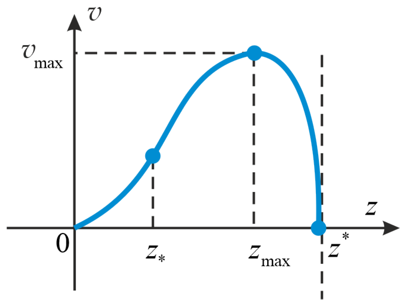
Returning to the plane of variables , we obtain that the separatrix S generates the solution to (26), shown in Figure 3, that satisfies the condition . The independent variable z here has its original meaning. The function initially increases with its first derivative, then the second derivative changes its sign at the point . Afterwards, reaches the maximum at the point , and changes its sign. Finally, at the point v again equals zero, and .
From the point of view of the original problem, the above means that solution (27) has two zero fronts, i.e., it is a function with finite support and geometrically represents a solitary wave. Moreover, the properties of the constructed solution differ from the previously obtained ones for the plane-symmetric case [36,37]. In particular, the first derivative for the studied solution to the ODE unexpectedly turned out to be non-monotonic.
6. Existence and Uniqueness Theorem
In this section, we formulate and prove the existence and uniqueness theorem for heat-wave-type solutions to Equation (4). Let us set the following boundary condition
Note that we considered the particular case , i.e., for a given zero front, and proved the existence and uniqueness theorem for a solution in the class of analytical functions [38].
Before formulating and proving the theorem, let us perform some auxiliary transformations. It is necessary since, unlike the previously studied problems, in Equation (4) the factor multiplying the square of the first derivative is not a constant, as in [37], and in (32) , as in [36].
We assume that the functions and are monotonic in some neighborhood of the initial time and sufficiently smooth. Then, we can swap the unknown function u for the independent variable , i.e., becomes a new unknown function. This procedure is a nonlinear analog of the hodograph transformation [8]. Equation (4) takes the form
It is not managed to linearize the equation, but the nonlinearities become more comprehensible. Boundary condition (32) takes the form
Previously, we applied a similar technique in the simpler case of power-law nonlinearity and without sources and sinks [40].
Recall that by analytical function, we mean a function of a real variable that coincides in some domain with its Taylor expansion.
Theorem 3.
Let
- 1.
- , are analytical functions in some neighborhood of the point and , , , .
- 2.
- , are analytical functions in some neighborhood of the point and , .
Proof.
The proof of Theorem 3 is divided into two stages. First, we construct a formal solution in the form of a multiple power series. Second, we prove its convergence by the majorant method. Let us introduce the notation
Before constructing, we also introduce new independent variables. Let
The subscript will be further omitted to simplify the notation. After substitution (35), problem (33), (34) takes the form
The coefficients of series (38) are determineed by induction of the total order of differentiation . We obtain from condition (37) including , . To find , we set in Equation (36). Taking into account the equality , we obtain the following cubic equation:
The zero root leads to the solution , which is meaningless from the point of view of the original formulation.
Let us consider two cases.
1. Assume . Then, Equation (34) has the zero root and two nonzero ones
According to the conditions of the theorem, the expression under the root is positive.
2. If (recall that and cannot simultaneously become zero), then
and we have the only non-zero root.
Each non-zero root corresponds to an analytical solution, i.e., there may be two or one. So, the base of induction is established.
Let us now make an induction hypothesis. Let all , have already been found. Now we are going to justify that the rest coefficients can be determined uniquely. Differentiating Equation (36) times with respect to t, k times with respect to s, , and taking into account the induction hypothesis, we arrive at the following system of linear algebraic equations (SLAE):
depend only on , where , i.e., they are known by the induction hypothesis. Their explicit form is cumbersome and not essential for further consideration.
Let us study system (40) to make sure that it is uniquely solvable. In fact, it can be rewritten in the following matrix form:
where , , , . It is easy to see that , . Simple calculations, albeit cumbersome ones, demonstrate that , meaning for all positive integers k.
If , the matrix of system (41) is tridiagonal, but there is no the diagonal dominance. If , then the matrix is bidiagonal. Next, we prove that its determinant is nonzero and solve (41).
The elements of sequences (42) are the principle minors of the matrix of system (41), and the following equality holds
One can easily make sure that for all n the following inequalities hold
Hence, the results show that ; in other words, SLAE (41) is consistent and has a unique solution.
If the upper limit of summation (multiplication) is less than the lower one, then the summand is considered equal to zero. Formula (43) is valid for any admissible , and in the case of , the first sum becomes zero.
Thus, series (38) is constructed. Moreover, in the case , the coefficients are determined in two ways; if , they are calculated uniquely.
Let us now proceed to the proof of the convergence of series (38). Two options are possible. First, we can perform direct estimates using Formula (43), as in [44]. However, this method is very time-consuming. Therefore, we prefer the second way and will construct the majorant problem as in [37]. The difference is that the current formulation is more complex and requires, as already noted, a transition to the hodograph plane.
Let us analyze series (38) when
Since is an analytical function in a neighborhood of and , then local convergence of series (38) in a neighborhood of implies local convergence of series (44) in a neighborhood of and vice versa.
Let us make a substitution of the unknown function . Then, Equation (33) takes the form
Since the convergence of series (44) has not yet been proven, we exclude from Equation (45) using the condition
which follows from (34). Differentiating (46) with respect to t gives us , which, in turn, transforms (45) into
For Equation (47) we consider the boundary condition
Problems (47) are (48) are equivalent to problems (33) and (34) due to the construction procedure. On the other hand, (47) and (48) are problems with specified heat wave fronts, which we have repeatedly considered earlier in simpler formulations. In this regard, the proof below is presented, briefly highlighting only the main points.
First, we introduce a new independent variable , which transform the curve into a coordinate axis. Second, we conduct partial Taylor expansions of the unknown function and the given functions included in (47):
Here, , , are known analytical functions of their arguments, and is a new unknown function. Then, problem (47), (48) takes the form
Here, are analytical functions of their arguments. Functions , are also analytical have the following proprties. and the rest depend on and derivatives of the function Z with respect to u up to order. The exact form of these functions is not given here, since it is not essential for the proof. Let us only note that . For Equation (49), we have the following initial condition:
Problem (49), (50) does not obey Lemma 2 from [45]; therefore, it has a unique non-zero analytical solution. The last steps are constructing a majorant problem and proving the existence of its analytical zero-dominant solution. These steps are carried out similarly as in [45] (see also [37]). □
Corollary 1.
If we consider solutions (38), constructed during the proof of Theorem 3, as implicit functions for , then together with the trivial solution , they form continuous solutions to problem (4), (32). Moreover, they have a heat-wave-type, series (44) set their fronts. The convergence of series (44) follows from the convergence of series (38).
Remark 4.
Remark 5.
The previously proven Theorems 1 and 2 are not special cases of Theorem 3.
Remark 6.
Example 1, in which , shows that the conditions of Theorem 3 are close to necessary ones.
7. Conclusions
Summing up, we note that the paper presents another significant step in the systematic research of diffusion-wave-type solutions to second-order nonlinear degenerate parabolic equations and systems. Such solutions are essential since they describe disturbances propagating over a stationary background with a finite velocity. This property allows us to describe heat, diffusion, and filtration processes occurring in physical, chemical, and biological systems. However, they differ dramatically from typical solutions to parabolic equations known for their instantaneous disturbance propagation. Such behavior of solutions is characteristic of hyperbolic equations. But in this case, it appears out of singularity associated with the vanishing of the higher derivative multiplier.
We consider a new formulation, construct and study exact solutions. Some of them are found in the explicit form, and the construction of the rest is reduced to the Cauchy problems for ODEs. Furthermore, we prove two existence and uniqueness theorems for solutions of the required type. The example we propose, an analog of Kovalevskaya’s classical result, deserves special attention. When the initial condition is a linear function, the properties of the solution turn out to be unexpected and emphasize the difference between the considered equation and its plane-symmetric analog.
Thus, we expand the previous results for the plane-symmetric case to a multidimensional (quasi-one-dimensional) one. The equation experiences a significant transformation. In particular, the origin becomes a singular point, so the direct transfer of methods and approaches here seems to be impossible. Therefore, we have to noticeably alter the technique. A new way of separating variables for constructing exact solutions is suggested. The main theorem requires transferring to the hodograph plane as well.
Further research in this direction may be related to developing computational algorithms for solving the problems considered. Since it is hardly ever possible to prove the convergence of numerical methods for degenerate nonlinear PDEs, the exact solutions found here, as well as segments of the series that are constructed when proving the theorems, can be used for verifying calculations. It is also helpful to evaluate the solution existence domain if it is impossible to obtain explicit formulas. A weighty result would be the weakening of the requirements for infinite smoothness of the input data, which, although fulfilled in the most natural cases, limits the generality of the consideration.
Finally, we note that our previous article [37] outlines a research plan, which involves considering cases when the unknown function depends on two or more spatial variables. The goal is to use the developed mathematical apparatus for solving applied problems related to diffusion processes modeling in Lake Baikal, which is included in the UNESCO World Heritage List. This work is the first step in implementation these plans.
Author Contributions
All authors contributed equally. All authors have read and agreed to the published version of the manuscript.
Funding
The research was funded by the Ministry of Science and Higher Education of the Russian Federation within the framework of the project “Analytical and numerical methods of mathematical physics in problems of tomography, quantum field theory, and fluid mechanics” (no. of state registration: 121041300058-1).
Institutional Review Board Statement
Not applicable.
Informed Consent Statement
Not applicable.
Data Availability Statement
No new data were created.
Conflicts of Interest
The authors declare no conflicts of interest.
References
- Friedman, A. Partial Differential Equations of Parabolic Type; Prentice-Hall: Englewood Cliffs, NJ, USA, 1964. [Google Scholar]
- Vazquez, J. The Porous Medium Equation: Mathematical Theory; Clarendon Press: Oxford, UK, 2007. [Google Scholar] [CrossRef]
- Samarskii, A.; Galaktionov, V.; Kurdyumov, S.; Mikhailov, A. Blow-Up in Quasilinear Parabolic Equations; Walter de Gruyte: Berlin, Germany, 1995. [Google Scholar] [CrossRef]
- Ladyzenskaja, O.; Solonnikov, V.; Ural’ceva, N. Linear and Quasi-Linear Equations of Parabolic Type. Translations of Mathematical Monographs, Vol. 23; American Mathematical Society: Providence, RI, USA, 1988. [Google Scholar]
- Grindrod, P. Patterns and Waves: Theory and Applications of Reaction-Diffusion Equations; Oxford Applied Mathematics and Computing Science Series; Clarendon Press: Oxford, UK, 1991. [Google Scholar]
- Boussinesq, J. Essai sur la Theorie des Eaux Courantes; Imprimerie Nationale: Paris, France, 1877. [Google Scholar]
- Evans, L. Partial Differential Equations; Graduate Studies in Mathematics; American Mathematical Society: Providence, RI, USA, 2010. [Google Scholar] [CrossRef]
- Courant, R.; Hilbert, D. Methods of Mathematical Physics. Vol. II: Partial Differential Equations; Interscience Publishers, Inc.: New York, NY, USA, 2008. [Google Scholar]
- Andreev, V.K.; Gaponenko, Y.A.; Goncharova, O.N.; Pukhnachev, V.V. Mathematical Models of Convection; Walter de Gruyte: Berlin, Germany, 2012. [Google Scholar] [CrossRef]
- Murray, J. Mathematical Biology: I. An Introduction, 3rd ed.; Interdisciplinary Applied Mathematics; Springer: New York, NY, USA, 2002; Volume 17. [Google Scholar] [CrossRef]
- Zeldovich, Y.B.; Raizer, Y.P. Physics of Shock Waves and High-Temperature Hydrodynamic Phenomena; Dover Publications: New York, NY, USA, 2002. [Google Scholar] [CrossRef]
- Barenblatt, G.; Entov, V.; Ryzhik, V. Theory of Fluid Flows Through Natural Rocks; Kluwer Academic Publishers: Dordrecht, The Netherlands, 1990. [Google Scholar]
- DiBenedetto, E. Degenerate Parabolic Equations; Springer: New York, NY, USA, 1993. [Google Scholar] [CrossRef]
- Chetverushkin, B.; Olkhovskaya, O.; Gasilov, V. An explicit difference scheme for non-linear heat conduction equation. Mat. Model. 2022, 34, 3–19. [Google Scholar] [CrossRef]
- Cassol, G.O.; Dubljevic, S. Hyperbolicity of the heat equation. IFAC-PapersOnLine 2019, 52, 63–67. [Google Scholar] [CrossRef]
- Sidorov, A.F. Analytic representations of solutions of nonlinear parabolic equations of time-dependent filtration type. Sov. Math. Dokl. 1985, 31, 40–44. [Google Scholar]
- Filimonov, M.Y.; Korzunin, L.G.; Sidorov, A.F. Approximate Methods for Solving Nonlinear Initial Boundary-Value Problems Based on Special Constructions of Series. Russ. J. Numer. Anal. Math. Model. 1993, 8, 101–126. [Google Scholar] [CrossRef]
- Filimonov, M.Y. Representation of solutions of boundary value problems for nonlinear evolution equations by special series with recurrently calculated coefficients. J. Phys. Conf. Ser. 2019, 1268, 012071. [Google Scholar] [CrossRef]
- Rubina, L.I.; Ul’yanov, O.N. On some method for solving a nonlinear heat equation. Sib. Math. J. 2012, 53, 872–881. [Google Scholar] [CrossRef]
- Polyanin, A.D.; Zhurov, A.I. Separation of Variables and Exact Solutions to Nonlinear PDEs; Chapman and Hall/CRC: Boca Raton, FL, USA, 2021. [Google Scholar] [CrossRef]
- Kudryashov, N.A.; Chmykhov, M.A. Approximate solutions to one-dimensional nonlinear heat conduction problems with a given flux. Comput. Math. Math. Phys. 2007, 47, 107–117. [Google Scholar] [CrossRef]
- Kudryashov, N.; Zakharchenko, A. A note on solutions of the generalized Fisher equation. Appl. Math. Lett. 2014, 32, 53–56. [Google Scholar] [CrossRef]
- Kudryashov, N.; Zakharchenko, A. Painlevé analysis and exact solutions of a predator–prey system with diffusion. Math. Methods Appl. Sci. 2015, 38, 1418–1427. [Google Scholar] [CrossRef]
- Sinelshchikov, D.I.; Kudryashov, N.A. Integrable Nonautonomous Lienard-Type Equations. Theor. Math. Phys. 2018, 196, 1230–1240. [Google Scholar] [CrossRef]
- Galaktionov, V.A.; Shishkov, A.E. Self-similar boundary blow-up for higher-order quasilinear parabolic equations. Proc. R. Soc. Edinb. Sect. A Math. 2005, 135, 1195–1227. [Google Scholar] [CrossRef]
- Stepanova, E.V.; Shishkov, A.E. Initial evolution of supports of solutions of quasilinear parabolic equations with degenerate absorption potential. Mat. Sb. 2013, 204, 79–106. [Google Scholar] [CrossRef]
- Shishkov, A.E.; Yevgenieva, Y.A. Localized Blow-Up Regimes for Quasilinear Doubly Degenerate Parabolic Equations. Math. Notes 2019, 106, 639–650. [Google Scholar] [CrossRef]
- Bui, D.; Nguyen, H.; Qin, X.; Wang, Y. On maximal solution to a degenerate parabolic equation involving in time fractional derivative. Electron. J. Appl. Math. 2023, 1, 62–80. [Google Scholar] [CrossRef]
- Gurefe, Y.; Le, D.L.; Kumar, D. Regularization of nonlocal pseudo-parabolic equation with random noise. Electron. J. Appl. Math. 2023, 1, 40–61. [Google Scholar] [CrossRef]
- Antontsev, S.; Shmarev, S. Evolution PDEs with Nonstandard Growth Conditions. Existence, Uniqueness, Localization, Blow-Up; Atlantis Press: Paris, France, 2015. [Google Scholar] [CrossRef]
- Antontsev, S.; Shmarev, S. Global Estimates for Solutions of Singular Parabolic and Elliptic Equations with Variable Nonlinearity. Nonlinear Anal.-Theory Methods Appl. 2020, 195, 111724. [Google Scholar] [CrossRef]
- Feo, F.; Vázquez, J.L.; Volzone, B. Anisotropic p-Laplacian Evolution of Fast Diffusion Type. Adv. Nonlinear Stud. 2021, 21, 523–555. [Google Scholar] [CrossRef]
- Feo, F.; Vázquez, J.L.; Volzone, B. Anisotropic fast diffusion equations. Nonlinear Anal. 2023, 233, 113298. [Google Scholar] [CrossRef]
- Vazquez, J.L. Asymptotic behaviour for the porous medium equation posed in the whole space. J. Evol. Equ. 2003, 3, 67–118. [Google Scholar] [CrossRef]
- Carrillo, J.A.; Gomez-Castro, D.; Vazquez, J.L. Infinite-time concentration in aggregation–diffusion equations with a given potential. J. Math. Pures Appl. 2022, 157, 346–398. [Google Scholar] [CrossRef]
- Kazakov, A. Solutions to Nonlinear Evolutionary Parabolic Equations of the Diffusion Wave Type. Symmetry 2021, 13, 871. [Google Scholar] [CrossRef]
- Kazakov, A.; Lempert, A. Diffusion-Wave Type Solutions to the Second-Order Evolutionary Equation with Power Nonlinearities. Mathematics 2022, 10, 232. [Google Scholar] [CrossRef]
- Kazakov, A.L. On exact solutions to a heat wave propagation boundary-value problem for a nonlinear heat equation. Sib. Electron. Math. Rep. 2019, 16, 1057–1068. [Google Scholar] [CrossRef]
- Kazakov, A.; Spevak, L. Constructing Exact and Approximate Diffusion Wave Solutions for a Quasilinear Parabolic Equation with Power Nonlinearities. Mathematics 2022, 10, 1559. [Google Scholar] [CrossRef]
- Kazakov, A.L.; Nefedova, O.A.; Spevak, L.F. Solution of the Problem of Initiating the Heat Wave for a Nonlinear Heat Conduction Equation Using the Boundary Element Method. Comput. Math. Math. Phys. 2019, 59, 1015–1029. [Google Scholar] [CrossRef]
- Kozlov, V.V. Sofya Kovalevskaya: A mathematician and a person. Russ. Math. Surv. 2000, 55, 1175–1192. [Google Scholar] [CrossRef]
- Andronov, A.A.; Leontovich, E.A.; Gordon, I.I.; Maier, A.G. Qualitative Theory of Second-Order Dynamic Systems; Israel Program for Scientific Translations; Halstead Press: Jerusalem, Israel, 1973. [Google Scholar]
- El-Mikkawy, M.E. On the inverse of a general tridiagonal matrix. Appl. Math. Comput. 2004, 150, 669–679. [Google Scholar] [CrossRef]
- Kazakov, A.; Lempert, A. Existence and Uniqueness of the Solution of the Boundary-Value Problem for a Parabolic Equation of Unsteady Filtration. J. Appl. Mech. Tech. Phys. 2013, 54, 251–258. [Google Scholar] [CrossRef]
- Kazakov, A.L.; Kuznetsov, P.A. On the Analytic Solutions of a Special Boundary Value Problem for a Nonlinear Heat Equation in Polar Coordinates. J. Appl. Ind. Math. 2018, 812, 227–235. [Google Scholar] [CrossRef]
Figure 1.
Heat wave.

Figure 2.
Phase portrait.
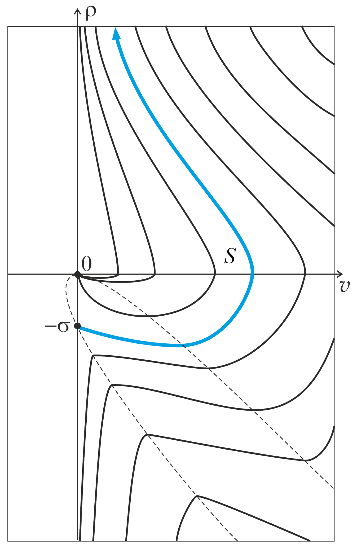
Figure 3.
Solution corresponding to S.
Disclaimer/Publisher’s Note: The statements, opinions and data contained in all publications are solely those of the individual author(s) and contributor(s) and not of MDPI and/or the editor(s). MDPI and/or the editor(s) disclaim responsibility for any injury to people or property resulting from any ideas, methods, instructions or products referred to in the content. |
© 2024 by the authors. Licensee MDPI, Basel, Switzerland. This article is an open access article distributed under the terms and conditions of the Creative Commons Attribution (CC BY) license (https://creativecommons.org/licenses/by/4.0/).
Share and Cite
MDPI and ACS Style
Kazakov, A.; Lempert, A. Multidimensional Diffusion-Wave-Type Solutions to the Second-Order Evolutionary Equation. Mathematics 2024, 12, 354. https://doi.org/10.3390/math12020354
AMA Style
Kazakov A, Lempert A. Multidimensional Diffusion-Wave-Type Solutions to the Second-Order Evolutionary Equation. Mathematics. 2024; 12(2):354. https://doi.org/10.3390/math12020354
Chicago/Turabian StyleKazakov, Alexander, and Anna Lempert. 2024. "Multidimensional Diffusion-Wave-Type Solutions to the Second-Order Evolutionary Equation" Mathematics 12, no. 2: 354. https://doi.org/10.3390/math12020354
Note that from the first issue of 2016, this journal uses article numbers instead of page numbers. See further details here.