
Stability and Synchronization of Delayed Quaternion-Valued Neural Networks under Multi-Disturbances
1
Vehicle Measurement, Control and Safety Key Laboratory of Sichuan Province, Xihua University, Chengdu 610039, China
2
Provincial Engineering Research Center for New Energy Vehicle Intelligent Control and Simulation Test Technology of Sichuan, Xihua University, Chengdu 610039, China
3
School of Mechanical Engineering, Xihua University, Chengdu 610039, China
4
College of Mechanical and Electrical Engineering, Qingdao University, Qingdao 266071, China
*
Author to whom correspondence should be addressed.
Mathematics 2024, 12(6), 917; https://doi.org/10.3390/math12060917
Submission received: 11 January 2024
/
Revised: 10 March 2024
/
Accepted: 15 March 2024
/
Published: 20 March 2024
(This article belongs to the Section Dynamical Systems)
Abstract
:This paper discusses a type of mixed-delay quaternion-valued neural networks (QVNNs) under impulsive and stochastic disturbances. The considered QVNNs model are treated as a whole, rather than as complex-valued neural networks (NNs) or four real-valued NNs. Using the vector Lyapunov function method, some criteria are provided for securing the mean-square exponential stability of the mixed-delay QVNNs under impulsive and stochastic disturbances. Furthermore, a type of chaotic QVNNs under stochastic and impulsive disturbances is considered using a previously established stability analysis method. After the completion of designing the linear feedback control law, some sufficient conditions are obtained using the vector Lyapunov function method for determining the mean-square exponential synchronization of drive–response systems. Finally, two examples are provided to demonstrate the correctness and feasibility of the main findings and one example is provided to validate the use of QVNNs for image associative memory.
1. Introduction
Neural networks (NNs) have been extensively used in medicine, biology, communication, and transportation because of their characteristics, such as nonlinear mapping, associative memory, classification and recognition, optimal computing, and others. A quaternion is a four-element vector in the class of hypercomplex numbers first described by Hamilton in 1843 [1]. Because a quaternion with one real and three imaginary parts can carry large amounts of information, it can handle multidimensional issues, such as associative memory for colored images [2], trajectory tracking control of a rotor missile [3], attitude and altitude tracking of a quadrotor unmanned aerial vehicle [4], and cross-modal matching [5] more effectively. Considering image associative memory as an example, a color image can be depicted by a quaternion matrix with pure imaginary numbers of suitable dimensionality, where the three imaginary parts correspond to the three basic monochromatic colors of red (R), green (G), and blue (B) in the RGB color space. This demonstrates that a quaternion matrix can hold more data than a real or complex matrix. Accordingly, a quaternion-valued neural network (QVNN) model is proposed. QVNNs combine the benefits of NNs and quaternions and outperform real-valued NNs and complex-valued NNs in solving three-dimensional and four-dimensional data problems; therefore, they have attracted considerable research interest [2,4,6,7,8,9,10,11,12,13,14,15,16,17,18,19,20,21,22,23,24,25,26,27,28,29].
During the implementation of NNs, the delay phenomenon is inevitable owing to the limitation of the switching speed of the amplifier or the signal transmission speed. The delay phenomenon may reduce the convergence rate to equilibria of NNs and even cause considerable damage to the stability of systems. The delay phenomena of NN models have been examined in the literature, including fixed delays [30], variable delays [9,10,11,12,13,21,22,23,24,25,26,31,32,33,34,35,36], infinitely distributed delays [21,33,34,36], and neutral delays [12]. Uncertain interference factors are also unpreventable in NNs. Impulsive and stochastic disturbances are two types of interference factors that are commonly found in practical systems, and they considerably degrade the system’s stability. Therefore, incorporating them into NN models when examining the dynamic behavior of NNs is imperative. In [13], an impulsive disturbed QVNN with time-varying delays was built. By decomposing the QVNNs into the equivalent real-valued NNs, the exponential stability conditions of the delayed system were derived using generalized norms. After stochastic disturbances were introduced into these models, and without decomposing QVNNs, the researchers of [12] obtained relevant criteria to ensure the mean-square stability of equilibria of a type of QVNNs with variable delays and neutral delays using the fixed-point theorem.
Because synchronization of nonlinear complex systems can be applied to image encryption, secure communication, associative memory, and many other fields [8], research on the synchronization of these systems has always been a priority. Synchronization has attracted considerable research interest in recent years because it is an important dynamic behavior of coupled chaotic NNs. Similar to the equilibria stability of NNs, the delay phenomenon [6,7,8,15,16,17,19,20,28,29,37,38,39,40,41,42,43,44,45,46,47,48], impulsive disturbances [6,14,27], and stochastic disturbances [38,39,40,43,44,45,46,48,49,50,51,52,53] should be considered when examining the synchronization control of chaotic NNs. Currently, most research results [37,38,39,40,41,42,43,44,45,46,47,48,49,50,51,53,54,55] on synchronization control are primarily applicable to NNs in the real number domain. However, research [6,7,8,14,15,16,17,18,19,20,27,28,29] on the synchronization control of NNs in the quaternion domain is scarce. Studies [8,14,27,56] have only considered impulsive disturbances when analyzing the synchronization of QVNNs. Other related studies [15,16,17,18,19,20,28,29] have not considered the influence of uncertain interference factors on synchronization control.
Based on the abovementioned analysis of the existing literature, it is concluded that:
- (1)
- Considering the existing uncertain QVNNs, studies [8,14,27,56] only considered impulsive disturbances, and the researchers of [12,57] only investigated stochastic disturbances. Furthermore, the stochastic disturbance introduced in the QVNNs in [12] does not exert any influence on connecting neurons.
- (2)
- Decomposition is a common method when dealing with multivalued NNs. Studies [7,9,10,11,13,14,19,20,21,23,24,25,26,27] decomposed QVNNs and proposed relevant criteria to ensure system stability or synchronization. However, decomposable quaternion activation functions are rare, and the assumptions associated with decomposable activation functions are strict.
- (3)
- The scalar Lyapunov function method is the most commonly used method for investigating the stability and synchronization of NNs [6,7,8,10,11,13,14,15,16,17,18,19,31,32,33,34,35,36,37,38,39,40,41,42,43,44,45,46,47,48,49,50,51,52,53,54,55,57]. Compared with vector Lyapunov functions, scalar Lyapunov functions are difficult to construct using this method.
- (4)
- The synchronization analysis of chaotic NNs based on the concept of the drive-response system is equivalent to the stability problem of a synchronization error system. Only a few studies have simultaneously investigated the stability and synchronization of QVNNs.
- (5)
To sum up, additional research on the dynamic behavior of delayed QVNNs under stochastic and impulsive disturbances is required. Therefore, we further investigate the aforementioned issues. The main contributions and advantages of this study are as follows:
- (1)
- We will consider both impulsive and stochastic disturbances in mixed-delay QVNNs and examine the interaction of connected neurons after introducing stochastic disturbances.
- (2)
- The non-decomposition method, which retains the coupling characteristics of each part of the quaternion, is used to conduct the research.
- (3)
- To avoid the difficulty of constructing the scalar Lyapunov functions, this study combines the vector Lyapunov function method with mathematical induction and differential integration theory and proposes sufficient criteria to ensure the mean-squared exponential stability of the equilibria of the system.
- (4)
- For a type of chaotic QVNNs with mixed delays as well as impulsive and stochastic disturbances, judgment conditions for ensuring the mean-square exponential synchronization of the drive-response system with a linear feedback controller are obtained using the established mean-square exponential stability conditions.
- (5)
- In this study, the correctness and feasibility of the stability and synchronization criteria are demonstrated in examples 1 and 2, respectively. Furthermore, the applicability of the criterion for realizing image associative memory is validated via example 3.
This paper comprises six main sections. Section 2 presents a description of the model and the associated assumptions. Section 3 and Section 4 present theorems and corollaries related to stability and synchronization judgments of QVNNs. Section 5 presents three simulation examples. Finally, conclusions and an outlook for future work are presented in Section 6.
Table 1 lists some symbols used in this paper.
2. Model Description and Preliminaries
A type of QVNNs with mixed delays as well as impulsive and stochastic disturbances is presented in this section, which can be expressed as follows:
where: denotes the state of the m-th neuron, , and n denotes the number of neurons. represents an abrupt change in the system state at a discrete time , . The discrete set satisfies , and when . . and are the weight matrices of the system (1) for no delay, variable delays, and infinite distributed delays between neurons, respectively. The function signifies the intensity of stochastic disturbances among neurons. represents the Brown motion defined with natural filtration . indicates the external input of the system. , and represent activation functions of the system (1) for no delays, variable delays, and infinite distributed delays among neurons, respectively. The positive matrix denotes the self-feedback interconnected matrix.
Multiple assumptions are expressed for the system (1).
Assumption 1.
The following assumptions are made for the delay part of the system (1).
(i) The variable time delay in model (1) is a bounded function .
(ii) The kernel function : in the infinite distributed delay is a piecewise continuous function, and satisfies
Here is a continuous function on with and .
Assumption 2.
It is presumed that activation functions with in system (1) satisfy the Lipschitz condition, indicating that such that the inequalities are valid, here , .
Remark 1.
Note that the activation functions and with in the system (1) satisfy the Lipschitz condition. Only the notation f in the Assumption 2 is substituted by or h.
Here, let , , and .
Assumption 3.
Suppose
and
, , . Let
, where with implying an impulsive function. We assume that the inequalities are valid for all , . Let , .
Assumption 4.
There exist positive numbers
and such that all the weighted functions of the stochastic term with () satisfy the follow-up inequalities:
Here, we denote and .
Remark 2.
In studies [12,31,33,36,38,39,40,44,45,48,49,50,51,53,57], stochastic disturbances were introduced into several NNs. As per the interaction of stochastic disturbance on each neuron, the function in (1) can be split into strong-coupling forms [31,33,38,48,49,50,53] and weak-coupling types [36,40,44,45,51]. The research objects of the studies [31,33,36,38,39,40,44,45,48,49,50,51,53] are real-valued NNs. Reference [12] investigated the stability of a class of QVNNs with firmly coupled stochastic perturbations, but without considering the delay in the stochastic term. In this analysis, the assumption conditions for stochastic disturbances involve not only strong coupling but also delays. Obviously, Assumption 4 in this paper includes Hypothesis H2 in [12].
Let be the continuous function mapping from to , and be the original condition of the system (1), where and .
The equilibria of model (1) are denoted as .
Definition 1.
If there exist constants and such that hold for external input , the equilibria of system (1) are mean-square exponential stability,
- where:
Lemma 1
([58]). For a differentiable quaternionic function , the formula is valid.
Lemma 2
is supposed an
process with second-order derivative respect to z(t), then
Here is estimated using . = . = = 0 and . .
Remark 3.
After substituting (4) into (5) and using Lemma 2, Equation (6) can be derived, which will be employed in the subsequent proof of the theorems,
Lemma 3
([21]). Let be a matrix . If the original parts of all eigenvalues in B are positive, then the conclusion that B is an M-matrix is consistent with the conclusion that there is a positive vector such that .
3. Main Results of Stability
Let . Accordingly, the system (1) is rewritten as follows:
where:
The initial condition of the system (7) is , , .
Apparently, the mean-square exponential stability of the zero solution of system (7) indicates that the equilibria of system (1) show mean-square exponential stability. In what follows, a theorem is suggested to determine the mean-square exponential stability of the equilibria of (1).
Theorem 1.
Suppose that Assumptions 1–4 hold. Let . If there is a positive constant with and a positive number such that for all and , the following inequalities (8) hold; accordingly, the equilibria of system (1) are mean-square exponential stability, and the converge rate is ,
Proof.
Selecting the candidate vector the Lyapunov function is as follows:
When , according to Lemmas 1 and 2, we obtain:
In what follows, the differential form of (9) will be modified to the integral form. Based on the theory of stochastic differential equations [59], after integrating both sides of (9) are from t to for any , and calculating the mathematical expectation of (9), we derive:
Given that the mathematical expectation of process has continuity, Equation (10) can be determined using the properties of integral [59]. Furthermore, by using Holder inequality and Young inequality, we have:
Define curve
and set
When we have . Let , , , where is a constant. Then
which means , , .
Furthermore, inequalities are necessarily valid, here and . If does not hold, then there will be some at the time instant , such that , and , here . By substituting these assumptions in (9) and considering (7), the following is obtained:
The preceding analysis disproves the assumption . Furthermore, we have , which equals to
Next, according to mathematical induction, we prove the follow-up inequalities (13) hold:
When , it follows from (12) that holds for , , where .
Suppose the follow-up inequalities (14) are true, then
When using Assumption 2, we derive:
Because inequalities (14) are modified as follows:
Therefore, it is also possible that the following inequalities exist:
The proof by contradiction method will be used to demonstrate that inequalities (17) are true. If inequalities (17) do not hold, there will be some and time instant , in which , equality (18) and inequalities (19) hold,
Substituting equality (18) and inequalities (19) into inequalities (11), and considering inequalities (9), we obtain
This conclusion is inconsistent with the assumption . Therefore, we can deduce that inequalities (17) are always true for all , , .
According to the mathematical induction method, we derive that the inequalities (21) hold,
It follows from the condition in Theorem 1 that , . Substituting it into inequalities (21), we obtain
Furthermore, for all , , , we obtain
which denotes hold, where .
Based on Definition 1, we can infer that the solution of system (7) demonstrates mean-square exponential stability. That implies that the equilibria of system (1) are exponentially stable in the mean square. □
When only stochastic disturbances are evaluated in the model (1), and no impulsive disturbances are considered, the corresponding corollary can be derived as follows.
Corollary 1.
Suppose that Assumptions 1, 2, and 4 hold. If for all and , the matrix is an M-matrix, then the equilibria of system (1) are mean-square exponential stability,
Proof.
Because is an M-matrix, it follows from Lemma 3 that there is a positive vector such that all inequalities (22) hold,
The functions related to the system (1) are constructed as follows:
It is evident that is a continuous function on , , . Therefore, there is a constant such that () holds. The left part of the proof for Corollary 1 can be obtained directly using the same procedure as that used for proving Theorem 1. □
When only impulsive disturbances are incorporated in model (1) and no stochastic disturbances are considered, the corresponding corollary is as follows.
Corollary 2.
Suppose that Assumptions 1–3 hold. Let
, . If there is a positive constant
with
and a positive number
such that for all
and
, the following inequalities hold, then the equilibria
of system (1) are exponentially stable, and the converge rate is
,
Because Corollary 2 can be obtained directly by proving Theorem 1 in a similar manner, we skip the proof of Corollary 2.
When there is no disturbance in model (1), the corollary is as follows.
Corollary 3.
It is supposed that Assumptions 1 and 2 hold. If the matrix is an M-matrix, where , , , then the equilibria of system (1) show exponential stability for all .
Remark 4.
Selecting an activation function is one of the most difficult problems in studying the dynamic behavior of NNs. Currently, boundedness and the Lipschitz conditions are the two most common assumptions. In studies [31,32,35,37,42,45,46,47,51] and [10], the activation functions are assumed to be in the real number field and quaternion field, respectively. In studies [30,33,36,38,39,41,43,44,48,49,53] and [14,15,16,17,18,19,20,21,22,26,29,34], the activation functions are assumed to meet the Lipschitz condition in the real field and quaternion field, respectively. Table 2 summarizes the review of existing work. According to this table, the existing results that the activation function satisfies the boundedness are very rare among the research results on the dynamic behavior of QVNNs.
Table 2 illustrates that almost no study has been conducted on the dynamic behavior of QVNNs using the non-decomposition method under the assumption that the quaternion activation function satisfies boundedness. Subsequently, Assumption 5 is used when the activation function in model (1) satisfies boundedness.
Assumption 5.
The neuron activation functions with in the system (1) satisfy the condition for any , , where the and are constants.
Remark 1 also applies to Assumption 5; therefore, we exclude it herein.
Remark 5.
Note that the constants
and
in Assumption 5 are allowed to be positive, negative, or zero. If we take
, Assumption 5 implies that
. The previously employed Lipschitz condition can be considered as a unique case of Assumption 5. According to this, we can directly derive the stability criteria when the activation function satisfies Assumption 5. The corresponding stability criteria will not be replicated here.
4. Main Results of Synchronization
As stated earlier, the synchronization control problem of chaotic systems can be modified into a stability problem of synchronization error systems to be analyzed. In this section, we will implement the stability study method presented in Section 3 to assess the mean square exponential synchronization problem by developing a linear feedback controller for a class of chaotic QVNNs with mixed time delays, stochastic disturbances, and impulsive disturbances.
First, the models are provided for chaotic QVNNs based on the drive-response conception.
The drive systems of chaotic QVNNs are defined as follows:
The response systems of chaotic QVNNs are described as follows:
In systems (25) and (26), and denote the neuronal states of the drive system and the response system, respectively, and denotes the driving signal or synchronous control signal of the response system. The definitions of other symbols and functions are entirely coherent with the relevant definitions in system (1), which are excluded here.
The synchronization error signal is characterized as , . The synchronization errors of drive-response systems are expressed as (27),
where:
Here, we use the coupling of each neuron output signal as the synchronization control signal in the following form:
Let:
The definition of mean-square exponential synchronization is stated below.
Definition 2.
The response state of system (26) is exponentially synchronized in the mean square sense with the drive state of system (25) under the control signal with the form of (28), if there are constants and such that hold,
where
here .
By substituting (28) into (27), the error of the synchronization system is rewritten as follows:
Remark 6.
As an extended application of Theorem 1, assume that the delay parts of the error system (29) satisfy Assumption 1, the activation functions , and satisfy Assumption 2, the impulsive parts satisfy Assumption 3, and the stochastic coupling functions satisfy Assumption 4.
Theorem 2.
Suppose that Assumptions 1–4 hold. Let . If there is a positive constant with and a positive number such that the follow-up inequalities (30) hold, then the response state of system (26) can determine mean-square exponential synchronization with the drive state of system (25) under the control signal designed as (28), and the converge rate of synchronization error system is ,
Proof.
Selecting vector Lyapunov functions as follows:
When , according to Lemmas 1 and 2, we obtain:
Subsequently, the differential form of (31) is transposed to the integral form. Based on the theory of stochastic differential equations [59], after integrating both sides of (31) are from t to for any and calculating the expectation of (31), we obtain:
Given that the math expectation of process has continuity, Equation (32) can be determined using the properties of integral [59]. Furthermore, by using Holder inequality and Young inequality, we have:
The other part of the proof of Theorem 2 conforms with Theorem 1; therefore, it is omitted herein.
Furthermore, we can determine that the follow-up conclusion covers all , , ,
which implies
where and .
Definition 2 infers that the zero solution of the error system (29) demonstrates mean-square exponential stability, which indicates that the neuron of drive system (25) can be exponentially synchronized in the mean-square sense with the neuron of response system (26). □
Because Corollary 1–3 regarding the stability discussion in section three applies to the synchronization discussion as well, it will not be restated here.
Notably, most researchers [6,7,8,10,11,13,14,15,16,17,18,19,31,32,33,34,35,36,37,38,39,40,41,42,43,44,45,46,47,48,49,50,51,52,53,54,55,57] have used the scalar Lyapunov function method for the stability analysis of the synchronization error of chaotic NNs. By observing the scalar Lyapunov functions constructed in literature [6,7,8,10,11,13,14,15,16,17,18,19,31,32,33,34,35,36,37,38,39,40,41,42,43,44,45,46,47,48,49,50,51,52,53,54,55,57], it is clear that the form of the scalar Lyapunov function is rather complicated. In addition, when the system being analyzed is an infinite dimensional system, the convergence of the scalar Lyapunov function must be analyzed first, which leads to a complicated research process. The vector Lyapunov function method with simple forms is employed herein to investigate infinite dimensional error systems (27) in a manner that avoids the convergence analysis of this function.
5. Examples
5.1. Example 1
Consider the following system:
It is assumed that the quaternion matrices are as follows:
Here, let the delays in the model (34) be , , , and . Let and .
Let:
After computation, we acquire , . , , .
After substituting the above-assumed conditions into (8), we acquire , , which implies that Theorem 1 holds. Based on Theorem 1, the zero solution of the model (34) shows mean-square exponential stability, and the convergence rate is .
Furthermore, we estimate that the matrix outlined in Corollary 3 is . Evidently, the matrix is an M-matrix, and thus Corollary 3 holds.
As the external inputs in the model (34) are , it follows from Theorem 1 that the equilibria of the system (34) are zero with mean-square exponential stability. The state trajectories of and in model (34) without and with disturbances are depicted in Figure 1 and Figure 2 with the same initial conditions and , respectively. Figure 1 shows that the equilibria of the system (34) without disturbances are zero solution and unique, and that these equilibria are convergent. When there are impulsive disturbances and stochastic disturbances in the system (34), it can be seen from Figure 2 that the equilibria of system (34) converge to zero, but the convergence speed becomes slower relative to that shown in Figure 1. The simulation results prove the correctness of Theorem 1.
5.2. Example 2
Considering the following chaotic QVNNs as a drive system:
Considering the following chaotic QVNNs as a response system:
Let . The following are believed to be the interconnected matrices and control parameters:
Furthermore, the other parameters of the systems (35) and (36) are consistent with those of the system (34).
After substituting the above-assumed conditions into inequality (8), we acquire and . Based on verification, the conditions of Theorem 2 hold. It follows from Theorem 2 that the mean square exponential synchronization of the drive and response systems can be realized, and the convergence rate is .
The initial conditions of the drive system (35) and response system (36) are , , and , here .
When there are no disturbances, the phase plane of drive system (35) shows that the states of system (35) are in chaos (Figure 3). The state trajectories of the response and drive systems with impulsive and stochastic disturbances as well as their error curves are depicted in Figure 4 and Figure 5, where the blue and red curves represent the state curves of the drive and response systems, respectively, and the black curves represent their synchronization error curves. The error curves shown in Figure 4 and Figure 5 show that the response system will eventually synchronize with the drive system, which further verifies the correctability of the synchronization determination conditions established in Theorem 2.
5.3. Example 3
Here, a representative Lena image is selected for testing, which is widely used in image processing–related research owing to its complete inclusion of flat areas, shadows, textures and other details. The original Lena image used is shown in Figure 6, which is a color image with dimensions of 128 pixels × 128 pixels. Because of the limitation of the research group’s computer processing power, this study only evaluates time-varying delays and not the infinite distributed delays when designing QVNNs to implement color image associative memory. The designed model is defined as follows:
wherein: the activation functions are expressed as . It is assumed that , and the interconnected matrices are:
where .
As the associative memory process based on NNs is simulated on electronic devices, which is characterized by a complex structure as well as large amounts of data and calculation, the associative memory process will inevitably be affected by the impulsive disturbances of electronic devices, which will reduce the efficiency of the associative memory of the color image and even lead to erroneous associative memory results directly. Therefore, impulsive disturbances are considered in system (37).
Figure 6 comprises 128 pixels × 128 pixels = 16,384 pixels in total. When QVNNs are used for associative memory, each pixel corresponds to a neuron. The value of RGB three channels of each pixel is assigned to the three imaginary parts of the quaternion in turn, as the initial state of each neuron of QVNNs. For easy observation, we arbitrarily select the state curves of five neurons in model (37) to be shown, i.e., , , and . For subsequent comparison, Figure 7 shows the state curves of each part of the five neurons selected without considering any disturbances. As illustrated in Figure 7, the states of each neuron eventually shift to their equilibria, respectively. Notably, because the RGB requires only three parts of the quaternion, the three imaginary parts of the quaternion neuron are used in the simulation.
To compare the effects comprehensively, we conducted simulations for both cases of weak stochastic disturbances and strong stochastic disturbances. Here, it is assumed that where the intensity of the impulsive disturbance to each neuron is taken randomly in the interval of [1, 1.5], where and .
Case 1. Weak stochastic disturbances:
Taking , .
Case 2. Strong stochastic disturbances:
Taking , .
The simulations are depicted in Figure 8, Figure 9, Figure 10 and Figure 11, where Figure 8 (under the weak stochastic disturbances) and Figure 10 (under the strong stochastic disturbances) show the state curves of five randomly selected neurons, and Figure 9 (under the weak stochastic disturbances) and Figure 11 (under the strong stochastic disturbances) depict the image association memory process based on the designed QVNNs implemented in (37).
For case 1 (weak interference) and case 2 (strong interference), several simulation experiments demonstrate that the average PSNR value of case 2 is 11.1% lower than that of case 1 when the simulation time is taken as 20 s and the simulation step size is 0.1 s. This indicates that the greater the intensity of the stochastic disturbance, the greater the impact of QVNNs on the image associative memory. These simulation results further validate the correctness of the conclusions of this paper.
Remark 7.
The magnitude of stochastic disturbance strength exerts a direct effect on the undulation intensity of gray value data at each pixel in the image. The stronger the stochastic disturbance, the stronger the fluctuation of gray value data of each pixel in the image. However, it is difficult to directly observe the influence of stochastic disturbance strength on the quality of image restoration from the visual perspective of Figure 9 and Figure 11. To measure the effect of stochastic disturbance strength on the efficiency of image recovery during neural network associative memory, the peak signal noise ratio (PSNR), a frequently employed image evaluation metric, was selected to examine the image quality. The higher the value of PSNR, the closer the current image is to the original image. Table 3 demonstrates the recovery quality of the images at the corresponding moments in Figure 9 and Figure 11 for different stochastic disturbance strength through PSNR data. By comparing the PSNR data in Table 3, we conclude that: (1) the stability of the neural network in any of the three cases is not destroyed, and (2) the PSNR values in the strong stochastic disturbance case are lower than those in the weak stochastic disturbance case at the same moments.
6. Conclusions and Future Work
For a type of mixed-delay QVNNs with stochastic and impulsive disturbances, several conditions are proposed to determine the mean-square exponential stability of the system in light of the nondecomposition method. This research is being expanded to include the synchronization control of chaotic QVNNs using stochastic and impulsive disturbances. By designing a linear feedback controller and using the previously established stability analysis method, some sufficient conditions were obtained for realizing/determining the mean-square exponential synchronization of the drive–response system. The correctness and feasibility of the main results were validated using two numerical examples. Furthermore, the associative memory of color images by designing an appropriate QVNNs was achieved. Motivated by the studies [60,61,62], our approach in this paper will be applied to further discuss the stability of discrete QVNNs with variable coefficients and Markovian jumping parameters.
Author Contributions
Conceptualization, J.Y. and X.X.; methodology, Q.X. and X.X.; software, H.Y. and M.Y.; writing—original draft preparation, X.X., J.Y. and H.Y.; writing—review and editing, Q.X. and M.Y.; funding acquisition, J.Y. and X.X. All authors have read and agreed to the published version of the manuscript.
Funding
This work was supported by the Key Research and Development Project of Sichuan Province (grant numbers 2023YFG0067 and 2023YFG0068), the Key Programs of Sichuan Provincial Nature Fund (grant number 24NSFSC0043), the Open Project of State Key Laboratory of Industrial Control Technology (grant number ICT2022B45); and the ‘Chunhui Plan’ Cooperative Research for Ministry of Education (grant number 191657).
Institutional Review Board Statement
Not applicable.
Informed Consent Statement
Not applicable.
Data Availability Statement
Data will be made available on request.
Conflicts of Interest
The authors declare no conflicts of interest.
References
- Isokawa, T.; Kusakabe, T.; Matsui, N.; Peper, F. Quaternion neural network and its application. In Proceedings of the Knowledge-Based Intelligent Information and Engineering Systems, 7th International Conference, Berlin, Germany, 3 September 2003. [Google Scholar]
- Chen, X.F.; Song, Q.K.; Li, Z.S. Design and analysis of quaternion-valued neural networks for associative memories. IEEE Trans. Syst. Man Cybern. Syst. 2018, 49, 2305–2314. [Google Scholar] [CrossRef]
- Zhao, J.; Shi, Z.J.; Wang, Y.C.; Wang, W. Quaternion-based adaptive trajectory tracking control of a rotormissile with unknown parameters identification. Def. Technol. 2024, 31, 375–386. [Google Scholar] [CrossRef]
- Xian, B.; Diao, C.; Zhao, B.; Zhang, Y. Nonlinear robust output feedback tracking control of a quadrotor UAV using quaternion representation. Nonlinear Dyn. 2015, 79, 2735–2752. [Google Scholar] [CrossRef]
- Wang, Z.; Xu, X.; Wei, J.W.; Xie, N.; Shao, J.; Yang, Y. Quaternion representation learning for cross-modal matching. Knowl.-Based Syst. 2023, 270, 110505. [Google Scholar] [CrossRef]
- Yan, H.Y.; Qiao, Y.H.; Duan, L.J.; Miao, J. New inequalities to finite-time synchronization analysis of delayed fractional-order quaternion-valued neural networks. Neural Comput. Appl. 2022, 34, 9919–9930. [Google Scholar] [CrossRef]
- Aouiti, C.; Bessifi, M. Periodically intermittent control for finite-time synchronization of delayed quaternion-valued neural networks. Neural Comput. Appl. 2021, 33, 6527–6547. [Google Scholar] [CrossRef]
- Lin, D.Y.; Chen, X.F.; Yu, G.P.; Li, Z.S.; Xia, Y.N. Global exponential synchronization via nonlinear feedback control for delayed inertial memristor-based quaternion-valued neural networks with impulses. Appl. Math. Comput. 2021, 401, 126093. [Google Scholar] [CrossRef]
- Liu, Y.; Zhang, D.D.; Lu, J.Q. Global exponential stability for quaternion-valued recurrent neural networks with time-varying delays. Nonlinear Dyn. 2017, 87, 553–565. [Google Scholar] [CrossRef]
- Shu, J.L.; Wu, B.W.; Xiong, L.L. Stochastic stability criteria and event-triggered control of delayed Markovian jump quaternion-valued neural networks. Appl. Math. Comput. 2022, 420, 126904. [Google Scholar] [CrossRef]
- Shu, J.L.; Wu, B.W.; Xiong, L.L.; Wu, T.; Zhang, H.Y. Stochastic stabilization of markov jump quaternion-valued neural network using sampled-data control. Appl. Math. Comput. 2021, 400, 126041. [Google Scholar] [CrossRef]
- Song, Q.K.; Zeng, R.T.; Zhao, Z.J.; Liu, Y.R.; Alsaadi, F.E. Mean-square stability of stochastic quaternion-valued neural networks with variable coefficients and neutral delays. Neurocomputing 2022, 471, 130–138. [Google Scholar] [CrossRef]
- Wang, H.M.; Wei, G.L.; Wen, S.P.; Huang, T.W. Impulsive disturbance on stability analysis of delayed quaternion-valued neural networks. Appl. Math. Comput. 2021, 390, 125680. [Google Scholar] [CrossRef]
- Qi, X.N.; Bao, H.B.; Cao, J.D. Synchronization criteria for quaternion-valued coupled neural networks with impulses. Neural Netw. 2020, 128, 150–157. [Google Scholar] [CrossRef]
- Zhang, T.T.; Jian, J.G. Quantized intermittent control tactics for exponential synchronization of quaternion-valued memristive delayed neural networks. ISA Trans. 2021, 126, 288–299. [Google Scholar] [CrossRef]
- Li, R.X.; Cao, J.D.; Xue, C.F.; Manivannan, R. Quasi-stability and quasi-synchronization control of quaternion-valued fractional-order discrete-time memristive neural networks. Appl. Math. Comput. 2021, 395, 125851. [Google Scholar] [CrossRef]
- Zhang, J.S.; Ma, X.L.; Li, Y.K.; Gan, Q.T.; Wang, C.L. Synchronization in fixed/preassigned-time of delayed fully quaternion-valued memristive neural networks via non-separation method. Commun. Nonlinear Sci. Numer. Simul. 2022, 113, 106581. [Google Scholar] [CrossRef]
- Peng, T.; Zhong, J.; Tu, Z.W.; Lu, J.Q.; Lou, J.G. Finite-time synchronization of quaternion-valued neural networks with delays: A switching control method without decomposition. Neural Netw. 2022, 148, 37–47. [Google Scholar] [CrossRef]
- Wei, W.L.; Yu, J.; Wang, L.M.; Hu, C.; Jiang, H.J. Fixed/Preassigned-time synchronization of quaternion-valued neural networks via pure power-law control. Neural Netw. 2022, 146, 341–349. [Google Scholar] [CrossRef]
- Chen, Y.H.; Zhang, X.; Xue, Y. Global exponential synchronization of high-order quaternion hopfield neural networks with unbounded distributed delays and time-varying discrete delays. Math. Comput. Simul. 2022, 193, 173–189. [Google Scholar] [CrossRef]
- Xu, X.H.; Xu, Q.; Yang, J.B.; Xue, H.B.; Xu, Y.H. Further research on exponential stability for quaternion-valued neural networks with mixed delays. Neurocomputing 2020, 400, 186–205. [Google Scholar] [CrossRef]
- Zhang, Z.Q.; Yang, Z. Asymptotic stability for quaternion-valued fuzzy BAM neural networks via integral inequality approach. Chaos Soliton Fractals 2023, 169, 113227. [Google Scholar] [CrossRef]
- Xia, Y.N.; Chen, X.F.; Lin, D.Y.; Li, B.; Yang, X.J. Global exponential stability analysis of commutative quaternion-valued neural networks with time delays on time scales. Neural Process. Lett. 2023, 55, 6339–6360. [Google Scholar] [CrossRef]
- Chouhan, S.S.; Das, S.; Singh, S.; Shen, H. Multiple mu-stability analysis of time-varying delayed quaternion-valued neural networks. Math. Methods Appl. Sci. 2023, 46, 9853–9875. [Google Scholar] [CrossRef]
- Yu, S.Y.; Li, H.; Chen, X.F.; Lin, D.Y. Multistability analysis of quaternion-valued neural networks with cosine activation functions. Appl. Math. Comput. 2023, 445, 127849. [Google Scholar] [CrossRef]
- Tan, G.Q.; Wang, Z.S.; Shi, Z. Proportional–integral state estimator for quaternion-valued neural networks with time-varying delays. IEEE Trans. Neural Netw. Learn. Syst. 2023, 34, 1074–1079. [Google Scholar] [CrossRef]
- Mo, W.J.; Bao, H.B. Finite-time synchronization for fractional-order quaternion-valued coupled neural networks with saturated impulse. Chaos Soliton Fractals 2022, 164, 112714. [Google Scholar] [CrossRef]
- Kiruthika, R.; Krishnasamy, R.; Lakshmanan, S.; Prakash, M.; Manivannan, A. Non-fragile sampled-data control for synchronization of chaotic fractional-order delayed neural networks via LMI approach. Chaos Soliton Fractals 2023, 169, 113252. [Google Scholar] [CrossRef]
- Tao, P.; Wu, Y.Q.; Tu, Z.W.; Alofi, A.S.; Lu, J.Q. Fixed-time and prescribed-time synchronization of quaternion-valued neural networks: A control strategy involving Lyapunov functions. Neural Netw. 2023, 160, 108–121. [Google Scholar]
- Lv, X. A new approach to stability analysis for stochastic hopfield neural networks with time delays. IEEE Trans. Autom. Control 2022, 67, 5278–5288. [Google Scholar] [CrossRef]
- Yang, D.; Li, X.D.; Song, S.J. Design of state-dependent switching laws for stability of switched stochastic neural networks with time-delays. IEEE Trans. Neural Netw. Learn. Syst. 2020, 31, 1808–1819. [Google Scholar] [CrossRef]
- Chen, T.; Peng, S.G.; Hong, Y.H.; Mai, G.Z. Finite-time stability and stabilization of impulsive stochastic delayed neural networks with rous and rons. IEEE Access 2020, 8, 87133–87141. [Google Scholar] [CrossRef]
- Sheng, Y.; Zhang, H.; Zeng, Z.G. Stability and robust stability of stochastic reaction–diffusion neural networks with infinite discrete and distributed delays. IEEE Trans. Syst. Man Cybern. Syst. 2020, 50, 1721–1732. [Google Scholar] [CrossRef]
- Wang, L.M.; Ge, M.F.; Hu, J.H.; Zhang, G.D. Global stability and stabilization for inertial memristive neural networks with unbounded distributed delays. Nonlinear Dyn. 2019, 95, 943–955. [Google Scholar] [CrossRef]
- Tian, Y.F.; Wang, Z.S. Stochastic stability of markovian neural networks with generally hybrid transition rates. IEEE Trans. Neural Netw. Learn. Syst. 2022, 33, 7390–7399. [Google Scholar] [CrossRef]
- Liu, X.Z.; Wu, K.N.; Ding, X.H.; Zhang, W.H. Boundary stabilization of stochastic delayed cohen–grossberg neural networks with diffusion terms. IEEE Trans. Neural Netw. Learn. Syst. 2022, 33, 3227–3237. [Google Scholar] [CrossRef]
- Wei, Y.L.; Park, J.H.; Karimi, H.R.; Tian, Y.C.; Jung, H. Improved stability and stabilization results for stochastic synchronization of continuous-time semi-markovian jump neural networks with time-varying delay. IEEE Trans. Neural Netw. Learn. Syst. 2018, 29, 2488–2501. [Google Scholar] [CrossRef]
- Chen, L.J.; Wan, L.Y.; Wei, X.L.; Wang, L.M.; He, H.Q. Adaptive synchronization of reaction diffusion neural networks with infinite distributed delays and stochastic disturbance. IEEE Access 2020, 8, 180411–180421. [Google Scholar] [CrossRef]
- Chen, H.B.; Shi, P.; Lim, C.C. Exponential synchronization for markovian stochastic coupled neural networks of neutral-type via adaptive feedback control. IEEE Trans. Neural Netw. Learn. Syst. 2017, 28, 1618–1632. [Google Scholar] [CrossRef]
- Bao, H.B.; Park, J.H.; Cao, J.D. Exponential synchronization of coupled stochastic memristor-based neural networks with time-varying probabilistic delay coupling and impulsive delay. IEEE Trans. Neural Netw. Learn. Syst. 2016, 27, 190–201. [Google Scholar] [CrossRef]
- Zhang, X.L.; Li, H.L.; Kao, Y.G.; Zhang, L.; Jiang, H.J. Global mittag-leffler synchronization of discrete-time fractional-order neural networks with time delays. Appl. Math. Comput. 2022, 433, 127417. [Google Scholar] [CrossRef]
- Zhang, H.G.; Wang, J.Y.; Wang, Z.S.; Liang, H.J. Mode-dependent stochastic synchronization for markovian coupled neural networks with time-varying mode-delays. IEEE Trans. Neural Netw. Learn. Syst. 2015, 26, 2621–2634. [Google Scholar] [CrossRef]
- Li, X.F.; Bi, D.J.; Xie, X.; Xie, Y.L. Multi-synchronization of stochastic coupled multi-stable neural networks with time-varying delay by impulsive control. IEEE Access 2019, 7, 15641–15653. [Google Scholar] [CrossRef]
- Pan, L.J.; Song, Q.K.; Cao, J.D.; Ragulskis, M. Pinning impulsive synchronization of stochastic delayed neural networks via uniformly stable function. IEEE Trans. Neural Netw. Learn. Syst. 2021, 33, 4491–4501. [Google Scholar] [CrossRef]
- Wang, Q.J.; Zhao, H.; Liu, A.D.; Li, L.X.; Niu, S.J.; Chen, C. Predefined-time synchronization of stochastic memristor-based bidirectional associative memory neural networks with time-varying delays. IEEE Trans. Cogn. Dev. Syst. 2022, 14, 1584–1593. [Google Scholar] [CrossRef]
- Chen, G.L.; Xia, J.W.; Park, J.H.; Shen, H.; Zhuang, G.M. Sampled-data synchronization of stochastic markovian jump neural networks with time-varying delay. IEEE Trans. Neural Netw. Learn. Syst. 2022, 33, 3829–3841. [Google Scholar] [CrossRef]
- Yao, L.; Wang, Z.; Huang, X.; Li, Y.X.; Ma, Q.; Shen, H. Stochastic sampled-data exponential synchronization of markovian jump neural networks with time-varying delays. IEEE Trans. Neural Netw. Learn. Syst. 2023, 34, 909–920. [Google Scholar] [CrossRef]
- Cao, Z.R.; Li, C.D.; He, Z.L.; Zhang, X.Y.; You, L. Synchronization of coupled stochastic reaction-diffusion neural networks with multiple weights and delays via pinning impulsive control. IEEE Trans. Netw. Sci. Eng. 2022, 9, 820–833. [Google Scholar] [CrossRef]
- Zhou, W.N.; Zhu, Q.Y.; Shi, P.; Su, H.Y.; Fang, J.A.; Zhou, L.W. Adaptive synchronization for neutral-type neural networks with stochastic perturbation and markovian switching parameters. IEEE Trans. Cybern. 2014, 44, 2848–2860. [Google Scholar] [CrossRef]
- Yuan, J.X.; Zhang, C.; Chen, T. Command filtered adaptive neural network synchronization control of nonlinear stochastic systems with lévy noise via event-triggered mechanism. IEEE Access 2021, 9, 146195–146202. [Google Scholar] [CrossRef]
- Guo, Z.Y.; Xie, H.; Wang, J. Finite-time and fixed-time synchronization of coupled switched neural networks subject to stochastic disturbances. IEEE Trans. Syst. Man Cybern. Syst. 2022, 52, 6511–6532. [Google Scholar] [CrossRef]
- Liu, M.J.; Wang, X.R.; Zhang, Z.Y.; Wang, Z. Global synchronization of complex-valued neural networks with stochastic disturbances and time-varying delay. IEEE Access 2019, 7, 182600–182610. [Google Scholar] [CrossRef]
- Liang, T.; Yang, D.G.; Lei, L.; Zhang, W.L.; Pan, J. Preassigned-time bipartite synchronization of complex networks with quantized couplings and stochastic perturbations. Math. Comput. Simul. 2022, 202, 559–570. [Google Scholar] [CrossRef]
- Wang, H.Q.; Ai, Y.D. Adaptive fixed-time control and synchronization for hyperchaotic Lü systems. Appl. Math. Comput. 2022, 433, 127388. [Google Scholar] [CrossRef]
- Hu, Z.P.; Ren, H.R.; Shi, P. Synchronization of complex dynamical networks subject to noisy sampling interval and packet loss. IEEE Trans. Neural Netw. Learn. Syst. 2022, 33, 3216–3226. [Google Scholar] [CrossRef]
- Peng, T.; Lu, J.Q.; Xiong, J.; Tu, Z.W.; Liu, Y.; Lou, J.G. Fixed-time synchronization of quaternion-valued neural networks with impulsive effects: A non-decomposition method. Commun. Nonlinear Sci. Numer. Simul. 2024, 132, 107865. [Google Scholar] [CrossRef]
- Zeng, R.T.; Song, Q.K. Mean-square exponential input-to-state stability for stochastic neutral-type quaternion-valued neural networks via Itô’s formula of quaternion version. Chaos Soliton Fractals 2024, 178, 114341. [Google Scholar] [CrossRef]
- Xu, X.H.; Yang, J.B.; Yang, H.L.; Sun, S.L. Effect of impulses on robust exponential stability of delayed quaternion-valued neural networks. Neural Process. Lett. 2023, 55, 9615–9634. [Google Scholar] [CrossRef]
- Oksendal, B. Stochastic differential equations—An introduction with applications plications applications. In Springer Science & Business Media; Springer: Berlin/Heidelberg, Germany, 2013. [Google Scholar]
- Song, Q.K.; Yu, Q.Q.; Zhao, Z.J.; Liu, Y.R.; Alsaadi, F.E. Dynamics of complex-valued neural networks with variable coefficients and proportional delays. Neurocomputing 2018, 275, 2762–2768. [Google Scholar] [CrossRef]
- Jia, S.F.; Chen, Y.H. Discrete analogue of impulsive recurrent neural networks with both discrete and finite distributive asynchronous time-varying delays. Cogn. Neurodynamics 2022, 16, 733–744. [Google Scholar] [CrossRef] [PubMed]
- Cai, T.; Cheng, P.; Yao, F.Q.; Hua, M.G. Robust exponential stability of discrete-time uncertain impulsive stochastic neural networks with delayed impulses. Neural Netw. 2023, 160, 227–237. [Google Scholar] [CrossRef]
Figure 1.
Transient behavior of and in the system (34) without impulsive and stochastic disturbances.
Figure 1.
Transient behavior of and in the system (34) without impulsive and stochastic disturbances.
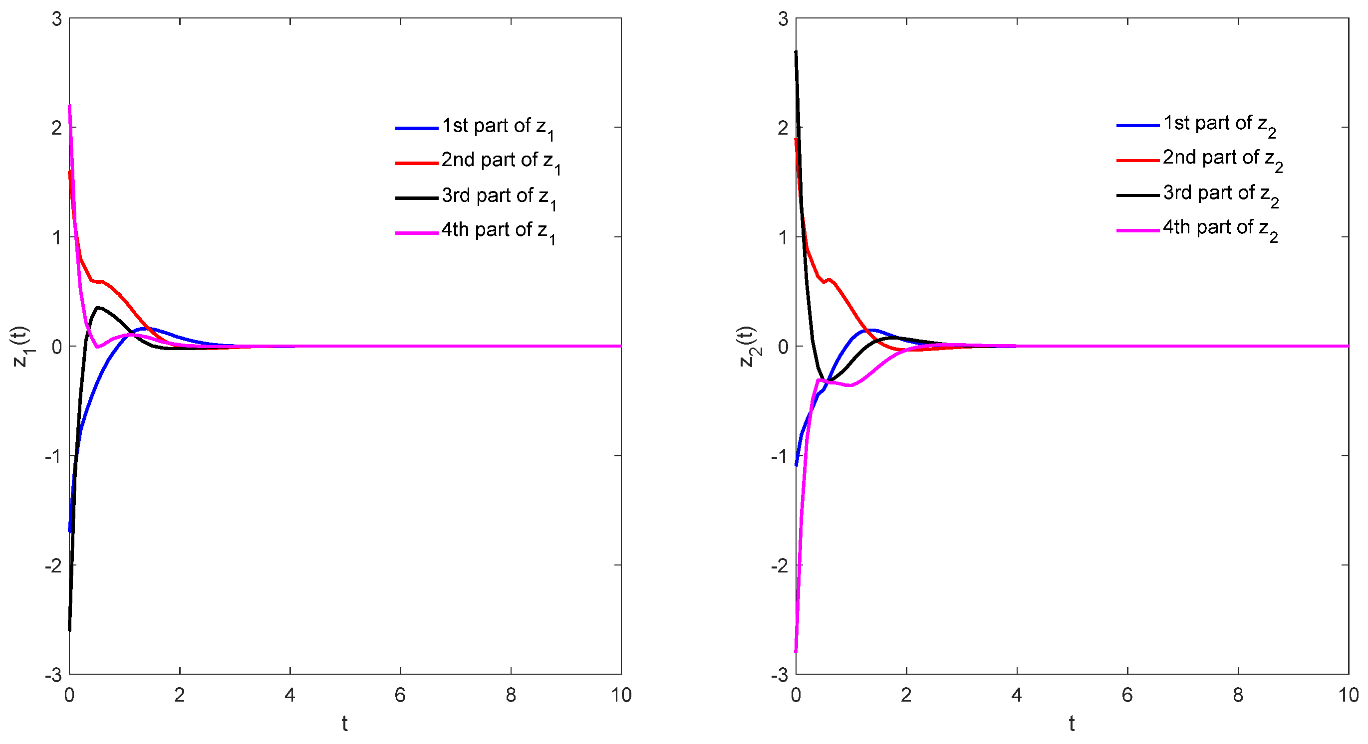
Figure 2.
Transient behavior of and in the system (34) with impulsive and stochastic disturbances.

Figure 3.
Phase plane of the drive system (35) without impulsive and stochastic disturbances.
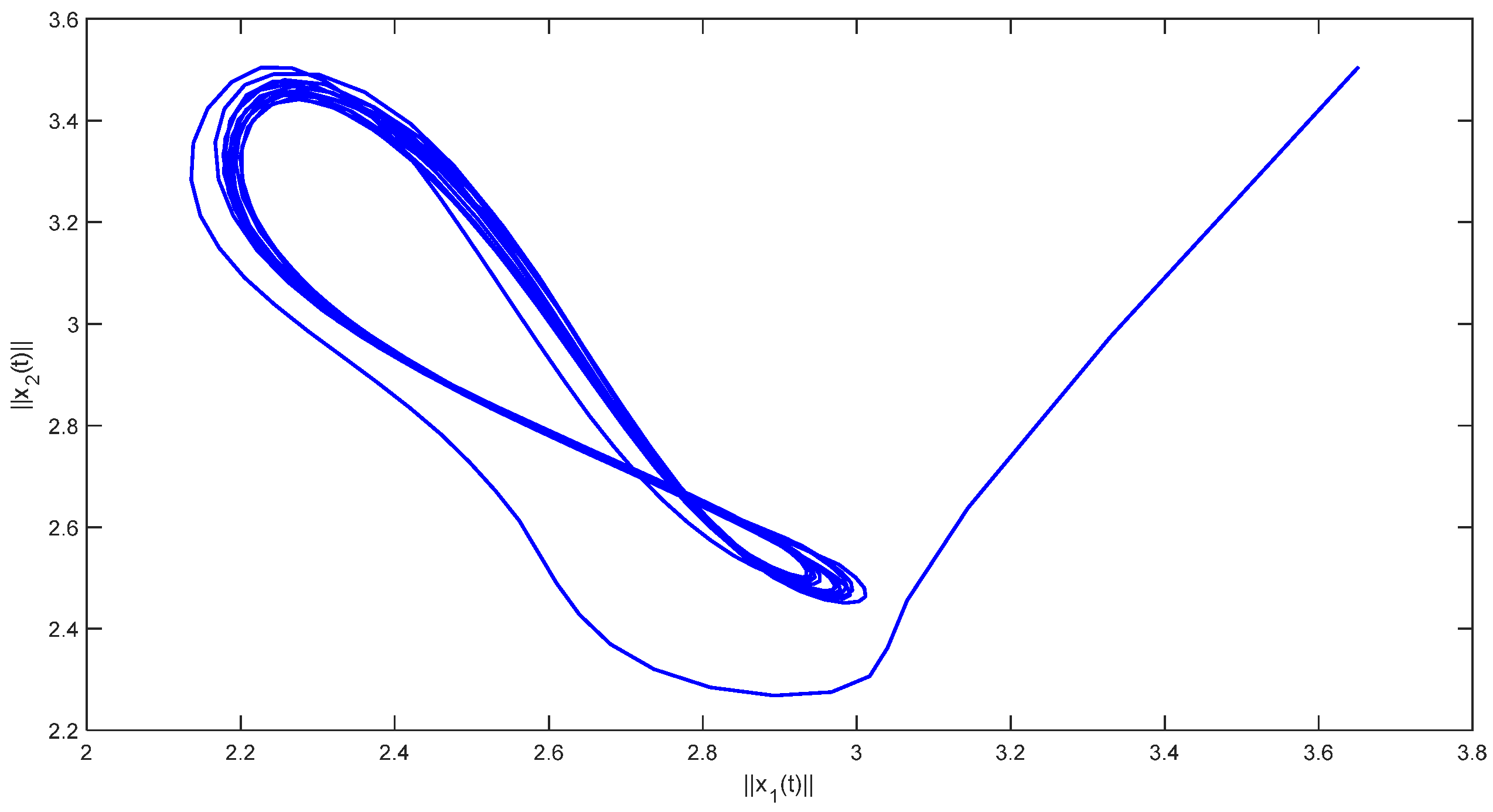
Figure 4.
Transient behaviors and synchronization errors of in system (35) and in system (36) with impulsive and stochastic disturbances.
Figure 4.
Transient behaviors and synchronization errors of in system (35) and in system (36) with impulsive and stochastic disturbances.
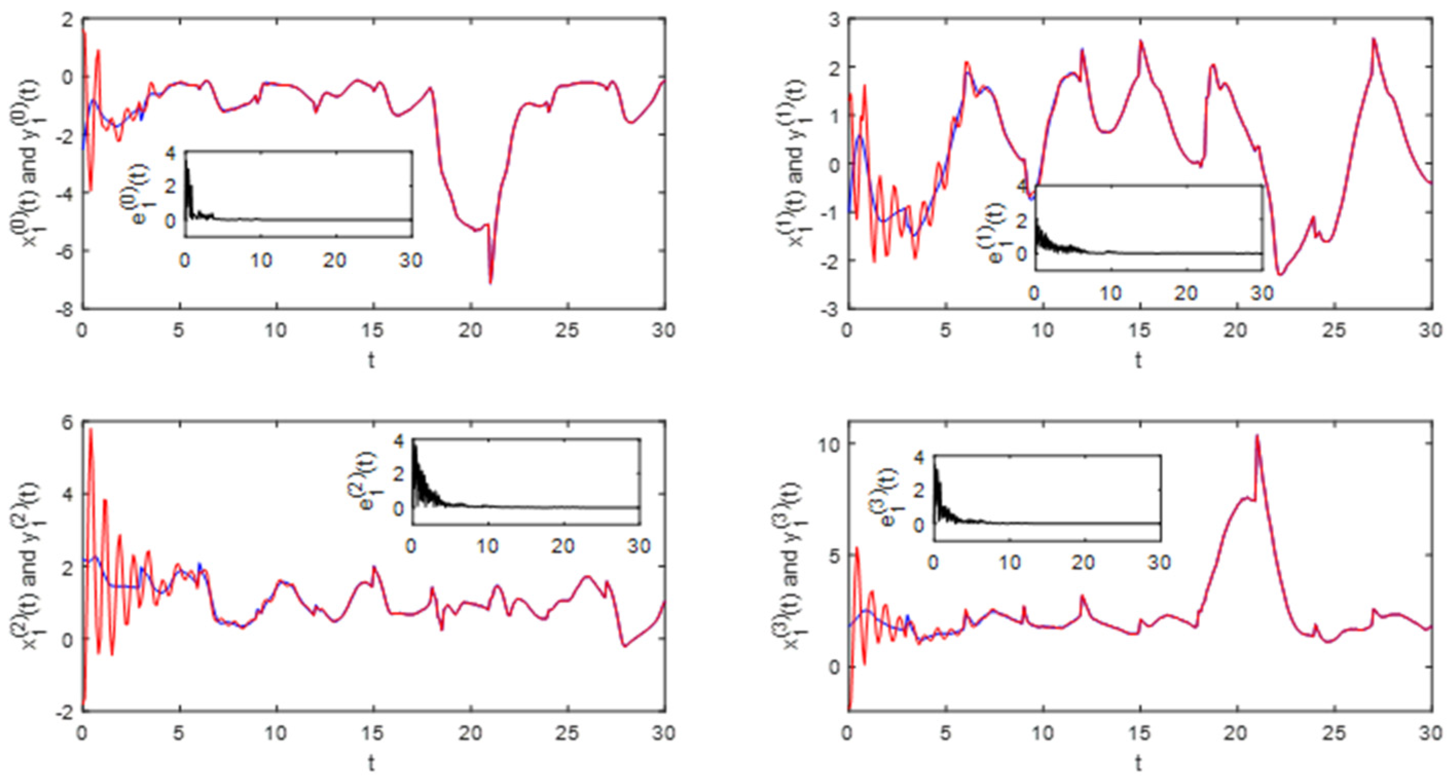
Figure 5.
Transient behaviors and synchronization errors of in system (35) and in system (36) with impulsive and stochastic disturbances.
Figure 5.
Transient behaviors and synchronization errors of in system (35) and in system (36) with impulsive and stochastic disturbances.
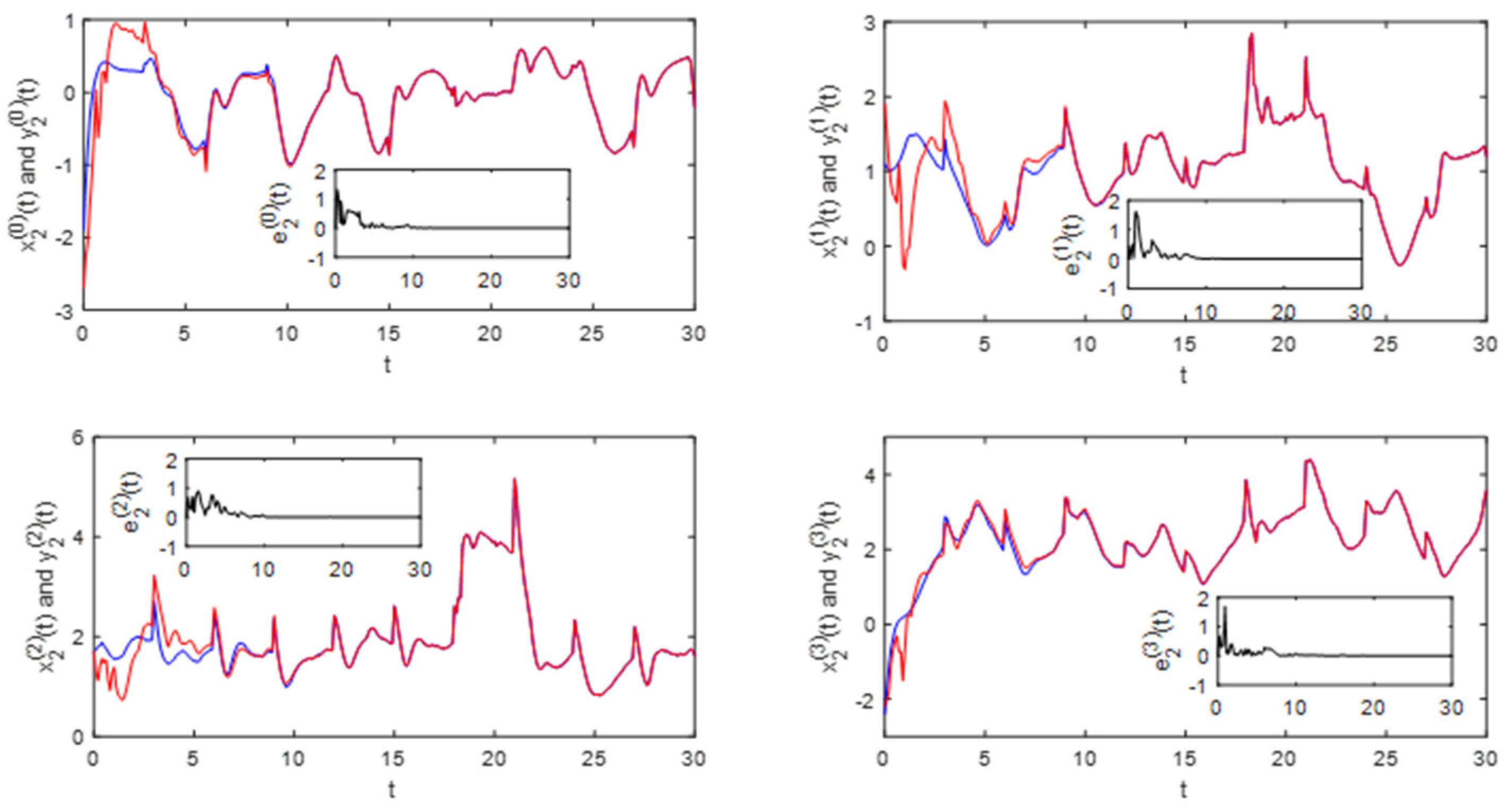
Figure 6.
Original color image of size 128 × 128 pixels.
Figure 7.
State curves of five neurons chosen randomly in the model (37) without impulsive and stochastic disturbances.
Figure 7.
State curves of five neurons chosen randomly in the model (37) without impulsive and stochastic disturbances.
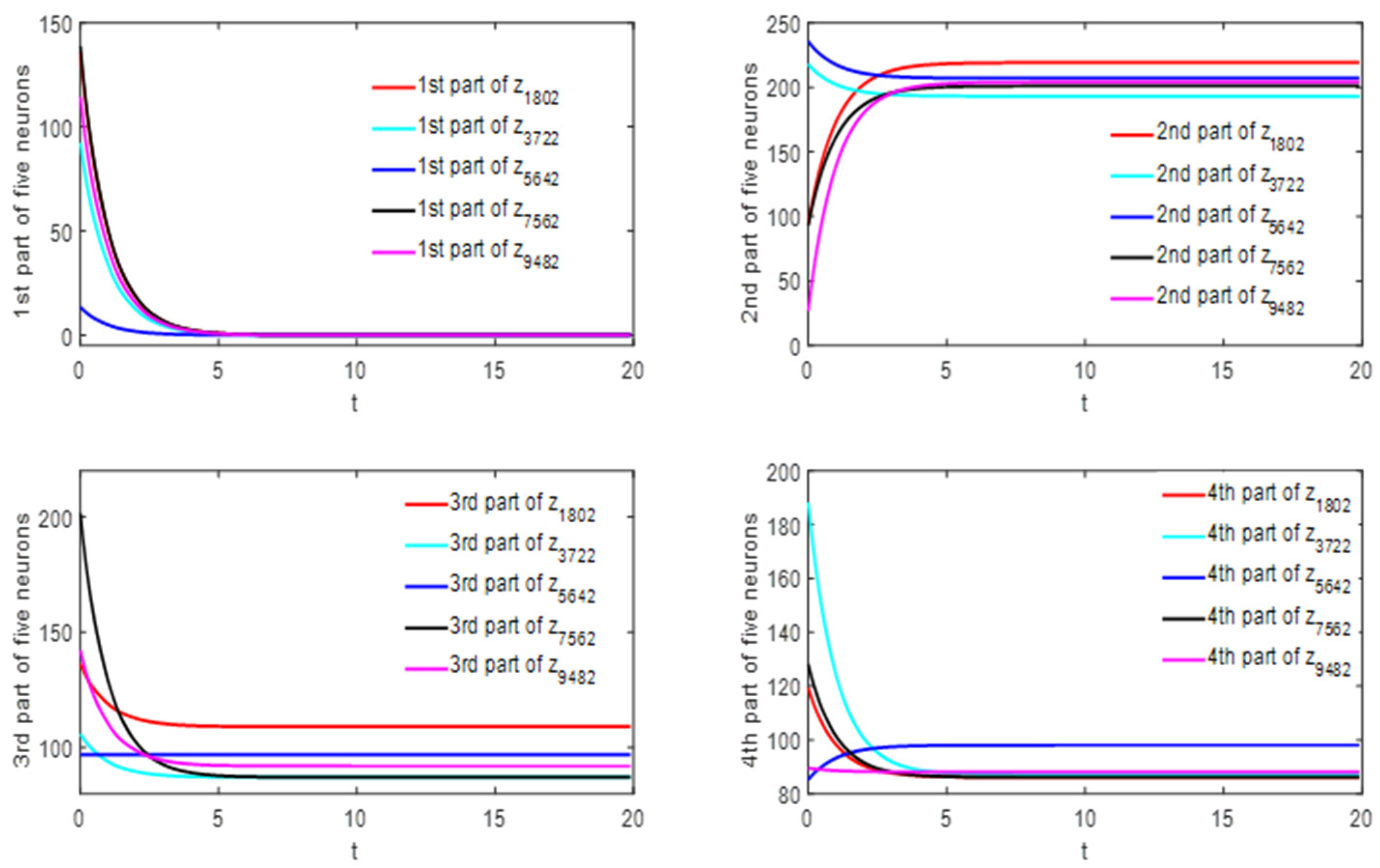
Figure 8.
State curves of five neurons chosen randomly in model (37) with impulses and stochastic disturbances in case 1.
Figure 8.
State curves of five neurons chosen randomly in model (37) with impulses and stochastic disturbances in case 1.
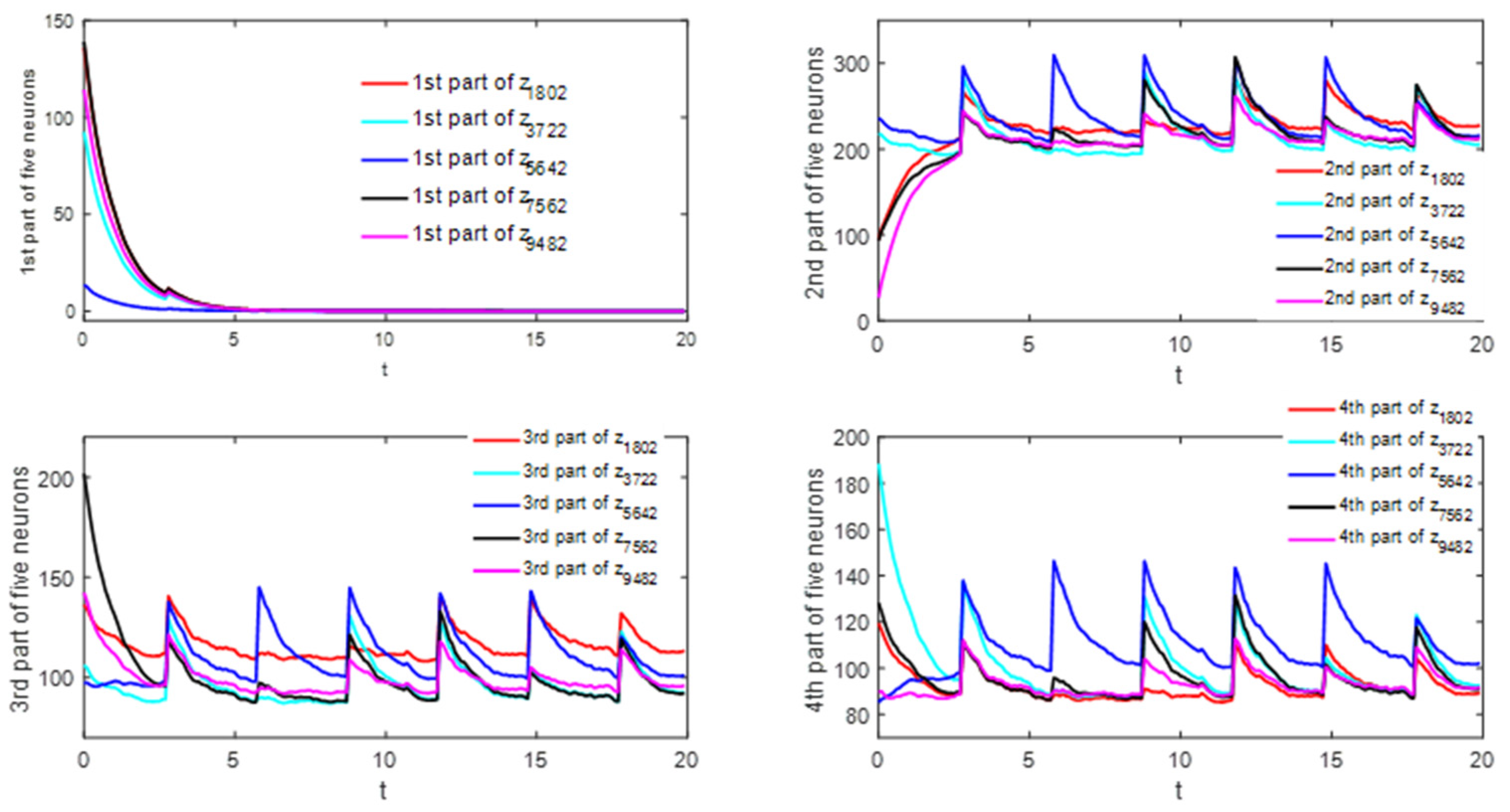
Figure 9.
Simulation results of retrieving the color image, where (a–f) are the retrieved image without disturbances, and (A–F) are the ones with disturbances under case 1.
Figure 9.
Simulation results of retrieving the color image, where (a–f) are the retrieved image without disturbances, and (A–F) are the ones with disturbances under case 1.

Figure 10.
State curves of five neurons chosen randomly in the model (37) with impulses and stochastic disturbances under case 2.
Figure 10.
State curves of five neurons chosen randomly in the model (37) with impulses and stochastic disturbances under case 2.
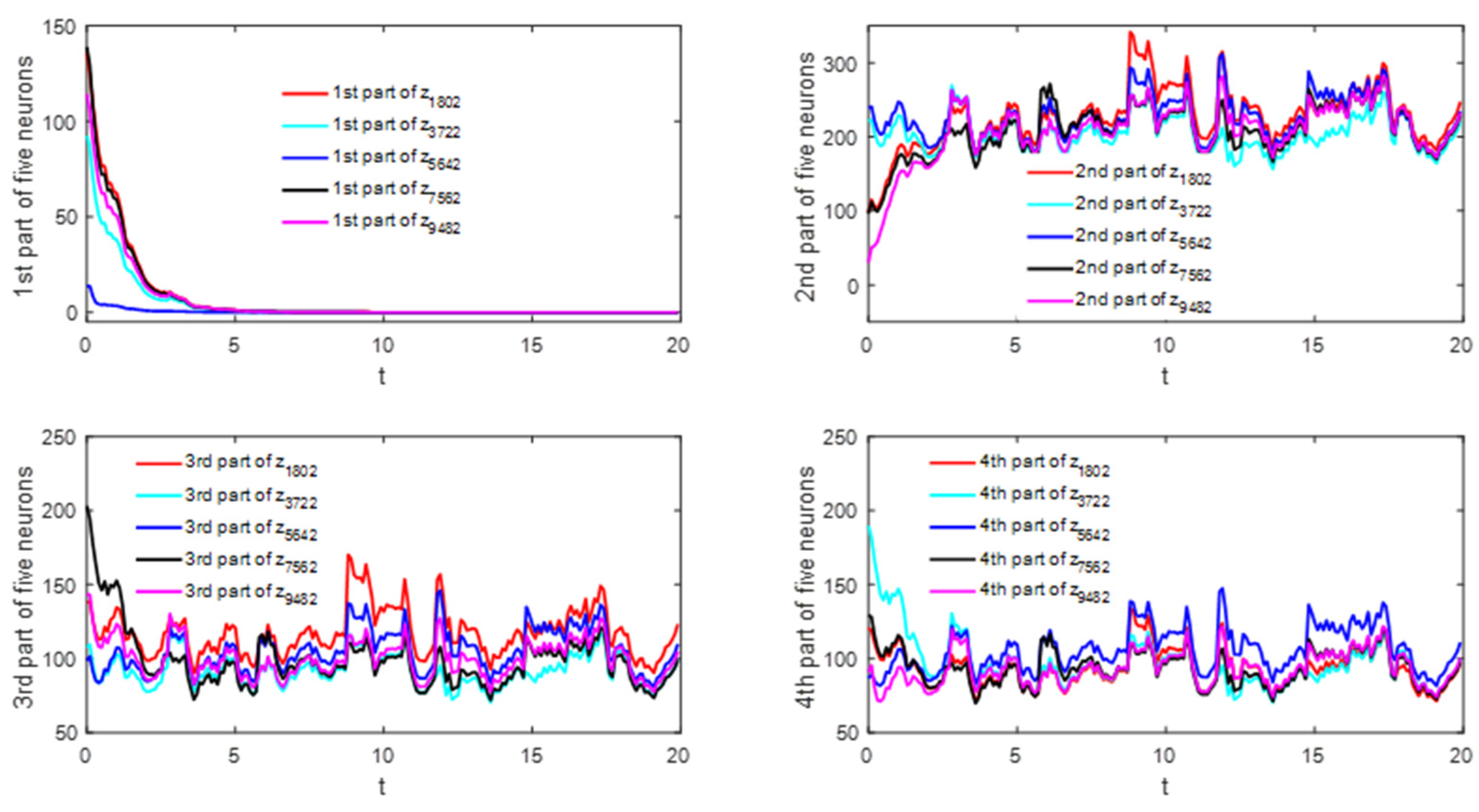
Figure 11.
Simulation results of retrieving the color image, where (a–f) are the retrieved image without disturbances, and (A–F) are the ones with disturbances under case 2.
Figure 11.
Simulation results of retrieving the color image, where (a–f) are the retrieved image without disturbances, and (A–F) are the ones with disturbances under case 2.


Table 1.
Necessary notations and means throughout the paper.
| Notations | Means | Notations | Means |
|---|---|---|---|
| real number domain | |||
| complex number domain | |||
| skew field of quaternions | |||
| natural number set | conjugate of defined as | ||
| set defined as | modulus of vector defined as | ||
| transpose of a vector or matrix | norm of defined as | ||
| imaginary unit | modulus of the matrix defined as | ||
| expectation function | complete probability space | ||
Table 2.
Literature summary of assumption for quaternion activation functions and study method.
| Types of Assumption | Decomposition Method | Non-Decomposition Method |
|---|---|---|
| Lipschitz condition | 9, 11, 13, 14, 19–21, 26 | 8, 12, 15–18, 22 |
| Boundedness | 10, 24 | none |
Table 3.
PSNR values of images in three cases.
| Three Cases | PSNR Value (dB) at Different Times (s) | |||||
|---|---|---|---|---|---|---|
| t = 0 | t = 1 | t = 3 | t = 5 | t = 10 | t = 20 | |
| case 0 (only impulsive disturbances) | 8.662 | 17.348 | 34.720 | 52.091 | 95.521 | 182.380 |
| case 1 (weak stochastic disturbances) | 8.662 | 17.266 | 16.880 | 31.904 | 24.492 | 31.141 |
| case 2 (strong stochastic disturbances) | 8.662 | 16.302 | 15.969 | 21.953 | 20.914 | 21.573 |
Disclaimer/Publisher’s Note: The statements, opinions and data contained in all publications are solely those of the individual author(s) and contributor(s) and not of MDPI and/or the editor(s). MDPI and/or the editor(s) disclaim responsibility for any injury to people or property resulting from any ideas, methods, instructions or products referred to in the content. |
© 2024 by the authors. Licensee MDPI, Basel, Switzerland. This article is an open access article distributed under the terms and conditions of the Creative Commons Attribution (CC BY) license (https://creativecommons.org/licenses/by/4.0/).
Share and Cite
MDPI and ACS Style
Yang, J.; Xu, X.; Xu, Q.; Yang, H.; Yu, M. Stability and Synchronization of Delayed Quaternion-Valued Neural Networks under Multi-Disturbances. Mathematics 2024, 12, 917. https://doi.org/10.3390/math12060917
AMA Style
Yang J, Xu X, Xu Q, Yang H, Yu M. Stability and Synchronization of Delayed Quaternion-Valued Neural Networks under Multi-Disturbances. Mathematics. 2024; 12(6):917. https://doi.org/10.3390/math12060917
Chicago/Turabian StyleYang, Jibin, Xiaohui Xu, Quan Xu, Haolin Yang, and Mengge Yu. 2024. "Stability and Synchronization of Delayed Quaternion-Valued Neural Networks under Multi-Disturbances" Mathematics 12, no. 6: 917. https://doi.org/10.3390/math12060917
Note that from the first issue of 2016, this journal uses article numbers instead of page numbers. See further details here.