Solid Isotropic Material with Penalization-Based Topology Optimization of Three-Dimensional Magnetic Circuits with Mechanical Constraints

Abstract

Topology optimization is currently enjoying renewed interest thanks to the recent development of 3D printing techniques, which offer the possibility of producing these new complex designs. One of the difficulties encountered in manufacturing topologically optimized magnetostatic structures is that they are not necessarily mechanically stable. In order to take this mechanical constraint into account, we have developed a SIMP-based topology optimization algorithm which relies on numerical simulations of both the mechanical deformation and the magnetostatic behavior of the structure. Two variants are described in this paper, respectively taking into account the compliance or the von Mises constraint. By comparing the designs obtained with those from magnetostatic optimization alone, our approach proves effective in obtaining efficient and robust designs.

1. Introduction

Topology optimization was first introduced to solve design problems in mechanics [1,2,3]. One of the most efficient approaches is based on the adjoint method [1,2,3] associated with SIMP penalization techniques [2,4]. From these works, topology optimization based on SIMP and adjoint approaches was extended to deal with design problems in electromagnetism such as magnetostatic issues [5,6] in order to design, for example, circuits of Hall effect thrusters [5,7] or electric machines [6,8]. Note that these design problems are mainly simplified by 2D approximations. Magnetostatic topology optimization based on the adjoint method associated with SIMP penalization techniques has been recently extended from 2D to 3D problems by some of this paper’s authors [9].

In all of these works, only one type of physics is considered in the optimization problem: either mechanics or magnetostatics. Thus, the designs obtained in magnetostatic problems are not always mechanically robust. They are sometimes not manufacturable and sometimes unable to withstand the mechanical stress experienced over their lifetime [10,11]. Note that a first study was recently conducted in [12] to develop a multiphysical topology optimization code to design electrical machines using 2D simplification.

Therefore, the purpose of this work is to address the 3D design problem of magnetostatic circuits, taking into account their mechanical robustness. Thus, this problem deals with two types of physics at the same time: mechanics and magnetostatics. The proposed approach combines the two physics through the use of a unique design variable. A continuous adjoint method associated with a SIMP penalization technique is developed to provide a topology optimization code which makes it possible to solve 3D design problems in magnetostatics while including mechanical considerations. In order to show the efficiency of this topology optimization code, a 3D design problem of a magnetic circuit is solved. Note that this simple magnetic circuit is similar to the circuit of Hall effect thrusters in [5,13].

In Section 2, we present the formulation of the 3D design problem we address in this work. This includes the definition of what variables and objective and constraint functions we will have to deal with. In Section 3, the SIMP penalization techniques as well as the continuous adjoint method are recalled, and the approach linking the mechanics and magneostatics is detailed. In Section 4, this topology optimization code dealing with two types of physics is validated through solving a 3D design example of a magnetic circuit. This design problem is detailed and the different results are discussed. Section 5 concludes the paper.

2. Formulation of the Coupled Mechanical and Magnetostatic Problem

In this paper, we focus on the optimization of a magnetic circuit similar to that of a Hall-effect thruster, as represented in Figure 1. It should be noted that the “toy” problem presented in this study is not intended to be fully representative of the real world, but rather is intended to allow a 3D magnetostatic problem to be considered without oversimplification.

This first section focuses on a comprehensive description of the physics involved in this study and is organized as follows: First, in Section 2.1, we describe the physics (PDE and objective function) behind the studied magnetic circuit. Second, in Section 2.2, we then present two mechanical constraints that are intended to yield manufacturable designs. Finally, in Section 2.3, we show how the two types of physics are coupled to define a unique topology optimization problem.

2.1. Magnetostatic Problem

The magnetic circuit consists of a copper coil enclosing a U-shaped iron structure surrounded by air. From a numerical point of view, the air is represented by a cube of finite size whose walls are sufficiently far from the structure so that they do not influence the simulation results. The full simulation domain is denoted by $\Omega \subset {\mathbb{R}}^3$, the coil by ${\Omega }_C\subset \Omega$, and the iron parts by ${\Omega }_I\subset \Omega$. The air regions are then given by ${\Omega }_A=\Omega \setminus ({\Omega }_C\cup {\Omega }_I)$; see Figure 2.

From the Maxwell–Ampere equation, the magnetic field $\mathbf{H}$ inside $\Omega$ is a solution to $\nabla \times \mathbf{H}=\mathbf{J}$, with $\mathbf{J}$ being a prescribed electric current which is equal to zero outside the coil, where $\mathbf{J}\left(\mathbf{x}\right)=\mathbf{0}$ for $\mathbf{x}\in \Omega \setminus {\Omega }_C$. In this work, the materials are assumed to be linear; hence, we use the following constitutive relation

$$\begin{array}{c}\hfill \mathbf{B}={\mu }_0{\mu }_r\left(\mathbf{H}+\mathbf{M}\right)\end{array}$$

(1)

between the magnetic flux density $\mathbf{B}$, magnetization $\mathbf{M}$, relative permeability ${\mu }_r$, and $\mathbf{H}$. Note that $\mathbf{M}=\mathbf{0}$ in this problem because there is no magnet. The permeability ${\mu }_r$ is equal to either ${\mu }_{\mathrm{air}}$ in the air and coil or ${\mu }_{\mathrm{iron}}$ inside the iron parts of the structure:

$$\begin{array}{c}\hfill {\mu }_r\left(\mathbf{x}\right)=\left\{\begin{array}{cc}{\mu }_{\mathrm{iron}}\hfill & \mathrm{if}\mathbf{x}\in {\Omega }_I\hfill \\ {\mu }_{\mathrm{air}}\hfill & \mathrm{elsewhere}\hfill \end{array}\right..\end{array}$$

(2)

From the Gauss law for magnetism $\nabla ·\mathbf{B}=\mathbf{0}$, there exists a vector potential $\mathbf{A}$ such that $\mathbf{B}=\nabla \times \mathbf{A}$ (unique up to a Gauge condition such as $\nabla ·\mathbf{A}=\mathbf{0}$). To summarize, $\mathbf{A}$ is solution to

$$\begin{array}{c}\hfill \left\{\begin{array}{ccc}\hfill -\nabla \times \left(\frac{1}{{\mu }_0{\mu }_r}\nabla \times \mathbf{A}\right)+\mathbf{J}=\mathbf{0}& \mathrm{in}& \Omega \hfill \\ \hfill \mathbf{n}\times \mathbf{A}=\mathbf{0}& \mathrm{on}& \partial \Omega \hfill \end{array}\right.\end{array}$$

(3)

in which a Dirichlet boundary condition on the borders $\partial \Omega$ of the domain is imposed to simulate the fact that the potential $\mathbf{A}$ is set to zero at infinity.

The aim of the magnetic circuit is to obtain a certain given field ${\mathbf{B}}_0$ within a target zone ${\Omega }_T$ located between the two “arms” of the structure. Indeed, in some applications, the aim is to impose a magnetic field in certain regions in order to improve the performance of the magnetic device. This is the case, for example, with the Hall-effect thruster shown in Figure 2, where the magnetic field traps electrons in certain regions and prevents them from striking and damaging the walls of the thruster. The problem presented in this article is a “toy” problem representative of this type of application, where a certain ${\mathbf{B}}_0$ field must be imposed in certain regions. To achieve this objective, we will optimize the distribution of matter (iron and air) within a region ${\Omega }_V\subset \Omega$ (the index V refers to the variable nature of this region). To accomplish this, we define a distribution $\varrho :{\Omega }_V\to \{0,1\}$ equal to either one or zero at each position $\mathbf{x}\in {\Omega }_V$ such that

$$\begin{array}{c}\hfill {\mu }_r\left(\mathbf{x}\right)={\mu }_{\mathrm{air}}+({\mu }_{\mathrm{iron}}-{\mu }_{\mathrm{air}})\varrho \left(\mathbf{x}\right).\end{array}$$

(4)

We then search for the optimal distribution ${\varrho }^{\ast }$ (which define an optimal shape ${\Omega }_{V,I,\mathrm{opt}}=\{\mathbf{x},{\varrho }^{\ast }\left(\mathbf{x}\right)=1\}$ for the iron part inside the variable region) which minimizes the error between the actual field $\mathbf{B}\left(\varrho \right)=\nabla \times \mathbf{A}\left(\varrho \right)$ solution of Equation (3) using Equation (4) (note that to simplify the notations, the dependency on $\varrho$ is not always specified hereafter) and the target one ${\mathbf{B}}_0$:

$$\begin{array}{c}\hfill {\varrho }^{\ast }=\underset{\varrho }{arg\; min}{F}_1\left(\varrho \right)\mathrm{where}{F}_1\left(\varrho \right)={\int }_{{\Omega }_T}{\parallel \mathbf{B}\left(\varrho \right)-{\mathbf{B}}_0\parallel }^2\mathrm{d}\mathbf{x}.\end{array}$$

(5)

2.2. Mechanical Problem

The main objective of introducing mechanics in the optimization problem is to design magnetic parts that are mechanically robust. This is achieved by taking into account the mechanical loads that the parts will be subjected to during their future use. The load considered in this article is an arbitrary load that the part will encounter over its life time. Moreover, the mechanical considerations will tackle the problem of shapes that are mechanically unstable, in particular regions floating in the air, as seen in Section 4. We therefore present here two measures of the mechanical strength of the optimized structure based on simulations of the mechanical deformations caused by an arbitrary load $\mathbf{g}$ applied to both end ${\Gamma }_L$ of the structure arms assuming that the optimized shape is clamped on the non-variable iron parts ${\Gamma }_I$; see Figure 3.

According to the principle of conservation of linear momentum, when no forces are applied to the structure, the stress tensor $\overline{\overline{\sigma }}$ inside the optimized region verifies $\nabla ·\overline{\overline{\sigma }}=\mathbf{0}$. Under Hooke’s law, the displacement vector $\mathbf{u}$ is related to $\overline{\overline{\sigma }}$ through

$$\begin{array}{c}\hfill \overline{\overline{\sigma }}\left(\mathbf{u}\right)=2\mu \overline{\overline{e}}\left(\mathbf{u}\right)+\lambda \mathrm{tr}\left(\overline{\overline{e}}\left(\mathbf{u}\right)\right){\mathrm{I}}_3=A\overline{\overline{e}}\left(\mathbf{u}\right)\end{array}$$

(6)

where $\lambda$ and $\mu$ are the Lamé coefficients, and can be expressed in terms of the Young’s modulus E and the Poisson ratio $\nu$ by

$$\lambda =\frac{\nu E}{(1+\nu )(1-2\nu )}\mathrm{and}\mu =\frac{E}{2(1+\nu )}$$

while A is a fourth-order elasticity tensor containing these mechanical properties. In the context of small perturbations, the deformation tensor $\overline{\overline{e}}\left(\mathbf{u}\right)$ is also given by $\overline{\overline{e}}\left(\mathbf{u}\right)=(\nabla \mathbf{u}+\nabla {\mathbf{u}}^T)/2$. We denote by $E_{\mathrm{iron}}$ and $\nu =0.3$ the mechanical properties inside the iron material. As is common in topology optimization of mechanical structures, we consider air to be a very soft material with a small Young’s modulus $E_{\mathrm{air}}\simeq 0$ and $\nu =0.3$. Using the distribution of matter $\varrho :{\Omega }_V\to \{0,1\}$ inside the variable region again, we then have the following for $\mathbf{x}\in {\Omega }_V$:

$$\begin{array}{c}\hfill E\left(\mathbf{x}\right)=E_{\mathrm{air}}+(E_{\mathrm{iron}}-E_{\mathrm{air}})\varrho \left(\mathbf{x}\right).\end{array}$$

(7)

This makes it possible to define the displacement field $\mathbf{u}\left(\varrho \right)$ as the only solution of the following problem:

$$\begin{array}{c}\hfill \left\{\begin{array}{ccc}\hfill -\nabla ·\left[A\left(\varrho \right)\overline{\overline{e}}\left(\mathbf{u}\left(\varrho \right)\right)\right]=\mathbf{0}& \mathrm{in}& {\Omega }_V\hfill \\ \hfill \mathbf{u}\left(\varrho \right)=\mathbf{0}& \mathrm{on}& {\Gamma }_I\hfill \\ \hfill A\left(\varrho \right)\overline{\overline{e}}\left(\mathbf{u}\left(\varrho \right)\right)\mathbf{n}=\mathbf{g}& \mathrm{on}& {\Gamma }_L\hfill \\ \hfill A\left(\varrho \right)\overline{\overline{e}}\left(\mathbf{u}\left(\varrho \right)\right)\mathbf{n}=\mathbf{0}& \mathrm{on}& \partial {\Omega }_V\setminus \left({\Gamma }_I\cup {\Gamma }_L\right)\hfill \end{array}\right..\end{array}$$

(8)

We now define two figures of merit that will be taken into account in order to ensure the mechanical strength of the topologically optimized design:

• The first criterion to ensure robustness of the structure is to maximize its rigidity, which is equivalent to minimizing its compliance. In other words, we want a distribution $\varrho$ which minimizes

  $$\begin{array}{cc}\hfill F_2\left(\varrho \right)& ={\int }_{{\Gamma }_L}\mathbf{g}·\mathbf{u}\left(\varrho \right)\mathrm{d}\mathbf{s}.\hfill \end{array}$$

  (9)
• The second criterion is based on the von Mises stress ${\sigma }_{VM}$ expressed in terms of the components of the stress tensor $\overline{\overline{\sigma }}$ as follows:

  $$\begin{array}{c}\hfill {\sigma }_{VM}={\left({\sigma }_{xx}^2+{\sigma }_{yy}^2+{\sigma }_{zz}^2-{\sigma }_{xx}{\sigma }_{yy}-{\sigma }_{yy}{\sigma }_{zz}-{\sigma }_{zz}{\sigma }_{xx}+3{\sigma }_{xy}^2+3{\sigma }_{yz}^2+3{\sigma }_{zx}^2\right)}^{\frac{1}{2}}.\end{array}$$

  (10)
  The aim here is to minimize the maximal value taken by ${\sigma }_{VM}$ inside the optimized iron shape where $\varrho \left(\mathbf{x}\right)=1$, i.e.,

  $$\begin{array}{c}\hfill \parallel \varrho {\sigma }_{VM}{\parallel }_{\infty }=\underset{\mathbf{x}\in {\Omega }_V}{max}\varrho \left(\mathbf{x}\right){\sigma }_{VM}\left(\mathbf{x}\right).\end{array}$$
  Note that here the stress measure is defined by the relaxed stress $\varrho {\sigma }_{VM}$ instead of ${\sigma }_{VM}$ in order to ensure that the stress measure is zero in the air region where $\varrho \left(\mathbf{x}\right)=0$ [14]. As the use of an infinite norm raises difficulties for the optimization method, we will instead use the following Kreisselmeier–Steinhauser (KS) function, $F_{3,p}\left(\varrho \right)\simeq {\parallel \varrho {\sigma }_{VM}(\varrho ,\mathbf{u}\left(\varrho \right))\parallel }_{\infty }$, which is valid for large values of p:

  $$\begin{array}{cc}\hfill F_{3,p}\left(\varrho \right)& ={\left({\int }_{{\Omega }_V}{\left[\varrho {\sigma }_{VM}(1,\mathbf{u}\left(\varrho \right))\right]}^p\mathrm{d}\mathbf{x}\right)}^{\frac{1}{p}}.\hfill \end{array}$$

  (11)

2.3. Link between the Two Types of Physics

We have seen in the previous sections that the material distribution $\varrho \left(\mathbf{x}\right)$ is responsible for both the magnetic ${\mu }_r\left(\mathbf{x}\right)$ (with Equation (4)) and mechanical $E\left(\mathbf{x}\right)$ (with Equation (7)) properties by defining iron (resp., air) regions where $\varrho \left(\mathbf{x}\right)=1$ (resp., $\varrho \left(\mathbf{x}\right)=0$). We can thus define a coupled optimization problem in which an optimal distribution $\varrho$ is sought such that it simultaneously minimizes the error between $\mathbf{B}$ and ${\mathbf{B}}_0$ (Equation (5)) while simultaneously minimizing one of the two mechanical criteria of Equation (9) or Equation (11).

To achieve this, we will first optimize the magnetic circuit alone without any mechanical constraint in order to find an unstable optimal distribution ${\varrho }_0^{\ast }$ which minimizes $F_1$. In a second step, we will consider the following problem, which consists of minimizing one of the two mechanical criteria $F_2$ or $F_3$ under the constraint of preserving good magnetic performance close to those of ${\varrho }_0^{\ast }$:

$$\left(\mathcal{P}\right)\left\{\begin{array}{cc}\underset{\varrho }{min}\hfill & F_2\left(\varrho \right)\left(\mathrm{or}{F}_{3,p}\left(\varrho \right)\right)\hfill \\ u.c.\hfill & F_1\left(\varrho \right)\le F_1\left({\varrho }_0^{\ast }\right)+ϵ\hfill \end{array}\right.$$

(12)

where $ϵ>0$ is a small value.

3. A SIMP-Based Optimization Problem

Solving problem $\left(\mathcal{P}\right)$ of Equation (12), in which $\varrho :{\Omega }_V\to \{0,1\}$ is a distribution that can only take the values 0 or 1, is a numerically difficult task. Instead, we can relax the latter constraint and look for a material distribution $\rho :{\Omega }_V\to [0,1]$ that accepts any intermediate value between 0 and 1. Thus, a continuous optimization problem is obtained (for which an efficient gradient-based method can be used) rather than a discrete one. To achieve a true material distribution with only iron ($\rho \left(\mathbf{x}\right)=1$) or air ($\rho \left(\mathbf{x}\right)=0$) at the end of the optimization process, it is necessary to penalize intermediate values of $\rho$ during the gradient descent. This is the principle behind the well-known solid isotropric material with penalization (SIMP) method [2,4,9].

In the next Section 3.1, the main method to deal with the penalization issue is recalled. In Section 3.2, we then show how computing the gradients of the functions $F_1$, $F_2$, and $F_3$ presented in Section 2 is possible using adjoint states obtained via the Céa method introduced in [15]. These gradients are then used in Section 3.3 to implement an optimization algorithm which can be used to solve problem $\left(\mathcal{P}\right)$.

3.1. Penalization with Material Density Method

As previously explained, the constraint on the values taken by $\rho \left(\mathbf{x}\right)$ has been relaxed to the whole $[0,1]$ interval to simplify the optimization process. However, to prevent the appearance of intermediate values in the optimal distribution ${\rho }^{\ast }\left(\mathbf{x}\right)$, the SIMP method suggests penalizing the values of $\rho$, which are used in the definition of the material properties in the following way:

$$\begin{array}{cc}\hfill {\mu }_r\left(\mathbf{x}\right)& ={\mu }_{\mathrm{air}}+({\mu }_{\mathrm{iron}}-{\mu }_{\mathrm{air}})g\left(\rho \left(\mathbf{x}\right)\right)\hfill \\ \hfill E\left(\mathbf{x}\right)& =E_{\mathrm{air}}+(E_{\mathrm{iron}}-E_{\mathrm{air}})g\left(\rho \left(\mathbf{x}\right)\right)\hfill \end{array}$$

with $g:[0,1]\to [0,1]$ being a non-decreasing interpolation function verifying $g\left(0\right)=0$ and $g\left(1\right)=1$. In the literature, there are several choices of interpolation functions g that influence the final result of topology optimization [2,4,16]. In this work, we use the polynomial interpolation function for its simplicity [4], which is defined by

$$\begin{array}{c}\hfill g\left(x\right)=x^n\mathrm{and}{g}^{\prime }\left(x\right)=n{x}^{n-1}\end{array}$$

(13)

where $n>0$ is a penalty parameter that will be incremented during the optimization process. As n goes up, the optimal solution tends to become discrete, with values closer to either 0 or 1. It is worth noting that this interpolation function is not symmetrical, and hence it favors materials with low values of $\rho$ (i.e., air).

Remark 1.

In the definition of the objective function $F_{3,p}$ described in Equation (11), we consider the von Mises stress inside the iron structure. Now that intermediate materials can be present in the optimized design, we need to relax the definition of $F_{3,p}$. Following [17], Equation (11) is modified into:

$$\begin{array}{cc}\hfill {\widehat{F}}_{3,p}\left(\rho \right)& ={\left({\int }_{{\Omega }_V}{\left[{\rho }^m{\sigma }_{VM}(1,\mathit{u}\left(\rho \right))\right]}^p\mathit{d}\mathsf{x}\right)}^{\frac{1}{p}}\hfill \end{array}$$

(14)

with $m>0$ ($m=1/2$ in the numerical examples of Section 4).

3.2. Sensitivity Analysis

In this section, the sensitivities of the three objective functions $F_1$, $F_2$ and ${\widehat{F}}_{3,p}$ with respect to the design variable $\rho$ are provided. Regarding the magnetostatic problem, the following proposition is verified:

Proposition 1

(Sensitivity of $F_1$ with respect to $\rho$). The expression of the sensitivity of $F_1$ with respect to the design variable ρ is:

$$〈F_1^{\prime }\left(\rho \right),\tilde{\rho }〉={\int }_{{\Omega }_V}\frac{({\mu }_{\mathit{iron}}-{\mu }_{\mathit{air}})g^{\prime }\left(\rho \right)\tilde{\rho }}{{({\mu }_{\mathit{air}}+({\mu }_{\mathit{iron}}-{\mu }_{\mathit{air}})g\left(\rho \right))}^2}{\mathit{B}}_{\mathit{adj}}·\mathit{B}\mathit{d}\mathsf{x}$$

(15)

in which $\mathit{B}$ is given by the direct problem of Equation (3) and ${\mathit{B}}_{\mathit{adj}}=\nabla \times {\mathit{A}}_{\mathit{adj}}$ is an “adjoint” field solution of

$$\begin{array}{c}\hfill \left\{\begin{array}{ccc}\hfill -\nabla \times \left(\frac{1}{{\mu }_0{\mu }_r}\nabla \times {\mathit{A}}_{\mathit{adj}}-{\mathit{M}}_{\mathit{adj}}\right)=\mathbf{0}& \mathit{in}& \Omega \hfill \\ \hfill \mathit{n}\times {\mathit{A}}_{\mathit{adj}}=\mathbf{0}& \mathit{on}& \partial \Omega \hfill \end{array}\right.\end{array}$$

(16)

where ${\mathit{M}}_{\mathit{adj}}$ is a magnetization source which is non-zero inside ${\Omega }_T$ and defined as follows:

$$\begin{array}{c}\hfill {\mathit{M}}_{\mathit{adj}}=\frac{2}{{\mu }_0}\left(\mathit{B}-{\mathit{B}}_0\right){\mathbb{1}}_{{\Omega }_T}.\end{array}$$

We already proved this proposition in [9]. Similarly, for the first mechanical constraint $F_2$, we have:

Proposition 2

(Sensitivity of $F_2$ with respect to $\rho$). The expression of the sensitivity of $F_2$ with respect to the design variable ρ in a direction $\tilde{\rho }$ is given by

$$〈F_2^{\prime }\left(\rho \right),\tilde{\rho }〉=-{\int }_{{\Omega }_V}{A}^{{\ast }^{\prime }}\left(\rho \right)\overline{\overline{e}}\left(\mathit{u}\right):\overline{\overline{e}}\left(\mathit{u}\right)\tilde{\rho }d\mathsf{x}$$

(17)

where $A^{\ast }\left(\rho \right)=\left[\frac{E_{\mathit{air}}}{E_{\mathit{iron}}}+(1-\frac{E_{\mathit{air}}}{E_{\mathit{iron}}})g\left(\rho \right)\right]A\left(1\right)$.

In this case, the problem is said to be auto-adjoint (the adjoint is the same as the direct solution $\mathbf{u}$). The proof is detailed in Appendix A. And finally, for $F_3$, we find the following proposition holds:

Proposition 3

(Sensitivity of ${\widehat{F}}_{3,p}$ with respect to $\rho$). The expression of the sensitivity of ${\widehat{F}}_{3,p}$ with respect to the variable design ρ in a direction $\tilde{\rho }$ is given by

$$\begin{array}{c}〈{\widehat{F}}_{3,p}^{\prime }\left(\rho \right),\tilde{\rho }〉={\int }_{{\Omega }_V}{A}^{{\ast }^{\prime }}\left(\rho \right)\overline{\overline{e}}\left(\mathit{u}\right):\overline{\overline{e}}\left(\mathit{p}\right)\tilde{\rho }\mathit{d}\mathsf{x}\hfill \\ \hfill \hspace{1em}\hspace{1em}\hspace{1em}\hspace{1em}\hspace{1em}\hspace{1em}\hspace{1em}+{\left({\int }_{{\Omega }_V}{\rho }^{mp}{\sigma }_{VM}{(1,\mathit{u})}^p\mathit{d}\mathsf{x}\right)}^{\frac{1}{p}-1}{\int }_{{\Omega }_V}m{\sigma }_{VM}^p(1,\mathit{u}){\rho }^{mp-1}\tilde{\rho }\mathit{d}\mathsf{x}\end{array}$$

(18)

where $\mathit{p}$ is the adjoint state, a solution for all $\mathit{v}\in V$, where

$$\begin{array}{c}\hfill V={\left(H_0^1\left({\Omega }_V\right)\right)}^3=\left\{\mathit{v}\in {\left(H^1\left({\Omega }_V\right)\right)}^3,\mathit{v}=\mathbf{0}\mathit{on}{\Gamma }_I\right\}\end{array}$$

(19)

of the following variational formulation:

$$\begin{array}{c}{\left({\int }_{{\Omega }_V}{\rho }^{mp}{\sigma }_{VM}^p(1,\mathit{u})\mathit{d}\mathsf{x}\right)}^{\frac{1}{p}-1}{\int }_{{\Omega }_V}{\rho }^{mp}{\sigma }_{VM}^{p-1}(1,\mathit{u}){\frac{\partial {\sigma }_{VM}}{\partial \overrightarrow{\sigma }}}^T\overrightarrow{\sigma }\left(\mathit{v}\right)\mathit{d}\mathsf{x}\hfill \\ \hfill \hspace{1em}\hspace{1em}\hspace{1em}\hspace{1em}\hspace{1em}\hspace{1em}\hspace{1em}\hspace{1em}\hspace{1em}\hspace{1em}\hspace{1em}\hspace{1em}\hspace{1em}\hspace{1em}\hspace{1em}\hspace{1em}\hspace{1em}\hspace{1em}+{\int }_{{\Omega }_V}{A}^{\ast }\left(\rho \right)\overline{\overline{e}}\left(\mathit{v}\right):\overline{\overline{e}}\left(\mathit{p}\right)\mathit{d}\mathsf{x}=0\end{array}$$

(20)

where $\overrightarrow{\sigma }$ is the Voigt notation for constraints $\overline{\overline{\sigma }}$ defined by

$$\overrightarrow{\sigma }={({\sigma }_{xx},{\sigma }_{yy},{\sigma }_{zz},{\sigma }_{xy},{\sigma }_{yz},{\sigma }_{zx})}^T$$

and

$$\frac{\partial {\sigma }_{VM}}{\partial \overrightarrow{\sigma }}=\left(\begin{array}{c}\frac{\partial {\sigma }_{VM}}{\partial {\sigma }_{xx}}\\ \frac{\partial {\sigma }_{VM}}{\partial {\sigma }_{yy}}\\ \frac{\partial {\sigma }_{VM}}{\partial {\sigma }_{zz}}\\ \frac{\partial {\sigma }_{VM}}{\partial {\sigma }_{xy}}\\ \frac{\partial {\sigma }_{VM}}{\partial {\sigma }_{yz}}\\ \frac{\partial {\sigma }_{VM}}{\partial {\sigma }_{zx}}\end{array}\right)=\left(\begin{array}{c}\frac{1}{2{\sigma }_{VM}}(2{\sigma }_{xx}-{\sigma }_{yy}-{\sigma }_{zz})\\ \frac{1}{2{\sigma }_{VM}}(2{\sigma }_{yy}-{\sigma }_{xx}-{\sigma }_{zz})\\ \frac{1}{2{\sigma }_{VM}}(2{\sigma }_{zz}-{\sigma }_{xx}-{\sigma }_{yy})\\ \frac{3}{{\sigma }_{VM}}\left({\sigma }_{xy}\right)\\ \frac{3}{{\sigma }_{VM}}\left({\sigma }_{yz}\right)\\ \frac{3}{{\sigma }_{VM}}\left({\sigma }_{zx}\right)\end{array}\right).$$

(21)

This proposition is also proven in Appendix A. Note that the proof of these three propositions are all based on the following four steps (which are theoretically based on [1,2] and detailed in either [9] or Appendix A):

• Definition of a constrained optimization problem in which $J(\rho ,\mathbf{w})=F\left(\rho \right)$ is given by either $F_1,$ $F_2$, or ${\widehat{F}}_{3,p}$ and $\mathbf{w}$ is either the magnetic potential $\mathbf{A}$ or the displacement $\mathbf{u}$ (solution of the PDE $L_{\rho }\left(\mathbf{w}\right)=f$):

  $$\left\{\begin{array}{cc}\underset{\rho ,\mathbf{w}}{min}\hfill & J(\rho ,\mathbf{w})\hfill \\ u.c.\hfill & L_{\rho }\left(\mathbf{w}\right)=f\mathrm{and}\rho \in L^{\infty }({\Omega }_V,[0,1])\hfill \end{array}\right..$$
• Introduction of a Lagrange multiplier $\mathit{\lambda }$ associated with the constraint $L_{\rho }\left(\mathbf{w}\right)=f$ to obtain a Lagrangian function $\mathcal{L}(\rho ,\mathbf{w},\mathit{\lambda })$.
• Determination of the adjoint state ${\mathbf{w}}_{\mathrm{adj}}$ solution of an adjoint equation $L_{\rho }\left({\mathbf{w}}_{\mathrm{adj}}\right)=f_{\mathrm{adj}}$ from the Karush–Khun–Tucker theorem (partial derivatives of the Lagrangian with regard to $\mathbf{w}$ and $\mathit{\lambda }$ equal to zero).
• Computation of $〈F^{\prime }\left(\rho \right),\tilde{\rho }〉=〈\frac{\partial \mathcal{L}}{\partial \rho }(\rho ,\mathbf{w},{\mathbf{w}}_{\mathrm{adj}}),\tilde{\rho }〉$ yields the sensitivity of the objective function with respect to the design variable $\rho$; derivation of the Lagrangian with regard to $\rho$; and evaluation using the solutions $\mathbf{w}$ and ${\mathbf{w}}_{\mathrm{adj}}$ of the direct and adjoint problems.

Now that the derivatives of the three objective functions have been derived, we can define in the next section the general algorithm that will be used to solve problem $\left(\mathcal{P}\right)$.

3.3. Optimization Algorithm

From a numerical point of view, the distribution $\rho :{\Omega }_V\to [0,1]$ will need to be discretized. Since the magnetostatic and mechanical PDEs of Equations (3) and (8) are solved using the Finite Element Method (FEM), the variable domain ${\Omega }_V$ is already discretized into N open sets (tetrahedrons) $T_i$ such that ${\overline{\Omega }}_V={\cup }_{i=1}^N{\overline{T}}_i$ and $T_i\cap T_j=\varnothing$ for all $i\ne j$. We then naturally discretize $\rho$ into a vector $\mathit{\rho }={({\rho }_1,\dots ,{\rho }_N)}^T$ of N values such that for all $\mathbf{x}\in {\Omega }_V$:

$$\begin{array}{c}\hfill \rho \left(\mathbf{x}\right)=\sum _{i=1}^N{\rho }_i{\mathbb{1}}_{T_i}\left(\mathbf{x}\right).\end{array}$$

(22)

Using this discretization, the sensitivity of any objective function F with regard to ${\rho }_i\in \mathbb{R}$ in the direction ${\tilde{\rho }}_i$ (to simplify, we use the same notation for F depending on either $\rho$ or $\mathit{\rho }$) is given by:

$$\begin{array}{c}\hfill 〈F^{\prime }\left(\mathit{\rho }\right),{\tilde{\rho }}_i〉=〈F^{\prime }\left(\rho \right),{\mathbb{1}}_{T_i}〉{\tilde{\rho }}_i\end{array}$$

where each term $〈F^{\prime }\left(\rho \right),{\mathbb{1}}_{T_i}〉$ is an integral on the set $T_i$. In order to solve problem $\left(\mathcal{P}\right)$, we will use the MMA gradient-based algorithm [18], which requires the following ingredients:

• The mechanical objective function (Equations (9) and (14)) and its associated gradient with respect to each ${\rho }_i$ (see Equations (17), (18) and (22)).
• The magnetostatic constraint (Equation (5)) and its associated gradient with respect to each ${\rho }_i$ (see Equations (15) and (22)).
• The constraints on $\mathit{\rho }$ which are only the lower and upper bounds of the material density: $\mathit{\rho }\in {[0,1]}^N$.

Like any local optimization algorithm based on gradient descent, this optimization module starts from a starting point denoted by ${\mathit{\rho }}^{\left[0\right]}$, builds a sequence of points ${\mathit{\rho }}^{\left[k\right]}$, and ends at ${\mathit{\rho }}^{\ast }$. During the process of optimization, the penalty parameter n used in Equation (13) is increased when the objective function stagnates. This makes it possible to converge slowly but strongly to efficient design solutions [4,19,20].

Remark 2.

Using this classical method, the final solution generally has a checkerboard patterns [3]. In order to make the solution more manufacturable, a regularization method must be added. Thus, in this work, a density filtering method is used. It consists of modifying the value of ρ used inside each tetrahedron into a weighted sum of its current value and the values of its neighboring tetrahedrons. The implementation details and associated modified gradient follow the procedure described in [3].

4. Numerical Examples

The aim of this section is to validate our methodology on a U-shaped magnetic circuit. We begin by giving all the geometrical parameters of the structure in Section 4.1. We then move on to the solution of the magnetostatic problem alone in Section 4.2. Finally in Section 4.3 and Section 4.4 we solve the hybrid problem $\left(\mathcal{P}\right)$ and discuss the results in detail.

4.1. Design Problem

We consider here a simple magnetic circuit, shown in the right of Figure 1, with one coil and two distinct variable zones which can be either air or a ferromagnetic material (iron). For this magnetic circuit, the design variable is the material distribution $\rho$ which varies between its maximal value of 1 (corresponding to ferromagnetic material: ${\mu }_{\mathrm{iron}}=3000$ and $E_{\mathrm{iron}}=0.21$ GPa) and minimal value of 0 (corresponding to air: ${\mu }_{\mathrm{air}}=1$ and $E_{\mathrm{air}}={10}^{-10}{E}_{\mathrm{iron}}$; this value is not taken to be zero in order to avoid the degeneration of the mechanical solutions).

For this example, the magnetic circuit can be divided into four parts, as follows:

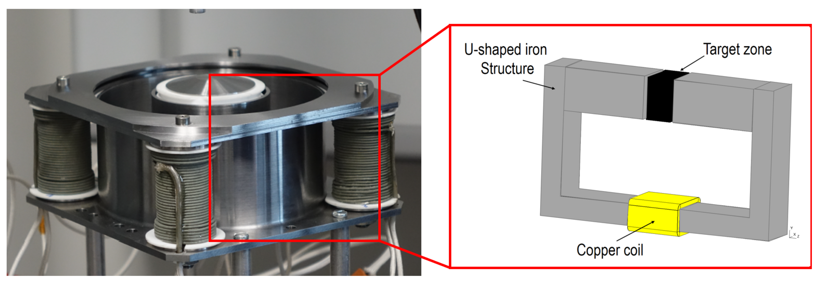
• A fixed part of the U-shaped iron structure ${\Omega }_I\setminus {\Omega }_V$ represented on Figure 1. Its dimensions are 23 cm × 14 cm × 2 cm, the thickness of the bottom hyper-rectangle containing the coil is 2 cm, and the thickness of both sides of the U-shaped circuit is 4 cm.
• A coil which is represented in yellow on Figure 1. It is made up from two bottom and top bars of 4 cm × 0.4 cm × 5 cm and two lateral bars of 2 cm × 0.4 cm × 5 cm which are linked by four curved bars. This coil is crossed by a current of 4 A and has 300 windings.
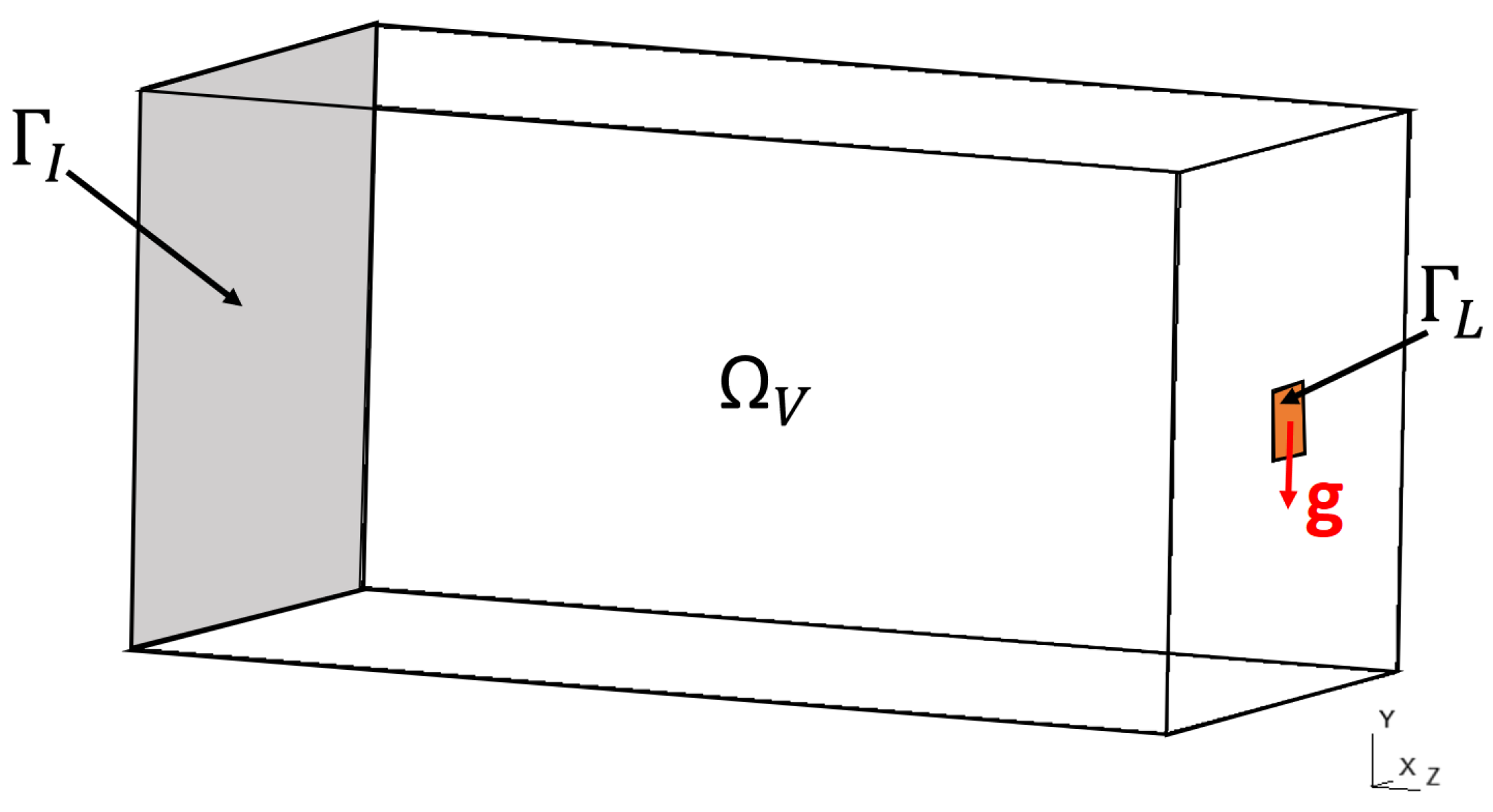
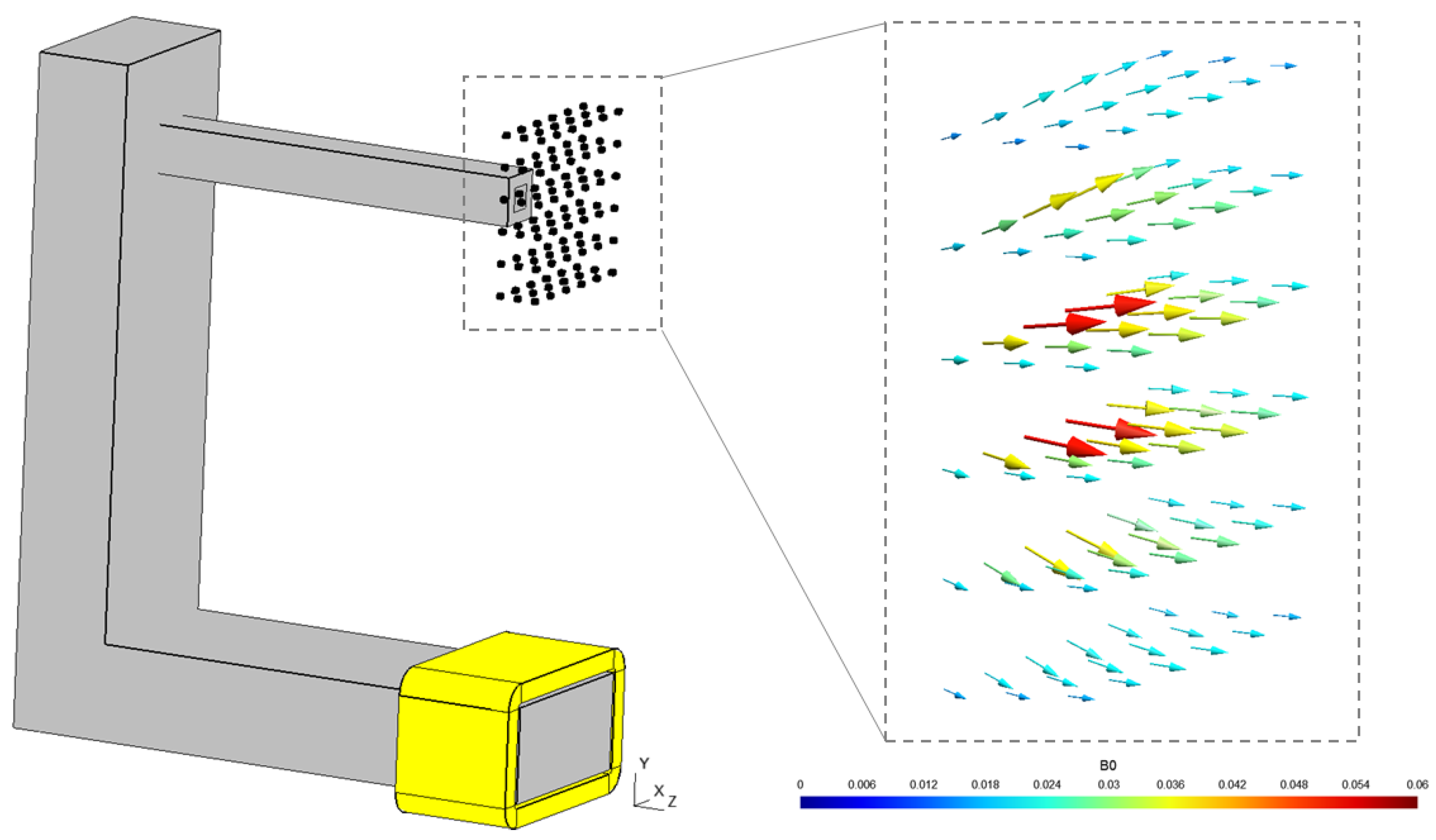
• Two design variable zones ${\Omega }_V$ which are hyper-rectangles of size 8 cm × 4 cm × 4 cm. Both of these two parts are discretized into 144,800 tetrahedrons corresponding to the finite element mesh, which contains air or ferromagnetic material. Both of these parts are subjected to a surface force of $\mathbf{g}=-1\mathbf{y}$ (N/m²) on a small surface of size 0.5 cm × 0.5 cm, as we can see in Figure 3. Note that the mechanical functions $F_2$ and ${\widehat{F}}_{3,p}$ considered in the article are linearly dependent on the amplitude of the surface force $\mathbf{g}$. Therefore, the optimal design ${\rho }^{\ast }$ obtained by minimizing one of these two functions does not depend on this amplitude. Thus, this amplitude has been arbitrarily set to 1 (N/m²).
• The target zone ${\Omega }_T$ represented in black on Figure 1 is discretized into small cubes of size 0.1 cm, as we can see on Figure 4. These cubes are centered in the air gap between the two variable hyper-rectangles. The target zone ${\Omega }_T$ is composed by $216=6\times 6\times 6$ cubes, where the magnetic flux density is evaluated.

To simplify time-consuming calculations, we consider the plane of antisymmetry of the magnetic flux density B: (Oxy), and restrict ourselves to the half-circuit shown in Figure 4.

In order to solve the main problems, see Equations (3) and (8), and the adjoint problems, defined in Equations (16) and (20), we use the FEM software GetDP (version 3.5.0, 13 May 2022)  [21] together with the finite element mesh generator Gmsh (version 4.12.2, 21 January 2024) [22,23].

For this example, the given magnetic flux density ${\mathbf{B}}_0$ in the target zone ${\Omega }_T$ is first computed using a sample ferromagnetic shape, as represented in Figure 4. This corresponds to the magnetic flux density produced by a bar of dimensions 8 cm $\times \frac{4}{3}$ cm $\times \frac{4}{3}$ cm.

In Section 4.2, Section 4.3 and Section 4.4, we aim to solve the following problems: (1) minimizing only the magnetostatic function $F_1$ without constraints and (2) minimizing the mechanical functions $F_2$ and ${\widehat{F}}_{3,p}$, respectively, with constraints on the magnetostatic function $F_1$.

To solve these topology optimization problems, a gradient-based algorithm is used. At each iteration of the optimization algorithm, the gradient is computed using the adjoint method and, hence, a descent step is obtained. In this paper, we choose to use a MATLAB (version R2021b) implementation of the MMA (method of moving asymptots) [18] solver, which is a nonlinear gradient-based optimization method. The inputs of the MMA are the objective function, the constraints, and their respective gradients.

4.2. Problem Considering Magnetostatics Only

In this section, the goal is to find the optimal distribution ${\rho }_0^{\ast }$ (discretized via Equation (22)) which minimizes the function $F_1$ given by Equation (5):

$$\left({\mathcal{P}}_1\right)\begin{array}{cc}{\mathit{\rho }}_0^{\ast }=\underset{\mathit{\rho }\in {[0,1]}^N}{arg\; min}\hfill & F_1\left(\mathit{\rho }\right)\hfill \end{array}.$$

(23)

In our case, the variable zone ${\Omega }_V$ is discretized into $N=144,800$ tetrahedrons. In order to find a design that looks like the bar in Figure 4 and which provides the target field ${\mathbf{B}}_0$, it is essential to achieve large values of the penalty parameter n used by the SIMP method (see Equation (13)). This can be explained by the very large number of iterations required for the optimization method to converge, which comes from the fact that the gradient of the function $F_1$ in the region of ${\Omega }_V$ close to the fixed iron part is very small compared to the one in the area near ${\Omega }_T$.

Note that we could have used a projection method such as one of the methods described in [24], but we have chosen to stick with the homotopy algorithm described in [9] where the penalization parameter is increased step by step. Therefore, the optimization problem is gradually forced to “chose” between 0 and 1 for each variable while ensuring that the objective function remains as low as possible.

Remark 3.

The choice of the penalty parameter n which appears in Equation (13) is challenging. Indeed, if n is very large at the start of the optimization, this leads to convergence towards a poor local minimum. Thus, we carry out a continuation process consisting of progressively increasing the penalty parameter starting from $n=3$ and increasing it by $0.5$ when, at an iteration $k+1$, $\parallel F_1\left({\mathit{\rho }}^{[k+1]}\right)-F_1\left({\mathit{\rho }}^{\left[k\right]}\right)\parallel \le {10}^{-4}$. Note that the optimization module is stopped after a fixed number of iterations (1000).

The history of convergence is shown in Figure 5 starting from the initial distribution ${\mathit{\rho }}^{\left[0\right]}=0.95$ (an almost full material distribution). This optimization results in an optimal design ${\mathit{\rho }}_0^{\ast }$ after 1000 iterations with a relative error between $\mathbf{B}\left({\mathit{\rho }}_0^{\ast }\right)$ and the target field ${\mathbf{B}}_0$ of no more than $1.5\%$ inside the target area ${\Omega }_T$, as shown by the boxplot in Figure 6 (right). Note that at the end of the optimization process, the penalty parameter reached a value $n>50$.

Although this design is close to the optimal structure (the bar in Figure 4), it still contains a lot of intermediate densities ${\rho }_i$ (corresponding to gray areas in Figure 6) near the fixed iron part ${\Omega }_I$. As such, it is not mechanically rigid. Indeed, we can notice that the left-hand side of the final structure in Figure 5 does not fit perfectly with the rest of the magnetic circuit. We will now move on to the simultaneous optimization of both the magnetic circuit’s performance and its mechanical robustness.

4.3. Problem Combining Compliance Minimization and Magnetostatics

Now that the magnetic circuit has been optimized and a first design ${\mathit{\rho }}_0^{\ast }$ has been obtained, we can move our attention to the solution of the coupled (magnetic and mechanical) problem $\left(\mathcal{P}\right)$. In this section, we thus consider the optimization of the following problem:

$$\left({\mathcal{P}}_2\right)\left\{\begin{array}{cc}\underset{\mathit{\rho }\in {[0,1]}^N}{min}\hfill & F_2\left(\mathit{\rho }\right)\hfill \\ u.c.\hfill & F_1\left(\mathit{\rho }\right)\le F_1\left({\mathit{\rho }}_0^{\ast }\right)+ϵ\hfill \end{array}\right.$$

(24)

in which $F_2$ is the compliance of the mechanical structure as defined in Equation (9) and $ϵ$ is a small value taken such that $F_1\left({\mathit{\rho }}_0^{\ast }\right)+ϵ$ corresponds to an error of $3\%$ for each cube in the target zone ${\Omega }_T$. The same algorithm as in Section 4.2 was used following the continuation method explained in Remark 3 (except that only 500 iterations are necessary). Figure 7 shows the evolution of the objective function $F_2$ and constraint $F_1$ over the course of the optimization process.

Comparing the evolution of the structure in both Figure 5 and Figure 7 (top), we can see that both optimizations start by designing the right-hand side of the structure. However, after a hundred or so iterations, the two optimized structures begin to diverge significantly from each other, with the coupled optimization resulting in the appearance of two slabs connecting the right optimized area to the mechanically fixed iron part on the left. The final design is then close to the classical topology-optimized “cantilever” structure [1]. The resulting field from the optimal structure can be seen in Figure 8. The relative error inside ${\Omega }_T$ has naturally increased (the maximum error is now 5%) but its mechanical rigidity has greatly improved.

Minimizing compliance has increased the rigidity of the structure. Nevertheless, minimizing the compliance does not strictly ensure the mechanical strength of the part. Indeed, the real criteria for mechanical strength is the von Misses stress (for ductile materials): the material is robust if the von Misses stress does not exceed the yield point of the material. That is why we are now going to look at the direct optimization of the von Mises stress.

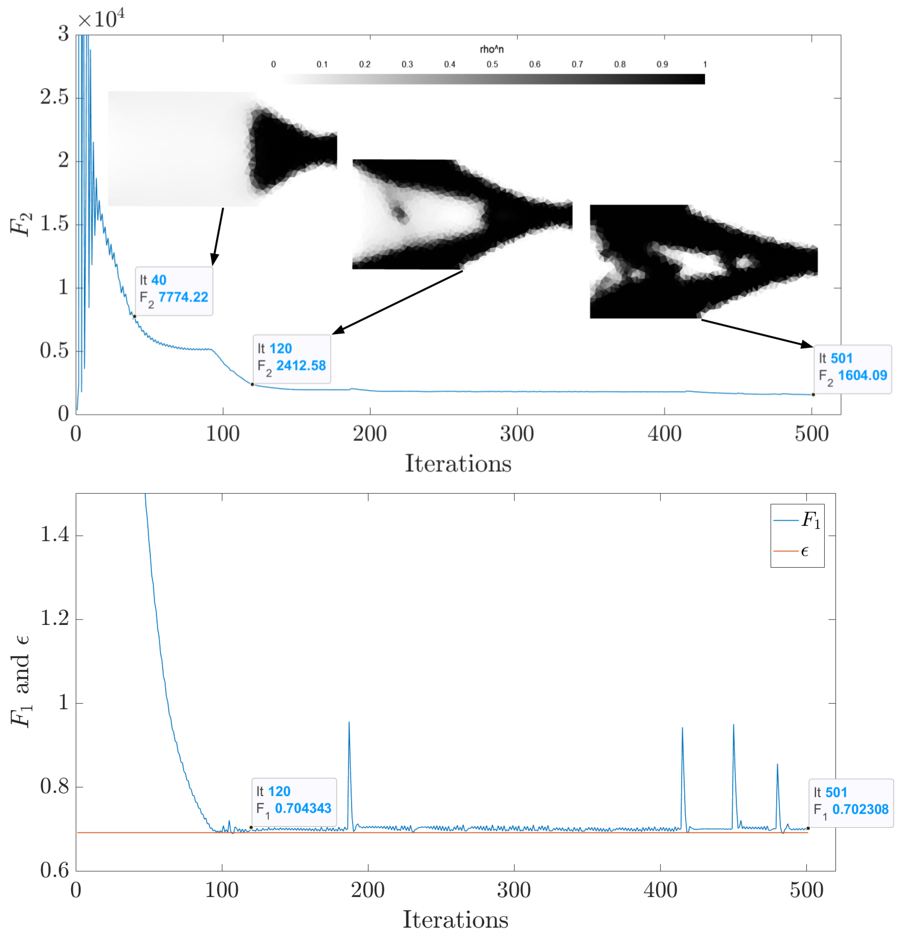
4.4. Problem Combining Global Stress Measure Minimization and Magnetostatics

In this section, we will solve the following optimization problem:

$$\left({\mathcal{P}}_3\right)\left\{\begin{array}{cc}\underset{\mathit{\rho }\in {[0,1]}^N}{min}\hfill & {\widehat{F}}_{3,p}\left(\mathit{\rho }\right)\hfill \\ u.c.\hfill & F_1\left(\mathit{\rho }\right)\le F_1\left({\mathit{\rho }}_0^{\ast }\right)+ϵ\hfill \end{array}\right.$$

(25)

where ${\widehat{F}}_{3,p}$ is the global measure of the relaxed stress function defined in Equation (14). The parameter p is set equal to 6 and $ϵ$ is the same value as in the previous Section 4.3.

Figure 9 shows the evolution of the objective function ${\widehat{F}}_{3,p}$ and constraint $F_1$, respectively, over the course of the iterations. The field associated with the final design is shown in Figure 10.

Once again, we can see significant differences between this design and the one previously obtained for the compliance minimization with a much finer shape joining the top and bottom slabs. We now have a relative magnetic error of no more than $4\%$ in the target zone ${\Omega }_T$. In detail, Figure 11 shows the von Mises stress inside the optimized design of $\left({\mathcal{P}}_2\right)$ and $\left({\mathcal{P}}_3\right)$. If the objective function is the compliance ($F_2$), then the stress measure is higher and more concentrated than the case where the objective function is the relaxed von Mises stress (${\widehat{F}}_{3,p}$), which leads to a more uniform distribution of $\rho {\sigma }_{VM}$.

5. Conclusions

In this paper, we have extended topology optimization based on the adjoint method and the SIMP methodology to address 3D design problems involving both magnetic and mechanical considerations. This coupled optimization proved interesting for achieving manufacturable designs, as a first optimization without taking mechanical considerations into account showed that the magnetic circuit could break if any force acted on it. We implemented two methods to maximize the mechanical rigidity of the structure. The first, based on the compliance of structure, resulted in a rigid design but with locally high stress. The second, based on the maximal von Mises stress, resulted in locally robust designs while maintaining good magnetic performance.

References

1. Allaire, G.; Schoenauer, M. Conception Optimale de Structures; Springer: Berlin, Germany, 2007; Volume 58. [Google Scholar]
2. Bendsoe, M.P.; Sigmund, O. Topology Optimization: Theory, Methods, and Applications; Springer Science & Business Media: Berlin/Heidelberg, Germany, 2003. [Google Scholar]
3. Sigmund, O. Morphology-based black and white filters for topology optimization. Struct. Multidiscip. Optim. 2007, 33, 401–424. [Google Scholar] [CrossRef]
4. Bendsøe, M.P.; Sigmund, O. Material interpolation schemes in topology optimization. Arch. Appl. Mech. 1999, 69, 635–654. [Google Scholar] [CrossRef]
5. Sanogo, S.; Messine, F.; Henaux, C.; Vilamot, R. Topology optimization for magnetic circuits dedicated to electric propulsion. IEEE Trans. Magn. 2014, 50, 1–13. [Google Scholar] [CrossRef]
6. Gauthey, T.; Gangl, P.; Hassan, M.H. Multi-material topology optimization with continuous magnetization direction for permanent magnet synchronous reluctance motors. arXiv 2021, arXiv:2107.04825. [Google Scholar]
7. Youness, R.; Messine, F. An implementation of adjoint-based topology optimization in magnetostatics: Application to design hall-effect thrusters. COMPEL-Int. J. Comput. Math. Electr. Electron. Eng. 2019, 38, 1023–1035. [Google Scholar] [CrossRef]
8. Cherrière, T.; Laurent, L.; Hlioui, S.; Louf, F.; Duysinx, P.; Geuzaine, C.; Ben Ahmed, H.; Gabsi, M.; Fernández, E. Multi-material topology optimization using Wachspress interpolations for designing a 3-phase electrical machine stator. Struct. Multidiscip. Optim. 2022, 65, 352. [Google Scholar] [CrossRef]
9. Houta, Z.; Messine, F.; Huguet, T. Topology Optimization for Magnetic Circuits with Adjoint Method in 3D. COMPEL 2023. Available online: https://hal.science/hal-04095069v2 (accessed on 10 March 2024).
10. Gangl, P.; Amstutz, S.; Langer, U. Topology optimization of electric motor using topological derivative for nonlinear magnetostatics. IEEE Trans. Magn. 2015, 52, 7201104. [Google Scholar] [CrossRef]
11. Brun, O.; Chadebec, O.; Ferrouillat, P.; Niyonzima, I.; Luo, Z.; Le Floch, Y.; Siau, J.; Vi, F.; Gerbaud, L. A Level-Set Based Topology Optimization for Maximizing the Torque of Switch Reluctance Machines. In Proceedings of the 24th International Conference on the Computation of Electromagnetic Fields (Compumag’2023), Kyoto, Japan, 22–26 May 2023. [Google Scholar]
12. Cherrière, T. Élaboration de Méthodes et d’Outils Logiciels pour l’Optimisation Topologique Magnéto-Mécanique de Machines Électriques Tournantes. Ph.D. Thesis, Université Paris-Saclay, Paris, France, 2023. [Google Scholar]
13. Rossi, A.; Messine, F.; Hénaux, C. Parametric optimization of a Hall Effect Thruster magnetic circuit. Trans. Jpn. Soc. Aeronaut. Space Sci. Aerosp. Technol. Jpn. 2016, 14, 197–202. [Google Scholar] [CrossRef] [PubMed]
14. Cheng, G.; Guo, X. ϵ-Relaxed Approach in Structural Topology Optimization. Struct. Optim. 1997, 13, 258–266. [Google Scholar] [CrossRef]
15. Céa, J. Conception optimale ou identification de formes, calcul rapide de la dérivée Directionnelle de la Fonction coût. M2AN-Model. Math. Anal. Numer. 1986, 20, 371–402. [Google Scholar] [CrossRef]
16. Lukáš, D. An Integration of Optimal Topology and Shape Design for Magnetostatics. In Scientific Computing in Electrical Engineering; Springer: Berlin/Heidelberg, Germany, 2006; pp. 227–232. [Google Scholar]
17. Le, C.; Norato, J.; Bruns, T.; Ha, C.; Tortorelli, D. Stress-based topology optimization for continua. Struct. Multidiscip. Optim. 2010, 41, 605–620. [Google Scholar] [CrossRef]
18. Svanberg, K. The method of moving asymptotes—A new method for structural optimization. Int. J. Numer. Methods Eng. 1987, 24, 359–373. [Google Scholar] [CrossRef]
19. Li, L.; Khandelwal, K. Volume preserving projection filters and continuation methods in topology optimization. Eng. Struct. 2015, 85, 144–161. [Google Scholar] [CrossRef]
20. Guest, J.K.; Prévost, J.H.; Belytschko, T. Achieving minimum length scale in topology optimization using nodal design variables and projection functions. Int. J. Numer. Methods Eng. 2004, 61, 238–254. [Google Scholar] [CrossRef]
21. Dular, P.; Geuzaine, C. GetDP Reference Manual. 2024. Available online: https://getdp.info/dev/doc/texinfo/getdp.pdf (accessed on 10 March 2024).
22. Geuzaine, C.; Remacle, J.F. Gmsh: A 3-D finite element mesh generator with built-in pre-and post-processing facilities. Int. J. Numer. Methods Eng. 2009, 79, 1309–1331. [Google Scholar] [CrossRef]
23. Remacle, J.F.; Geuzaine, C. Gmsh Reference Manual. 2024. Available online: https://gmsh.info/dev/doc/texinfo/gmsh.pdf (accessed on 10 March 2024).
24. Lucchini, F.; Torchio, R.; Cirimele, V.; Alotto, P.; Paolo, B. Topology Optimization for Electromagnetics: A Survey. IEEE Access 2022, 10, 98593–98611. [Google Scholar] [CrossRef]
Figure 1. (left) A Hall-effect thruster whose shape must be optimized to obtain a target magnetic field B 0 inside the cavity. (right) A cross-section of this device is approximated into the following “toy” problem: a U-shaped iron structure is obtained (the coil was moved down from one side of the thruster to the center of the structure) with a cubic target zone in which the field must be controlled.
Mathematics 12 01147 g001
Figure 2. Half of the magnetic circuit studied in this article (the other half is obtained by symmetry), and the different domains that make it up: the iron domain Ω I , the coil Ω C , the air Ω A , the target area Ω T , and the variable region Ω V , in which we will optimize the structure.
Mathematics 12 01147 g002
Figure 3. Zoom in on the Ω V region in which we are searching for the optimal shape of the iron structure and the different notations used to simulate its mechanical deformation: Γ I is a fixed surface on which the structure is clamped and Γ L the surface on which a load g is applied.
Mathematics 12 01147 g003
Figure 4. Material distribution providing the magnetic flux density B 0 and zoom on this magnetic flux density B 0 on the target zone.
Mathematics 12 01147 g004
Figure 5. Evolution of the objective function F 1 during the optimization process described in Section 4.2 to solve problem ( P 1 ) . The small peaks correspond to the increase in the penalty parameter n.
Mathematics 12 01147 g005
Figure 6. (left) Magnetic field inside the simulation domain for ρ 0 . (right) Boxplot of the relative error B ( ρ 0 ) B 0 / B 0 between these two fields inside the 216 cubes which discretize Ω T (as explained in Section 4.1).
Mathematics 12 01147 g006
Figure 7. (top) Evolution of the objective function F 2 during the optimization process described in Section 4.3 to solve ( P 2 ) . (bottom) Same for the constraint F 1 .
Mathematics 12 01147 g007
Figure 8. Same as in Figure 6 for the optimal structure resulting from the optimization of (24).
Mathematics 12 01147 g008
Figure 9. (top) Evolution of the objective function F ^ 3 , p during the optimization process described in Section 4.3 to solve ( P 2 ) . (bottom) Same for the constraint F 1 .
Mathematics 12 01147 g009
Figure 10. Same as in Figure 6 for the optimal structure resulting from the optimization of (25).
Mathematics 12 01147 g010
Figure 11. (left) Relaxed von Mises stress distribution of the solution of problem (24). (right) Same for the solution of problem (25).
Mathematics 12 01147 g011
Disclaimer/Publisher’s Note: The statements, opinions and data contained in all publications are solely those of the individual author(s) and contributor(s) and not of MDPI and/or the editor(s). MDPI and/or the editor(s) disclaim responsibility for any injury to people or property resulting from any ideas, methods, instructions or products referred to in the content.