Robust Design Optimization of Electric Machines with Isogeometric Analysis

Abstract

In electric machine design, efficient methods for the optimization of the geometry and associated parameters are essential. Nowadays, it is necessary to address the uncertainty caused by manufacturing or material tolerances. This work presents a robust optimization strategy to address uncertainty in the design of a three-phase, six-pole permanent magnet synchronous motor (PMSM). The geometry is constructed in a two-dimensional framework within MATLAB^®, employing isogeometric analysis (IGA) to enable flexible shape optimization. The main contributions of this research are twofold. First, we integrate shape optimization with parameter optimization to enhance the performance of PMSM designs. Second, we use robust optimization, which creates a min–max problem, to ensure that the motor maintains its performance when facing uncertainties. To solve this bilevel problem, we work with the maximal value functions of the lower-level maximization problems and apply a version of Danskin’s theorem for the computation of generalized derivatives. Additionally, the adjoint method is employed to efficiently solve the lower-level problems with gradient-based optimization. The paper concludes by presenting numerical results showcasing the efficacy of the proposed robust optimization framework. The results indicate that the optimized PMSM designs not only perform competitively compared to their non-robust counterparts but also show resilience to operational and manufacturing uncertainties, making them attractive for industrial applications.

1. Introduction

The growing importance of electric machines in transportation and other applications necessitates highly optimized designs. This trend is clearly seen in the shift towards electric vehicles in the automotive industry. This has become especially significant in efforts to mitigate climate change and promote environmental sustainability. Over the past decade, the development of electric machines has shifted from physical to virtual prototypes, driven by advancements in numerical simulation. This change has resulted in cost savings and reduced material usage, improving sustainability. To further exploit these benefits, the current trend is to move from a purely numerical simulation-based procedure to one that improves the performance through optimization methods that are able to handle many design variables.

Such optimization processes in the design of electric machines aim to balance competing objectives such as high torque capacity, operational smoothness and cost-effectiveness [1,2]. However, one major challenge is uncertainties during manufacturing, which can affect the performance and efficiency in a negative way or even lead to the failure [3] of the electric machine. In order to ensure a reliable design, it is advisable to account for these uncertainties in the design optimization process using robust optimization methods that account for these variations.

The field of electric machine optimization encompasses a wide range of specialized studies. In the optimization of electric machines, there exist two main approaches: gradient-based algorithms and gradient-free methods, like particle swarm optimization (PSO). The latter are non-intrusive but require many simulation runs and are thus time-consuming [4]. In this paper, we choose a gradient-based optimization approach and seek to obtain robust optima with a moderate number of optimization runs. In the field of gradient-based optimization, much research has been devoted to advancing free-form optimization using the finite element method (FEM) and variants thereof (such as isogeometric analysis (IGA)), which has led to a reduction in torque ripple [1,5]. Alongside these, there has been a focus on parameter optimization with different performance metrics, such as the magnet mass [6,7]. However, there is a noticeable gap in research that concurrently addresses both free-shape and parameter optimization and their combined effects on electric machine performance. Only a few studies have appeared at this intersection, using FEM for their investigations [8]. In contrast to these methods, our study [9] introduces a gradient-based optimization framework within the IGA context, combining both parameter and shape optimization. This approach, supported by numerical evidence, outperforms the sequential optimization, which first addresses the parameters and then the shape. Additionally, the discretization technique employed in [9] provides several benefits, particularly for free-form optimization [10].

The objective of this paper is to build on these results and extend our previously established gradient-based optimization methodology, which combines parameter and free-shape design variables in IGA, by introducing a robustoptimization formulation. We deal with uncertainties using the worst-case optimization method originally proposed by Ben-Tal [11]. In the literature, the worst-case approach for robustification against uncertainties has been already successfully applied for a three-phase, six-pole PMSM, where both uncertainties and optimization variables are parameters [3]. Notably, these studies employed the standard FEM for their discretization and only addressed parameter optimization; they did not consider free-form optimization. In contrast, the present study generalizes this robust optimization approach by allowing a wider set of design variables on an electric motor that is simulated with state of the art techniques to handle rotation, i.e., mortaring [12].

A novel aspect of this research is the inclusion of uncertainties in both the motor parameters and its shape, and the consideration of both as variables in the optimization process. To improve the efficiency, we utilize IGA instead of the conventional FEM in discretizing the PDE. The robust approach results in a min–max optimization problem, where objective function and critical constraints are replaced by the maximum over an uncertainty set. To solve this, we employ a generalization of Danskin’s theorem [13], which yields an efficient tool to compute generalized derivatives of the resulting robustified objective function and constraints under mild assumptions. The approach’s advantage is that it only requires first derivatives. However, it is crucial to note that the outer minimization problem can become non-smooth. This property necessitates the use of a non-smooth optimization solver to ensure convergence to a non-smooth optimum; see also the discussion in Bertsimas et al. [14].

The rest of this paper is structured as follows. Section 2 introduces the mathematical and physical foundations with a focus on the relevant aspects for the optimization. In Section 3, the robust optimization method and its application to the optimal design of a PMSM are described. Section 4 presents numerical results for the robust shape and parameter optimization of a PMSM. Section 5 summarizes the main results and explores possible directions for future research.

2. Physical Model

2.1. Geometry Representation

This section introduces the physical model and the computational methods that we use for our optimization techniques. Figure 1 shows the motor model that will be used in this paper. The colors of the motor represent the materials used, i.e., gray for iron, blue for air, red for copper and green for the magnet, where the magnetization direction is shown by the arrows. The copper represents stranded conductor windings, where the phase and current direction are indicated. Note that the motor is modeled with two small air gaps at the rotor iron bridges to represent saturation effects and allowing linear material properties to be used. In 2005, Hughes et al. introduced IGA, which we use to discretize the physical domain and the PDE [15]. Unlike the standard FEM, which uses polynomials as basis functions, IGA uses B-splines and non-uniform rational B-splines (NURBS) [16]. The flexibility provided by spline functions is essential in accurately representing conic sections while maintaining computational efficiency. This feature is particularly useful in simulating rotating machines.

The formulation of the univariate B-spline basis functions $N_i^p$ of degree p is expressed by a knot vector:

$$\mathsf{\Xi }=\{{\xi }_1,{\xi }_2,\dots ,{\xi }_{n+p+1}\},$$

where the knots ${\xi }_i$ define the support of the basis functions. These functions are computed through a recursive process, utilizing Cox–de Boor’s recursion formula [17], which is given by

$$N_i^p\left(\xi \right)=\frac{\xi -{\xi }_i}{{\xi }_{i+p}-{\xi }_i}{N}_i^{p-1}\left(\xi \right)+\frac{{\xi }_{i+p+1}-\xi }{{\xi }_{i+p+1}-{\xi }_{i+1}}{N}_{i+1}^{p-1}\left(\xi \right),$$

(1)

$$N_i^0\left(\xi \right)=\left\{\begin{array}{cc}1\hfill & \mathrm{if}{\xi }_i\le \xi <{\xi }_{i+1}\hfill \\ 0\hfill & \mathrm{otherwise}.\hfill \end{array}\right.$$

These basis functions have useful mathematical properties, such as the partition of unity, compact support of the basis function and pointwise positivity, which make them suitable for approximating geometries. A comprehensive discussion of these properties can be found in the work of Hughes et al. [15]. The two-dimensional domain in our work is constructed using the tensor-product method, which allows for the creation of multivariate B-splines or NURBS. This method involves the multiplication of individual basis functions from each parametric coordinate, thus forming a set of multivariate basis functions. This approach provides an efficient framework and can be also extended for the construction of three-dimensional domains [15]. To precisely map the parametric domain $\widehat{\Omega }\in {(0,1)}^d$ to the physical domain $\Omega \subseteq {\mathbb{R}}^r$, where $r\ge d$, we use geometric basis functions ${\widehat{G}}_k$, which can be either B-splines or NURBS. Each of these basis functions ${\widehat{G}}_k$ is multiplied with the corresponding control point ${\mathbf{C}}_k$. This leads to the mapping $\mathrm{F}:\widehat{\Omega }\to \Omega$ defined by

$$\mathrm{F}\left(\widehat{\mathbf{x}}\right)=\sum _k{\widehat{G}}_k\left(\widehat{\mathbf{x}}\right){\mathbf{C}}_k.$$

(2)

Here, $\widehat{\mathbf{x}}$ is located within the parametric domain $\widehat{\Omega }$ and $\mathrm{F}\left(\widehat{\mathbf{x}}\right)$ is the corresponding point in the physical domain $\Omega$. The mapping defined in (2) must satisfy some regularity conditions, e.g., it must be a diffeomorphism, which is required for the application of the transformation formula for integrals [18]. A visual representation of the relationship between the control points and the model’s geometry is shown in Figure 2.

Shifting the position of a control point ${\mathbf{C}}_k$ results in a corresponding change in the geometry according to the mapping (2). Therefore, the transformation (2) can be used directly for shape optimization, which is a convenient feature of IGA. For geometries that are complex in their topology or material distribution, such as the rotor and stator in Figure 1, multipatch decomposition is necessary. This method divides the overall domain into several contiguous patches and couples the control points of neighboring patches to ensure continuity; see [20]. The grey lines in Figure 1 indicate the boundaries of the images of the patches.

2.2. Governing Equations

In this subsection, we describe the physical system governing PMSMs [12]. It is based on the magnetostatic approximation of Maxwell’s equations. This simplification is justified and often used when electric machines operate at a low frequency, since, in this case, the displacement currents and eddy currents are negligible compared to the source current. This assumption simplifies our model to an elliptic PDE, which can be expressed in terms of the magnetic vector potential $\mathbf{A}$ as follows:

$$\nabla \times \left(\nu \nabla \times \mathbf{A}\right)={\mathbf{J}}_{\mathrm{source}}+\nabla \times \left(\nu {\mathbf{B}}_{\mathrm{r}}\right).$$

(3)

In (3), the term $\mathbf{B}=\nabla \times \mathbf{A}$ denotes the magnetic flux density, while $\nu$ represents the material’s linear reluctivity. The term ${\mathbf{J}}_{\mathrm{source}}$ is the density of the current source, and ${\mathbf{B}}_{\mathrm{r}}$ is the remanent magnetic flux density from the permanent magnets, which follows from the constitutive material law [21]. For a more detailed understanding of these physical principles, see [22,23]. According to Helmholtz’s theorem, $\mathbf{A}$ is not uniquely determined by the PDE. To simplify the model, ensure its uniqueness and reduce the computational cost, it is common to reduce (3) to a two-dimensional problem by assuming a substantial axial length of the motor. This step divides the computational area into the 2D rotor and 2D stator sections, ${\Omega }_{\mathrm{R}}$ and ${\Omega }_{\mathrm{S}}$, respectively, and leads to the elliptic PDE in 2D,

$$\begin{array}{cccc}\hfill \nabla ·\left(\nu \nabla A_{z,\mathrm{R}}\right)& =\nu \nabla ·{\mathbf{B}}_r^{\perp },\hfill & \hfill & \mathrm{in}{\Omega }_{\mathrm{R}}\hfill \\ \hfill \nabla ·\left(\nu \nabla A_{z,\mathrm{S}}\right)& =-J_{\mathrm{z},\mathrm{source}}\hfill & \hfill & \mathrm{in}{\Omega }_{\mathrm{S}},\hfill \end{array}$$

(4)

where only the $A_z$-component of the magnetic vector potential is considered. This component is separated for the rotor and stator, denoted as $A_{z,\mathrm{R}}$ and $A_{z,\mathrm{S}}$. In electric machine modeling, boundary conditions play a critical role. For the Dirichlet boundary, denoted as ${\mathsf{\Gamma }}_{\mathrm{d}}$, which is located at the outer boundaries of the stator and rotor—see Figure 1—the condition $A_z=0$ is imposed. On the boundary ${\mathsf{\Gamma }}_{\mathrm{ap}}$, antiperiodic conditions are implemented due to the simulation and optimization being applied to only one pole of the entire motor. For the coupling interface ${\mathsf{\Gamma }}_{\mathrm{ag}}$ between the rotor and stator, the following conditions must be met:

$$\begin{array}{cc}\hfill A_{z,\mathrm{S}}\left(\theta \right)& =A_{z,\mathrm{R}}(\theta -\alpha ),\hfill \\ \hfill H_{\theta ,\mathrm{S}}\left(\theta \right)& =H_{\theta ,\mathrm{R}}(\theta -\alpha ),\hfill \end{array}$$

(5)

where $\mathbf{H}=\nu \mathbf{B}$ denotes the magnetic field strength, with $\mathbf{B}$ as the magnetic flux density, and both $A_z$ and $H_{\theta }$ are evaluated in their respective rotor or stator local coordinate systems in dependence on the rotation angle $\alpha$. This ensures the continuity of the magnetic vector potential $A_z$ and the azimuthal magnetic field strength $H_{\theta }$ across ${\mathsf{\Gamma }}_{\mathrm{ag}}$ [24]. A visualization of the the boundary conditions can be found in Figure 1. From the 2D reduction, the reduced remanence ${\mathbf{B}}_r^{\perp }$ is expressed as

$${\mathbf{B}}_r^{\perp }=B_{\mathrm{r}}\left(\begin{array}{c}-\sin \left(\varphi \right)\\ \cos \left(\varphi \right)\end{array}\right),$$

(6)

where $B_{\mathrm{r}}$ is the remanence magnitude and $\varphi$ is the magnet direction angle, defining the orientation of the magnet’s remanence in the two-dimensional plane. The source current density in the k-th winding is defined as

$$J_{\mathrm{z},\mathrm{source}}^{\left(k\right)}=\frac{I_{\mathrm{app}}{n}_{\mathrm{wind}}}{A_{\mathrm{coil}}}\sin \left(P\alpha +{\theta }_{\mathrm{current}}+\frac{2\pi }{3}k\right),k\in \{0,1,2\},$$

(7)

and is zero outside the k-th winding. The synchronous operation of the motor implies that the time dependency in (7) is represented by the rotor angle $\alpha$, adjusted by the number of pole pairs P. In (7), $n_{\mathrm{wind}}$ denotes the number of windings in each coil. $I_{\mathrm{app}}$ represents the application current, which is the primary source of electromagnetic field generation in the system, and $A_{\mathrm{coil}}$ refers to the cross-sectional area of the coil, which affects both the material usage and electromagnetic performance. The total current density $J_{\mathrm{z},\mathrm{source}}$ is the sum over all windings,

$$J_{\mathrm{z},\mathrm{source}}=\sum _k{J}_{\mathrm{z},\mathrm{source}}^{\left(k\right)}$$

and is assumed to be evenly distributed within the coils.

2.3. Discretization

In this subsection, we focus on the IGA discretization of the governing Equation (4). To apply a Ritz–Galerkin method, we introduce ansatz and test spaces, both spanned by a basis $N\left(\mathbf{x}\right)$, which is defined in (1):

$$\begin{array}{cccc}\hfill A_z\left(\mathbf{x}\right)\approx u\left(\mathbf{x}\right)& =\sum _j{N}_j\left(\mathbf{x}\right)u_j,\hfill & \hfill v\left(\mathbf{x}\right)& =\sum _i{N}_i\left(\mathbf{x}\right)v_i.\hfill \end{array}$$

(8)

Deriving the weak formulation of (4) and inserting the ansatz and test function expansions from  (8), we obtain the system of equations

$$\left(\begin{array}{ccc}{\mathbf{K}}_{\mathrm{R}}& \mathbf{0}& -{\mathbf{G}}_{\mathrm{R}}\\ \mathbf{0}& {\mathbf{K}}_{\mathrm{S}}& {\mathbf{G}}_{\mathrm{S}}{\mathbf{R}}_{\alpha }\\ -{\mathbf{G}}_{\mathrm{R}}^{\top }& {\mathbf{R}}_{\alpha }^{\top }{\mathbf{G}}_{\mathrm{S}}^{\top }& \mathbf{0}\end{array}\right)\left(\begin{array}{c}{\mathbf{u}}_{\mathrm{R},\alpha }\\ {\mathbf{u}}_{\mathrm{S},\alpha }\\ {\mathbf{\lambda }}_{\alpha }\end{array}\right)=\left(\begin{array}{c}{\mathbf{b}}_{\mathrm{R},\alpha }\\ {\mathbf{b}}_{\mathrm{S},\alpha }\\ \mathbf{0}\end{array}\right).$$

(9)

Equation (9) is a coupled system of discretized elliptic PDEs. The stiffness matrices ${\mathbf{K}}_{\mathrm{R}}$, ${\mathbf{K}}_{\mathrm{S}}$ and right-hand sides ${\mathbf{b}}_{\mathrm{R}}$, ${\mathbf{b}}_{\mathrm{S}}$ for the rotor and stator are obtained in a standard way from the weak formulation of the elliptic PDEs (4). The coupling matrices ${\mathbf{G}}_{\mathrm{R}}$ and ${\mathbf{G}}_{\mathrm{S}}$ result from the application of harmonic (Fourier) test functions in a mortaring approach to discretize the coupling conditions (5), as detailed in [12]. For distinct rotation angles $\alpha \in \{{\alpha }_0,{\alpha }_1,\dots ,{\alpha }_{N-1}\}$, the stator coupling matrix ${\mathbf{G}}_{\mathrm{S}}$ is multiplied by a rotation matrix ${\mathbf{R}}_{\alpha }$. This matrix contains block diagonal entries of sine and cosine functions, thereby eliminating the need for the reassembly of the coupling matrix for each $\alpha$. This improves the computational efficiency when evaluating multiple rotation angles [24]. For more details about the discretization procedure, see [9]. In (9), the right-hand side and the rotation matrix depend on the rotation angle $\alpha$ and consequently also the solution $({\mathbf{u}}_{\mathrm{R},\alpha },{\mathbf{u}}_{\mathrm{R},\alpha },{\mathbf{\lambda }}_{\alpha })$. Taking advantage of the symmetry of the three-phase current, we consider only the angles $\alpha \in \{0,1,\dots ,19\}$ degrees.

In order to evaluate the performance of the system, we solve (9) and compute the torque $T_{\alpha }\left(\mathbf{u}\right)$ based on energy conservation principles [24] by

$$T_{\alpha }\left(\mathbf{u}\right)=-L{\mathbf{u}}_{\mathrm{S},\alpha }^{\top }{\mathbf{G}}_{\mathrm{S}}{\mathbf{R}}_{\alpha }^{\prime }{\mathbf{\lambda }}_{\alpha }.$$

(10)

Here, ${\mathbf{R}}_{\alpha }^{\prime }$ is the derivative of the rotation matrix ${\mathbf{R}}_{\alpha }$ with respect to the rotation angle $\alpha$. Since the computation is done in 2D, we include the axial length L directly in the calculation of the torque $T_{\alpha }\left(\mathbf{u}\right)$. To determine the average torque performance, we need to solve the linear system (9) for each angle $\alpha$, since satisfying a predefined average torque will be a constraint in the optimization.

3. Optimization

In the literature on the optimization of electric machines, various performance aspects are important. We summarize the most important objective functions that are considered in [19]. A major focus, especially for industrial applications, is the cost-effective use of materials. For machines using permanent magnets, reducing the size of the magnet is a critical goal, because these magnets are made of rare earth materials, which are costly and have large environmental footprints [25]. A critical constraint is to keep the average torque at a certain level because the cost and environmental impact increase as more permanent magnet material is used. Another important goal is to reduce torque ripple, which helps to lower vibration and noise. These objectives have, for example, been studied in [2,5,6]. However, in the optimization of electric machines, the focus has been on either parameter optimization or free-form optimization. There is less work on combining these two approaches, e.g., [8,9]. However, combining the two promises better results because it offers more design freedom.

For practical design optimization problems, often, several objective functions are of interest, which leads to a multiobjective optimization problem. Here, we consider two competing objective functions and apply the weighted sum approach; see [26]. The first objective function is the area of the permanent magnets $A_{\mathrm{mag}}$, contributing mainly to parameter optimization, and the second is the standard deviation $\widehat{T}$ of the torque, associated with free-shape optimization. The area $A_{\mathrm{mag}}$ of the permanent magnet is computed as the product of the width and the height of the region highlighted in green in Figure 1. For the torque evaluation, the standard deviation $\widehat{T}$ and the mean torque $T_{\mathrm{mean}}$ are calculated based on the torque (10) for a discrete set of rotation angles $\alpha$ by

$$T_{\mathrm{mean}}=\frac{1}{N}\sum _{\alpha }{T}_{\alpha },\widehat{T}=\sqrt{\frac{1}{N}\sum _{\alpha }{\left(T_{\alpha }-T_{\mathrm{mean}}\right)}^2}.$$

(11)

In our optimization, the mean torque $T_{\mathrm{mean}}$ is constrained to be at least a predetermined minimum level $T_{\mathrm{desired}}$. This constraint affects the required size of the permanent magnet. Altogether, the combined parameter and shape optimization problem is defined as

$$\begin{array}{cc}\hfill \underset{\mathbf{u},\mathit{p}}{\min }& F(\mathbf{u},\mathit{p})=m_1{A}_{\mathrm{mag}}+m_2\widehat{T}\hfill \\ \hfill \mathrm{s}.\mathrm{t}.& \mathbf{e}(\mathbf{u},\mathit{p})=\mathbf{0},\hfill & \hfill (\mathrm{State}\mathrm{Equation})\\ \hfill & T_{\mathrm{mean}}\ge T_{\mathrm{desired}},\hfill & \hfill (\mathrm{Torque}\mathrm{Constraint})\\ \hfill & \mathbf{0}\le \mathit{p}\le \mathbf{1},\hfill & \hfill (\mathrm{Design}\mathrm{Bounds})\\ \hfill & \mathbf{g}\left(\mathit{p}\right)\le \mathbf{0}.\hfill & \hfill (\mathrm{Geometric}\mathrm{Feasibility})\end{array}$$

(12)

Here, $m_1$ and $m_2$ are weighting factors introduced to balance the components of the objective function. The state equation $\mathbf{e}(\mathbf{u},\mathit{p})=\mathbf{0}$ represents the governing equations of the system (9). $\mathit{p}$ are the optimization variables, including both shape and further design parameters. In our case, $\mathit{p}$ will consist of control points located on the air gap, the geometric parameters of the permanent magnet and the electric phase angle. Further explanation of the optimization variables is given in Section 4. Numerical results for another electric machine and without the consideration of uncertainty are presented in [9,27] and demonstrate that the combined parameter and shape optimization is able to reduce the torque ripple significantly while also reducing the size of the magnets.

Robust Optimization

As described in Section 1, the goal of this paper is to make the optimization problem (12) robust to uncertainties. Uncertainties are inevitable in real-world scenarios and can affect the model parameters $\mathit{q}$ as well as the design variables $\mathit{p}$. In our case, we consider uncertainty in the application current $I_{\mathrm{app}}$ and in the position of the control points that define the shape of the machine’s air gap. Therefore, we introduce the vector $\mathit{w}=(\mathit{\delta }\mathit{p},\mathit{q})\in {\mathbb{R}}^{n_p}\times {\mathbb{R}}^{n_q}$ to represent the uncertainty in the system and apply a robust optimization approach [11]. A comprehensive overview of robust nonlinear optimization can be found in [28].

We define a closed, convex and bounded uncertainty set that contains all relevant realizations of the uncertain quantities. This set accounts for uncertainties in both parameters and optimization variables. During optimization without uncertainties, the model parameters are fixed. However, the fixed values impact the optimized design. Individual sets represent uncertainties, and the combined uncertainty set is the Cartesian product of these individual sets.

• Uncertainty set for parameters:

  $$U_{p,2}=\left\{\mathit{\delta }\mathit{p}\in {\mathbb{R}}^{n_p}\mid \mathit{\delta }\mathit{p}={\mathit{R}}_p{\mathit{v}}_p,{\parallel {\mathit{v}}_p\parallel }_2\le 1\right\}$$

  with ${\mathit{R}}_p\in {\mathbb{R}}^{n_p,m_p}$, $m_p\le n_p$, $\mathrm{rank}\left({\mathit{R}}_p\right)=m_p$.
• Uncertainty set for design variables:

  $$U_{q,2}=\left\{\mathit{q}\in {\mathbb{R}}^{n_q}\mid \mathit{q}=\widehat{\mathit{q}}+{\mathit{R}}_q{\mathit{v}}_q,{\parallel {\mathit{v}}_q\parallel }_2\le 1\right\}$$

  with ${\mathit{R}}_q\in {\mathbb{R}}^{n_q,m_q}$, $m_q\le n_q$, $\mathrm{rank}\left({\mathit{R}}_q\right)=m_q$.

The combined uncertainty set results from the Cartesian product:

$${\mathcal{W}}_{\mathit{w},2}=U_{p,2}\times U_{q,2}.$$

(13)

The uncertainty sets $U_{p,2}$ and $U_{q,2}$ are ellipsoids. ${\mathit{R}}_p{\mathit{v}}_{\mathit{p}}$ and ${\mathit{R}}_q{\mathit{v}}_{\mathit{q}}$ represent the allowable deviation and can be chosen by prior knowledge or based on statistical considerations. Moreover, there exist approaches based on machine learning algorithms to adaptively learn the optimal uncertainty set for robust optimization. The advantages and disadvantages of using a learned uncertainty set versus a predefined one are discussed in [29]. Therefore, our goal in making the optimization problem robust to uncertainty is to ensure that the solution remains feasible and competitive with the optimized solution from (12), regardless of the uncertainties that can occur within the defined uncertainty set ${\mathcal{W}}_{\mathit{w},2}$.

For this, we derive the robust optimization formulation. We consider the following class of optimization problems that include problem (12). We denote by $\mathbf{u}$ the state, by $\mathit{p}$ the optimization variables and by $\mathit{q}$ the parameters. The nominal problem is given by

$$\begin{array}{cc}\hfill \underset{\mathbf{u},\mathit{p}}{\min }& F_0(\mathbf{u},\mathit{p},\mathit{q})\hfill \\ \hfill \mathrm{s}.\mathrm{t}.& \mathbf{e}(\mathbf{u},\mathit{p},\mathit{q})=\mathbf{0},\hfill & \hfill & (\mathrm{state}\mathrm{equation})\hfill \\ \hfill & F_i(\mathbf{u},\mathit{p},\mathit{q})\le \mathbf{0},i\in I.\hfill & \hfill & (\mathrm{inequality}\mathrm{constaints})\hfill \end{array}$$

(14)

Under the assumption that the state equation can be uniquely solved for the state $\mathbf{u}$, we can eliminate $\mathbf{u}$ and obtain with

$$f_i(\mathit{p},\mathit{q}):=F_i(\mathbf{u}(\mathit{p},\mathit{q}),\mathit{p},\mathit{q}),i\in I\cup \left\{0\right\},\mathrm{where}\mathbf{e}(\mathbf{u}(\mathit{p},\mathit{q}),\mathit{p},\mathit{q})=\mathbf{0}$$

the reduced problem

$$\underset{\mathit{p}}{\min }{f}_0(\mathit{p},\mathit{q})\mathrm{s}.\mathrm{t}.f_i(\mathit{p},\mathit{q})\le 0,i\in I.$$

(15)

See also [3]. Since $\mathit{p},\mathit{q}$ are uncertain, we consider the following robust formulation [3,14,30,31]:

$$\underset{\mathit{p}}{\min }\underset{(\mathit{\delta }\mathit{p},\mathit{q})\in U_{p,2}\times U_{q,2}}{\max }{f}_0(\mathit{p}+\mathit{\delta }\mathit{p},\mathit{q})\mathrm{s}.\mathrm{t}.\underset{(\mathit{\delta }\mathit{p},\mathit{q})\in U_{p,2}\times U_{q,2}}{\max }{f}_i(\mathit{p}+\mathit{\delta }\mathit{p},\mathit{q})\le 0,i\in I,$$

(16)

where $U_{p,2}\times U_{q,2}$ is defined in (13). Compared to [30], where also the robust optimization of electric machines has been considered, the uncertainty here is not only in the model parameters but also in the design variables, including the control points.

We propose next an algorithm to solve the robust counterpart (16). To this end, it is convenient to introduce the value functions of the robustified objective function and constraints given by

$${\phi }_i\left(\mathit{p}\right)=\underset{(\mathit{\delta }\mathit{p},\mathit{q})\in U_{p,2}\times U_{q,2}}{\max }{f}_i(\mathit{p}+\mathit{\delta }\mathit{p},\mathit{q})\mathrm{for}i\in I.$$

(17)

Then, one can rewrite the robust counterpart (16) as

$$\underset{\mathit{p}}{\min }{\phi }_0\left(\mathit{p}\right)\mathrm{s}.\mathrm{t}.{\phi }_i\left(\mathit{p}\right)\le 0,\mathrm{for}i\in I.$$

(18)

Since all arising functions are potentially non-convex, a global solution of (18) is usually intractable.

To obtain tractability, $(\mathit{\delta }\mathit{p},\mathit{q})\mapsto f_i(\mathit{p}+\mathit{\delta }\mathit{p},\mathit{q})$ in (17) is usually approximated by a linear or quadratic approximation; see, for example, [3,31,32]. However, it can be shown that a linear approximation as applied in [31] cannot be used if the uncertainty extends to the optimization variables. This problem could be fixed by using a quadratic approximation, but this requires derivatives up to the third order. In the present case of PDE constraints, this is expensive to implement.

Therefore, we work directly with the problem (18), apply a non-smooth optimization algorithm and use the fact that a generalization of Danskin’s theorem yields Clarke’s generalized gradient of the worst-case functions ${\phi }_i$ under quite general assumptions requiring only first derivatives [13,33]. A related approach is used in [14,34], where the descent directions of the worst-case functions are used.

We use the following generalization of Danskin’s theorem, which follows from ([13], Theorem 2.1).

Theorem 1.

Let $U_{p,2}\times U_{q,2}\subset {\mathbb{R}}^{n_p}\times {\mathbb{R}}^{n_q}$ be compact and $f_i:{\mathbb{R}}^{n_p}\times U_{q,2}\to \mathbb{R}$ be continuous and continously differentiable with respect to $\mathit{p}$. Then, the following holds for ${\phi }_i$ given by (17).

1. 

${\phi }_i$ is locally Lipschitz continuous and directionally differentiable.

2. 

If ${\mathcal{W}}_{w,2}^{*}\left(\mathit{p}\right)$ denotes the set of maximizers $(\mathit{\delta }{\mathit{p}}^{*},{\mathit{q}}^{*})$ in (17) and Clarke’s generalized gradient of ${\phi }_i$ is given by

$$\partial {\phi }_i\left(\mathit{p}\right)=\mathrm{conv}\left\{{\nabla }_{\mathit{p}}{f}_i(\mathit{p}+\mathit{\delta }{\mathit{p}}^{*},{\mathit{q}}^{*})\mid (\mathit{\delta }{\mathit{p}}^{*},{\mathit{q}}^{*})\in {\mathcal{W}}_{w,2}^{*}\left(\mathit{p}\right)\right\}.$$

(19)

3. 

If ${\mathcal{W}}_{w,2}^{*}\left(\mathit{p}\right)$ contains a single element, then ${\phi }_i\left(\mathit{p}\right)$ is differentiable at $\mathit{p}$, and (19) yields the classical gradient.

Proof. 

The proof can be found in ([13], Theorem 2.1).    □

Hence, the advantage of solving (18) by using a non-smooth optimization method using generalized derivatives obtained by (19) has the advantage that only first derivatives are required. However, the computation of a maximizer $(\mathit{\delta }{\mathit{p}}^{*},{\mathit{q}}^{*})\in {\mathcal{W}}_{w,2}^{*}\left(\mathit{p}\right)$ for is required.

This motivates the following strategy. We apply a non-smooth optimization method to (18). If the algorithm requests in iteration j value ${\phi }_i\left({\mathit{p}}^{\mathit{j}}\right)$ and generalized derivative $g_i^j\in \partial {\phi }_i\left({\mathit{p}}^{\mathit{j}}\right)$ of ${\phi }_i$, then an approximate maximizer $(\mathit{\delta }{\mathit{p}}_i^j,{\mathit{q}}_i^j)$ of (17) is computed by applying a few iterations of an optimization method to (17) with the previous approximate maximizer $(\mathit{\delta }{\mathit{p}}_i^{j-1},{\mathit{q}}_i^{j-1})$. Then, $(\mathit{\delta }{\mathit{p}}_i^j,{\mathit{q}}_i^j)$ is used to compute the approximate values of ${\phi }_i\left({\mathit{p}}^{\mathit{j}}\right)$ and $g_i^j\in \partial {\phi }_i\left({\mathit{p}}^{\mathit{j}}\right)$.

The proposed algorithm is summarized in Algorithm 1.

Algorithm 1 Robust Optimization Algorithm Using Danskin’s Theorem

Require: Initial point ${\mathit{p}}^0$, initial worst cases $(\mathit{\delta }{\mathit{p}}_i^0,{\mathit{q}}_i^0)\in U_p\times U_q$, $i\in I\cup \left\{0\right\}$. 1: Apply a non-smooth solver to (18). Initiate iteration counter $j=0$. 2: while Outer stopping criterion not satisfied by ${\mathit{p}}^j$ do 3:     Apply an iteration of the non-smooth solver for (18). 4:     if ${\phi }_i\left({\mathit{p}}^j\right)$ and $g_i^j\in \partial {\phi }_i\left({\mathit{p}}^j\right)$, $i\in I\cup \left\{0\right\}$, is requested then 5:         Apply inner solver to (17) with starting point $(\mathit{\delta }{\mathit{p}}_i^{j-1},{\mathit{q}}_i^{j-1})$ 6:         until a stopping criterion is met. Result $(\mathit{\delta }{\mathit{p}}_i^j,{\mathit{q}}_i^j)$ 7:         Return approximate values 8:         ${\phi }_i\left({\mathit{p}}^j\right)=f_i({\mathit{p}}^j+\mathit{\delta }{\mathit{p}}_i^j,{\mathit{q}}_i^j)$, $g_i^j={\nabla }_{\mathit{p}}{f}_i({\mathit{p}}^j+\mathit{\delta }{\mathit{p}}_i^j,{\mathit{q}}_i^j)$ 9:       end if 10:     Generate new outer iterate ${\mathit{p}}^{j+1}$ 11:     Update outer counter $j=j+1$ 12: end while

A critical step involves computing the derivatives with respect to the control points to be able to solve (17) efficiently. We provide an adjoint-based approach in Appendix A.

4. Numerical Results

This section presents a numerical validation of the robust optimization approach. The IGA discretization (9) of the state equation and the corresponding adjoint-based derivative computation is based the open-source package GeoPDEs [35]. Harmonic mortaring between the rotor and stator domains is applied. The approximate solution of the inner maximization problems (17) is performed with fmincon and the solution of the non-smooth robust formulation (18) by using GRANSO (GRadient-based Algorithm for Non-Smooth Optimization) [36].

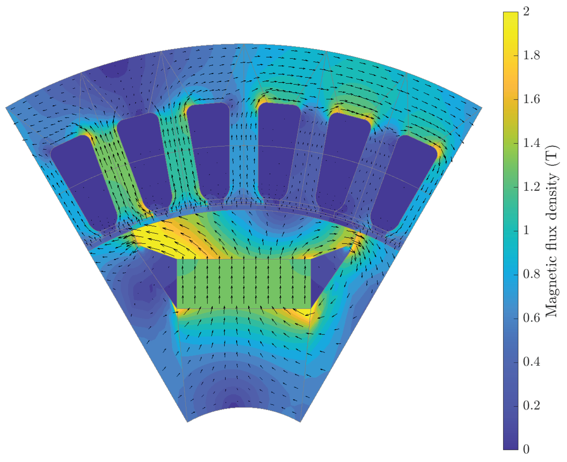
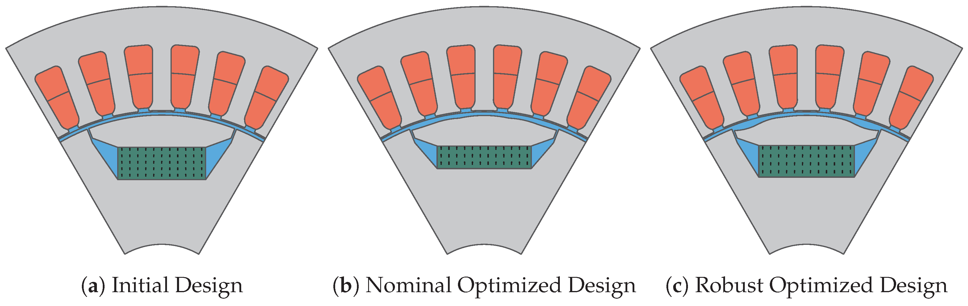
Our goal is to optimize the geometry of the rotor of an electric machine, as shown in Figure 1. In (7), the current density is $I_{\mathrm{app}}=9$ and the winding number $n_{\mathrm{wind}}=12$. The optimization variables $\mathit{p}$ are the electric phase angle and the geometric parameters, consisting of the width (MW), height (MH) and distance from the air gap (MAG) of the permanent magnet, as shown in Figure 1, as well as five control points located at the air gap. Uncertainties are considered in the application current $I_{\mathrm{app}}$, as well as in the radial offsets of the five optimized control points. The uncertainty set for the parameter $I_{\mathrm{app}}$ is one-dimensional and given by 5.5% of the nominal value 9. The uncertainty set for the control points is a five-dimensional sphere with radius $0.25 \mathrm{mm}$, which is 0.56% of the rotor radius. A summary of the starting point for the optimization and the bounds on the optimization variables can be found in

Table 1. Lengths in millimeters and angles in degrees are provided for the initial motor parameters and bounds for the optimization.

Parameter Name	Initial	Min	Max
Height of magnet (MH)	7	1.5	12
Width of magnet (MW)	19	7	23
Distance to air gap (MAG)	7	5	15
Operating angle	0	−10	10

. The parameters required to describe the geometry of the machine can be found in ([12], Figure A.1). The weights in the objective function are chosen as $m_1=3000$ and $m_2=130$ to balance the competing optimization goals. The torque is evaluated at discrete angles of rotation $\alpha \in \{0,1,\dots ,19\}$. The mean torque has the lower bound $T_{\mathrm{desired}}=1.55 \mathrm{Nm}$. The rotor is constructed from 12 distinct patches, and the stator shape is constructed from 79 patches. This results in a total of 160 control points that define the rotor’s shape, and another 669 control points that define the stator’s shape. We have in total 792 degrees of freedom for the rotor and 2783 for the stator. The magnetic flux density for the initial design is depcted in Figure 3. Figure 4a shows the initial design, Figure 4b the nominal optimized design for the optimization problem (12) and Figure 4c the robust optimized design that accounts for uncertainties in parameters and shape.

Starting from an initial magnet geometry with width $\mathrm{MW}=19 \mathrm{mm}$ and height $\mathrm{MH}=7 \mathrm{mm}$, the nominal optimization achieves a reduction in the magnet’s material usage by approximately 26%, while the desired average torque is maintained. In addition, the torque ripple is decreased by 96%, as seen also in Figure 5. The robust design, which optimizes the worst-case behavior and satisfies the constraints for all realizations of the uncertain quantities in the uncertainty set, still shows an improvement over the initial configuration. Here, a reduction in the magnet material by about 8% is achieved, as well as a torque ripple reduction of approximately 92% (see Figure 5). This is also represented in the values of the objective function, where the nominal optimization reaches a value of $0.766$ from initially $13.53$, whereas the robust optimization approach reaches a value of $1.464$. In addition, the robust optimization ensures the feasibility of the critical constraint, which is the lower bound on the average torque, for all realizations in the uncertainty set. On the other hand, if we compute the worst case of the average torque for the nominal optimized design over the uncertainty set, then it violates the lower bound, in contrast to the robust optimal design, as shown in

Table 2. Comparing the iteration numbers for the nominal and robust optimization.

Optimization Type	Iterations	Function Evaluations	Computation Time	Torque Avg. Worst Case at Optimal Design	Interval of Torque Ripple at Worst Case
Nominal Optimization	60 + 0	102 + 0	21 min	1.445 Nm	[1.42, 1.62]
Robust Optimization	55 + 123	184 + 221	1 h 19 min	1.561 Nm	[1.551, 1.568]

. This is because the nominal optimization problem (12) does not take uncertainties into account and chooses the area of the magnet to be too small, so that it does not achieve a sufficient average torque when uncertainties occur. However, the robust problem (18) resolves the uncertainties and accordingly selects a larger area of the magnet, achieving a sufficient average torque that is feasible even in the worst case. In summary, robust optimization can handle uncertainties and still achieve comparable performance.

For the nominal optimization problem, the computation is completed in about 21 min and requires 102 function evaluations. A comparison of the nominal optimization method with an evolutionary algorithm can be found in [9]. In [27], it is shown that the nominal optimization method can simultaneously reduce several objectives relevant to electric machines, such as the cost, torque ripple and losses, even with a large number of optimization variables.

The robust optimization requires 79 min for a similar number of iterations. This is primarily due to the iterative determination of worst-case scenarios, which results in an increased number of 405 function evaluations. However, as the optimization progresses, the number of iterations required to compute the worst case decreases. After only a few iterations, the number of iterations is quickly reduced, as observed in Figure 6. This is mainly for the following reason. During the outer loop, the optimization variables of the robust optimization problem (18) converge and thus also the solutions of the worst-case problems (17) converge. Since we start the solution of (17) in each iteration with the solution obtained in the previous outer iteration, we have already a good starting point and require only a few iterations to solve the worst-case problems (17). The fact that the robust problem is solved at about four times the cost of the nominal problem underlines the efficiency of the proposed approach. The details are summarized in Table 2 and

Table 3. Comparing the optimization objectives.

Optimization	Magnet Area	Torque Std	Objective Function Value	Mean Torque
Initial Setting	133.0 mm2	0.101 Nm	13.53	1.517 Nm
Nominal Optimization	98.08 mm2	0.0038 Nm	0.766	1.564 Nm
Robust Optimization	124.41 mm2	0.0084 Nm	1.464	1.563 Nm

.

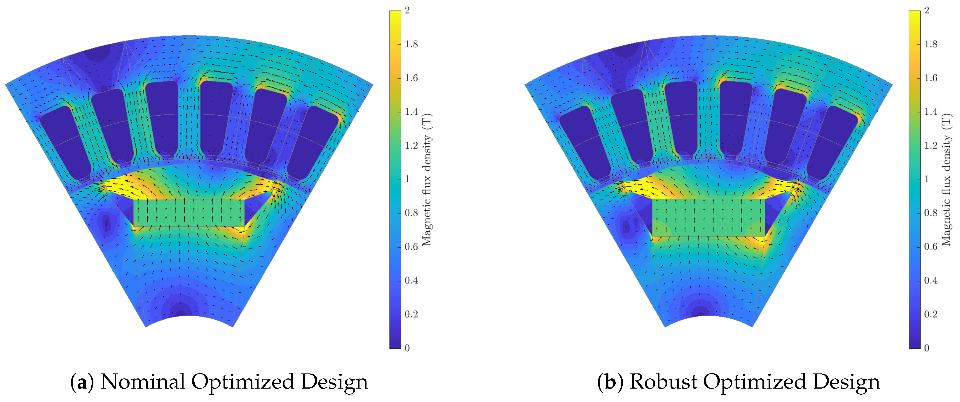
Since the current implementation is done in MATLAB^®, the code is not yet optimized for performance. Calculating the derivatives and solving the problem for different rotation angles is, for example, not yet parallelized. One limitation to note is that the calculations do not account for saturation (nonlinear material behavior), which is essential for accurate design. Therefore, we provide a comparison for the magnetic flux density for the optimized design and the robust optimized design in Figure 7. The magnetic flux density for the initial design is shown in Figure 3.

We focus next on the achieved reduction in the torque ripple. By applying free-shape optimization at the air gap by moving the control points, as shown in Figure 4b,c, we are able to reduce the torque ripple significantly. Figure 5 shows the torque profiles during nominal and robust optimization. In Figure 5a, a significant reduction in torque ripple is observed after only 20 iterations, similar to the results in [9]. In Figure 5b, we observe at iteration zero that the mean torque from the nominal design is initially insufficient for the robust design due to uncertainties in the optimal design. To address this, the mass of the magnet is increased to satisfy the torque requirements. This early adjustment phase is typical for robust optimization methods and highlights that solutions that are feasible under nominal conditions may not be as feasible under uncertainty. For the first iteration of the robust optimization, assuming the worst case for every parameter even yields torque ripples comparable to the initial design. After several iterations, the optimizer manages to reduce the torque again quite significantly, but not as much as the nominal optimization. Overall, both the nominal and robust optimization methods show a reduction in torque ripple within the first few iterations, which is also the main contributor to the rapid decrease in the objective function value.

5. Conclusions and Discussion

In this paper, we have proposed an algorithm for the robust optimization of complex PDE-constrained problems. We have applied the method to the combined shape and parameter optimization, with uncertainties incorporated in both. The underlying PDEs are discretized using IGA. This yields a precise representation of the geometry and provides a convenient framework for shape optimization. While the focus has been on the context of electric machine design, the principles and techniques employed are not limited to this application and can be applied to a wide range of robust optimal design problems. The additional costs for robust optimization are small compared to nominal optimization. In future research, we plan to extend the optimization framework to three-dimensional problems, including nonlinearity and hysteresis. Moreover, we plan to apply our methods to robust topology optimization.

References

- Gangl, P. Sensitivity-Based Topology and Shape Optimization with Application to Electrical Machines. Ph.D. Thesis, JKU Linz, Linz, Austria, 2016. [Google Scholar]
- Gangl, P.; Köthe, S.; Mellak, C.; Cesarano, A.; Mütze, A. Multi-objective free-form shape optimization of a synchronous reluctance machine. COMPEL— Int. J. Comput. Math. Electr. Electron. Eng. 2022, 41, 1849–1864. [Google Scholar] [CrossRef]
- Lass, O.; Ulbrich, S. Model order reduction techniques with a posteriori error control for nonlinear robust optimization governed by partial differential equations. SIAM J. Sci. Comput. 2017, 39, S112–S139. [Google Scholar] [CrossRef]
- Belahcen, A.; Martin, F.; Zaïm, M.E.H.; Dlala, E.; Kolondzovski, Z. Combined fe and particle swarm algorithm for optimization of high speed pm synchronous machine. COMPEL— Int. J. Comput. Math. Electr. Electron. Eng. 2015, 34, 475–484. [Google Scholar] [CrossRef]
- Gangl, P.; Langer, U.; Laurain, A.; Meftahi, H.; Sturm, K. Shape Optimization of an Electric Motor Subject to Nonlinear Magnetostatics. SIAM J. Sci. Comput. 2015, 37, B1002–B1025. [Google Scholar] [CrossRef]
- Choi, J.S.; Izui, K.; Nishiwaki, S.; Kawamoto, A.; Nomura, T. Rotor pole design of IPM motors for a sinusoidal air-gap flux density distribution. Struct. Multidiscip. Optim. 2012, 46, 445–455. [Google Scholar] [CrossRef]
- Kuci, E. Shape and Topology Optimization for Electro-Mechanical Energy Converters. Ph.D. Thesis, Université de Liège, Liège, France, 2018. [Google Scholar]
- Brun, O.; Chadebec, O.; Ferrouillat, P.; Niyonzima, I.; Siau, J.; Meunier, G.; Gerbaud, L.; Vi, F.; Le Floch, Y. Sensitivity analysis using the virtual work principle for 2-D magnetostatic problems. IEEE Trans. Magn. 2023, 59, 7000804. [Google Scholar] [CrossRef]
- Wiesheu, M.; Komann, T.; Merkel, M.; Schöps, S.; Ulbrich, S.; Cortes Garcia, I. Combined Parameter and Shape Optimization of Electric Machines with Isogeometric Analysis. arXiv 2023, arXiv:2311.06046. [Google Scholar] [CrossRef]
- Wang, Y.; Wang, Z.; Xia, Z.; Poh, L.H. Structural Design Optimization Using Isogeometric Analysis: A Comprehensive Review. CMES-Comput. Model. Eng. Sci. 2018, 117, 455–507. [Google Scholar] [CrossRef]
- Ben-Tal, A.; Goryashko, A.; Nemirovski, A. Robust Optimization; Princeton University Press: Princeton, NJ, USA, 2009. [Google Scholar]
- Bontinck, Z.; Corno, J.; Schöps, S.; De Gersem, H. Isogeometric analysis and harmonic stator-rotor coupling for simulating electric machines. Comput. Methods Appl. Mech. Eng. 2018, 334, 40–55. [Google Scholar] [CrossRef]
- Clarke, F.H. Generalized Gradients and Applications. Trans. Am. Math. Soc. 1975, 205, 247–262. [Google Scholar] [CrossRef]
- Bertsimas, D.; Nohadani, O.; Teo, K. Robust Nonconvex Optimization for Simulation-Based Problems. 2007. Available online: https://api.semanticscholar.org/CorpusID:9760047 (accessed on 12 April 2024).
- Hughes, T.J.R.; Cottrell, J.A.; Bazilevs, Y. Isogeometric analysis: CAD, finite elements, NURBS, exact geometry and mesh refinement. Comput. Methods Appl. Mech. Eng. 2005, 194, 4135–4195. [Google Scholar] [CrossRef]
- Piegl, L.; Tiller, W. The NURBS Book, 2nd ed.; Springer: Berlin, Germany, 1997. [Google Scholar]
- De Boor, C. On Calculating with B-splines. J. Approx. Theory 1972, 6, 50–62. [Google Scholar] [CrossRef]
- Da Veiga, L.; Buffa, A.; Sangalli, G.; Vázquez, R. Mathematical analysis of variational isogeometric methods. Acta Numer. 2014, 23, 157–287. [Google Scholar] [CrossRef]
- Pahner, U. A General Design Tool for Theoretical Optimization of Electromagnetic Energy Transducers. Ph.D. Thesis, KU Leuven, Leuven, Belgium, 1998. [Google Scholar]
- Buffa, A.; Vázquez, R.H.; Sangalli, G.; da Veiga, L.B. Approximation estimates for isogeometric spaces in multipatch geometries. Numer. Methods Partial. Differ. Equ. 2015, 31, 422–438. [Google Scholar] [CrossRef]
- Janssen, J. Extended Analytical Charge Modeling for Permanent-Magnet Based Devices: Practical Application to the Interactions in a Vibration Isolation System. Ph.D. Thesis, Electrical Engineering, Eindhoven University of Technology Library, Eindhoven, The Netherlands, 2011. [Google Scholar]
- Salon, S.J. Finite Element Analysis of Electrical Machines; Kluwer: New York, NY, USA, 1995. [Google Scholar]
- Sibley, M. Introduction to Electromagnetism: From Coulomb to Maxwell, 2nd ed.; CRC Press: Boca Raton, FL, USA, 2021. [Google Scholar] [CrossRef]
- Egger, H.; Harutyunyan, M.; Löscher, R.; Merkel, M.; Schöps, S. On torque computation in electric machine simulation by harmonic mortar methods. J. Math. Ind. 2022, 12, 6. [Google Scholar] [CrossRef]
- Binnemans, K.; Jones, P.T.; Blanpain, B.; Van Gerven, T.; Yang, Y.; Walton, A.; Buchert, M. Recycling of rare earths: A critical review. J. Clean. Prod. 2013, 51, 1–22. [Google Scholar] [CrossRef]
- Ehrgott, M. Multicriteria Optimization; Springer: Berlin, Germany, 2005. [Google Scholar]
- Wiesheu, M.; Komann, T.; Merkel, M.; Schöps, S.; Ulbrich, S.; Garcia, I.C. Spline-Based Rotor and Stator Optimization of a Permanent Magnet Synchronous Motor. arXiv 2024, arXiv:2402.19065. [Google Scholar] [CrossRef]
- Leyffer, S.; Menickelly, M.; Munson, T.; Vanaret, C.; Wild, S.M. A survey of nonlinear robust optimization. INFOR Inf. Syst. Oper. Res. 2020, 58, 342–373. [Google Scholar] [CrossRef]
- Wang, I.; Becker, C.; Van Parys, B.; Stellato, B. Learning for Robust Optimization. arXiv 2023, arXiv:2305.19225. [Google Scholar]
- Kolvenbach, P.; Lass, O.; Ulbrich, S. An approach for robust PDE-constrained optimization with application to shape optimization of electrical engines and of dynamic elastic structures under uncertainty. Optim. Eng. 2018, 19, 697–731. [Google Scholar] [CrossRef]
- Diehl, M.; Bock, H.G.; Kostina, E. An approximation technique for robust nonlinear optimization. Math. Program. 2006, 107, 213–230. [Google Scholar] [CrossRef]
- Zhang, Y. General robust-optimization formulation for nonlinear programming. J. Optim. Theory Appl. 2007, 132, 111–124. [Google Scholar] [CrossRef]
- Danskin, J.M. The Theory of Max-Min and Its Application to Weapons Allocation Problems; Springer: Berlin/Heidelberg, Germany, 1967. [Google Scholar] [CrossRef]
- Bertsimas, D.; Nohadani, O.; Teo, K.M. Nonconvex Robust Optimization for Problems with Constraints. INFORMS J. Comput. 2010, 22, 1–177. [Google Scholar] [CrossRef]
- Vázquez, R. A new design for the implementation of isogeometric analysis in Octave and Matlab: GeoPDEs 3.0. Comput. Math. Appl. 2016, 72, 523–554. [Google Scholar] [CrossRef]
- Curtis, F.E.; Mitchell, T.; Overton, M.L. A BFGS-SQP Method for Nonsmooth, Nonconvex, Constrained Optimization and its Evaluation using Relative Minimization Profiles. Optim. Methods Softw. 2017, 32, 148–181. [Google Scholar] [CrossRef]
- Tröltzsch, F. Optimal Control of Partial Differential Equations: Theory, Methods, and Applications; American Mathematical Society: New York, NY, USA, 2010; ISBN 9780821849040. [Google Scholar] [CrossRef]
- Qian, X. Full Analytical Sensitivities in NURBS Based Isogeometric Shape Optimization. Comput. Methods Appl. Mech. Eng. 2010, 199, 2059–2071. [Google Scholar] [CrossRef]
- Wall, W.; Frenzel, M.; Cyron, C. Isogeometric Structural Shape Optimization. Comput. Methods Appl. Mech. Eng. 2008, 197, 2976–2988. [Google Scholar] [CrossRef]
- Bader, B.W.; Kolda, T.G. Efficient MATLAB Computations with Sparse and Factored Tensors. SIAM J. Sci. Comput. 2007, 30, 205–231. [Google Scholar] [CrossRef]
- Monk, P. Finite Element Methods for Maxwell’s Equations; Oxford University Press: Oxford, UK, 2003. [Google Scholar]
Figure 1.
Geometry of of a PMSM constructed in MATLAB® 9.14.0 R2023a using IGA and the open-source package GeoPDEs.
Figure 2.
Geometry model of the PMSM with highlighted control points as described in (2) and patch boundaries. The model was originally based on [19].
Figure 3.
Plot of the solution to (9), representing the magnetic flux density.
Figure 4.
A visual representation of the optimization results: the initial design (a), the optimized design under nominal conditions (b) and the robust optimized design (c).
Figure 5.
Optimization history of the torque ripple for nominal optimization (a) and robust optimization (b). The nominal optimization and robust optimization show a significant reduction in the torque ripple at the end of the optimization.
Figure 6.
Number of iterations to determine the worst-case scenario during the robust optimization process. The number of needed iterations decreases with increasing optimization iterations.
Figure 7.
Resulting magnetic flux density of the the nominal design (a) and the robust design (b).