
A Two-Stage Method for Aerial Tracking in Adverse Weather Conditions

1
College of Science, Zhejiang University of Technology, Hangzhou 310023, China
2
School of Science, Zhejiang University of Science and Technology, Hangzhou 310023, China
*
Author to whom correspondence should be addressed.
Mathematics 2024, 12(8), 1216; https://doi.org/10.3390/math12081216
Submission received: 27 February 2024
/
Revised: 29 March 2024
/
Accepted: 4 April 2024
/
Published: 18 April 2024
(This article belongs to the Special Issue Applications of Artificial Intelligence, Machine Learning and Data Science)
Abstract
:To tackle the issue of aerial tracking failure in adverse weather conditions, we developed an innovative two-stage tracking method, which incorporates a lightweight image restoring model DADNet and an excellent pretrained tracker. Our method begins by restoring the degraded image, which yields a refined intermediate result. Then, the tracker capitalizes on this intermediate result to produce precise tracking bounding boxes. To expand the UAV123 dataset to various weather scenarios, we estimated the depth of the images in the dataset. Our method was tested on two famous trackers, and the experimental results highlighted the superiority of our method. The comparison experiment’s results also validated the dehazing effectiveness of our restoration model. Additionally, the components of our dehazing module were proven efficient through ablation studies.
1. Introduction
Visual object tracking (VOT) is an important research topic in the field of computer vision. Generally speaking, its task is to locate a moving target in a video sequence based on the initial frame given. The tracking task is becoming more challenging due to factors like variable appearance, occlusion, attraction from similar objects, fast movement of the target, etc.
In recent years, a large number of trackers have been proposed to solve this issue, ranging from the initial architectures based on the Siam Network: SiamFC [1], SiamRPN [2] and SiamFC++ [3]; to the architectures based on transformers: TransT [4], SwinT [5], OSTrack [6], and others [7,8,9]; and recent architectures based on temporal and spatial methods: TCTrack [10], STMTrack [11], STARK [12], and AIATrack [13]. These single-object trackers have demonstrated remarkable performance on various mainstream Single-Object Tracking (SOT) datasets, such as OTB [14], VOT [15], GOT10K [16], TrackingNet [17], LaSOT [18], UAV123 [19], etc. However, these benchmarks typically simulate general tracking scenarios, and existing trackers are also designed for such conditions. However, in reality, tracking environments are unpredictable and dynamic, and it has been observed that state-of-the-art trackers might not perform well in environments with strong weather disturbances.
The dataset UAV123 [19] encompasses a collection of low-altitude UAV-captured videos. It comprises 123 medium-to-long video sequences, which are typically used as the test set without additional training. Recent tracking algorithms have achieved very promising performance on this dataset, with OSTrack [6] achieving an AUC of 0.707, AIA [13] achieving an AUC of 0.706, and MixFormer [7] achieving an AUC of 0.704, etc. Nowadays, drones have been widely applied in various fields such as visual positioning, missile tracking, and anti-missile systems. Nevertheless, aerial tracking still faces some unresolved difficulties [20,21,22]; some of the most representative are motion blur and occlusion caused by adverse weather conditions.
In adverse weather, such as heavy rain or fog, a classic tracking system could lose target information due to the obstruction or interference caused by the rain and fog during the tracking process, which would result in erroneous tracking. To address this issue, we artificially added rain and haze to the UAV123 [19] and applied some state-of-the-art trackers [4,6] for testing. Figure 1 shows the result of OSTrack [6] on one frame of the UAV123 [19], and it is evident that in adverse weather, most tracking algorithms fail due to haze. Furthermore, the performance stays almost unaffected in rainy scenarios.
To solve the tracking problem in adverse weather conditions, we propose a novel method for tracking, and the method is mainly divided into two stages. The noisy image is fed into a light dehazing network to generate intermediate results and then sent into a tracking network to obtain the final tracking result. Recent studies show that researchers are focusing on end-to-end single-image defogging algorithms. These methods can be divided into two kinds. One is based on prior information [23,24,25,26], and the other is based on deep learning [27,28,29,30]. Since neural networks have become prevalent, researchers prefer letting the network autonomously learn parameters, as traditional methods with manually introduced prior information have limitations and lack the generalization ability of deep learning methods. Chen et al. [31] proposed a new end-to-end gated context aggregation network called GCANet for image dehazing, which is characterized by the use of smooth diffusion convolution to avoid grid artifacts and the fusion of features at different levels through gated sub-networks. Qin et al. [32] proposed a new feature fusion attention network called FFANet, which introduces both pixel attention and channel attention, enabling the entire network to perform well on images with dense fog and a rich texture. The application of the attention mechanism in the dehazing field has become increasingly widespread.
In our two-stage tracking method, a light pretrained image dehazing network called Dilated Attention Dehaze Network (DADNet) is proposed. Our DADNet is pretrained on the indoors of RESIDE [33]; it can obtain a proper intermediate result from a noisy input. In the second stage, the integrated tracker can predict final bounding boxes based on the intermediate results. We applied this two-stage tracking method to the complex field of aerial tracking and simulated five different adverse weather scenarios from light to dense fog referring to HazeRD [34] on the UAV123 [19], and the corresponding results indicated that our proposed two-stage tracking method can effectively perform tracking tasks under adverse weather scenarios.
We propose an attention module which is more powerful and faster in convergence than Qin’s method [32]. It is based on the dilated convolution called Dilated Attention. It has a larger receptive field to pay attention to the haze distribution of different pixels. To verify the effectiveness of dehazing, we trained the network on the dehazing benchmark RESIDE [33] and calculated the PSNR and SSIM compared with other dehazing networks. The experimental result showed that our proposed network is superior to them.
Generally speaking, our main works are summarized as follows:
- We propose a light end-to-end dehazing network called DADNet, which has a good removal effect on high-concentration and unevenly distributed fog. DADNet is fine-tuned to improve the object tracking that follows. Unlike standard image dehazing that aims for overall visual improvement, our method focuses specifically on tracking performance. We use Dilated Attention Blocks (DABs) to protect and highlight the image features that are important for reliable tracking. This focus ensures that our dehazing is a key part of the tracking algorithm, creating a beneficial relationship between the two stages. DADNet also performs better than other dehazing networks in the RESIDE [33] benchmark tests, proving its effectiveness in real-world scenarios.
- A novel two-stage tracking method is proposed to track targets under adverse weather conditions. It combines the light dehazing backbone DADNet with a SOTA tracker. We applied this method to UAV123 [19] with five different levels of fog density. The experimental results show that our two-stage tracking method can effectively solve the problem of tracking errors in adverse weather conditions.
- In order to further analyze the impact of rainy and foggy weather on tracking performance, we conducted experiments using several state-of-the-art trackers, and the experimental results showed that the performance of tracking was greatly affected by foggy weather.
2. Related Work
2.1. Rain Image Formation
Mathematically speaking, an image observed on a rainy day can be modeled as a linear superimposition of a clean background image and a rain streak layer , expressed as Equation (1):
From the above equation, it can be seen that to manually generate rainy day images, a clean background image and a rain streak mask are required. The clean background image can be sourced from the UAV123 [19] and the mask of rain streak can be obtained from Rain100L and Rain100H [36]. Similarly, the method of removing rain streaks from an image involves decomposing the input image O into a clean background image B and a rain streak layer which is an ill-posed problem because the number of unknowns to be recovered is twice that of the input unknowns [37]. However, this paper does not focus on rain streak removal, as the impact of heavy rain on state-of-the-art trackers is minimal, making such removal unnecessary. For a detailed result analysis, please refer to the experimental results with rain tracking below.
2.2. Monocular Depth Estimation Method
The main task of depth estimation is to determine the depth of each pixel in an image, a challenge that has been central to computer vision research since its early stages. As a fundamental computer vision task, depth estimation has significant applications in many higher-level fields, including 3D reconstruction [38], fog simulation [39], and autonomous driving [40]. Traditional depth estimation can be mainly divided into two directions: one is based on stereo depth estimation, and the other is based on monocular depth estimation. Stereo depth estimation utilizes the left and right RGB images captured by a camera for stereo matching, generates a disparity map, and, finally, calculates the depth of each pixel through some camera parameters. Common methods include [41,42]. In contrast, monocular depth estimation only estimates the depth of each pixel with a color image. This poses an ill-posed problem, as the same input image could correspond to multiple plausible depth interpretations. Researchers have explored various methods to address this issue: [43,44,45,46].
Godard et al. [46] proposed a self-supervised monocular depth estimation method which outperforms other state-of-the-art self-supervised methods both qualitatively and quantitatively on the KITTI benchmark [47]. Inspired by their work, we adopted their pretrained model named mono+stereo_1024 × 320 on KITTI [47] and used the monocular estimation method to generate depth maps for the UAV123 [19]. The details of the depth map can be seen in Figure 2.
2.3. Atmospheric Scattering Model
The scattering of particles in the atmosphere is the main cause of haze. Scenes in foggy weather, whether observed by the human eye or captured by a camera, always suffer from reduced contrast and visibility.
Mie scattering theory [48] is applicable for analyzing light propagation under hazy conditions when the particle size involved is significantly larger than the wavelength of the light in Figure 3. In this article, the hazing processing is formulated as Equation (2):
where and are the hazy image and haze-free background, A is the global atmospheric light, and is the medium transmission map. As Zhang et al. proposed in [34], we set the airlight to 0.76 and simulated fog under five different concentrations in UAV123 [19] using five sets of parameters in Figure 4. Detailed configurations of these parameters are provided in Table 1.
In most previous dehazing models, the transmission map or the atmospheric light A is first estimated, followed by the recovery of the final haze-free image . However, in real-world scenarios, both and A are unknown and difficult to estimate. Recently, more and more deep learning-based dehazing network architectures have been proposed. These networks utilize the local receptive field of CNN to automatically learn parameter weights on a large-scale dataset, avoiding the introduction of prior information manually. Ref. [27] proposed an end-to-end-based CNN and multi-scale network to predict intermediate transmission maps. However, in recent years, dehazing networks have become larger and larger in order to keep up with the SOTA, diverging from the actual intention of dehazing. In this article, our main task is to propose a two-stage tracking method to solve the tracking error problem under high haze conditions. This method encompasses two distinct phases: dehazing and tracking. This means that the dehazing network embedded within the method must not be too large to avoid adversely affecting the tracking performance.
2.4. Visual Aerial Tracking
In recent years, with the emergence of fields such as visual localization and target tracking, some researchers have begun to focus on the field of aerial tracking; as a result, an increasing number of state-of-the-art tracking algorithms have shown good performance on UAV123 [19]. The evolution of these algorithms ranges from the initial transformer-based tracking architectures [4,5,6,7] to the newer architectures incorporating both temporal and spatial information [10,11,12,13]. However, in the real world, aerial tracking often encounters harsh weather conditions such as rain and haze, especially at high altitudes. The appearance of rainy and foggy weather causes motion blur and occlusion in the photos taken by drones, resulting in a significant decrease in algorithms’ tracking performance. To address this issue, we propose a two-stage tracking method that integrates a dehazing backbone with SOTA trackers, aiming to mitigate tracking errors in dense haze conditions.
3. Method
In this section, we first introduce the process of expanding UAV123 [19] to adverse weather scenarios and the pipeline of the two-stage tracking method. The overview of our light Dilated Attention Dehazing Network called DADNet and its significant components is given subsequently. Finally, we describe the loss function used in the training process of DADNet.
3.1. Tracking Pipeline
All the details and the processes of the tracking architecture can be seen in Figure 5. To address the tracking error caused by harsh environments, we first drew on some previous methods and artificially synthesized UAV123 [19] images with rain and haze, and we further simulated tracking in rainy and foggy conditions. In order to address the problem of erroneous tracking caused by high-concentration haze, we propose a two-stage tracking method which combines a light DADNet backbone with SOTA trackers. Finally, we applied it to different haze levels of UAV123 [19] and improved tracking performance effectively. Detailed results are presented in the experimental section below.
As mentioned in Equation (1), synthesizing a dataset with rain artificially requires a clean background image and a rain streak mask ; then, they are superimposed linearly to obtain the final image. Yang et al. [36] provided the corresponding rain streak mask Rain100L and Rain100H, and we obtained the corresponding clean background images from the tracking benchmark UAV123 [19]. Consequently, we were able to create versions of the UAV123 dataset with light and heavy rain conditions.
The UAV123 [19] does not contain depth information, and its image sequences were all captured by monocular cameras. We used the self-supervised monocular depth estimation method proposed by Godard et al. [46] and applied a pretrained model named mono+stereo_1024 × 320 on KITTI [47] directly to predict the depth information of UAV123 [19]. Based on Equation (2)) and inspired by the method of fog simulation proposed by Zhang et al. [34], we set five groups of parameters to obtain five different concentrations of foggy UAV123. Please refer to Table 1 below for detailed parameter configurations.
After completing the dataset for rain and haze conditions in UAV123, we conducted tests using SOTA trackers and drew a conclusion: the effect of rain on aerial tracking is minimal, but the effect of haze is significant, and it will increase gradually with the concentration of haze. For a detailed analysis, please refer to the experimental section.
To address aerial tracking errors in adverse weather conditions, we propose a two-stage tracking method which is composed of a light dehazing backbone and an efficient tracker. In the first stage, we trained a light dehazing backbone to extract commendable intermediate results from the noisy input on the indoors of RESIDE [33], while in the second stage, pretrained SOTA trackers such as [4,6] were used to predict final bounding boxes based on the intermediate results. Finally, we tested our two-stage tracking method across five distinct levels of simulated foggy conditions. The experimental results demonstrate the effectiveness of our approach.
3.2. Overall Architecture of Our Model
In this section, we introduce the proposed DADNet, and its detailed structures are illustrated in Figure 6. Our network is designed as a light encoder–decoder architecture. In the encoder, the foggy image is first subjected to feature pre-extraction through three layers of convolutional layers, and Instance Norm and ReLU are applied immediately after each convolutional layer. Next, the obtained feature maps are sequentially processed by three groups of Dilated Attention Blocks (DABs) and residual blocks, with quantities , , and , respectively. It should be noted that the channel number C of the feature map will remain unchanged during this process in order to preserve semantic information during feature extraction. After passing three groups of dilated attention modules, the network can adaptively learn the haze distribution across the entire image, focusing more effectively on areas with dense haze.
The decoder’s architecture is efficiently designed to process the feature maps. It first adaptively learns from the three groups of feature maps generated in the encoder. These maps are then integrated through weighted summation, which fuses multi-scale feature information to produce the final feature map. This map undergoes further transformation into the haze-free image via a sequence of one deconvolution layer and two convolution layers, with each layer followed by Instance Norm.
3.3. Feature Attention
As [32] mentioned, most dehazing networks do not differentiate between channel information and pixel information, leading to challenges in handling images with uneven fog concentration distributions. To address this issue, Qin et al. [32] proposed a feature attention module, which mainly includes pixel attention and channel attention, making the entire network more flexible. Building on this foundation, we made improvements by adding batch normalization after both of the two convolutional layers which can be seen in Figure 7, further enhancing the dehazing performance and the convergence speed. For specific details, please refer to the ablation experiments below.
Channel attention (CA) primarily learns different type of channel information and eventually applies weighted processing to them. Initially, global average pooling is used to fuse the channel information for the input , transforming the shape of the feature map from C × H × W to C × 1 × 1. Following this, a 1 × 1 convolution operation is performed, accompanied by batch normalization. Finally, the output is passed through the activation function ReLU. This process can be summarized as follows:
In order to further extract information from the feature map, the intermediate results are processed through 1 × 1 convolutional operations, followed by corresponding batch normalization. Furthermore, the weight is finally output through the Sigmoid activation function. The entire process can be summarized as follows:
Finally, we multiply the weights and the input element-wise and obtain the final output of channel attention :
Pixel attention (PA) can focus more on local feature information mainly to solve the problem of uneven fog distribution.
Similar to CA, pixel attention first feeds the input into two convolutional layers with the corresponding activation functions ReLU and Sigmoid to gain the weight . It is worth noting that, in our approach, batch normalization is applied following the two convolutional layers. This process enhances the network’s stability and performance, and it can be described as follows:
Finally, we perform weighted processing by an element-wise multiplication of the input and the weights , resulting in the final output of pixel attention :
3.4. Dilated Attention Block
In the past, most visual tasks on the market tended to employ down-sampling to gradually merge feature information of different scales [51,52,53]. This allowed the final feature map to capture multi-scale information from the original image, which improved the model’s generalization ability and helped to avoid over-fitting. However, for certain pixel-level prediction tasks, there is a phenomenon of spatial resolution loss during the multi-scale feature extraction process through down-sampling. Inspired by the previous findings [31,54], we use dilated convolution. This method is designed to address the shortcomings of ordinary convolution receptive fields. By employing dilated convolution, we maintain a constant number of channels during feature extraction, avoiding down-sampling and, thereby, preventing the loss of spatial resolution.
Dilated convolution is different from regular convolution; it can be seen as a convolution with a dilated filter. In the one-dimensional case, given a one-dimensional input f and a convolution kernel of size k, the output of the corresponding dilated convolution can be described as follows:
where r represents dilation rate. In this way, it can increase the receptive field from k to .
In addition, we incorporate a convolutional layer with a kernel size of which shares weights across all channels, referring to [31,55], before dilated convolutions to avoid grid artifacts [31,56] caused by subsequent expansion convolutions. The entire process of implementing the dilated convolution can be described as follows:
where I and denote input and feature map, respectively; stands for Instance Norm. Furthermore, the above process is executed twice.
To endow the model with a global modeling capability, we add the attention module mentioned above after the dilated convolution and apply residual connections. This approach implicitly further amplifies the receptive fields of the dilated convolution, enabling the network to focus more effectively on the global distribution of haze. The specific process can be described as follows:
where denotes the feature map by dilated convolution; and stand for channel attention and pixel attention, respectively.
3.5. Multi-Scale Attention Block
Building on the approach outlined by Qin et al. (2020) [32], we process the data through three distinct DAB modules as previously described. Subsequently, we concatenate the feature maps derived from each set and apply feature attention mechanisms to derive adaptive learning weights effectively. Finally, we execute a weighted fusion of the three distinct sets of feature maps to synthesize the final feature map. The above processes are named as Multi-Scale Attention Bloack (MSAB), and this enables the entire network to assimilate feature information across various scales while striving to preserve semantic integrity.
3.6. Training Loss
In this section, we introduce our innovative loss function. Some previous deep learning-based dehazing methods [27,28,57] adopt L2 loss while others [32,58] adopt L1 loss. Unlike previous methods, we directly use the image dehazing metric SSIM as the loss evaluation criterion. However, considering that SSIM tends to increase during the training process, we finally took the opposite of SSIM and used it as the final loss function, which can be described as follows:
where represents the parameters of the whole network; and correspond to the output of the net and ground truths, respectively; and indicate the means of and ; , denote the standard deviation of and ; and represents the covariance of and .
It is important to emphasize that employing the Structural Similarity Index (SSIM) as the loss function is more advantageous than utilizing the L2 loss function. A specific quantitative analysis is presented in the detailed results of the ablation experiment.
4. Experiments
4.1. Implementation Details
Our rain and haze tracking was divided into two stages: firstly, the proposed dehazing network was trained on the dataset RESIDE [33]. Then, the trained dehazing network was embedded into the current SOTA tracking algorithm. By comparing the tracking performance, we verified the superiority of our new proposed tracker. For the dehazing network’s training, we maintained the input and output channels of each dilated attention block at 64. The configuration of dilated attention blocks was established as , , and for the three respective groups, with their dilation rates set to {2, 4, 6}, respectively. Following this, we set the dilation rate of the residual block after dilated attention as {1, 2, 4}, respectively. It should be noted that the whole network was trained in 100 epochs with the Adam optimizer. The initial learning rate was set at 0.005 and underwent a decennial reduction every 40 epochs. The entire training process was executed on an NVIDIA GeForce GTX RTX4090 with 24 GB of VRAM, where we configured the batch size to be 10. The hardware on which our DADNet was tested was an NVIDIA GeForce GTX2080Ti graphics card. To measure the FPS, we calculated it based on the processing time per frame. Specifically, the additional processing time per frame introduced by our DADNet was 2 ms (FPS = 500).
4.2. Evaluation Metrics
The efficacy of the object tracking algorithms was quantitatively assessed through metrics such as success and precision, which are contingent upon defined thresholds for overlap and location error.
4.2.1. Success Rate
The success rate (S) evaluates the overlap between the predicted bounding box () and the ground truth bounding box (). It is defined as follows:
where is the overlap threshold. This metric is threshold-dependent, with a higher score indicating a better tracking performance.
4.2.2. Precision
The precision (P) measures the accuracy of the tracker in terms of the distance between the center points of and . This metric is also threshold-dependent, and is defined as follows:
where represents the location error threshold, and are the x and y coordinates of the center points of and , respectively.
4.3. Evaluation on RESIDE
In this section, we trained the model on the Indoor subset of the dehazing benchmark RESIDE [33] and tested it on the corresponding test set. To measure the algorithm’s performance, we compared it with some other networks such as CAP [59], AOD-Net [60], DehazeNet [27], GFN [61], and GCANet [31]. The data clearly demonstrated that our proposed network not only held its ground against other established dehazing networks but also surpassed CANet [31] in PSNR by a notable margin of 1.48, showcasing its superior performance. In addition, we selected the common metrics SSIM and PSNR [33] for dehazing evaluation, and except for the results of our proposed dehazing network, all other results are from their respective papers (Table 2).
It is important to highlight that we did not benchmark our dehazing results against the current state-of-the-art (SOTA) methods; this decision stems from the fact that our application domain differs from those typically addressed by SOTA benchmarks.
The primary objective for the SOTA tasks is to climb the ranks through achieving heightened PSNR and SSIM scores. However, our innovative two-stage tracking method demands a more agile dehazing network. The current SOTA dehazing networks are excessively bulky and, thus, incompatible with our streamlined method. Our network’s advantage lies in its lightweight design, ensuring that it meets our specific needs while maintaining high performance.
4.4. Synthesis of the Datasets
To assess the efficacy of our novel two-stage tracking approach under rainy conditions, we selected the UAV123 dataset as the cornerstone for our evaluation, owing to its broad endorsement and prevalent application within the aerial tracking research sphere. The UAV123 dataset offers a rich compilation of low-altitude aerial footage, establishing itself as a quintessential benchmark for gauging the performance of tracking algorithms within authentic environments. Additionally, this dataset encompasses a spectrum of demanding scenarios, including occlusions, rapid movements, and scale variations, which furnishes a thorough platform to scrutinize the resilience and flexibility of our proposed method.
In our pursuit to emulate inclement weather conditions for robust testing, we ingeniously augmented the UAV123 dataset by overlaying synthetic rain streaks, thereby crafting two derivative datasets that depict scenarios of light and heavy rain. Concurrently, to simulate haze, we utilized the sophisticated HazeRD simulation tool, which is renowned for its precise modeling of haze-related scattering and attenuation effects, as per the atmospheric scattering model. This integration with HazeRD allowed us to generate a continuum of fog-affected environments, each distinguished by varying visibility constraints. This initiative to blend UAV123 with HazeRD’s simulations establishes a formidable testing bed, enabling us to meticulously gauge the performance of our two-stage tracking method across an array of weather conditions, from pristine to the severely hampered, and underscores its viability for deployment in real-world aerial tracking contexts.
4.5. The Impact of Rain on Tracking Performance
We artificially used existing rain steak marks to synthesize two datasets with light rain and heavy rain in UAV123. Figure 3 shows the original images and the synthesized images. Utilizing the synthesized datasets described above, we conducted performance evaluations employing state-of-the-art trackers.
Table 3 presents a comparative analysis of the OSTrack [6] and TransT [4] trackers’ performance on the original, light rain, and heavy rain datasets. The data in the table suggest that rainy conditions appear to have a negligible effect on the tracking efficacy of unmanned aerial vehicles. Specifically, for the OSTrack [6] tracker, the AUC decreased by 1.63 percentage points in heavy-rain conditions, while it only decreased by 0.05 percentage points in light-rain conditions. In the same way, for the TransT [4] tracker, the AUC decreased by 2.15 percentage points in heavy-rain conditions, while it only decreased by 0.24 percentage points in light-rain conditions. Consequently, our focus is on enhancing tracking performance in foggy scenarios, as rainy conditions have not shown a substantial impact warranting optimization.
4.6. The Impact of Haze on Tracking Performance
Similarly, we used our generated depth maps to artificially synthesize the UAV123 under five different levels of haze followed by [34], and detailed parameters are described in Table 1. Figure 4 displays the actual results of UAV123 [19] under the five different levels of haze.
Firstly, we evaluated the performance of the SOTA trackers such as OSTrack [6] and TransT [4] on five different concentrations of foggy UAV123. Furthermore, we assessed the efficacy of our innovative two-stage tracking method that combines DADNet with the associated tracker, using the same datasets. Detailed comparison results are presented in Table 4. It is not difficult to observe that tracking performance significantly decreases in a highly foggy environment. Specifically, for the OSTrack [6] tracker, we observe a significant 36.42% drop in AUC when operating in adverse weather conditions. Similarly, the performance of the TransT [4] tracker is notably affected, with a 29.94% decrease in AUC in these challenging visibility scenarios. Furthermore, it is clear that our proposed network architecture demonstrably alleviates the adverse effects of such environmental factors.
4.7. The Comparison of Rain and Fog
Through experiments, we found that rain has less impact on object tracking than fog. Furthermore, it can be further explained from a mathematical perspective in this article that the hazing processing and raining are formulated as Equations (1) and (2).
In real life, the R in Equation (2) is usually quite sparse, and the impact of rain on images is mainly reflected in the local gradient distribution rather than in the color distribution. Therefore, rain does not affect the image in its entirety. Simultaneously, the main operations in the convolutional neural networks are the cross-correlation computations of convolutional layers and average pooling, which can reduce the effect of local gradient distribution interference on target feature extraction. So, in general, the tracking algorithm is relatively less disturbed by rain.
Furthermore, in Equation (2), we can see that each pixel of the original images is subjected to a weighted average operation with the global light intensity. Furthermore, owing to the intrinsic characteristics of fog, the transmittance of the medium decreases as the depth value of the pixel point increases, that is, as objects become farther from the camera. Consequently, the extent to which the image is influenced intensifies. Hence, foggy conditions can markedly diminish the sharpness and contrast of an image, leading to widespread blurring and a reduction in contrast levels. However, global blurring and diminished contrast within an image can substantially affect the performance of a convolutional neural network. This is due to the fact that such alterations directly disrupt the CNN’s foundational mechanisms for feature extraction and decision-making processes in classification tasks.
From a mathematical standpoint, blurring leads to the edges and texture details in an image becoming less defined, which, in turn, diminishes the convolutional layer’s capacity to extract features via the process of weighted summation. The reduction in contrast narrows the spectrum of pixel values, thereby limiting the dynamic scope of activation function outputs. This limitation reduces the network’s ability in identifying key features. The forfeiture of such detailed information becomes especially critical at the network’s deeper levels, significantly impairing its object recognition capabilities. Furthermore, the deterioration in image quality may also interfere with the optimization process, leading to issues such as vanishing or exploding gradients, which can make the training process more challenging.
4.8. The effDilated Attention Block
Quantitative data show that our two-stage tracking frame improved OSTrack [6] with 8.79% of AUC and 13.25% of precision in adverse weather. It also improved TransT [4] with 3.12% of AUC and 6.04% of precision in thick fog. To enhance the persuasiveness and conciseness of our results, we graphically represented the tracking performance of two trackers across various scenarios. For detailed insights, please refer to Figure 9.
Evidenced by the graphical data, our proposed tracking method exhibits a significant improvement over the original tracker, particularly under high-concentration haze conditions, indicating robustness at different levels of haze. It is worth mentioning that while applying our two-stage tracking method to the original UAV123 dataset, there may be a slight and often negligible deviation in performance. This is attributed to the two-stage nature of our tracking approach, as opposed to a seamless end-to-end process. However, the excellent performance improvement in high fog conditions will compensate for the slight performance decrease on original images.
Therefore, the addition of the Dilated Attention Block further enhances the effectiveness of the dehazing network, making it more efficient and converge faster when dealing with high-concentration fog, thus contributing significantly to the overall tracking performance. Compared to Qin’s method, the Dilated Attention Block is able to capture key features in the image more efficiently and adapt to different foggy environments faster by combining dilated convolution and attention mechanisms. As a result, our two-stage tracking method not only demonstrates superior performance in high-concentration foggy environments but also further improves the efficiency and accuracy of the dehazing network through the application of the Dilated Attention Block.
4.9. Ablation Study and Analysis
To further demonstrate the effectiveness of our proposed dehazing network, we conducted ablation experiments on different modules of the network, including the following: (1) with/without attention in dilated convolutions block; (2) with/without normalization in CA and PA; (3) using L2 loss or SSIM loss.
To conduct the ablation experiments mentioned above, we configured four different network architectures by gradually adding each module to the initial network. The experimental results are shown in Table 5. It is evident that the dehazing performance continued to improve in tandem with the progressive refinement of the network architecture. From the data in the table, it can be seen that using attention in dilated convolution yielded a gain of about 0.29 in PSNR; adding normalization in CA and PA further improved PSNR by about 0.39. Finally, using the SSIM loss function instead of the regular loss function also improved PSNR by about 0.4. Obviously, all the components of our network demonstrated positive effects.
5. Conclusions and Future Research
In this paper, we propose a two-stage aerial tracking method under adverse weather conditions. Specifically, we introduce a lightweight dehazing network called DADNet. DADNet is a lightweight network designed for image restoration, utilizing an encoder–decoder structure. In the encoder part, DADNet processes the image through successive layers to distill features and then employs Dilated Attention Blocks (DABs) to concentrate on regions shrouded in dense haze, enhancing the tracking accuracy. In the decoder part, it combines these features to create a clear, restored image. This network is effective in learning the distribution of haze in images and efficiently removing them. Then, we construct a two-stage tracking method that combines the proposed DADNet with state-of-the-art trackers. Additionally, we expanded the UAV123 dataset to include scenarios with rain and haze and applied our method to this expanded dataset. It is easily observed that haze can significantly impair the accuracy of tracking methods. The results of the comparison experiments demonstrated the effectiveness of our two-stage method.
In future research, we aim to broaden and refine our two-stage tracking strategy through a series of initiatives. We plan to encompass a wider array of weather conditions, including snow and sandstorms, to thoroughly evaluate the robustness of our method.
Author Contributions
Conceptualization, Y.F.; software, X.X.; validation, N.C.; writing—original draft, Q.S.; project administration, Y.F.; funding acquisition, L.Z. All authors have read and agreed to the published version of the manuscript.
Funding
This work was supported in part by the Natural Science Foundation of Zhejiang Province under Grant No. LGG21F030011, the Zhejiang Provincial Natural Science Foundation of China under Grant No. LQ24A010023, and the special Fundamental Research Funds for Zhejiang University of Science and Technology under Grant No. 2023QN055.
Data Availability Statement
The dataset UAV123 utilized in this study is openly available for research purposes. You can access the data in UAV123 at [http://doi.org/10.1007/978-3-319-46448-0_27], with the reference number [19].
Conflicts of Interest
The authors declare no conflict of interest.
References
- He, A.; Luo, C.; Tian, X.; Zeng, W. A twofold siamese network for real-time object tracking. In Proceedings of the IEEE Conference on Computer Vision and Pattern Recognition, Salt Lake City, UT, USA, 18–23 June 2018; pp. 4834–4843. [Google Scholar]
- Li, B.; Yan, J.; Wu, W.; Zhu, Z.; Hu, X. High performance visual tracking with siamese region proposal network. In Proceedings of the IEEE Conference on Computer Vision and Pattern Recognition, Salt Lake City, UT, USA, 18–23 June 2018; pp. 8971–8980. [Google Scholar]
- Xu, Y.; Wang, Z.; Li, Z.; Yuan, Y.; Yu, G. Siamfc++: Towards robust and accurate visual tracking with target estimation guidelines. In Proceedings of the AAAI Conference on Artificial Intelligence, New York, NY, USA, 7–12 February 2020; Volume 34, pp. 12549–12556. [Google Scholar]
- Chen, X.; Yan, B.; Zhu, J.; Wang, D.; Yang, X.; Lu, H. Transformer tracking. In Proceedings of the IEEE/CVF Conference on Computer Vision and Pattern Recognition, Nashville, TN, USA, 20–25 June 2021; pp. 8126–8135. [Google Scholar]
- Lin, L.; Fan, H.; Zhang, Z.; Xu, Y.; Ling, H. Swintrack: A simple and strong baseline for transformer tracking. Adv. Neural Inf. Process. Syst. 2022, 35, 16743–16754. [Google Scholar]
- Ye, B.; Chang, H.; Ma, B.; Shan, S.; Chen, X. Joint feature learning and relation modeling for tracking: A one-stream framework. In Proceedings of the European Conference on Computer Vision, Tel Aviv, Israel, 23–27 October 2022; Springer: Berlin/Heidelberg, Germany, 2022; pp. 341–357. [Google Scholar]
- Cui, Y.; Jiang, C.; Wang, L.; Wu, G. Mixformer: End-to-end tracking with iterative mixed attention. In Proceedings of the IEEE/CVF Conference on Computer Vision and Pattern Recognition, New Orleans, LA, USA, 18–24 June 2022; pp. 13608–13618. [Google Scholar]
- Sun, Z.; Liu, C.; Qu, H.; Xie, G. A novel effective vehicle detection method based on swin transformer in hazy scenes. Mathematics 2022, 10, 2199. [Google Scholar] [CrossRef]
- Li, D.; Chai, H.; Wei, Q.; Zhang, Y.; Xiao, Y. PACR: Pixel Attention in Classification and Regression for Visual Object Tracking. Mathematics 2023, 11, 1406. [Google Scholar] [CrossRef]
- Cao, Z.; Huang, Z.; Pan, L.; Zhang, S.; Liu, Z.; Fu, C. TCTrack: Temporal contexts for aerial tracking. In Proceedings of the IEEE/CVF Conference on Computer Vision and Pattern Recognition, New Orleans, LA, USA, 18–24 June 2022; pp. 14798–14808. [Google Scholar]
- Fu, Z.; Liu, Q.; Fu, Z.; Wang, Y. Stmtrack: Template-free visual tracking with space-time memory networks. In Proceedings of the IEEE/CVF Conference on Computer Vision and Pattern Recognition, Nashville, TN, USA, 20–25 June 2021; pp. 13774–13783. [Google Scholar]
- Yan, B.; Peng, H.; Fu, J.; Wang, D.; Lu, H. Learning spatio-temporal transformer for visual tracking. In Proceedings of the IEEE/CVF International Conference on Computer Vision, Montreal, BC, Canada, 11–17 October 2021; pp. 10448–10457. [Google Scholar]
- Gao, S.; Zhou, C.; Ma, C.; Wang, X.; Yuan, J. Aiatrack: Attention in attention for transformer visual tracking. In Proceedings of the European Conference on Computer Vision, Tel Aviv, Israel, 23–27 October 2022; Springer: Berlin/Heidelberg, Germany, 2022; pp. 146–164. [Google Scholar]
- Wu, Y.; Lim, J.; Yang, M.H. Online object tracking: A benchmark. In Proceedings of the IEEE Conference on Computer Vision and Pattern Recognition, Portland, OR, USA, 23–28 June 2013; pp. 2411–2418. [Google Scholar]
- Kristan, M.; Matas, J.; Leonardis, A.; Felsberg, M.; Cehovin, L.; Fernandez, G.; Vojir, T.; Hager, G.; Nebehay, G.; Pflugfelder, R. The visual object tracking vot2015 challenge results. In Proceedings of the IEEE International Conference on Computer Vision Workshops, Washington, DC, USA, 7–13 December 2015; pp. 1–23. [Google Scholar]
- Huang, L.; Zhao, X.; Huang, K. GOT-10k: A Large High-Diversity Benchmark for Generic Object Tracking in the Wild. IEEE Trans. Pattern Anal. Mach. Intell. 2019, 1562–1577. [Google Scholar] [CrossRef]
- Muller, M.; Bibi, A.; Giancola, S.; Alsubaihi, S.; Ghanem, B. Trackingnet: A large-scale dataset and benchmark for object tracking in the wild. In Proceedings of the European Conference on Computer Vision (ECCV), Munich, Germany, 8–14 September 2018; pp. 300–317. [Google Scholar]
- Fan, H.; Lin, L.; Yang, F.; Chu, P.; Deng, G.; Yu, S.; Bai, H.; Xu, Y.; Liao, C.; Ling, H. Lasot: A high-quality benchmark for large-scale single object tracking. In Proceedings of the IEEE/CVF Conference on Computer Vision and Pattern Recognition, Long Beach, CA, USA, 15–20 June 2019; pp. 5374–5383. [Google Scholar]
- Mueller, M.; Smith, N.; Ghanem, B. A benchmark and simulator for uav tracking. In Proceedings of the Computer Vision–ECCV 2016: 14th European Conference, Amsterdam, The Netherlands, 11–14 October 2016; Proceedings, Part I 14; Springer: Berlin/Heidelberg, Germany, 2016; pp. 445–461. [Google Scholar]
- Song, H.; Wang, R. Underwater image enhancement based on multi-scale fusion and global stretching of dual-model. Mathematics 2021, 9, 595. [Google Scholar] [CrossRef]
- Hu, M.; Li, Y.; Fan, J.; Jing, B. Joint Semantic Deep Learning Algorithm for Object Detection under Foggy Road Conditions. Mathematics 2022, 10, 4526. [Google Scholar] [CrossRef]
- Benaddy, A.; Labbadi, M.; Boubaker, S.; Alsubaei, F.S.; Bouzi, M. Predefined-Time Fractional-Order Tracking Control for UAVs with Perturbation. Mathematics 2023, 11, 4886. [Google Scholar] [CrossRef]
- Ancuti, C.; Ancuti, C.O.; De Vleeschouwer, C.; Bovik, A.C. Night-time dehazing by fusion. In Proceedings of the 2016 IEEE International Conference on Image Processing (ICIP), Phoenix, AZ, USA, 25–28 September 2016; pp. 2256–2260. [Google Scholar]
- Ancuti, C.O.; Ancuti, C.; Hermans, C.; Bekaert, P. A fast semi-inverse approach to detect and remove the haze from a single image. In Proceedings of the Asian Conference on Computer Vision, Queenstown, New Zealand, 8–12 November 2010; Springer: Berlin/Heidelberg, Germany, 2010; pp. 501–514. [Google Scholar]
- He, K.; Sun, J.; Tang, X. Single image haze removal using dark channel prior. IEEE Trans. Pattern Anal. Mach. Intell. 2010, 33, 2341–2353. [Google Scholar] [PubMed]
- Meng, G.; Wang, Y.; Duan, J.; Xiang, S.; Pan, C. Efficient image dehazing with boundary constraint and contextual regularization. In Proceedings of the IEEE International Conference on Computer Vision, Sydney, Australia, 1–8 December 2013; pp. 617–624. [Google Scholar]
- Cai, B.; Xu, X.; Jia, K.; Qing, C.; Tao, D. Dehazenet: An end-to-end system for single image haze removal. IEEE Trans. Image Process. 2016, 25, 5187–5198. [Google Scholar] [CrossRef]
- Ren, W.; Liu, S.; Zhang, H.; Pan, J.; Cao, X.; Yang, M.H. Single image dehazing via multi-scale convolutional neural networks. In Proceedings of the Computer Vision–ECCV 2016: 14th European Conference, Amsterdam, The Netherlands, 11–14 October 2016; Proceedings, Part II 14; Springer: Berlin/Heidelberg, Germany, 2016; pp. 154–169. [Google Scholar]
- Yang, X.; Xu, Z.; Luo, J. Towards perceptual image dehazing by physics-based disentanglement and adversarial training. In Proceedings of the AAAI Conference on Artificial Intelligence, New Orleans, LA, USA, 2–7 February 2018; Volume 32. [Google Scholar]
- Zhang, H.; Sindagi, V.; Patel, V.M. Joint transmission map estimation and dehazing using deep networks. IEEE Trans. Circuits Syst. Video Technol. 2019, 30, 1975–1986. [Google Scholar] [CrossRef]
- Chen, D.; He, M.; Fan, Q.; Liao, J.; Zhang, L.; Hou, D.; Yuan, L.; Hua, G. Gated context aggregation network for image dehazing and deraining. In Proceedings of the 2019 IEEE Winter Conference on Applications of Computer Vision (WACV), Waikoloa Village, HI, USA, 7–11 January 2019; pp. 1375–1383. [Google Scholar]
- Qin, X.; Wang, Z.; Bai, Y.; Xie, X.; Jia, H. FFA-Net: Feature fusion attention network for single image dehazing. In Proceedings of the AAAI Conference on Artificial Intelligence, New York, NY, USA, 7–12 February 2020; Volume 34, pp. 11908–11915. [Google Scholar]
- Li, B.; Ren, W.; Fu, D.; Tao, D.; Feng, D.; Zeng, W.; Wang, Z. Benchmarking single-image dehazing and beyond. IEEE Trans. Image Process. 2018, 28, 492–505. [Google Scholar] [CrossRef] [PubMed]
- Zhang, Y.; Ding, L.; Sharma, G. Hazerd: An outdoor scene dataset and benchmark for single image dehazing. In Proceedings of the 2017 IEEE International Conference on Image Processing (ICIP), Beijing, China, 17–20 September 2017; pp. 3205–3209. [Google Scholar]
- Han, J.; Li, W.; Fang, P.; Sun, C.; Hong, J.; Armin, M.A.; Petersson, L.; Li, H. Blind image decomposition. In Proceedings of the European Conference on Computer Vision, Tel Aviv, Israel, 23–27 October 2022; Springer: Berlin/Heidelberg, Germany, 2022; pp. 218–237. [Google Scholar]
- Yang, W.; Tan, R.T.; Feng, J.; Liu, J.; Guo, Z.; Yan, S. Deep joint rain detection and removal from a single image. In Proceedings of the IEEE Conference on Computer Vision and Pattern Recognition, Honolulu, HI, USA, 21–26 July 2017; pp. 1357–1366. [Google Scholar]
- Li, Y.; Tan, R.T.; Guo, X.; Lu, J.; Brown, M.S. Rain streak removal using layer priors. In Proceedings of the IEEE Conference on Computer Vision and Pattern Recognition, Las Vegas, NV, USA, 26 June–1 July 2016; pp. 2736–2744. [Google Scholar]
- Liu, H.; Tang, X.; Shen, S. Depth-map completion for large indoor scene reconstruction. Pattern Recognit. 2020, 99, 107112. [Google Scholar] [CrossRef]
- Sakaridis, C.; Dai, D.; Van Gool, L. Semantic foggy scene understanding with synthetic data. Int. J. Comput. Vis. 2018, 126, 973–992. [Google Scholar] [CrossRef]
- Ding, M.; Huo, Y.; Yi, H.; Wang, Z.; Shi, J.; Lu, Z.; Luo, P. Learning depth-guided convolutions for monocular 3d object detection. In Proceedings of the IEEE/CVF Conference on Computer Vision and Pattern Recognition Workshops, Seattle, WA, USA, 13–19 June 2020; pp. 1000–1001. [Google Scholar]
- Liang, Z.; Feng, Y.; Guo, Y.; Liu, H.; Chen, W.; Qiao, L.; Zhou, L.; Zhang, J. Learning for disparity estimation through feature constancy. In Proceedings of the IEEE Conference on Computer Vision and Pattern Recognition, Salt Lake City, UT, USA, 18–23 June 2018; pp. 2811–2820. [Google Scholar]
- Zhang, J.; Skinner, K.A.; Vasudevan, R.; Johnson-Roberson, M. Dispsegnet: Leveraging semantics for end-to-end learning of disparity estimation from stereo imagery. IEEE Robot. Autom. Lett. 2019, 4, 1162–1169. [Google Scholar] [CrossRef]
- Eigen, D.; Puhrsch, C.; Fergus, R. Depth map prediction from a single image using a multi-scale deep network. Adv. Neural Inf. Process. Syst. 2014, 27. [Google Scholar]
- Fu, H.; Gong, M.; Wang, C.; Batmanghelich, K.; Tao, D. Deep ordinal regression network for monocular depth estimation. In Proceedings of the IEEE Conference on Computer Vision and Pattern Recognition, Salt Lake City, UT, USA, 18–23 June 2018; pp. 2002–2011. [Google Scholar]
- Laina, I.; Rupprecht, C.; Belagiannis, V.; Tombari, F.; Navab, N. Deeper depth prediction with fully convolutional residual networks. In Proceedings of the 2016 Fourth International Conference on 3D Vision (3DV), Stanford, CA, USA, 25–28 October 2016; pp. 239–248. [Google Scholar]
- Godard, C.; Mac Aodha, O.; Firman, M.; Brostow, G.J. Digging into self-supervised monocular depth estimation. In Proceedings of the IEEE/CVF International Conference on Computer Vision, Seoul, Republic of Korea, 27 October–2 November 2019; pp. 3828–3838. [Google Scholar]
- Geiger, A.; Lenz, P.; Stiller, C.; Urtasun, R. Vision meets robotics: The kitti dataset. Int. J. Robot. Res. 2013, 32, 1231–1237. [Google Scholar] [CrossRef]
- McCartney, E.J. Optics of the atmosphere: Scattering by molecules and particles. IEEE J. Quantum Electron. 1976, 14, 698–699. [Google Scholar] [CrossRef]
- Fan, Q.; Chen, D.; Yuan, L.; Hua, G.; Yu, N.; Chen, B. Decouple learning for parameterized image operators. In Proceedings of the European Conference on Computer Vision (ECCV), Munich, Germany, 8–14 September 2018; pp. 442–458. [Google Scholar]
- Fan, Q.; Yang, J.; Hua, G.; Chen, B.; Wipf, D. A generic deep architecture for single image reflection removal and image smoothing. In Proceedings of the IEEE International Conference on Computer Vision, Venice, Italy, 22–29 October 2017; pp. 3238–3247. [Google Scholar]
- Liu, Z.; Xiao, B.; Alrabeiah, M.; Wang, K.; Chen, J. Generic model-agnostic convolutional neural network for single image dehazing. arXiv 2018, arXiv:1810.02862. [Google Scholar] [CrossRef]
- He, K.; Zhang, X.; Ren, S.; Sun, J. Deep residual learning for image recognition. In Proceedings of the IEEE Conference on Computer Vision and Pattern Recognition, Las Vegas, NV, USA, 26 June–1 July 2016; pp. 770–778. [Google Scholar]
- Szegedy, C.; Liu, W.; Jia, Y.; Sermanet, P.; Reed, S.; Anguelov, D.; Erhan, D.; Vanhoucke, V.; Rabinovich, A. Going deeper with convolutions. In Proceedings of the IEEE Conference on Computer Vision and Pattern Recognition, Boston, MA, USA, 7–12 June 2015; pp. 1–9. [Google Scholar]
- Yu, F.; Koltun, V. Multi-scale context aggregation by dilated convolutions. arXiv 2015, arXiv:1511.07122. [Google Scholar]
- Wang, Z.; Ji, S. Smoothed dilated convolutions for improved dense prediction. In Proceedings of the 24th ACM SIGKDD International Conference on Knowledge Discovery & Data Mining, New York, NY, USA, 19–23 August 2018; pp. 2486–2495. [Google Scholar]
- Hamaguchi, R.; Fujita, A.; Nemoto, K.; Imaizumi, T.; Hikosaka, S. Effective use of dilated convolutions for segmenting small object instances in remote sensing imagery. In Proceedings of the 2018 IEEE Winter Conference on Applications of Computer Vision (WACV), Lake Tahoe, NV, USA, 12–15 March 2018; pp. 1442–1450. [Google Scholar]
- Li, B.; Peng, X.; Wang, Z.; Xu, J.; Feng, D. Aod-net: All-in-one dehazing network. In Proceedings of the IEEE International Conference on Computer Vision, Venice, Italy, 22–29 October 2017; pp. 4770–4778. [Google Scholar]
- Lim, B.; Son, S.; Kim, H.; Nah, S.; Mu Lee, K. Enhanced deep residual networks for single image super-resolution. In Proceedings of the IEEE Conference on Computer Vision and Pattern Recognition Workshops, Honolulu, HI, USA, 21–26 July 2017; pp. 136–144. [Google Scholar]
- Zhu, Q.; Mai, J.; Shao, L. A fast single image haze removal algorithm using color attenuation prior. IEEE Trans. Image Process. 2015, 24, 3522–3533. [Google Scholar]
- Li, B.; Peng, X.; Wang, Z.; Xu, J.; Feng, D. An all-in-one network for dehazing and beyond. arXiv 2017, arXiv:1707.06543. [Google Scholar]
- Ren, W.; Ma, L.; Zhang, J.; Pan, J.; Cao, X.; Liu, W.; Yang, M.H. Gated fusion network for single image dehazing. In Proceedings of the IEEE Conference on Computer Vision and Pattern Recognition, Salt Lake City, UT, USA, 18–22 June 2018; pp. 3253–3261. [Google Scholar]
- Chen, C.; Do, M.N.; Wang, J. Robust image and video dehazing with visual artifact suppression via gradient residual minimization. In Proceedings of the Computer Vision–ECCV 2016: 14th European Conference, Amsterdam, The Netherlands, 11–14 October 2016; Proceedings, Part II 14; Springer: Berlin/Heidelberg, Germany, 2016; pp. 576–591. [Google Scholar]
Figure 1.
Different trackers’ actual tracking performance on UAV123 [19] with rain and fog. (a) The origin input. (b) The tracking result of our method and comparison method, it can be seen that in adverse weather, trackers would probably fail. (c) This denotes that the rainy weather has limited impact on the tracking result.

Figure 2.
(a) The images comes from UAV123 [19], which itself does not contain depth information. (b) We adopted a monocular depth estimation method called monodepth2 [46], which was proposed by previous researchers, to generate the corresponding depth information.

Figure 3.
Two rain streak layers named Rain100L and Rain100H which originated from [36] were linearly combined with the original image to generate the final UAV123 with light rain and heavy rain. Furthermore, only a portion of the synthesized UAV123 images with rain are shown in the figure.
Figure 3.
Two rain streak layers named Rain100L and Rain100H which originated from [36] were linearly combined with the original image to generate the final UAV123 with light rain and heavy rain. Furthermore, only a portion of the synthesized UAV123 images with rain are shown in the figure.

Figure 4.
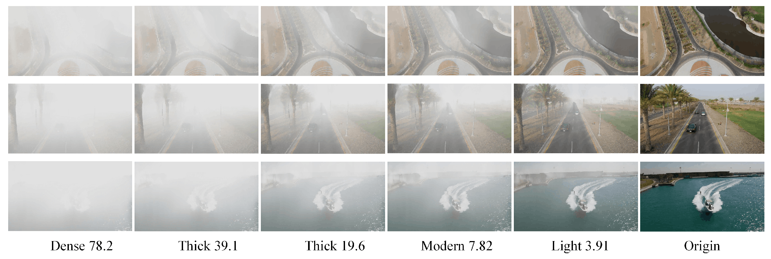
Based on the generated depth map, five different sets of parameters were used in the atmospheric model following [34] to simulate fog interference at five different concentrations in UAV123 [19]. Furthermore, only a portion of the synthesized UAV123 [19] images with haze are shown in the figure.
Figure 4.
Based on the generated depth map, five different sets of parameters were used in the atmospheric model following [34] to simulate fog interference at five different concentrations in UAV123 [19]. Furthermore, only a portion of the synthesized UAV123 [19] images with haze are shown in the figure.

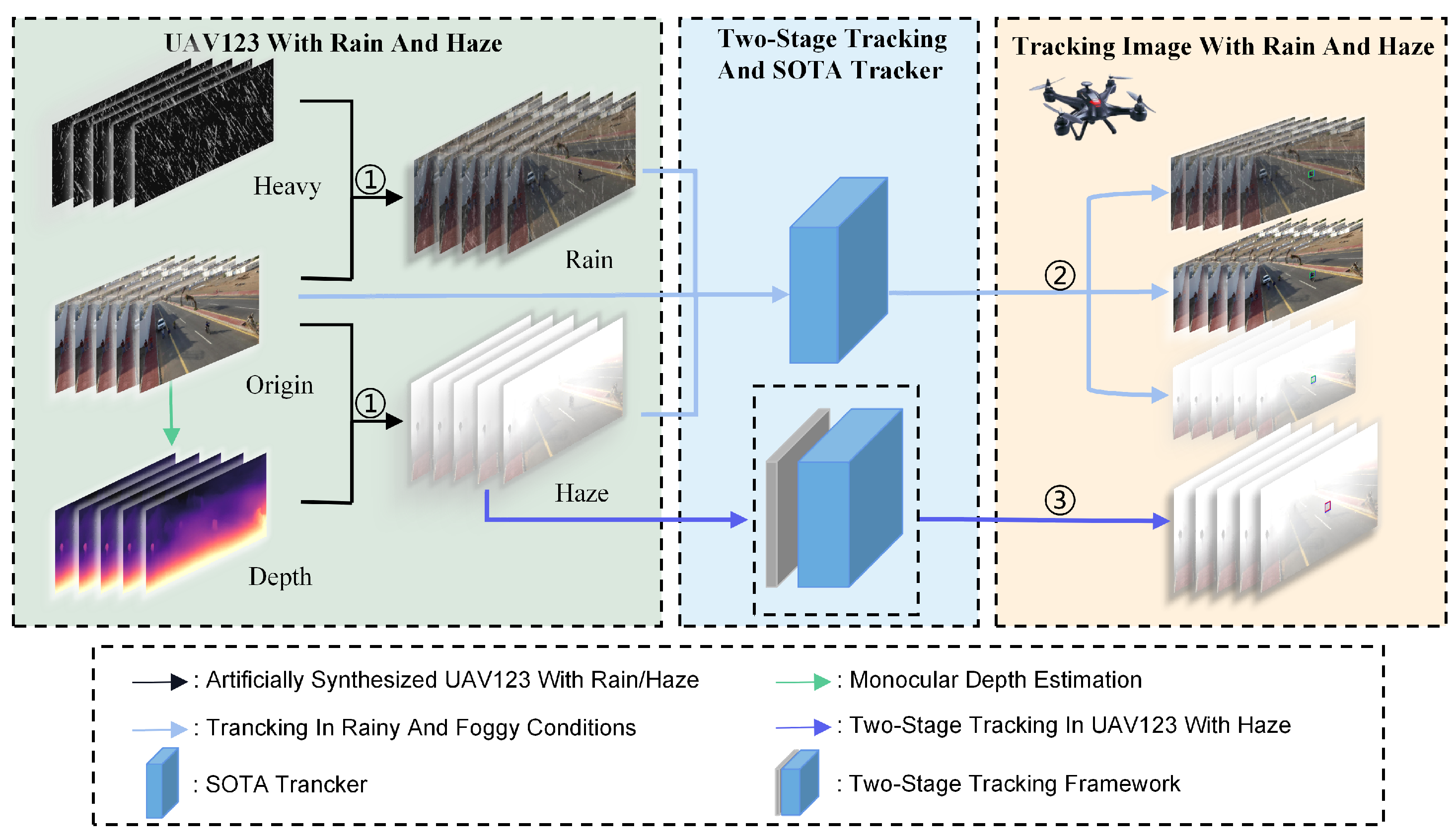
Figure 5.
The pipeline is divided into three sections. (1) denotes artificially synthesized UAV123 [19] with rain and haze. (2) denotes tracking in rainy and foggy conditions with classic methods. (3) denotes applying the two-stage tracking method under identical conditions.
Figure 5.
The pipeline is divided into three sections. (1) denotes artificially synthesized UAV123 [19] with rain and haze. (2) denotes tracking in rainy and foggy conditions with classic methods. (3) denotes applying the two-stage tracking method under identical conditions.

Figure 6.
(a) Overview of the DADNet structure. The image passes through a pre-set convolutional layer and goes through DAB and residual block sequentially, repeated , , and times, respectively. Finally, the MSAB module performs multi-scale fusion on the results of the three modules and outputs intermediate results through a transposed convolution layer. (b) Illustration of the core module named DAB. It adds channel attention and pixel attention after repeated dilated convolutional layers and introduces residual connections.

Figure 7.
The architecture of channel attention and pixel attention. It incorporates batch normalization before the convolutional layer based on the work of our predecessors.
Figure 7.
The architecture of channel attention and pixel attention. It incorporates batch normalization before the convolutional layer based on the work of our predecessors.

Figure 8.
The overall performance of our method and TransT [4] (TransT-N2 in this figure) in adverse weather conditions on the UAV123 [19] dataset. It can be seen that weather conditions have a negative impact on the performance of TransT [4]. As the result of the implementation of our DADNet, an improved performance is obtained, effectively mitigating the negative effects of the adverse weather conditions.

Figure 9.
The overall performance of of our method and OSTrack [6] in adverse weather conditions on the UAV123 [19] dataset. Adverse weather conditions had negative effects on OSTrack [6]. However, the application of DADNet led to a notable enhancement in the tracking, successfully diminishing the impact of harsh weather on the performance.


Table 1.
Five different parameters were used to simulate five different levels of haze interference, with detailed configurations provided in [34] for reference.
Table 1.
Five different parameters were used to simulate five different levels of haze interference, with detailed configurations provided in [34] for reference.
| 170 m | 200 m | 300 m | 350 m | 500 m | |
|---|---|---|---|---|---|
| weather condition | Dense | Thick | Thick | Moderate | Light |
| scattering coef. | 26.1 | 19.6 | 15.5 | 13.7 | 7.8 |
Table 2.
Quantitative comparisons of our proposed network with several other light and classic dehazing networks on the RESIDE [33] indoor dataset. It is apparent that the dehazing accuracy of our network exceeds theirs.
Table 2.
Quantitative comparisons of our proposed network with several other light and classic dehazing networks on the RESIDE [33] indoor dataset. It is apparent that the dehazing accuracy of our network exceeds theirs.
| GRM [62] | CAP [59] | AOD-Net [60] | DeHaze-Net [27] | GFN [61] | GCANet [31] | Ours | |
|---|---|---|---|---|---|---|---|
| PSNR | 18.86 | 19.05 | 19.06 | 21.14 | 22.30 | 30.23 | 31.71 |
| SSIM | 0.8600 | 0.8400 | 0.8504 | 0.8472 | 0.8800 | 0.9800 | 0.9845 |
Table 3.
Tracking performance of SOTA trackers (OSTrack [6], TransT [4]) under light rain and heavy rain conditions. The blue arrows represent performance degradation. It can be observed that rain has minimal impact on tracking performance.
| Tracker | Original Image | Light Rain | Heavy Rain | |||||||||
|---|---|---|---|---|---|---|---|---|---|---|---|---|
| AUC | OP50 | OP75 | Prec. | AUC | OP50 | OP75 | Prec. | AUC | OP50 | OP75 | Prec. | |
| OSTrack | 70.52 | 86.28 | 64.45 | 92.04 | 70.47 | 86.18 | 64.17 | 91.90 | 68.89 | 84.03 | 62.51 | 89.54 |
| TransT | 66.53 | 82.13 | 59.99 | 87.43 | 66.29 | 82.08 | 59.31 | 87.03 | 64.38 | 79.47 | 57.73 | 84.66 |
Table 4.
Performance comparison between the original tracker and our proposed two-stage tracking method in five different levels of foggy environments. The red arrows represent performance improvement. It can be seen that as the concentration of fog increases, the tracking speed (FPS) is not influenced, and the performance gradually declines, but our two-stage tracking method alleviates this problem.
| Weather | OSTrack | DADNet+OSTrack | TransT | DADNet+TransT | ||||||||
|---|---|---|---|---|---|---|---|---|---|---|---|---|
| AUC | Precision | FPS | AUC | Precision | FPS | AUC | Precision | FPS | AUC | Precision | FPS | |
| Origin | 70.52 | 92.04 | 41.4 | 70.41 | 91.82 | 39.3 | 66.53 | 87.43 | 69.1 | 66.46 | 86.89 | 60.7 |
| Light Fog | 67.30 | 88.27 | 41.4 | 67.37 | 91.47 | 39.3 | 63.53 | 84.11 | 69.1 | 63.59 | 84.87 | 60.7 |
| Moderate Fog | 63.36 | 78.16 | 41.4 | 63.50 | 83.97 | 39.3 | 58.96 | 78.26 | 69.1 | 59.47 | 79.64 | 60.7 |
| Thick Fog (15.5) | 60.10 | 74.18 | 41.4 | 61.06 | 80.69 | 39.3 | 56.31 | 74.78 | 69.1 | 58.91 | 79.62 | 60.7 |
| Thick Fog (19.6) | 48.50 | 63.08 | 41.4 | 52.20 | 68.84 | 39.3 | 47.05 | 62.75 | 69.1 | 50.17 | 68.79 | 60.7 |
| Dense Fog | 34.10 | 43.63 | 41.4 | 42.89 | 56.88 | 39.3 | 36.59 | 49.47 | 69.1 | 38.56 | 53.36 | 60.7 |
Table 5.
Ablation experiments on different components of the dehazing backbone on SOTS indoor RESIDE. The table mainly includes attention in dilated convolution, normalization in CA and PA, and SSIM loss.
Table 5.
Ablation experiments on different components of the dehazing backbone on SOTS indoor RESIDE. The table mainly includes attention in dilated convolution, normalization in CA and PA, and SSIM loss.
| Attention in Dilated Conv | ✗ | ✓ | ✓ | ✓ |
| Normalization in CA and PA | ✗ | ✗ | ✓ | ✓ |
| SSIM Loss | ✗ | ✗ | ✗ | ✓ |
| PSNR | 28.63 | 28.92 | 30.31 | 31.71 |
Disclaimer/Publisher’s Note: The statements, opinions and data contained in all publications are solely those of the individual author(s) and contributor(s) and not of MDPI and/or the editor(s). MDPI and/or the editor(s) disclaim responsibility for any injury to people or property resulting from any ideas, methods, instructions or products referred to in the content. |
© 2024 by the authors. Licensee MDPI, Basel, Switzerland. This article is an open access article distributed under the terms and conditions of the Creative Commons Attribution (CC BY) license (https://creativecommons.org/licenses/by/4.0/).
Share and Cite
MDPI and ACS Style
Feng, Y.; Xu, X.; Chen, N.; Song, Q.; Zhang, L. A Two-Stage Method for Aerial Tracking in Adverse Weather Conditions. Mathematics 2024, 12, 1216. https://doi.org/10.3390/math12081216
AMA Style
Feng Y, Xu X, Chen N, Song Q, Zhang L. A Two-Stage Method for Aerial Tracking in Adverse Weather Conditions. Mathematics. 2024; 12(8):1216. https://doi.org/10.3390/math12081216
Chicago/Turabian StyleFeng, Yuan, Xinnan Xu, Nuoyi Chen, Quanjian Song, and Lufang Zhang. 2024. "A Two-Stage Method for Aerial Tracking in Adverse Weather Conditions" Mathematics 12, no. 8: 1216. https://doi.org/10.3390/math12081216
Note that from the first issue of 2016, this journal uses article numbers instead of page numbers. See further details here.