Deep Reinforcement Learning for Network Dismantling: A K-Core Based Approach

Abstract

Network dismantling is one of the most challenging problems in complex systems. This problem encompasses a broad array of practical applications. Previous works mainly focus on the metrics such as the number of nodes in the Giant Connected Component (GCC), average pairwise connectivity, etc. This paper introduces a novel metric, the accumulated 2-core size, for assessing network dismantling. Due to the NP-hard computational complexity of this problem, we propose SmartCore, an end-to-end model for minimizing the accumulated 2-core size by leveraging reinforcement learning and graph neural networks. Extensive experiments across synthetic and real-world datasets demonstrate SmartCore’s superiority over existing methods in terms of both accuracy and speed, suggesting that SmartCore should be a better choice for the network dismantling problem in practice.

1. Introduction

Network dismantling [1] represents a pivotal challenge within the realm of complex network science, drawing sustained attention from a diverse spectrum of researchers over time. This challenge revolves around identifying the minimal subset of nodes whose removal would significantly impair or entirely incapacitate the operational functionality of the network. This problem encompasses a broad array of practical applications. For instance, within power systems, a localized incident such as overload or failure may trigger a cascading series of failures, potentially leading to systemic collapse [2]. However, strategic removal of critical nodes can mitigate this risk and prevent such catastrophic outcomes. In the realms of national security [3] and public health [4], networks such as those associated with terrorist organizations and disease transmission pathways present significant threats.

Network robustness stands as a fundamental metric frequently serving as a yardstick for measuring the degree of network dismantling. A lot of robustness metrics have been proposed in prior studies, spanning from basic graph connectivity metrics (such as node and edge connectivity [5]) to more sophisticated measures of connectivity enhancement (such as super connectivity [6] and conditional connectivity [7]). A comprehensive survey of robustness metrics can be found in [8]. Among these metrics, the concept of K-core [9] emerges as particularly significant and deserving of further investigation. Essentially, in a graph, a K-core embodies a structural attribute wherein a subgraph qualifies as a K-core if each node within that subgraph is connected to a minimum of k other nodes. The K-core configuration plays a pivotal role within networks and is intimately intertwined with graph robustness.

Similarly, the concept of K-core can be applied to the network dismantling problem. Intuitively, if all K-core nodes are removed from a network, it degenerates into a tree structure, which is considerably easier to dismantle [10]. By identifying and removing nodes from the K-core, one can assess the network’s robustness. A network that rapidly disintegrates upon the removal of K-core nodes is considered fragile. The K-core property has sparked the development of several well-known algorithms aimed at addressing the network dismantling challenge. Among these, the CoreHD [11] algorithm stands out as a straightforward yet potent approach. It works by systematically eliminating one of the vertices with the highest degree from the remaining K-core.

Typically, when K = 2, it is referred to as the 2-core. In network dismantling, the 2-core plays a unique role. When the nodes within the 2-core are not empty, it ensures the presence of cyclic structures within the graph; conversely, when the 2-core is empty, the graph degenerates into a tree. Additionally, we have observed changes in the number of nodes in the Giant Connected Component (GCC) and 2-core structure during the dismantling process using four commonly used network dismantling algorithms, as depicted in Figure 1. It is apparent that the GCC and 2-core metrics show a strong correlation throughout the network dismantling process.

Motivated by this observation and drawing an analogy to the definition of the Accumulated Normalized Connectivity (ANC) curve, we propose utilizing the area under the curve of the changing number of nodes in the 2-core structure as a measure of the degree of network dismantling. Minimizing the area under the curve while using the fewest nodes is an NP-hard problem and bears resemblance to the minimum feedback vertex set (or decycling) problem [12], which is a classic NP-complete problem aimed at making the network acyclic at minimal cost.

However, existing research has primarily focused on handcraft-designed algorithms like CoreHD or BPD [13] for addressing the K-core problem. Instead, we formulate this problem as a Markov Decision Process (MDP) and introduce a novel algorithm named SmartCore, which leverages graph neural networks and reinforcement learning to find heuristic strategies that minimize the accumulated 2-core size during the dismantling process. The state corresponds to the network at each moment during dismantling, and the action represents the remaining nodes in the network.

Extensive experiments have been conducted across both synthetic graphs and real-world datasets, with the latter comprising tens of thousands of nodes and edges. The results demonstrate that the proposed SmartCore model generally outperforms existing methods and also exhibits a considerable speed advantage.

In summary, our contributions can be summarized as follows:

• We introduce the evaluation metric of accumulated 2-core size during the network dismantling process. We transform the problem into a learning problem and propose an end-to-end SmartCore model. This model allows training an agent across simple synthetic graphs, which can then be directly applied to real-world datasets.
• We conduct comprehensive experiments to validate our SmartCore model. Our results show that the SmartCore model outperforms state-of-the-art baseline methods in terms of both accuracy and speed.

The remainder of the paper is organized as follows. Section 2 introduces related works of this paper and Section 3 describes the corresponding preliminaries. Section 4 and Section 5 demonstrate our SmartCore model and the experimental setup, respectively. Section 6 provides a summary of our work and outlines future research directions.

2. Related Works

In the realm of complex network analysis, understanding and optimizing network robustness and resilience through network dismantling has become an imperative research area. In the exploration of complex network dismantling, various metrics play a crucial role in understanding the robustness and vulnerability of networks, such as the number of components [14], pairwise connectivity [15], the largest connected component size [16], etc.

Meanwhile, approaches to network dismantling can be categorized into planning-based, metaheuristic, and machine learning methods. Planning-based strategies, as demonstrated [17], utilize mathematical programming to detect critical node structures whose deletion maximally deteriorates the graph’s connectivity, offering a comprehensive framework that extends beyond the removal of individual nodes. Metaheuristic methods can also effectively deal with the network dismantling problem. For instance, Y. Deng et al. [18] proposed an optimal attack strategy named Optimal Attack Strategy (OAS) based on tabu search, which is a global search approach to identify the most destructive node removal combinations. Manuel Lozano et al. used the Artificial Bee Colony (ABC) algorithm [19], which leveraged the knowledge of network dismantling problem in the neighborhood exploration by considering the partial destruction and heuristic reconstruction of selected solutions.

Machine learning approaches, notably through deep reinforcement learning and learning-based algorithms, introduce novel paradigms for identifying key players in network dismantling. These methods, exemplified by FINDER [20,21] and CoreGQN [22], leverage synthetic networks and self-play to train models that significantly outperform existing strategies, offering rapid, scalable solutions to NP-hard problems in network science.

Core structure in complex networks, as an important metric, is also widely researched. Recent advancements include the development of sophisticated attack strategies, such as the Cycle-Tree Guided Attack (CTGA) [23] and the Hierarchical Cycle-Tree Packing Model [24], which utilize spin glass models and efficient message passing algorithms. These methods aim to induce the complete collapse of the k-core by identifying the minimal set of vertices for removal, transforming the dynamics of k-core pruning into a problem of finding optimal static structural patterns.

3. Preliminaries

3.1. K-Core

First, let $G=(V,E)$ be a graph. The k-core of $G$, denoted as $G_k$, is defined as the maximal subgraph $G\prime =(V\prime ,E\prime )$ of $G$, so that every vertex in $V\prime$ has a degree of at least $k$ within $G\prime$.

3.2. Accumulated 2-Core Size

Motivated by the definition of accumulated normalized connectivity (ANC) [25], we can define the learning objective as sequentially removing nodes from the network to minimize the accumulated size of the 2-core after each removal, which we call accumulated 2-core size. Given a graph $G=(V,E)$, let $C_0$ represent the size (number of nodes) of the 2-ore of $G$ before any nodes are removed. For each iteration $i$ where nodes are removed from the graph, let $f_i$ denote the size of the 2-core of the remaining graph. The 2-core size $f_i$ for each iteration $i$ is defined as:

$$f_i=\frac{C_i}{C_0}$$

(1)

The accumulated 2-core size $F$ after $n$ iterations is the sum of $f_i$ across all iterations:

$$F={\displaystyle \sum _{i=1}^n{f}_i}$$

(2)

The objective in our learning task is to minimize the accumulated 2-core size. By doing so, we ensure that as nodes are removed, the remaining graph’s 2-core size is significantly reduced relative to the original 2-core size.

3.3. Graph Neural Network

A Graph Neural Network (GNN) [26] is a type of neural network designed to operate directly on graphs or data that can be represented in graph form. It aims to learn and generalize functions over graph-structured data. The basic idea is to iteratively update node representations by aggregating and propagating information from neighboring nodes.

Mathematically, let $G=(V,E)$ be a graph, where each node $v\in V$ is associated with a feature vector $x_v$. The goal of a GNN is to learn a function, $f$, that maps the input graph $G$ and its node features ${\left\{x_v\right\}}_{v\in V}$ to output predictions or node representations.

The message passing mechanism in GNNs can be described using the following equations:

$$m_v^{(t)}={\mathrm{AGGREGATE}}^{(t)}\left(\left\{h_u^{(t-1)}:u\in \mathcal{N}(v)\right\}\right)$$

(3)

$$h_v^{(t)}={\mathrm{COMBINE}}^{(t)}\left(h_v^{(t-1)},m_v^{(t)}\right)$$

(4)

3.4. Reinforcement Learning

Reinforcement learning (RL) is a branch of machine learning where an agent learns to make sequential decisions by interacting with an environment to maximize cumulative rewards. Q-learning, a fundamental RL algorithm, plays a crucial role in RL by estimating the value of taking a specific action in a given state, enabling the agent to make optimal decisions based on learned Q-values.

Q-learning is an iterative, model-free RL method used to estimate the Q-values of state-action pairs within an MDP, denoted as $\{\mathcal{S},\mathcal{A},\mathcal{T},\mathcal{R},\gamma \}$. Here, $\mathcal{S}$ represents the state space, $\mathcal{A}$ represents the action space, $\mathcal{T}:\mathcal{S}\times \mathcal{A}\times \mathcal{S}\to [0,1]$ is the transition function, $\mathcal{R}:\mathcal{S}\to ℝ$ is the reward function, and $\gamma \in [0,1]$ is the discount factor. The Q-value function, which is an action value function learned by Q-learning methods, maps state-action pairs $(s,a)\in (\mathcal{S},\mathcal{A})$ to the expected discounted sum of rewards when following a policy $\pi :\mathcal{S}\to \mathcal{A},Q^{\pi }(s,a)=\mathbb{E}\left[{\displaystyle \sum _{t=0}^{\infty }{\gamma }^t}{r}_{t+1}\mid s_0=s,a_0=a,\pi \right]$. Compared to traditional Q-learning algorithms, DQN [27] trains a deep neural network $Q_{\theta }$ to approximate the value function. Hence, the policy ${\pi }_{\theta }$ can be determined by: ${\pi }_{\theta }(s)=\arg {\max }_{a^{\prime }}{Q}_{\theta }(s,a^{\prime })$, where $\theta$ is the set of parameters learned by DQN.

4. SmartCore Model

In this section, we present our proposed framework, SmartCore, which is tailored for efficiently minimizing the accumulated 2-core size. Formally, SmartCore treats the process of network dismantling as a Markov Decision Process: the state $s\in S$ represents the remaining 2-core sizes in the current graph, the action $a\in A$ represents removing a node from the remaining 2-core, and the reward $r\in R$ is the relative 2-core size $f_i$ after action $a$ is executed. The termination condition is when the 2-core is empty. We delve into the architecture of SmartCore, elucidate the training process, and discuss its time complexity.

4.1. Architecture of SmartCore

The schematic representation of the SmartCore framework can be visualized in Figure 1. Our proposed SmartCore algorithm adopts a quintessential encoder–decoder architecture.

During the encoding phase, we harnessed the power of GraphSAGE [28] as the feature extraction model for both the entire graph and the selected action nodes. The primary objective here is to transform these intricate graph structures and node details into a comprehensive, dense vector representation. To augment the model’s representational capability, we introduced a virtual node concept, which captures overarching graph characteristics more effectively. Since the parameters of GraphSAGE are independent of specific graph scales, the technique of employing virtual nodes to represent the entire network state can be extended to dynamic graphs, enhancing the flexibility of our model.

During the decoding phase, we employed deep $Q$ learning to the representation of the state and action. The $Q$ function maps state–action pairs to scalar values indicative of potential long-term gains which is parameterized with MLPs coupled with ReLU activation, and makes use of the embeddings to achieve this. This technique ingeniously maps the action node vectors, in conjunction with their respective graph vectors, to a scalar $Q$ value. This $Q$ value serves a pivotal role as it provides a quantifiable metric, guiding the subsequent action selection process. The agent, equipped with this strategy, then embarks on an iterative journey where it greedily selects the node boasting the highest $Q$ value at each step. This meticulous node removal continues iteratively until the network is devoid of any cycles, ensuring an acyclic structure. Through this intricate blend of GraphSAGE for feature extraction and the deep Q-learning for decision making, SmartCore provides a robust solution to tackle complex network challenges (Figure 2).

4.2. Training Algorithms

The computation of the Q-score is contingent on a set of six parameters, denoted as $\Theta ={\left\{{\theta }_i\right\}}_{i=1}^6$. We employed Double Q-Learning [29] to train the model. Specifically, Double Q-Learning refines the parameters by undertaking gradient descents on samples (or mini batches) of experience $(s,a,r,s^{\prime })$, aiming to curtail the loss, which is defined as follows:

$$\mathrm{Loss}={\mathbb{E}}_{(s,a,r,s^{\prime })~U(D)}\left[{\left(r+\gamma Q\left(s^{\prime },{\mathrm{argmax}}_{a^{\prime }}Q(s^{\prime },a^{\prime })\right)-Q(s,a)\right)}^2\right]$$

(5)

Here, the samples $(s,a,r,s^{\prime })$ were selected uniformly at random from the pool of stored samples $U(D)$, where $D=\{d_1,d_2,\dots ,d_t\},d_t=(s_t,a_t,r_t,s_{t+1})$, and $\widehat{Q}$ represents the target network, with parameters that become updated from the $Q$ network parameters every $C$ steps, while remaining constant between individual updates.

During the training phase, the Barabási–Albert (BA) model generates synthetic graphs for both training and validation purposes. An episode represents the entire node removal process on a graph until the terminal state is reached. The terminal state, in this context, is when the 2-core node count becomes zero. A trajectory created within an episode refers to a state–action sequence $(s_0,a_0,r_0,s_1,r_1,s_2,\dots ,s_{\mathrm{terminal}})$.

Training adopts the $ϵ$-greedy policy, where $ϵ$ linearly tapers from 1.0 to 0.01 over 10,000 episodes to strike a balance between exploration and exploitation. In the inference phase, the node with the highest Q-score is systematically removed until the terminal state is reached.

The model underwent training for a total of 50,000 episodes. A replay memory, with a capacity of 20,000, retained the most recent transitions. Every 300 episodes, we evaluated the agent across 100 synthetic graphs of the same size as the training graphs, averaging the performances. After each episode, random mini batches of transitions were drawn from the replay memory buffer to perform stochastic gradient descent updates that minimize the loss function. The entire training procedure is elaborated in detail in Algorithm 1.

Algorithm 1: Training Procedure of SmartCore

1: Initialize experience replay memory $D$ with size $M$ 2: Initialize state–action pair value function $Q$ with random weights $\omega$ 3: Initialize target $Q$ function with weights $\widehat{\Theta }=\Theta$ 4: For episode = 1 to $N$ Do 5:  Generate a graph $G$ from the BA model 6:  Obtain the 2-core $G\prime$ from $G$ 7:  Initialize the state to an empty sequence $s_1=()$ 8:  For $t$ = 1 to $T$ Do 9:   With probability $ϵ$, select a random action $a_t$ on $G\prime$ 10:   Otherwise select $a_t={\mathrm{argmax}}_{a}Q(s_t,a;\Theta )$ 11:   Execute action $a_t$ (remove node $a_t$ from $G\prime$) and observe reward $r_t$ 12:   Add $a_t$ to partial solution $s_{t+1}=s_t\cup a_t$ 13:   If $t>n$ Then 14:    Store transition $(s_t,a_t,r_t,s_{t+1})$ in $D$ 15:    Sample random mini–batch of transitions $(s_j,a_j,r_j,s_{j+1})$ from $D$ 16:    $\mathrm{Set} y_j=\left\{\begin{array}{c}{r}_j \mathrm{If} \mathrm{eposide} \mathrm{terminates} \mathrm{at} \mathrm{step} j+1\\ r_j+\gamma Q\left(s^{\prime },{\mathrm{argmax}}_{a^{\prime }}Q(s^{\prime },a^{\prime };\Theta );\widehat{\Theta }\right) \mathrm{Otherwise} \end{array}\right.$ 17:    Perform a stochastic gradient descent over (3) with respect to the parameters $\Theta$ 18:    Every $C$ steps reset $\widehat{\Theta }=\Theta$ 19:   End If 20:   Update the 2-core size from $G$ 21:  End For 22: End For

4.3. Computational Complexity Analysis

The overall time complexity of the SmartCore model is denoted as $O(T|E|t)$. Here, $T$ denotes the depth of the GraphSAGE layers, $\left|E\right|$ represents the number of edges in the graph, and $t$ denotes the total number of nodes removed while the 2-core is empty. By using sparse matrix representations for the graph, our SmartCore model can easily scale to large-scale graphs in real-world applications.

5. Experiments

5.1. Baselines

To validate the efficacy of the proposed SmartCore algorithm, we employed the currently prevalent algorithms HDA [30], HBA [31], HCA [32], and HPRA [33] as benchmark methods across simulated graphs. Using the BA network (with m = 4), we generated 100 simulated graphs for node ranges of 30–50, 50–100, 100–200, 200–300, 300–400, and 400–500 to evaluate the performance of the algorithm across simulated networks. Specifically, HDA refers to an approach where the node with the highest degree is removed from the network in each iteration. The network was then updated, and the node degrees were recalculated, continuing this process until no cycles remained in the network. Similarly, HBA removed the node with the highest betweenness centrality in each iteration, HPRA removed the node with the highest PageRank, and HCA removed the node with the highest closeness centrality. After each node removal, the respective metric was recalculated based on the updated network, and the process continued until the network was acyclic.

For testing across real networks, we selected he HDA [30], CI [34], MinSum [35], CoreHD [11], BPD [13], and GND [36] as our benchmark methods. CI represents an index based on collective influence. MinSum and BPD are decycling algorithms based on belief propagation, while GND is an algorithm rooted in spectral partitioning. Specifically, CoreHD operates by removing the node with the highest 2-core degree during each iteration. After each removal, the 2-core was updated, node degrees within the 2-core were recalculated, and the process was repeated until the 2-core was empty.

5.2. Datasets

Four real-world datasets were selected from SNAP Datasets [37] to evaluate the performance of our SmartCore model, as shown in

Table 1. Detailed description of four real-world datasets.

Data/Index	Node Number	Edge Number	Diameter
HI–II–14	4165	13,087	11
Digg	29,652	84,781	12
Enron	33,696	180,811	11
Epinion	75,879	508,837	14

:

HI–II–14: This dataset encompasses the Human Interactome data in Space II, compiled in 2014.

Digg: This network mirrors interactions on the social news platform, Digg.

Enron: This dataset captures the email communication patterns within the Enron corporation, spanning approximately half a million emails.

Epinion: Originating from the online social network, Epinions, this trust network outlines user interactions.

5.3. Training Details

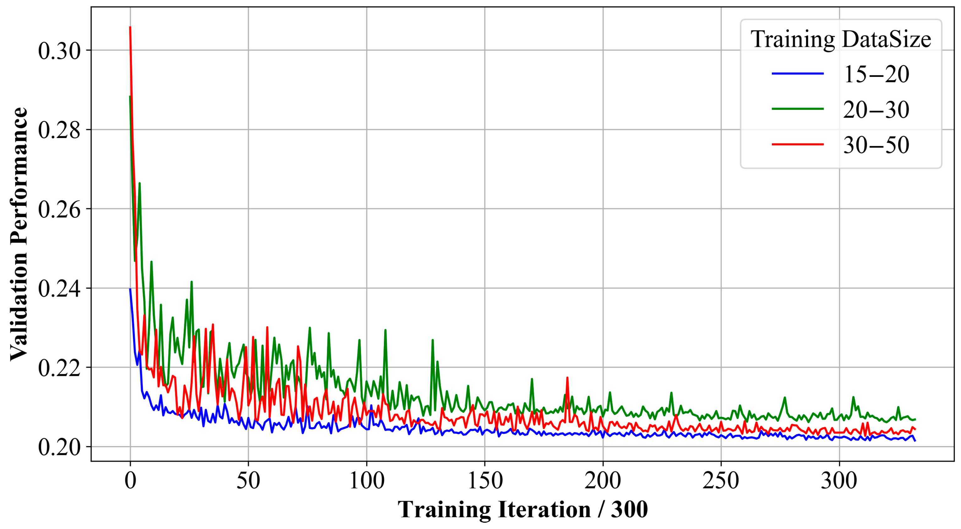
All our experimental tasks were executed on a platform equipped from Huawei Cloud with a 32 GB Nvidia GeForce Tesla A100 GPU. For training and validation, we utilized Barabási–Albert (BA) graphs generated by the networkx package (v2.8.8) and set the parameter m as 4, which means the number of edges linking a new node to existing ones; the size of the nodes was between 30 and 50. Given that real-world graphs usually adhere to power–law distribution, they can be effectively simulated through the BA graphs. The performance of SmartCore across real graphs also validates the rationality of the training data generation strategy we employed. In total, 10,000 synthetic graphs were created for training purposes, while another 100 were earmarked for validation. To test the performance of SmartCore across different scales of synthetic graphs, we generated 100 graphs for each scale of 30–50, 50–100, 100–200, 200–300, 300–400, and 400–500, following the setting described above. The hyper parameters of SmartCore are shown in

Table 2. Hyper parameter Settings for SmartCore.

Name	Value	Description
Learning rate	1 × 10−4	The learning rate used by Adam optimizer
Embedding dimension	64	Dimensions of node embedding vector
Layer iterations	5	Number of GraphSAGE layers
Q-learning steps	3	Number of Q-learning steps
Batch size	64	Number of mini-batch training samples

. We developed our model using Pytorch Version 1.9 and adopted the Adam optimization method for training. An early stopping mechanism, based on the validation of the set performance, ensured efficient training. As can be observed in Figure 3, the model exhibits impressive convergence for the given problem.

5.4. Results

Figure 4 presents the testing results of SmartCore compared with benchmark algorithms HDA, HBA, HCA, and HPRA across 100 synthetic graphs of varying sizes. From the figure, it is evident that SmartCore outperforms the other methods. Additionally,

Table 3. The running time of different methods across six synthetic datasets.

Method/Data Size	30–50	50–100	100–200	200–300	300–400	400–500
HDA	59.80 ± 3.36	59.36 ± 3.00	57.62 ± 1.99	56.97 ± 1.49	56.57 ± 1.36	56.50 ± 1.10
HBA	79.67 ± 9.69	84.37 ± 7.71	88.97 ± 5.55	91.18 ± 4.30	93.08 ± 3.74	92.97 ± 3.45
HCA	62.12 ± 4.26	61.34 ± 2.93	59.65 ± 2.01	58.99 ± 1.66	58.76 ± 1.42	58.53 ± 1.36
HPRA	60.12 ± 3.24	59.35 ± 3.06	58.04 ± 1.96	57.22 ± 1.53	56.85 ± 1.33	56.89 ± 1.19
SmartCore	65.21 ± 3.88	62.26 ± 3.06	59.45 ± 1.82	57.81 ± 1.46	57.30 ± 1.30	57.31 ± 1.16

displays the runtime of SmartCore and the other benchmark algorithms on this dataset, highlighting that SmartCore boasts a faster execution speed.

Table 4. The accumulated 2-core sizes of different methods across six real-world datasets.

Method/Dataset	HI–II–14	Digg	Enron	Epinions
HDA	0.0482	0.3017	0.3250	0.0507
CI	0.0581	0.2547	0.3263	0.0840
MinSum	0.0615	0.2207	0.3344	0.1028
CoreHD	0.0454	0.2241	0.3278	0.0464
BPD	0.0541	0.2207	0.3259	0.0641
GND	0.0730	0.2392	0.3361	0.0905
SmartCore	0.0459	0.0660	0.0924	0.0504

and

Table 5. The running time of different methods across six real-world datasets.

Method/Dataset	HI–II–14	Digg	Enron	Epinions
HDA	0.78	117.23	139.30	311.70
CI	1.96	113.96	135.42	835.78
MinSum	2.03	113.32	134.82	876.25
CoreHD	2.03	112.73	136.72	893.14
BPD	2.02	114.24	136.08	895.85
GND	2.02	115.22	136.67	864.12
SmartCore	1.15	60.34	73.30	335.88

provide insights into the performance of various algorithms, including the proposed SmartCore, when applied to six real-world datasets.

From Table 4, which displays the accumulated 2-core size for each method across different datasets, we observe that SmartCore consistently achieves lower values, implying a more efficient dismantling of the network’s core structure. In particular, for datasets like Digg and Enron, SmartCore’s performance is significantly superior, reducing the 2-core size by a considerable margin when compared to other methods.

Table 5, on the other hand, focuses on the running time of these algorithms. Here, we see that SmartCore not only offers competitive performance in terms of effectiveness but also in terms of efficiency. For instance, in the Digg dataset, SmartCore completes its task in just 60.34 units of time, which is almost half the time taken by many other algorithms. This trend is similarly observed in the Enron dataset, showcasing the algorithm’s capability to deliver results faster.

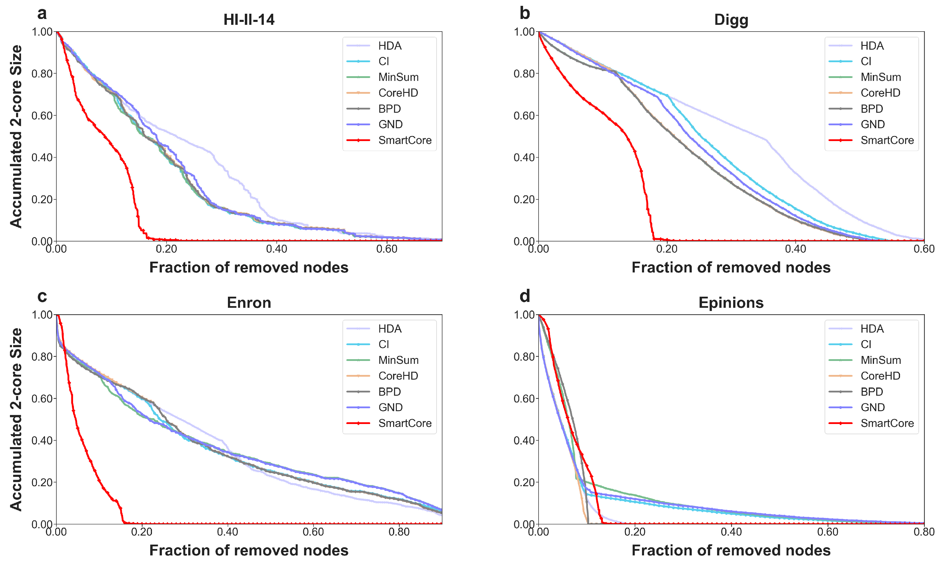
Figure 5 presents a comparison of the accumulated 2-core size curves across real-world networks. The figure’s horizontal axis quantifies the fraction of nodes that have been removed, while the vertical axis represents the remaining 2-core size. From the curves depicted in the figure, it is evident that the SmartCore algorithm consistently maintains a smaller area under its curve across all four real-world datasets. In essence, the results in Figure 5 underscore the outstanding performance of the SmartCore algorithm in comparison to other methods.

6. Conclusions

In this study, we introduced SmartCore, an innovative algorithm that combines graph representation learning with reinforcement learning to tackle the network dismantling problem by minimizing the accumulated 2-core size. Through a sophisticated encoder–decoder architecture, SmartCore efficiently maps graph structures to dense vectors using GraphSAGE, and subsequently employs Double DQN to guide the node selection strategy.

Our extensive experiments, both on synthetic and real-world datasets, have demonstrated the superiority of SmartCore in comparison to prevailing state-of-the-art methods. Not only does SmartCore consistently achieve a smaller accumulated 2-core size, but it also showcases impressive computational efficiency, as evidenced by its faster running times on several datasets. The use of a virtual node to capture graph-level features notably enhanced the algorithm’s representation capabilities. Meanwhile, the transition from a traditional Q-learning approach to Double DQN in the decoder phase further optimized the decision-making process, leading to more effective node removals.

Looking ahead, the success of SmartCore sets a promising precedent for leveraging the power of graph neural networks and advanced reinforcement learning techniques in network dismantling and other related optimization tasks. In future research, we plan to explore how SmartCore’s approach can be adapted to address diverse graph-based challenges. This includes investigating its application in dynamic network scenarios and exploring additional graph-level features to enhance performance.

References

- Albert, R.; Barabási, A.L. Statistical mechanics of complex networks. Rev. Mod. Phys. 2002, 74, 47. [Google Scholar] [CrossRef]
- Yang, Y.; Nishikawa, T.; Motter, A.E. Small vulnerable sets determine large network cascades in power grids. Science 2017, 358, eaan3184. [Google Scholar] [CrossRef]
- Fan, C.; Xiao, K.; Xiu, B.; Lv, G. A fuzzy clustering algorithm to detect criminals without prior information. In Proceedings of the 2014 IEEE/ACM International Conference on Advances in Social Networks Analysis and Mining (ASONAM 2014), IEEE, Beijing, China, 17–20 August 2014. [Google Scholar]
- Pastor-Satorras, R.; Vespignani, A. Epidemic spreading in scale-free networks. Phys. Rev. Lett. 2001, 86, 3200. [Google Scholar] [CrossRef] [PubMed]
- Frank, H.; Frisch, I. Analysis and design of survivable networks. IEEE Trans. Commun. Technol. 1970, 18, 501–519. [Google Scholar] [CrossRef]
- Bauer, D.; Boesch, F.; Suffel, C.; Tindell, R. Connectivity extremal problems and the design of reliable probabilistic networks. Theory Appl. Graphs 1981, 89–98. [Google Scholar]
- Harary, F. Conditional connectivity. Networks 1983, 13, 347–357. [Google Scholar] [CrossRef]
- Wu, J.; Barahona, M.; Tan, Y.J.; Deng, H.Z. Spectral measure of structural robustness in complex networks. IEEE Trans. Syst. Man Cybern. Part A Syst. Hum. 2011, 41, 1244–1252. [Google Scholar] [CrossRef]
- Dorogovtsev, S.N.; Goltsev, A.V.; Mendes, J.F. K-core organization of complex networks. Phys. Rev. Lett. 2006, 96, 040601. [Google Scholar] [CrossRef]
- Cohen, R.; Havlin, S. Complex Networks: Structure, Robustness and Function; Cambridge University Press: Cambridge, UK, 2010. [Google Scholar]
- Zdeborová, L.; Zhang, P.; Zhou, H.J. Fast and simple decycling and dismantling of networks. Sci. Rep. 2016, 6, 37954. [Google Scholar] [CrossRef]
- Fomin, F.V.; Gaspers, S.; Pyatkin, A.V.; Razgon, I. On the Minimum Feedback Vertex Set Problem: Exact and Enumeration Algorithms. Algorithmica 2008, 52, 293–307. [Google Scholar] [CrossRef]
- Mugisha, S.; Zhou, H. Identifying optimal targets of network attack by belief propagation. Phys. Rev. E 2016, 94, 012305. [Google Scholar] [CrossRef]
- Addis, B.; Di Summa, M.; Grosso, A. Identifying critical nodes in undirected graphs: Complexity results and polynomial algorithms for the case of bounded treewidth. Discret. Appl. Math. 2013, 161, 2349–2360. [Google Scholar] [CrossRef]
- Arulselvan, A.; Commander, C.W.; Elefteriadou, L.; Pardalos, P.M. Detecting critical nodes in sparse graphs. Comput. Oper. Res. 2009, 36, 2193–2200. [Google Scholar] [CrossRef]
- Li, H.; Shang, Q.; Deng, Y. A generalized gravity model for influential spreaders identification in complex networks. Chaos Solitons Fractals 2021, 143, 110456. [Google Scholar] [CrossRef]
- Walteros, J.L.; Veremyev, A.; Pardalos, P.M.; Pasiliao, E.L. Detecting critical node structures on graphs: A mathematical programming approach. Networks 2019, 73, 48–88. [Google Scholar] [CrossRef]
- Deng, Y.; Wu, J.; Tan, Y.J. Optimal attack strategy of complex networks based on tabu search. Phys. A Stat. Mech. Its Appl. 2016, 442, 74–81. [Google Scholar] [CrossRef]
- Lozano, M.; Garcia-Martinez, C.; Rodriguez, F.J.; Trujillo, H.M. Optimizing network attacks by artificial bee colony. Inf. Sci. 2017, 377, 30–50. [Google Scholar] [CrossRef]
- Fan, C.; Zeng, L.; Sun, Y.; Liu, Y.Y. Finding key players in complex networks through deep reinforcement learning. Nat. Mach. Intell. 2020, 2, 317–324. [Google Scholar] [CrossRef]
- Zeng, L.; Fan, C.; Chen, C. Leveraging Minimum Nodes for Optimum Key Player Identification in Complex Networks: A Deep Reinforcement Learning Strategy with Structured Reward Shaping. Mathematics 2023, 11, 3690. [Google Scholar] [CrossRef]
- Fan, C.; Zeng, L.; Feng, Y.; Cheng, G.; Huang, J.; Liu, Z. A novel learning-based approach for efficient dismantling of networks. Int. J. Mach. Learn. Cybern. 2020, 11, 2101–2111. [Google Scholar] [CrossRef]
- Zhou, H.-J. Cycle-tree guided attack of random K-core: Spin glass model and efficient message-passing algorithm. Sci. China Phys. Mech. Astron. 2022, 65, 230511. [Google Scholar] [CrossRef]
- Zhou, J.; Zhou, H.J. Hierarchical Cycle-Tree Packing Model for Optimal K-Core Attack. J. Stat. Phys. 2023, 190, 200. [Google Scholar] [CrossRef]
- Schneider, C.M.; Moreira, A.A.; Andrade, J.S., Jr.; Havlin, S.; Herrmann, H.J. Mitigation of malicious attacks on networks. Proc. Natl. Acad. Sci. USA 2011, 108, 3838–3841. [Google Scholar] [CrossRef] [PubMed]
- Zhou, J.; Cui, G.; Hu, S.; Zhang, Z.; Yang, C.; Liu, Z.; Wang, L.; Li, C.; Sun, M. Graph neural networks: A review of methods and applications. AI Open 2020, 1, 57–81. [Google Scholar] [CrossRef]
- Mnih, V.; Kavukcuoglu, K.; Silver, D.; Rusu, A.A.; Veness, J.; Bellemare, M.G.; Graves, A.; Riedmiller, M.; Fidjeland, A.K.; Ostrovski, G.; et al. Human-level control through deep reinforcement learning. Nature 2015, 518, 529–533. [Google Scholar] [CrossRef] [PubMed]
- Hamilton, W.; Ying, Z.; Leskovec, J. Inductive Representation Learning on Large Graphs. In Proceedings of the 31st Annual Conference on Neural Information Processing Systems (NIPS 2017), Long Beach, CA, USA, 4–9 December 2017. [Google Scholar]
- Hasselt, H. Double Q-learning. In Advances in Neural Information Processing Systems; Neural Information Processing Systems Foundation, Inc. (NeurIPS): La Jolla, CA, USA, 2010; Volume 23. [Google Scholar]
- Hooshmand, F.; Mirarabrazi, F.; MirHassani, S.A. Efficient Benders Decomposition for Distance–Based Critical Node Detection Problem. Omega 2020, 93, 102037. [Google Scholar] [CrossRef]
- Carmi, S.; Havlin, S.; Kirkpatrick, S.; Shavitt, Y.; Shir, E. A Model of Internet Topology Using K –Shell Decomposition. Proc. Natl. Acad. Sci. USA 2007, 104, 11150–11154. [Google Scholar] [CrossRef] [PubMed]
- Bavelas, A. Communication Patterns in Task-Oriented Groups. J. Acoust. Soc. Am. 1950, 22, 725–730. [Google Scholar] [CrossRef]
- Wandelt, S.; Sun, X.; Feng, D.; Zanin, M.; Havlin, S. A Comparative Analysis of Approaches to Network–Dismantling. Sci. Rep. 2018, 8, 13513. [Google Scholar] [CrossRef]
- Morone, F.; Makse, H.A. Influence maximization in complex networks through optimal percolation. Nature 2015, 524, 65–68. [Google Scholar] [CrossRef]
- Braunstein, A.; Dall’Asta, L.; Semerjian, G.; Zdeborová, L. Network Dismantling. Proc. Natl. Acad. Sci. USA 2016, 113, 12368–12373. [Google Scholar] [CrossRef] [PubMed]
- Ren, X.; Gleinig, N.; Helbing, D.; Antulov–Fantulin, N. Generalized network dismantling. Proc. Natl. Acad. Sci. USA 2018, 116, 6554–6559. [Google Scholar] [CrossRef] [PubMed]
- Leskovec, J.; Krevl, A. SNAP Datasets: Stanford Large Network Dataset Collection; SNAP: Santa Monica, CA, USA, 2014. [Google Scholar]
Figure 1.
Case study of the relationship between GCC size and 2-core size during network dismantling. We generate 100 graphs using the Barabási–Albert model and calculate the average GCC size and 2-core size.
Figure 2.
SmartCore Framework Overview. The SmartCore framework encompasses a typical encoder–decoder structure. Within this setup, the encoder leverages GraphSAGE to transform the raw input of the graph into a compact embedding. Subsequently, the Double DQN decoder processes the graph embedding in tandem with the action node’s embedding to produce a value. This value serves as a guiding metric for the node selection strategy in subsequent steps.
Figure 3.
SmartCore’s performance Cureve. As gauged by validation results, SmartCore demonstrates a rapid convergence during its training process. We trained our agent on synthetic BA graphs across various scales, specifically with node sizes ranging from 15 to 20, 20 to 30, and 30 to 50, and validated on corresponding scales. In each iteration, 64 synthetic graphs were sampled for training. After every 300 iterations, we evaluated the model across 100 randomly chosen graphs. The metric of interest was the accumulated 2-core size. Across all training scales, SmartCore consistently demonstrated swift convergence across the validation datasets.
Figure 4.
Accumulated 2-core sizes of different methods across six synthetic graphs.
Figure 5.
Comparative results of the accumulated 2-core size curves across real-world networks (a–d). The horizontal axis is the fraction of the removed nodes, and the vertical axis is the remaining 2-core size.