Estimating the Individual Treatment Effect with Different Treatment Group Sizes

Abstract

Machine learning for causal inference, particularly at the individual level, has attracted intense interest in many domains. Existing techniques focus on controlling differences in distribution between treatment groups in a data-driven manner, eliminating the effects of confounding factors. However, few of the current methods adequately discuss the difference in treatment group sizes. Two approaches, a direct and an indirect one, deal with potential missing data for estimating individual treatment with binary treatments and different treatment group sizes. We embed the two methods into certain frameworks based on the domain adaption and representation. We validate the performance of our method by two benchmarks in the causal inference community: simulated data and real-world data. Experiment results verify that our methods perform well.

1. Introduction

What outcome an intervention produces, i.e., causal inference, has been a critical research topic across many domains. In traditional statistical methods, most causal inference studies are grounded in the average causal effect of the aggregate or subgroup to obtain the causal characteristics of the population [1,2,3]. For example, researchers are interested in the average preventive effect of flu vaccination on the population, the carcinogenic effect of smoking on the smoking population, and the effect of running on body fat in men and women, respectively. However, with the development of modern statistics and the advent of the era of big data, the increasing requirements for personalized decision making, such as achieving individual precision treatment and precise placement strategies for internet advertising, have emerged. More researchers have realized that the method of causal inference from the overall population is no longer applicable and have become concerned with individual-level treatment effects (or heterogeneous effects) [4,5].

Various frameworks for causal inference have been developed, the most representative of which are the potential outcome framework [6,7] and the structural causal model [8]. In this paper, we focus on the potential outcome framework which is proposed when the intervention and outcome variables are known. For binary treatments $t\in \{0,1\}$, we assume that the outcomes of individual i with treatment t are unique and unaffected by other individuals. Such outcomes are referred to as the potential outcome denoted by $Y_t$. We characterize each individual (also known as a unit) by a vector of context $x_i\in \mathcal{X}$, denote $m_1\left(x\right)=E\left[Y_1\right|X=x]$, $m_0\left(x\right)=E\left[Y_0\right|X=x]$, and focus on the function $\tau \left(x\right)=m_1\left(x\right)-m_0\left(x\right)$. $\tau \left(x\right)$ is the Individual Treatment Effect (ITE), reflecting the expected treatment effect of $t=1$ relative to $t=0$ on a unit with context x. However, for each individual, we never observe both $Y_1$ and $Y_0$ in the real world, which is a major challenge for causal inference. The statisticians overcame this problem by designing randomized studies, making such treatment effects identifiable [9].

However, researchers in many fields often make causal inferences based on observational studies due to the low availability of randomized controlled trials (RCT). Observational data are based on empirical observations and cannot use controlled experiments or randomly assigned treatments [10]. In observational studies, both potential outcomes and treatments are influenced by certain factors, which are known as confounding factors. Ignoring these factors can lead to biases and even paradoxes, which is another major challenge for estimating treatment effects [11,12]. For example, both children’s shoe size and vocabulary are affected by age. If the age variable is ignored, it may be absurd to conclude that the size of shoes can affect vocabulary. The important strong ignorability assumption was introduced to make the conditional causal effect identifiable in observational studies.

Indeed, when estimating treatment effects from observational data, we face two problems, i.e., missing counterfactual outcomes and confounding bias. Many methods for estimating ITE based on deep representation learning have been proposed to address the above two problems. An inspiring general framework is the Counterfactual Regression (CFR) method, where the first generalization-error upper bound for estimating ITE is given [13]. The upper bound, consisting of the error of learning $Y_1$ and $Y_0$ and a measure of the distance between two distributions $p\left(x\right|t=1)$ and $p\left(x\right|t=0)$, has similarities with generalization bounds in domain adaptation [14,15]. Based on such an ITE error upper bound, many recent methods have focused on learning representations regularized to balance confounding factors by enforcing domain invariance with distributional distances. For example, Feature Selection Representation Matching(FSRM) adopts deep feature selection and incorporates a regularizer based on the Integral Probability Metric (IPM) measure to learn balanced representations [16]. In addition, a subsequent research approach argues that domain-invariance regularizer based on IPM is too strict and introduces a novel regularization criterion by interpreting the loss of predictive power of domain-invariance representation as a loss of information in the input variables [17].

The number of actual exposures observed in the data is often very small in the real world due to exogenous variables. For example, the number of cancer patients in hospitals who choose to undergo expensive treatment is usually a small percentage, as it usually depends on the patient’s income level. The difficulties that arise when the probability of treatment is near zero are commonly referred to as violations of the overlap assumption [18]. In the case of binary treatments, although the above violations rarely occur, the sample sizes of the treated and control groups are often imbalanced, i.e., the overlap is poor. In this case, we argue that estimators of treatment effects are not able to generalize or transport causal findings beyond an experimental setting.

In this paper, we formally define the DTGS task as estimating individual treatment effects with different treatment group sizes. Our work is distinct from machine learning based on imbalanced datasets [19,20,21]. We focus predominantly on estimating ITE more efficiently in the DTGS task by calibrating the sample difference between treated and control groups. We propose two simple yet effective techniques for addressing DTGS: Minority in Treatment Over-sampling (MTOVA) and Factual Outcome Distribution Smoothing (FODS). Both approaches can be easily integrated into certain existing representation learning approaches for ITE estimation. A key idea underlying them is to compensate directly or indirectly for potential missing parts of the observed sample based on the above first ITE generalization-error upper bound. MTOVA is proposed from a data perspective, while FODS is proposed from an algorithmic perspective.

To verify the effectiveness of MTOVA and FODS, we conduct experiments on two well-known public datasets of causal inference. The results show that certain existing representation learning approaches for estimating ITE in combination with the two techniques outperform themselves in the DTGS task. The main contributions of this research are:

• We define the DTGS task as learning ITE from observational data with different treatment group sizes;
• The two approaches developed in this paper, MTOVA and FODS, are easily embedded in the existing framework for estimating ITE and can contribute to a more efficient estimation of ITE in DTGS;
• We conduct experiments on a simulated dataset and a real-world dataset to validate the effectiveness of our two methods.

2. Methods

2.1. Problem Setting

The space of covariates vector x is a bounded set $\mathcal{X}\subset {\mathbb{R}}^d$ with distribution $p\left(x\right)$ and the space of continuous outcome is $\mathcal{Y}\subset \mathbb{R}$. Suppose that the observational data contain n units and each unit receives binary treatments $t\in \{0,1\}$. For each unit, $t_i=1$ means the treated group and $t_i=0$ means the control group. We assume that the potential outcome of unit i with treatment t which is denoted by $Y_t$ is unique and unaffected by other individuals (Stable Unit Treatment Value Assumption, SUTVA). In the observational study, we face two major challenges in estimating treatment effects, as follows:

• We never observe both $Y_1$ and $Y_0$ for each unit in the real world, i.e., missing the counterfactual outcomes;
• Confounding factors produce confounding bias, leading to invalid treatment effect predictions.

Let $\mathcal{D}={\left\{(t,Y_i,x_i)\right\}}_{i=1}^N$ be an observed dataset, where the treatment group has a total of m samples and the control group has a total of n samples, with $m+n=N$. We define DTGS below.

Definition 1 (DTGS).

If m:n or n:m exceeds 4:1, estimating the ITE with this dataset $\mathcal{D}$ is called the DTGS task.

2.2. Definitions, Assumptions, and Lemmas

Technical background in this paper including the definitions, assumptions, and lemmas are introduced as follows.

Assumption 1 (Consistency). 

The potential outcome of treatment t is equal to the observed outcome if the actual treatment received is t.

Assumption 2

(Strong ignorability [22]). Given covariates x, treatment assignment T is independent to the potential outcomes, i.e., $(Y_0,Y_1)\perp \perp t\mid x$, and $0<p(t=1\mid x)<1$.

Definition 2.

The average treatment effect (ATE) is:

$$ATE=E(Y_1-Y_0)=E\left[E(Y_1-Y_0|x)\right].$$

(1)

Definition 3.

The treatment effect for unit x (ITE) is:

$$\tau \left(x\right):=E[Y_1-Y_0|x].$$

(2)

Definition 4.

The treated and control group distributions are:

$$\begin{array}{cc}\hfill & p^{t=1}\left(x\right):=p\left(x\right|t=1),\hfill \\ \hfill & p^{t=0}\left(x\right):=p\left(x\right|t=0).\hfill \end{array}$$

(3)

For observational data, the two distributions in Equation (3) are often significantly distinct due to confounding factors.

Definition 5.

Let $\mathsf{\Phi }:\mathcal{X}\to \mathcal{R}$ be a one-to-one representation function and h: $\mathcal{R}\times \{0,1\}\to \mathcal{Y}$ be a hypothesis over the representation space $\mathcal{R}$. Let L: $\mathcal{Y}\times \mathcal{Y}\to {\mathbb{R}}_{+}$ be a loss function. The expected loss for the unit and treatment pair (x,t) is:

$$l_{h,\mathsf{\Phi }}(x,t)={\int }_{\mathcal{Y}}L(Y_t,h(\mathsf{\Phi }\left(x\right),t))p\left(Y_t\right|x)dy.$$

(4)

Definition 6.

The expected treated and control losses are:

$$\begin{array}{c}\hfill {ϵ}_F^{t=1}(h,\mathsf{\Phi })={\int }_{\mathcal{X}}{l}_{h,\mathsf{\Phi }}(x,1)p^{t=1}\left(x\right)dx,\\ \hfill {ϵ}_F^{t=0}(h,\mathsf{\Phi })={\int }_{\mathcal{X}}{l}_{h,\mathsf{\Phi }}(x,0)p^{t=0}\left(x\right)dx.\end{array}$$

(5)

Definition 7.

Let f: $\mathcal{X}\times \{0,1\}\to \mathcal{Y}$ be a hypothesis. The treatment effect estimate of the hypothesis f for unit x is:

$$\begin{array}{cc}\hfill {\widehat{\tau }}_f\left(x\right)& =f(x,1)-f(x,0).\hfill \end{array}$$

(6)

Definition 8.

The expected Precision in Estimation of Heterogeneous Effect (PEHE, [23]) of f is:

$$\begin{array}{c}\hfill {ϵ}_{\mathrm{PEHE}}\left(f\right)={\int }_{\mathcal{X}}{({\tau }_f\left(x\right)-{\widehat{\tau }}_f\left(x\right))}^{2}p\left(x\right)dx.\end{array}$$

(7)

Definition 9.

We denote $m\left(t\right):=E\left[Y_t\right|x]$. The expected variance of $Y_t$ with respect to a distribution $p(x,t)$:

$$\begin{array}{cc}\hfill & {\sigma }_{Y_t}^{2}p(x,t)={\int }_{\mathcal{X}\times \mathcal{Y}}{(Y_t-m_t\left(x\right))}^{2}p\left(Y_t\right|x)p(x,t)d{Y}_{t}dx,\hfill \\ \hfill & {\sigma }_{Y_t}^2=min\{{\sigma }_{Y_t}^2\left(p(x,t)\right),{\sigma }_{Y_t}^2\left(p(x,1-t)\right)\},\hfill \\ \hfill & {\sigma }_Y^2=min\{{\sigma }_{Y_0}^2,{\sigma }_{Y_1}^2\}.\hfill \end{array}$$

(8)

Theorem 1.

A treatment effect is called identifiable if it can be uniquely determined by the distribution of the observed variable $pr(t,Y,x)$. Under consistency and strong ignorability, the ATE and ITE are identifiable.

Proof. 

Since we assume that $Y_t$ and t are independent conditioned on x and that the potential outcome of $t=1$($t=0$) is the observed outcome Y in $t=1$ ($t=0$) group, we have:

$$\begin{array}{cc}\hfill ATE& =E(Y_1-Y_0)\hfill \\ \hfill & =E\left[E(Y_1-Y_0|x)\right]\hfill \\ \hfill & =E\left[E\right(Y|t=1,x)-E\left(Y\right|t=0,x\left)\right].\hfill \end{array}$$

(9)

The proof is identical for ITE.    □

Failure to control for confounding factors can lead to confounding bias even if the assumption of strong ignorability is valid, according to Equation (9).

Theorem 2

(ITE error upper bound [13]). Let $\mathsf{\Phi }:\mathcal{X}\to \mathcal{R}$ be a one-to-one representation function with inverse Ψ. Let h: $\mathcal{R}\times \{0,1\}\to \mathcal{Y}$ be a hypothesis. Let G be a family of functions g: $\mathcal{R}\to \mathcal{Y}$. Assume that there exists a constant $B_{\mathsf{\Phi }}>0$ and for fixed $t\in \{0,1\}$, the per unit expected loss functions $l_{h,\mathsf{\Phi }}(\mathsf{\Psi }\left(r\right),t)$ obey $\frac{1}{B_{\mathsf{\Phi }}}·l_{h,\mathsf{\Phi }}(\mathsf{\Psi }\left(r\right),t)\in G$. We have:

$$\begin{array}{cc}\hfill & {ϵ}_{\mathrm{PEHE}}(h,\mathsf{\Phi })\le \hfill \\ \hfill & 2({ϵ}_{CF}(h,\mathsf{\Phi })+{ϵ}_F(h,\mathsf{\Phi })-2{\sigma }_Y^2)\le \hfill \\ \hfill & 2({ϵ}_F^{t=0}(h,\mathsf{\Phi })+{ϵ}_F^{t=1}(h,\mathsf{\Phi })+B_{\mathsf{\Phi }}{\mathrm{IPM}}_{\mathrm{G}}(p_{\mathsf{\Phi }}^{t=1},p_{\mathsf{\Phi }}^{t=0})-2{\sigma }_Y^2).\hfill \end{array}$$

(10)

We are interested in learning an optimal estimate $\widehat{\tau }\left(x\right)$ minimizing ${ϵ}_{\mathrm{PEHE}}$. Since we rarely have access to the ground truth treatment effect $\tau \left(x\right)$ in an observational study, we cannot compute ${ϵ}_{\mathrm{PEHE}}$ in Equation (8). However, Theorem 2 is an approximate alternative to ${ϵ}_{\mathrm{PEHE}}$.

Corollary 1.

According to the Definition 9, we have:

$$\begin{array}{cc}\hfill & 2({ϵ}_F^{t=0}(h,\mathsf{\Phi })+{ϵ}_F^{t=1}(h,\mathsf{\Phi })+B_{\mathsf{\Phi }}{\mathrm{IPM}}_{\mathrm{G}}(p_{\mathsf{\Phi }}^{t=1},p_{\mathsf{\Phi }}^{t=0})-({\sigma }_{Y_1}^2+{\sigma }_{Y_0}^2))\le \hfill \\ \hfill & 2({ϵ}_F^{t=0}(h,\mathsf{\Phi })+{ϵ}_F^{t=1}(h,\mathsf{\Phi })+B_{\mathsf{\Phi }}{\mathrm{IPM}}_{\mathrm{G}}(p_{\mathsf{\Phi }}^{t=1},p_{\mathsf{\Phi }}^{t=0})-2{\sigma }_Y^2).\hfill \end{array}$$

(11)

The equals sign holds if and only if ${\sigma }_Y^2={\sigma }_{Y_1}^2={\sigma }_{Y_0}^2$.

Proof. 

The proof is immediate, noting that:

$${\sigma }_Y^2=min\{{\sigma }_{Y_0}^2,{\sigma }_{Y_1}^2\}\le \frac{{\sigma }_{Y_0}^2+{\sigma }_{Y_1}^2}{2}.$$

(12)

   □

2.3. Intuition and Theoretical Analysis of the Impact of DTGS

Theorem 2 shows that the upper bound on the ${ϵ}_{\mathrm{PEHE}}$ is composed of three main components:

1.

Predictive accuracy of factual outcomes, i.e., ${ϵ}_F^{t=0}(h,\mathsf{\Phi })$ and ${ϵ}_F^{t=1}(h,\mathsf{\Phi })$ terms;

2.

Imbalance between treated and control groups in the representation space, i.e., ${\mathrm{IPM}}_{\mathrm{G}}(p_{\mathsf{\Phi }}^{t=1},p_{\mathsf{\Phi }}^{t=0})$ term;

3.

The variance of outcome Y.

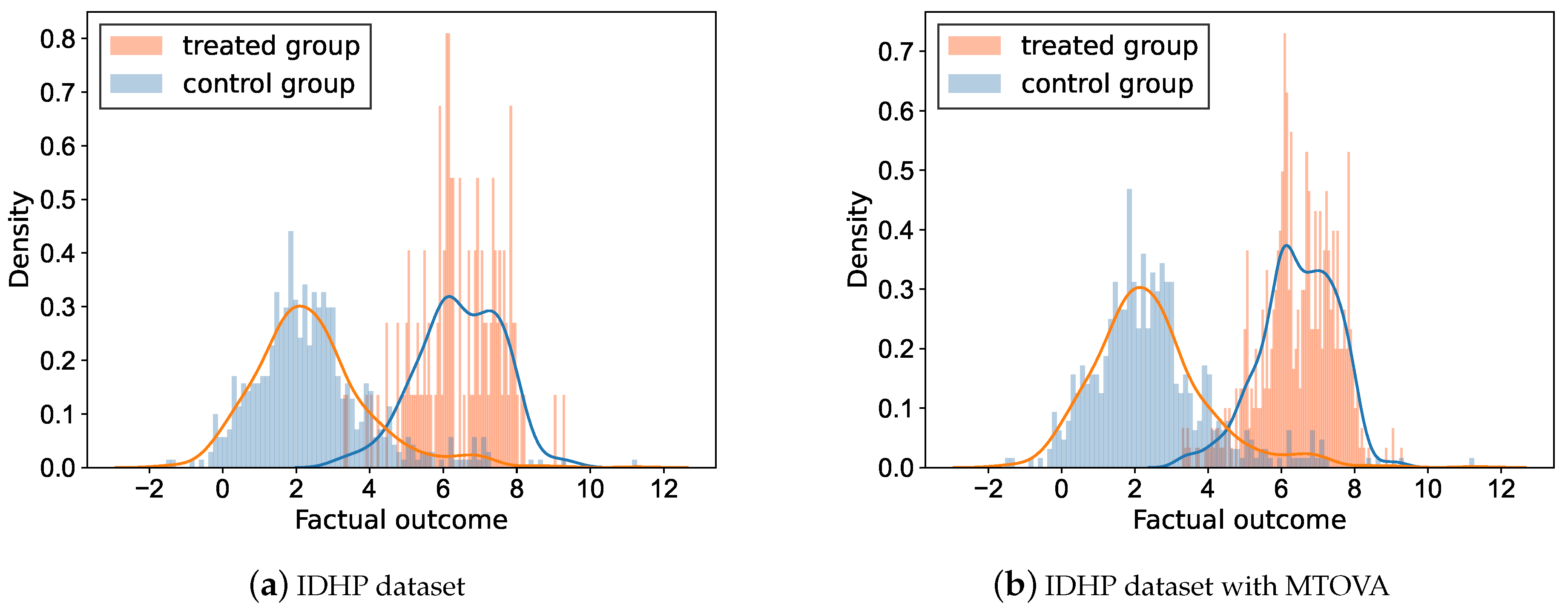
We illustrate the impact of DTGS with an example. Employing the subset of IDHP dataset [23] containing 547 control samples and 125 treated samples, we plot the frequency histogram of the factual outcome for the different treatment groups in this dataset in Figure 1a. We can see that the frequency histogram of factual outcomes for the treated group with the smaller sample size has significant missing values for certain regions compared to the control group. We have the intuition that the absence of factual outcome is largely accompanied by the absence of features, i.e., some samples have not yet been observed, which is most likely caused by treatment selection bias. From the experience of extensive machine learning, the smaller the sample size, the lower the accuracy tends to be. Therefore, we speculate that DTGS will affect the above predictive accuracy of factual outcomes.

In addition, the other intuition is that the imbalanced variance between the treated and control groups also affects the performance of estimating ITE. As shown in Figure 1b, the kernel density curve of the treated group is wider compared to the control group. Corollary 1 confirms the above intuition.

Therefore, we consider expanding the minority group to minimize the effect of missing data and large variance differences due to treatment selection bias.

Given the impact of DTGS for estimating ITE, we propose two simple yet effective methods: Minority in Treatment Over-sampling (MTOVA) and Factual Outcome Distribution Smoothing (FODS). We combine these two methods with some current frameworks for estimating ITE for addressing DTGS.

2.4. Methods

2.4.1. Frameworks for Estimating ITE

Grounded on or inspired by Theorem 2, numerous methods based on deep representation learning are proposed to solve the above two major challenges and outperform the state-of-the-art [13,16]. The ideas of such methods are similar but the optimization objectives are different.

Let $f:\mathcal{X}\times \{0,1\}\to \mathcal{Y}$ by a hypothesis, such that $f(x,t):=h\left(\mathsf{\Phi }\right(x),t)$ for a representation $\mathsf{\Phi }$ defined over $\mathcal{X}$ and hypothesis h defined over the output of $\mathsf{\Phi }:\mathcal{X}\to \mathcal{R}$. CFR uses the following objective, minimizing the ITE error upper bond and parameterizing $\mathsf{\Phi }\left(x\right)$ and $h\left(\mathsf{\Phi }\right(x),t)$ by deep neural networks trained jointly:

$$\begin{array}{cc}\hfill \underset{\genfrac{}{}{0pt}{}{h,\mathsf{\Phi }}{\parallel \mathsf{\Phi }\parallel =1}}{min}& \frac{1}{n}\sum _{i=1}^n{w}_i·L(h(\mathsf{\Phi }\left(x_i\right),t_i),Y_i)+\lambda ·\mathfrak{R}\left(h\right)\hfill \\ \hfill & +\alpha ·{\mathrm{IPM}}_{\mathrm{G}}\left({\left\{\mathsf{\Phi }\left(x_i\right)\right\}}_{i:t_i=0}\right),{\left\{\mathsf{\Phi }\left(x_i\right)\right\}}_{i:t_i=1}),\hfill \end{array}$$

(13)

where L is a square loss function and $\mathfrak{R}$ is a model complexity term. ${\mathrm{IPM}}_{\mathrm{G}}$ is a measure of the distance between the control and treated group distributions (empirical) in the representation space [24]. For two probability density functions $p,q$ defined over $U\subseteq {\mathbb{R}}^d$ and function family G of functions g: $U\to \mathbb{R}$, ${\mathrm{IPM}}_{\mathrm{G}}:=\underset{g\in G}{sup}\left|{\int }_{u}g\left(u\right)(p\left(u\right)-q\left(u\right))du\right|$.

The objective function of feature selection representation matching (FSRM) model is slightly different and is simply illustrated as follows:

$$\begin{array}{cc}\hfill min& -\frac{1}{n}\sum _{i=1}^n\sum _{j=1}^K\left(t_{ij}log\left({\widehat{t}}_{ij}\right)\right)\hfill \\ \hfill & +\frac{1}{n}\sum _{i=1}^n{w}_i·L({\widehat{Y}}_i^{t_i},Y_i)\hfill \\ \hfill & +\alpha ·IP{M}_{WASS}\hfill \\ \hfill & +\lambda ·{\mathfrak{R}}_{LASSO}\hfill \\ \hfill & +\beta ·\mathfrak{R}.\hfill \end{array}$$

(14)

The first term in Equation (14) above is the loss function for factual treatment assignment prediction. The second and third terms, respectively, correspond to the same first and third terms in the CFR objective function. The fourth term is an elastic net term based on LASSO [25], used for deep feature selection and regularization. The last term regularizes the deep prediction network.

We propose two techniques that can easily be integrated into such frameworks, ensuring the error of estimating $\tau \left(x\right)=m_1\left(x\right)-m_0\left(0\right)$ that is as small as possible and has good out-of-sample performance in the DTGS task.

2.4.2. Minority in Treatment Over-Sampling

Based on the above analyses of the impact of DTGS, we argue that a data-based solution should have the following performances.

• Able to expand minority samples: The “head” of predicting the factual outcome of the minority is often poorly generalized in DTGS, resulting in a larger prediction error on the test set.
• Able to compensate for potential missing data: If the sample size of a treatment group is small, the sample distribution tends to be sparse even after characterization $\mathsf{\Phi }$. In other words, the value space of ${\left\{\mathsf{\Phi }\left(x_i\right)\right\}}_{i:t_i=0}$ and ${\left\{\mathsf{\Phi }\left(x_i\right)\right\}}_{i:t_i=1}$ is extremely different, seeing the t-SNE visualization of the representation of the IHDP learned by ${\mathrm{CFR}}_{\mathrm{MMD}}$ (Figure 2b). In this case, according to Equation (13), it is difficult to find a satisfactory $\mathsf{\Phi }$, which makes the $p_{\mathsf{\Phi }}^{t=1}\left(r\right)$ (empirical) and $p_{\mathsf{\Phi }}^{t=0}\left(r\right)$ (empirical) similar. Therefore, the method ought to compensate for potential missing by identifying similar but more specific regions in the feature space.
• Able to achieve variance approximation: According to Corollary 1, the upper bound is smallest when ${\sigma }_{Y_0}^2$ and ${\sigma }_{Y_1}^2$ are close.

Figure 2. t-SNE visualizations of IHDP: (a) the distribution of original data; (b) the balanced representation of IHDP learned by CFR Wass; (c) the balanced representation of IHDP learned by CFR Wass using MTOVA.

Figure 2. t-SNE visualizations of IHDP: (a) the distribution of original data; (b) the balanced representation of IHDP learned by CFR Wass; (c) the balanced representation of IHDP learned by CFR Wass using MTOVA.

A brace of algorithms has been developed to learn from imbalanced datasets in machine learning [19,20]. However, these methods are slightly different from the context of this paper. The goal of our task is to learn the $\mathsf{\Phi }\left(x\right)$ and $h\left(\mathsf{\Phi }\right(x),t)$ such that the ${ϵ}_{\mathrm{PEHE}}$ is small.

Inspired by the Synthetic Minority Over-sampling Technique (SMOTE), we apply the idea of over-sampling the minority group to solve the first conjecture and second conjecture above. To satisfy the third point, we present the variance approximation theorem.

Theorem 3 (Variance approximation).

Two samples, $y_1$ and $y_2$, are randomly sampled from the one-dimensional random variable Y, with the current sample variance $Va{r}_1$. A point $y_3$ is randomly selected as a new sample point on the line connecting $y_1$ and $y_2$, i.e., $y_3=\lambda y_1+(1-\lambda )y_2$ with $\lambda \in (0,1)$. The current sample variance is $Va{r}_2$. We have $Va{r}_2\le Va{r}_1$.

Proof. 

The proof process is shown as Theorem A1 in Appendix A.    □

According to Theorem 3, the variance of the three points is less than that of the original two points after randomly synthesizing new samples on the line connecting the two points. Since there is no guarantee that the variance of all the samples after synthesizing the sample points will be less than that before synthesizing, we can add a variance filtering mechanism.

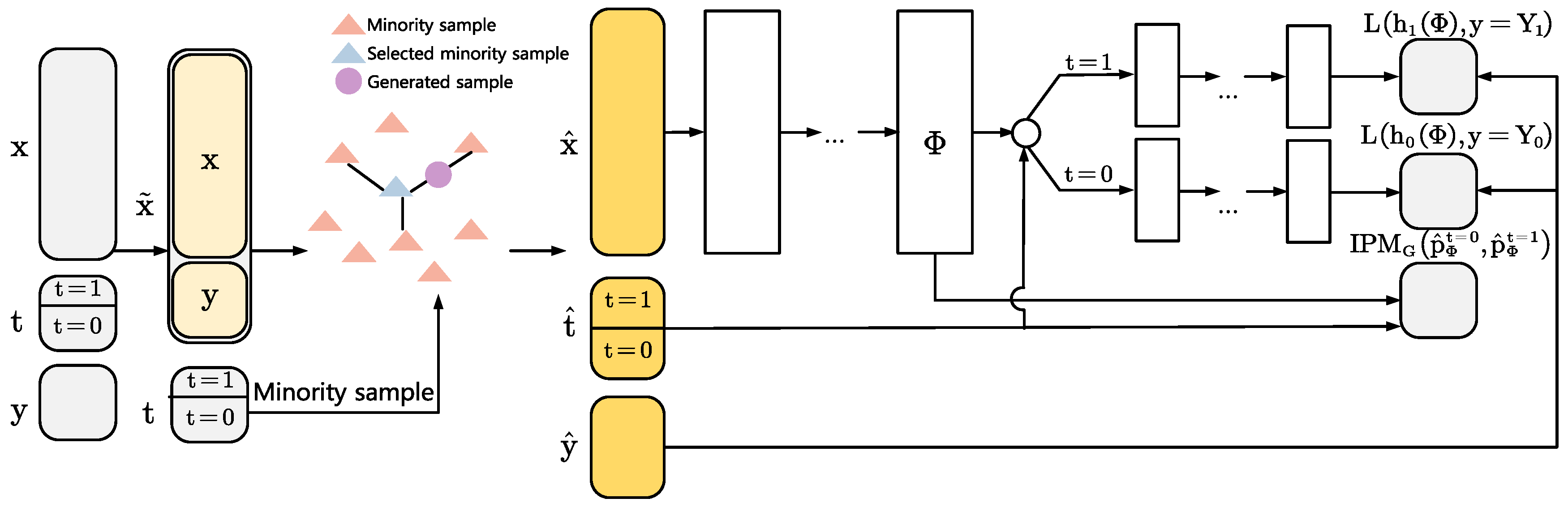
In general, the variance tends to be larger for the minority group, as shown in Figure 1a. Therefore, the minority in treatment over-sampling based on variance approximation (MTOVA) is proposed that both over-samples the minority group and allows the variance of the minority group to constantly approximate another group. The pseudo-code for MTOVA is shown in Algorithm 1. We can easily embed the MTOVA into the framework for estimating ITE, such as the CFR framework, as shown in Figure 3.

Algorithm 1 MTOVA: Minority in Treatment Over-Sampling based on Variance Approximation
1:	Input: Original majority group samples ${\mathcal{D}}_1={\left\{({\mathbf{x}}_i,t_i,y_i)\right\}}_{i=1}^M$; Original minority group samples ${\mathcal{D}}_2={\left\{({\mathbf{x}}_j,t_j,y_j)\right\}}_{j=1}^N$; The set of synthetic sample ${\mathcal{D}}_3$
2:	Calculate the variance $Va{r}_1$ of the majority group ${\mathcal{D}}_1$
3:	Calculate the variance $Va{r}_2$ of the minority group ${\mathcal{D}}_2$
4:	while $M-N\ne 0$ and $Va{r}_1\le Va{r}_2$ do
5:	for i to N do
6:	Choose existing methods to synthesize a new sample j
7:	Calculate the variance $Va{r}_{new}$ of ${\mathcal{D}}_2=\{{\mathcal{D}}_2\cup j\}$
8:	if $Va{r}_{new}\le Va{r}_2$ then
9:	Add j to the set of synthetic sample ${\mathcal{D}}_3$
10:	${\mathcal{D}}_2=\{{\mathcal{D}}_2\cup {\mathcal{D}}_3\}$
11:	$Va{r}_2=Va{r}_{new}$
12:	$N=N+1$
13:	else
14:	break
15:	end if
16:	end for
17:	end while

For the IDHP example, frequency histograms of the factual outcome and t-SNE visualization of the representation using the MTOVA for the control and treated groups are also plotted, as jointly shown in Figure 1b and Figure 2c. Figure 1b illustrates that the potentially missing parts of the frequency histogram of the factual outcome of the treated group after using MTOVA are somewhat filled in. Figure 2c shows that the distribution of control and treated groups on the representation space changed significantly after using MTOVA. We see this change as a move towards better reflecting the overall distribution $p_{\mathsf{\Phi }}\left(r\right)$ in representation $\mathsf{\Phi }$ space.

2.4.3. Factual Outcome Distribution Smoothing

We submit an additional solution for DTGS from the point of view of algorithmic improvement in this section.

In the CFR framework, the inverse of the proportion of the control and treated group sample sizes to the total sample size as their respective compensation factors are utilized to calibrate for the DTGS task. The compensation factor is $w_i=\frac{t_i}{2u}+\frac{1-t_i}{2(1-u)}$ in Equation (13), where $u=\frac{1}{n}{\sum }_{i=1}^n{t}_i$, lacking processing of potential missing data within the two treatment groups, which is undoubtedly crude.

Confounding factors often make $p^{t=1}\left(x\right)$ and $p^{t=0}\left(x\right)$ different and may both differ significantly from the $p\left(x\right)$ in the overall population. It can be inferred that the distribution of the control and treated groups will also significantly differ from the distribution of $Y_0$ and $Y_1$ in the overall population. Therefore, we attempt to adjust the weights $w_i$ for the prediction error component of Equation (13) such that both the prediction error and $IPM$ could be reduced. To ensure the learned hypothesis $f:\mathcal{X}\times \{0,1\}\to \mathcal{Y}$ to able to deal with potential missing data, we try to seek an efficient density estimator of the factual outcome to calibration for the prediction loss.

At present, a non-parametric estimation method has been widely used in statistics for probability density estimation, i.e., kernel density estimation. The Factual Outcome Distribution Smoothing (FODS) proposed in this paper is based on the kernel density estimation of $Y_0$ and $Y_1$ [21], convolving a symmetric kernel with the empirical density distribution of a continuous label.

The label space is divided into n groups with the same group distance, forming the following grouping intervals $[y_0,y_1),\dots ,[y_{(n-1)},y_n)$, using $N=\{1,2,\dots n\}\subset {\mathbb{Z}}^{+}$ to denote the indexes of the above intervals. $p\left(y\right)$ is the number of training sets contained in the interval, where y is located, i.e., the empirical label density. $\tilde{p}\left(y^{\prime }\right)$ is the effective label density of label $y^{\prime }$, and $k(y,y^{\prime })$ is a symmetric kernel. $\tilde{p}\left(y^{\prime }\right)$ is the effective label density for y, as follows:

$$\tilde{p}\left(y^{\prime }\right)\triangleq {\int }_{\mathcal{Y}}\mathrm{k}(y,y^{\prime })p\left(y\right)dy.$$

(15)

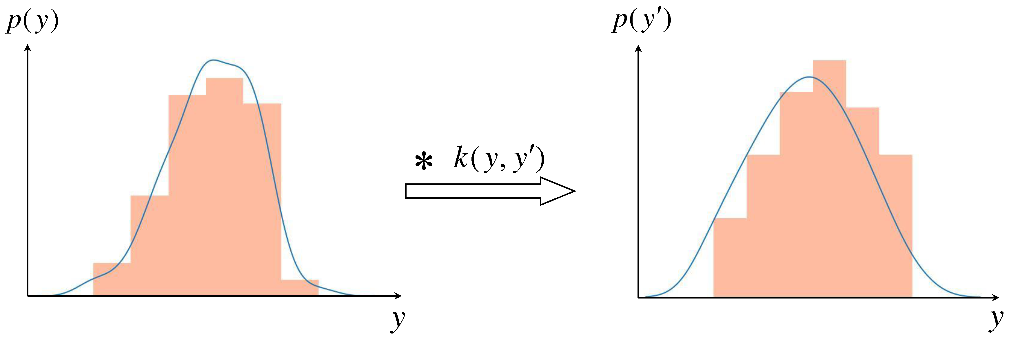
We believe that the effective label density is smoother compared to the empirical label density when the sample better reflects the overall characteristics, see Figure 4. We can integrate the effective density estimate $\tilde{p}\left(y^{\prime }\right)$ of the factual outcome into the general frameworks for estimating ITE in DTGS, such as CFR, see Algorithm 2.

The method successfully reduces the impact of DTGS by correcting for sample size imbalance within and between the treated and control groups by $w_i$ in Equation (13).

Algorithm 2 CFR-FODS: Counterfactual Regression with Factual Outcome Distribution Smoothing
1:	Input: Factual sample $\mathcal{D}={\left\{({\mathbf{x}}_i,t_i,y_i)\right\}}_{i=1}^n$, scaling parameter $\alpha >0$, loss function L, representation network ${\mathsf{\Phi }}_{\mathbf{W}}$ with initial weights $\mathbf{W}$, outcome network $h_{\mathbf{V}}$ with initial weights $\mathbf{V}$, function family G for IPM, bin size $\Delta b$, symmetric kernel distribution $k(y,y^{\prime })$
2:	Calculate $u=\frac{1}{n}{\sum }_{i=1}^n{t}_i$
3:	Calculate $c_i=\frac{t_i}{2u}+\frac{1-t_i}{2(1-u)}$
4:	Calculate the empirical label density distribution $p\left(y\right)$ based on $\Delta b$ and $\mathcal{D}$
5:	Calculate the effective label density distribution $\tilde{p}\left(y\right)\triangleq {\int }_{\mathcal{Y}}\mathrm{k}(y,y^{\prime })p\left(y\right)dy$
6:	for all$({\mathbf{x}}_i,t_i,y_i)\in \mathcal{D}$  do
7:	Calculate the $w_i=\frac{c_i}{\tilde{p}\left(y_i\right)}\propto \frac{1}{\tilde{p}\left(y_i\right)}$
8:	end for
9:	while not converged do
10:	Sample mini-batch ${\left\{({\mathbf{x}}_i,t_i,y_i,w_i)\right\}}_{i=1}^m$ from $\mathcal{D}$
11:	Calculate the gradient of the IPM term:
12:	$g_1={\nabla }_{\mathbf{W}}IP{M}_G({\left\{\mathsf{\Phi }\left(x_i\right)\right\}}_{i:t_i=0},{\left\{\mathsf{\Phi }\left(x_i\right)\right\}}_{i:t_i=1})$
13:	Calculate the gradients of the empirical loss:
14:	$g_2={\nabla }_{\mathbf{V}}\frac{1}{m}{\sum }_j{w}_{i_j}L(h_{\mathbf{V}}({\mathsf{\Phi }}_{\mathbf{W}}\left(x_{i_j}\right),t_{i_j}),y_i)$
15:	$g_3={\nabla }_{\mathbf{W}}\frac{1}{m}{\sum }_j{w}_{i_j}L(h_{\mathbf{V}}({\mathsf{\Phi }}_{\mathbf{W}}\left(x_{i_j}\right),t_{i_j}),y_i)$
16:	Obtain step size scalar or matrix $\eta$ with standard neural net methods
17:	$[\mathbf{W},\mathbf{V}]\leftarrow [\mathbf{W}-\eta (\alpha g_1+g_3),\mathbf{V}-\eta (g_2+2\lambda \mathbf{V})]$
18:	Check convergence criterion
19:	end while

3. Experiment

3.1. Datasets

Causal inference algorithms are much more challenging than many machine learning tasks in the choice of dataset and evaluation criteria, as we never access real ITE from the data. We chose two benchmark datasets in the current causal inference community: a semi-synthetic dataset [23] and a real-world dataset from the Job Corps randomized controlled trial (RCT) in the USA [26]. By non-randomly removing a biased subset of the two datasets for a given treatment group, we obtained the datasets suitable for the context targeted by our method, i.e., the experimental datasets have different distributions and sample sizes for both the control and treated groups.

3.1.1. Simulations Based on Real Data: IHDP

The IHDP dataset collected from the Infant Health and Development Program (IHDP) is commonly used to estimate causal effects. The dataset is from a randomized controlled trial that obtains a set of 25 covariates reflecting the characteristics of newborns and their mothers, containing 6 continuous covariates and 19 binary covariates. The outcome of such a dataset is the infants’ cognitive test scores. Both factual and counterfactual outcomes can be simulated through the NPCI package [27].

We generated 1000 equally sized subsets of the IHDP dataset. Every subset contains 747 units, including 608 control units and 139 treated units. The sample size ratio between the treated and control groups in these 1000 datasets is around 1:4, which belongs to DTGS. We conduct experiments using 1000 datasets with a treated group ratio of approximately 0.2 and 63/27/10 for training/validation/test splits. We ensure that the training and the validation sets have no observed sample in the testing set and report the results of the testing set.

3.1.2. Real-World Data: JC

The US Job Corps Experiment dataset, which contains information on weekly earnings, criminal activity rates, and other information for disadvantaged youth who meet the criteria and are randomly assigned to participate in the Job Corps Experiment over time, is used to explore social issues such as the impact of educational attainment on employment, earnings, and violent crime rates. The dataset has 9240 observations and 46 independent variables. In the experiments in this paper, we assess the individual causal effect of the Job Corps experiment’s random assignment scheme on weekly earnings in the fourth year after assignment, selecting the 28 descriptive variables before the start of the assignment scheme as background characteristics of the sample, and treating those randomly assigned into Job Corps as the treated group and otherwise as the control group.

We artificially generate differences in treatment group distributions and sample sizes by removing a biased subset of the control population on the set of continuous covariates. We construct 100 datasets (800 units, 28 covariates) for the experiment, with a treated group ratio of approximately 0.85 satisfying DTGS and 63/27/10 for training/validation/test splits.

3.2. Baseline

We compare our two methods with the following baseline methods:

Balancing linear regression (BLR) learns a relatively balanced representation space by limiting the influence of imbalanced features on the prediction of the outcomes. BLR binds the relative error of fitting a ridge-regression using the distribution with reverse treatment assignment versus fitting a ridge-regression using the factual distribution. Unfortunately, such a bound is not at all informative regarding the ${ϵ}_{\mathrm{PEHE}}$ [28].

Counterfactual regression (CFR) controls confounding factors and obtains counterfactual outcomes on a new representation space, using the ideas of deep representation and domain adaptation [15]. Compared to BLR, CFR provides an informative bound on the absolute quality of the representation. The CFR is specifically divided into ${\mathrm{CFR}}_{\mathrm{MMD}}$ and ${\mathrm{CFR}}_{\mathrm{WASS}}$, which depends on the form of IPMs, such as the Wasserstein and MMD distances.

Treatment-agnostic representation network (TARNET) is a special case of CFR, whose variant without balancing regularization, i.e., ${\mathrm{IPM}}_{\mathrm{G}}=0$ in Equation (13) [15].

Feature selection representation matching (FSRM) model maps the original feature space into a selective, nonlinear, and balanced representation space, and then conducts matching in the learned representation space [16].

3.3. Metric

For simulation datasets that contain counterfactual outcomes such as the IHDP dataset, we report the PEHE loss, i.e., Equation (8) and we give a finite sample form, as follows:

$$\begin{array}{c}\hfill {\widehat{ϵ}}_{\mathrm{PEHE}}\left(f\right)=\frac{1}{n}\sum _{i=1}^n{({\tau }_f\left(x_i\right)-{\widehat{\tau }}_f\left(x_i\right))}^2,\end{array}$$

(16)

However, for real-world data, the counterfactual outcome cannot be observed, only the nearest-neighbor approximation of PEHE loss (Equation (8)) can be taken as a measure, such as the real JC dataset. In this case, we use the nearest-neighbor approximation of the PEHE loss, which is:

$${\widehat{ϵ}}_{{\mathrm{PEHE}}_{\mathrm{nn}}}\left(f\right)=\frac{1}{n}\sum _{i=1}^n(1-2t_i){((y_{j\left(i\right)}-y_i)-{\widehat{\tau }}_f\left(x_i\right))}^2,$$

(17)

where $y_{j\left(i\right)}$, as the surrogate for the counterfactual outcome, is the observed outcome of the nearest neighbor $j\left(i\right)$ to i in the opposite treatment group with $t_{j\left(i\right)}=1-t_i$.

4. Results

The performances that the MTOVA and FODS integrate with the above baseline models for estimating ITE on the test set of the two datasets are reported in

Table 1. Results on IHDP and JC. Lower is better.

	IDHP		JC
Metrics	$\sqrt{{\mathbf{ϵ}}_{\mathbf{PEHE}}}$	$\sqrt{{\mathbf{ϵ}}_{{\mathbf{PEHE}}_{\mathbf{nn}}}}$	$\sqrt{{\mathbf{ϵ}}_{{\mathbf{PEHE}}_{\mathbf{nn}}}}$
$\mathrm{BLR}$	2.82 ± 0.12	5.74 ± 0.23	283.45 ± 8.15
$\mathrm{BLR}+\mathrm{MTOVA}$	2.59 ± 0.10	5.61 ± 0.22	271.18 ± 7.23
$\mathrm{BLR}+\mathrm{FODS}$	2.43 ± 0.10	5.55 ± 0.21	269.26 ± 7.29
$\mathrm{TARNET}$	1.64 ± 0.03	5.69 ± 0.23	269.82 ± 7.30
$\mathrm{TARNET}+\mathrm{MTOVA}$	1.33 ± 0.07	5.52 ± 0.22	267.13 ± 6.63
$\mathrm{TARNET}+\mathrm{FODS}$	1.60 ± 0.07	5.35 ± 0.21	279.22 ± 7.31
${\mathrm{CFR}}_{\mathrm{MMD}}$	1.42 ± 0.03	5.62 ± 0.22	275.42 ± 7.13
${\mathrm{CFR}}_{\mathrm{MMD}}+\mathrm{MTOVA}$	1.10 ± 0.06	5.48 ± 0.22	267.18 ± 6.63
${\mathrm{CFR}}_{\mathrm{MMD}}+\mathrm{FODS}$	0.90 ± 0.03	5.50 ± 0.22	264.32 ± 10.19
${\mathrm{CFR}}_{\mathrm{WASS}}$	1.11 ± 0.02	5.66 ± 0.23	275.58 ± 6.71
${\mathrm{CFR}}_{\mathrm{WASS}}+\mathrm{MTOVA}$	0.95 ± 0.00	5.62 ± 0.23	267.09 ± 6.64
${\mathrm{CFR}}_{\mathrm{WASS}}+\mathrm{FODS}$	0.79 ± 0.03	5.47 ± 0.22	263.19 ± 7.22
$\mathrm{FSRM}$	1.24 ± 0.04	5.67 ± 0.23	275.82 ± 6.98
$\mathrm{FSRM}+\mathrm{MTOVA}$	1.02 ± 0.03	5.58 ± 0.22	265.09 ± 6.78
$\mathrm{FSRM}+\mathrm{FODS}$	0.85 ± 0.02	5.42 ± 0.22	262.89 ± 7.02

. The results in the table contain the mean and standard errors of the results of multiple replicated trials.

We use Adam [29] to parameterize parameters in every baseline models, such as $\mathsf{\Phi }\left(x\right)$ and $h\left(\mathsf{\Phi }\right(x),t)$ in CFR and $\mathsf{\Phi }\left(x\right)$, $h_1(\mathsf{\Phi }\left(x\right),t)$, and $h_2(\mathsf{\Phi }\left(x\right),t)$ in FSRM. In MOTVA, since the experimental datasets have both continuous and categorical variables, we chose the existing SMOTENC to implement the over-sampling procedure. We combine FODS with the loss inverse re-weighting scheme in the optimization objective of such baselines for estimating ITE. The example details of hyperparameters in CFR-FODS are shown in

Table 2. Hyperparameters and ranges in CFR-FODS.

Parameter	Range
Kernel	{gaussian, laplace}
Kernel size(odd number)	{1, 3, 5, 7, 9}
Kernel parameter, $\sigma$	${\left\{0.5k\right\}}_{k=1}^{10}$
reweight	{inverse, sqrt inverse}
Imbalance parameter, $\alpha$	${\{3\times {10}^k\}}_{k=-3}^2$
regularization parameter, $\lambda$	${\left\{{10}^k\right\}}_{k=-4}^2$
Num. representation layers	{1, 2, 3}
Num. hypothesis layers	{1, 2, 3}
Dim. representation layers	{100, 200}
Dim. hypothesis layers	{100, 200}
Batch size	{100, 200, 500}

.

5. Discussion

The evaluation metrics of both the IDHP dataset and the JC dataset perform better relative to the baseline models themselves after applying our techniques. To interpret these results, we perform a parametric analysis and visualization based on the effects of combining the two techniques and the CFR framework.

5.1. Discussion of MTOVA

By comparing the expected variance of $Y_t$ in Equation (9) before and after using MTOVA, we find that MTOVA does indeed bring ${\sigma }_{Y_0}^2$ and ${\sigma }_{Y_1}^2$ closer together, as shown in Figure A2. We calculate that the prediction loss of CFR-MTOVA on the validation set, i.e., $L(h((\mathsf{\Phi }\left(x_i\right),t),Y_i)$ in Equation (13), is smaller than CFR. Such results verify our intuitions in Section 2.4.2.

5.2. Discussion of FODS

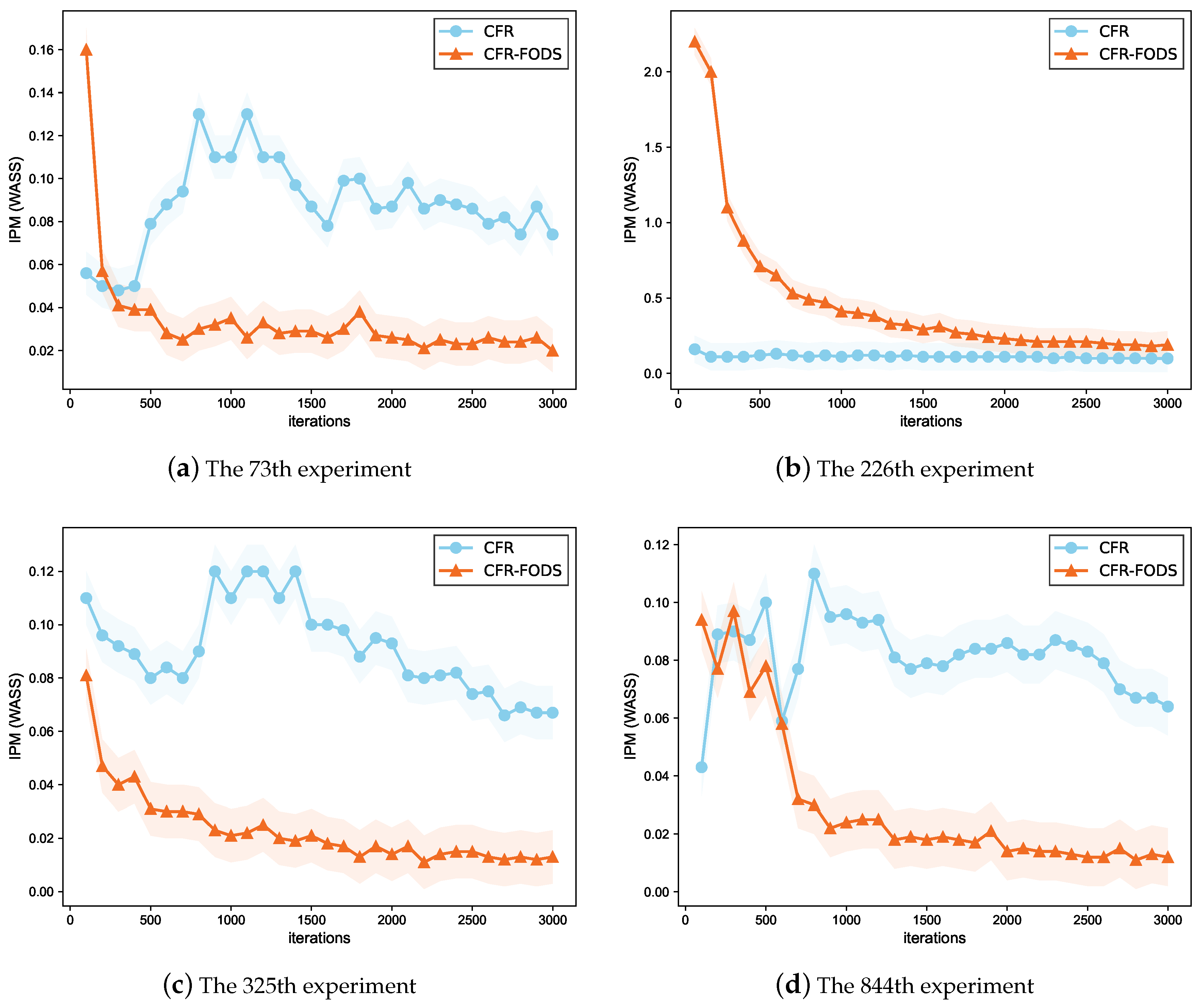
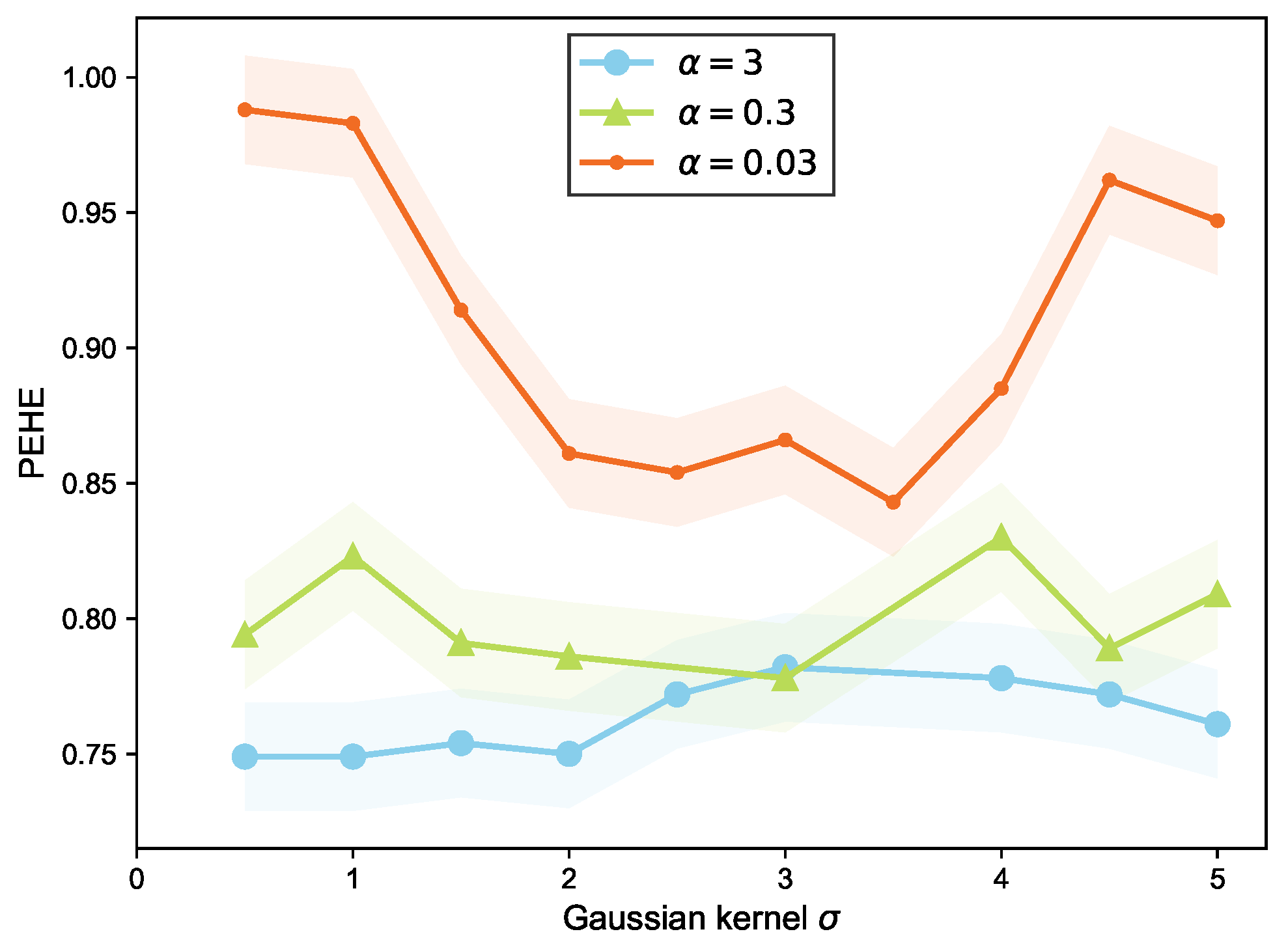
By searching for the optimal hyperparameters kernel size and $\sigma$ of the FODS Gaussian kernel function, we find that FODS is sensitive to the values of the two hyperparameters of the kernel function. The optimal value of the key hyperparameter $\alpha$ in the CFRNET varies for different kernel sizes and $\sigma$, as shown in Figure A1. This verifies our inference that FODS affects both the prediction error and the IPM term in Equation (13). Figure 5 illustrates that the CFR-FODS can quickly reduce the IPM and that the IPM at the end of model training is smaller compared to CFR.

More importantly, the distribution (empirical) of control and treated groups over the representation space at this point is more reflective of the overall distribution. Therefore, the trained model performs well out-of-sample, as shown in

Table A1. Within-sample and out-of-sample results on IHDP based on FODS. Lower is better.

	Within-Sample		Out-of-Sample
Metrics	$\sqrt{{\mathbf{ϵ}}_{\mathbf{PEHE}}}$	$\sqrt{{\mathbf{ϵ}}_{{\mathbf{PEHE}}_{\mathbf{nn}}}}$	$\sqrt{{\mathbf{ϵ}}_{\mathbf{PEHE}}}$	$\sqrt{{\mathbf{ϵ}}_{{\mathbf{PEHE}}_{\mathbf{nn}}}}$
$\mathrm{TARNET}$	1.67 ± 0.03	5.47 ± 0.21	1.64 ± 0.03	5.69 ± 0.23
$\mathrm{TARNET}+\mathrm{FODS}$	1.62 ± 0.07	5.16 ± 0.20	1.60 ± 0.07	5.35 ± 0.21
${\mathrm{CFR}}_{\mathrm{MMD}}$	1.27 ± 0.04	5.54 ± 0.21	1.42 ± 0.03	5.52 ± 0.22
${\mathrm{CFR}}_{\mathrm{MMD}}+\mathrm{FODS}$	0.95 ± 0.05	5.34 ± 0.22	0.90 ± 0.03	5.50 ± 0.22
${\mathrm{CFR}}_{\mathrm{WASS}}$	1.15 ± 0.02	5.49 ± 0.22	1.11 ± 0.02	5.66 ± 0.23
${\mathrm{CFR}}_{\mathrm{WASS}}+\mathrm{FODS}$	0.87 ± 0.06	5.28 ± 0.28	0.79 ± 0.03	5.47 ± 0.22

, which is robust.

Based on the effects of TARNET whose optimization objective does not include the IPM term in combination with the two methods, we are more confident that FODS affects both the predicted loss term and the IPM term in Equation (13).

5.3. Comparison of MTOVA and FODS

Comparing the two methods, FODS performs better with the CFR framework and best with ${\mathrm{CFR}}_{\mathrm{WASS}}$. This is mainly because, in the MTOVA method, we only synthesize new samples for the minority group, while the sample distribution in another group may also be sparse. However, in the FODS method, we not only take into account differences in sample size between treatment group groups, but also deal with imbalances in the continuous potential outcome within each treatment group.

6. Conclusions and Future Work

We naturally introduced the DTGS-CFR task based on the CFR framework, i.e., learning individual causal effect estimators from a dataset with imbalanced sample sizes in the treated and control groups. We propose two different perspectives, CFR-MTOVA and CFR-FODS, to eliminate the effects of this sample size imbalance. Of these, CFR-FODS stands out both in the IDHP dataset and the JC dataset. Although CFR-MTOVA is not as state-of-the-art as CFR-FODS, CFR-MTOVA also performs significantly better than CFR in the DTGS-CFR context and provides us with many open questions for discussion.

In the future, we can consider exploring the following directions:

1.

According to the studies on the problem of classifying unbalanced datasets [30,31], we can discuss whether the treatment group with the larger sample needs to be treated as well in MTOVA;

2.

There has been a lot of interest in applying machine learning methods, e.g., supervised learning methods such as random forests and neural networks, to causal effect inference, known as causal machine learning (CML) [32]. We can further discuss the effect of combining the two techniques with other CML methods, such as causal forests (CF);

3.

How our two methods affect ITE estimates for samples with different levels of imbalance between treated and control groups.

References

- Knaus, M.C. A double machine learning approach to estimate the effects of musical practice on student’s skills. J. R. Stat. Soc. Ser. A Stat. Soc. 2021, 184, 282–300. [Google Scholar] [CrossRef]
- Poulos, J.; Zeng, S. RNN-based counterfactual prediction, with an application to homestead policy and public schooling. J. R. Stat. Soc. Ser. C Appl. Stat. 2021, 70, 1124–1139. [Google Scholar] [CrossRef]
- Knaus, M.C. Double machine learning-based programme evaluation under unconfoundedness. Econom. J. 2022, 25, 602–627. [Google Scholar] [CrossRef]
- Schuler, A.; Baiocchi, M.; Tibshirani, R.; Shah, N. A comparison of methods for model selection when estimating individual treatment effects. arXiv 2018, arXiv:1804.05146. [Google Scholar]
- Schwab, P.; Linhardt, L.; Bauer, S.; Buhmann, J.M.; Karlen, W. Learning counterfactual representations for estimating individual dose–response curves. In Proceedings of the AAAI Conference on Artificial Intelligence, New York, NY, USA, 7–12 February 2020. [Google Scholar]
- Rubin, D.B. Estimating causal effects of treatments in randomized and nonrandomized studies. J. Educ. Psychol. 1974, 66, 688–701. [Google Scholar] [CrossRef]
- Splawa-Neyman, J.; Dabrowska, D.M.; Speed, T.P. On the application of probability theory to agricultural experiments. Essay on principles. Section 9. Stat. Sci. 1990, 5, 465–472. [Google Scholar] [CrossRef]
- Pearl, J. Causality; Cambridge University Press: Cambridge, UK, 2009. [Google Scholar]
- Fisher, R.A. The Design of Experiments; Hafner Press, A Division of Macmillan Publishing Co., Inc.: New York, NY, USA; Collier Macmillan Publishers: London, UK, 1960. [Google Scholar]
- Cochran, W.G.; Chambers, S.P. The planning of observational studies of human populations. J. R. Stat. Soc. A Gen. 1965, 128, 234–266. [Google Scholar] [CrossRef]
- Yule, G.U. Notes on the theory of association of attributes in statistics. Biometrika 1903, 2, 121–134. [Google Scholar] [CrossRef]
- Simpson, E.H. The interpretation of interaction in contingency tables. J. R. Stat. Soc. Ser. B Methodol. 1951, 13, 238–241. [Google Scholar] [CrossRef]
- Shalit, U.; Johansson, F.D.; Sontag, D. Estimating individual treatment effect: Generalization bounds and algorithms. In Proceedings of the 34th International Conference on Machine Learning, Sydney, Australia, 6–11 August 2017. [Google Scholar]
- Ben-David, S.; Blitzer, J.; Crammer, K.; Kulesza, A.; Pereira, F.; Vaughan, J.W. A theory of learning from different domains. Mach. Learn. 2010, 79, 151–175. [Google Scholar] [CrossRef]
- Ganin, Y.; Ustinova, E.; Ajakan, H.; Germain, P.; Larochelle, H.; Laviolette, F.; Lempitsky, V. Domain-adversarial training of neural networks. J. Mach. Learn. Res. 2016, 17, 1–35. [Google Scholar]
- Chu, Z.; Rathbun, S.L.; Li, S. Matching in selective and balanced representation space for treatment effects estimation. In Proceedings of the 29th ACM International Conference on Information & Knowledge Management, New York, NY, USA, 19–23 October 2020. [Google Scholar]
- Zhang, Y.; Alexis, B.; Mihaela, S. Learning overlapping representations for the estimation of individualized treatment effects. In Proceedings of the 23rd International Conference on Artificial Intelligence and Statistics, Palermo, Italy, 26–28 August 2020. [Google Scholar]
- Poulos, J.; Horvitz-Lennon, M.; Zelevinsky, K.; Cristea-Platon, T.; Huijskens, T.; Tyagi, P.; Normand, S.L. Targeted Learning in Observational Studies with Multi-Valued Treatments: An Evaluation of Antipsychotic Drug Treatment Safety. Stat. Med. 2024, 43, 1489–1508. [Google Scholar] [CrossRef] [PubMed]
- Chawla, N.V.; Bowyer, K.W.; Hall, L.O.; Kegelmeyer, W.P. SMOTE: Synthetic minority over-sampling technique. J. Artif. Intell. Res. 2002, 16, 321–357. [Google Scholar] [CrossRef]
- Torgo, L.; Branco, P.; Ribeiro, R.P.; Pfahringer, B. Resampling strategies for regression. Expert Syst. 2015, 32, 465–476. [Google Scholar] [CrossRef]
- Yang, Y.; Zha, K.; Chen, Y.; Wang, H.; Katabi, D. Delving into deep imbalanced regression. In Proceedings of the 38th International Conference on Machine Learning, Vienna, Austria, 18–24 July 2021. [Google Scholar]
- Rosenbaum, P.R.; Rubin, D.B. The central role of the propensity score in observational studies for causal effects. Biometrika 1983, 70, 41–55. [Google Scholar] [CrossRef]
- Hill, J.L. Bayesian nonparametric modeling for causal inference. J. Comput. Graph. Stat. 2011, 20, 217–240. [Google Scholar] [CrossRef]
- Sriperumbudur, B.K.; Fukumizu, K.; Gretton, A.; Schölkopf, B.; Lanckriet, G.R. On the empirical estimation of integral probability metrics. Electron. J. Stat. 2012, 6, 1550–1599. [Google Scholar] [CrossRef]
- Tibshirani, R. Regression shrinkage and selection via the lasso. J. R. Stat. Soc. Ser. B Stat. Methodol. 1996, 58, 267–288. [Google Scholar] [CrossRef]
- Schochet, P.Z.; Burghardt, J.; Glazerman, S. National Job Corps Study: The Impacts of Job Corps on Participants’ Employment Furthermore, Related Outcomes; US Department of Labor, Employment and Training Administration, Office of Policy and Research: Washington, DC, USA, 2001.
- NPCI: Non-Parametrics for Causal Inference. 2016. Available online: https://github.com/vdorie/npci (accessed on 6 June 2023).
- Johansson, F.; Shalit, U.; Sontag, D. Learning representations for counterfactual inference. In Proceedings of the 33th International Conference on Machine Learning, New York, NY, USA, 19–24 June 2016. [Google Scholar]
- Kingma, D.P.; Ba, J. Adam: A method for stochastic optimization. arXiv 2014, arXiv:1412.6980. [Google Scholar]
- Blagus, R.; Lusa, L. SMOTE for high-dimensional class-imbalanced data. BMC Bioinform. 2013, 14, 1–16. [Google Scholar] [CrossRef] [PubMed]
- Elreedy, D.; Atiya, A.F. A comprehensive analysis of synthetic minority oversampling technique (SMOTE) for handling class imbalance. Inf. Sci. 2019, 505, 32–64. [Google Scholar] [CrossRef]
- Athey, S.; Imbens, G. Recursive partitioning for heterogeneous causal effects. Proc. Natl. Acad. Sci. USA 2016, 113, 7353–7360. [Google Scholar] [CrossRef] [PubMed]
Figure 1.
Comparison on the frequency histogram of the factual outcome for the different treatment groups before and after using MTOVA: (a) original IDHP dataset, with different treatment group sizes. (b) IDHP with MTOVA dataset, with similar treatment group size.
Figure 3.
Diagram of the CFR-MTOVA. The left half of marked in yellow is a schematic representation of MTOVA. The right half of it is the neural network structure of the CFR framework [13].
Figure 4.
Comparison of the empirical factual outcome density distribution and effective factual outcome density distribution on the IHDP dataset (treated group). The former is on the left, the latter on the right. The symbol * denotes a convolution operation.
Figure 5.
In total, 4 of the 1000 realizations of the IDHP were randomly selected to look at the IPM based on Wasserstein distance, a measure of the difference in distribution between the control and treated groups in the validation set during the training of the experiment. The CFR combined with FODS technology resulted in a faster decline and greater minimization of the IPM term during training than on its own.