
A Speech Adversarial Sample Detection Method Based on Manifold Learning

1
School of Computer Science and Technology, Shandong University, Weihai 264209, China
2
College of Information Science and Engineering, Jiaxing University, Jiaxing 314041, China
*
Author to whom correspondence should be addressed.
Mathematics 2024, 12(8), 1226; https://doi.org/10.3390/math12081226
Submission received: 21 March 2024
/
Revised: 7 April 2024
/
Accepted: 9 April 2024
/
Published: 19 April 2024
(This article belongs to the Special Issue Advanced Research on Information System Security and Privacy)
Abstract
:Deep learning-based models have achieved impressive results across various practical fields. However, these models are susceptible to attacks. Recent research has demonstrated that adversarial samples can significantly decrease the accuracy of deep learning models. This susceptibility poses considerable challenges for their use in security applications. Various methods have been developed to enhance model robustness by training with more effective and generalized adversarial examples. However, these approaches tend to compromise model accuracy. Currently proposed detection methods mainly focus on speech adversarial samples generated by specified white-box attack models. In this study, leveraging manifold learning technology, a method is proposed to detect whether a speech input is an adversarial sample before feeding it into the recognition model. The method is designed to detect speech adversarial samples generated by black-box attack models and achieves a detection success rate of 84.73%. It identifies the low-dimensional manifold of training samples and measures the distance of a sample under investigation to this manifold to determine its adversarial nature. This technique enables the preprocessing detection of adversarial audio samples before their introduction into the deep learning model, thereby preventing adversarial attacks without affecting model robustness.
1. Introduction
Deep learning has made significant advancements in various fields, including computer vision, natural language processing, speech recognition, and recommendation systems. The widespread application of deep neural networks is evident in tasks such as image classification, object detection, and text generation [1]. The complex structure and learning capabilities of deep neural networks enable them to outperform traditional methods in terms of accuracy and performance. With the increase in computing power and the availability of architectures that support parallel processing, training deep learning networks with numerous parameters and massive datasets has become feasible within reasonable timeframes. Consequently, there has been a remarkable improvement in the predictive accuracy of machine learning models.
Deep learning has demonstrated success in speech recognition, particularly in end-to-end deep learning models [2]. Examples of these accomplishments include Baidu’s Deep Speech, which has displayed favorable results in speech recognition tasks. Using deep learning models, Google’s WaveNet can generate high-quality, natural-sounding speech, while Tacotron can directly convert text into natural speech. Additionally, deep learning technology has enabled the development of intelligent voice assistants such as Apple’s Siri and Amazon’s Alexa. Microsoft has developed a range of deep learning-based speech recognition technologies, such as the Cortana voice assistant and Azure voice service, which offer highly accurate and efficient speech recognition capabilities.
However, in 2013, Szegedy et al. revealed the vulnerability of neural networks, revealing their high sensitivity to small perturbations, and proposed the concept of adversarial samples. Through the use of slightly perturbed images as input, they successfully deceived image recognition models, resulting in misclassifications [3]. Adversarial samples are samples that have been generated by applying small perturbations to existing data samples. These perturbations are undetectable to humans but can cause neural network models to misclassify [4]. Models trained under normal conditions possess generalizability. To defend against adversarial attacks, many studies have incorporated adversarial samples into neural networks during training to enhance model robustness. However, this approach often leads to a loss in generalizability [5].
Subsequent research has revealed that the threat of adversarial attacks is not restricted to image recognition but also extends to other domains, such as speech recognition. Speech adversarial samples are now extensively employed to safeguard against personal data breaches in speech recognition systems [6] and to enhance the security of call equipment and voice assistants [7]. Generating adversarial samples in the field of speech is more challenging than in computer vision. Speech recognition systems must contend with temporal changes in audio, and most speech files are sampled at a rate of 10,000 data points per second. In contrast to image recognition, speech recognition processes a significantly larger volume of data [8,9]. Moreover, sampled speech data require decoding following its output by the neural network [10,11]. Existing research on adversarial examples primarily concentrates on image recognition, with limited investigation into adversarial examples in speech.
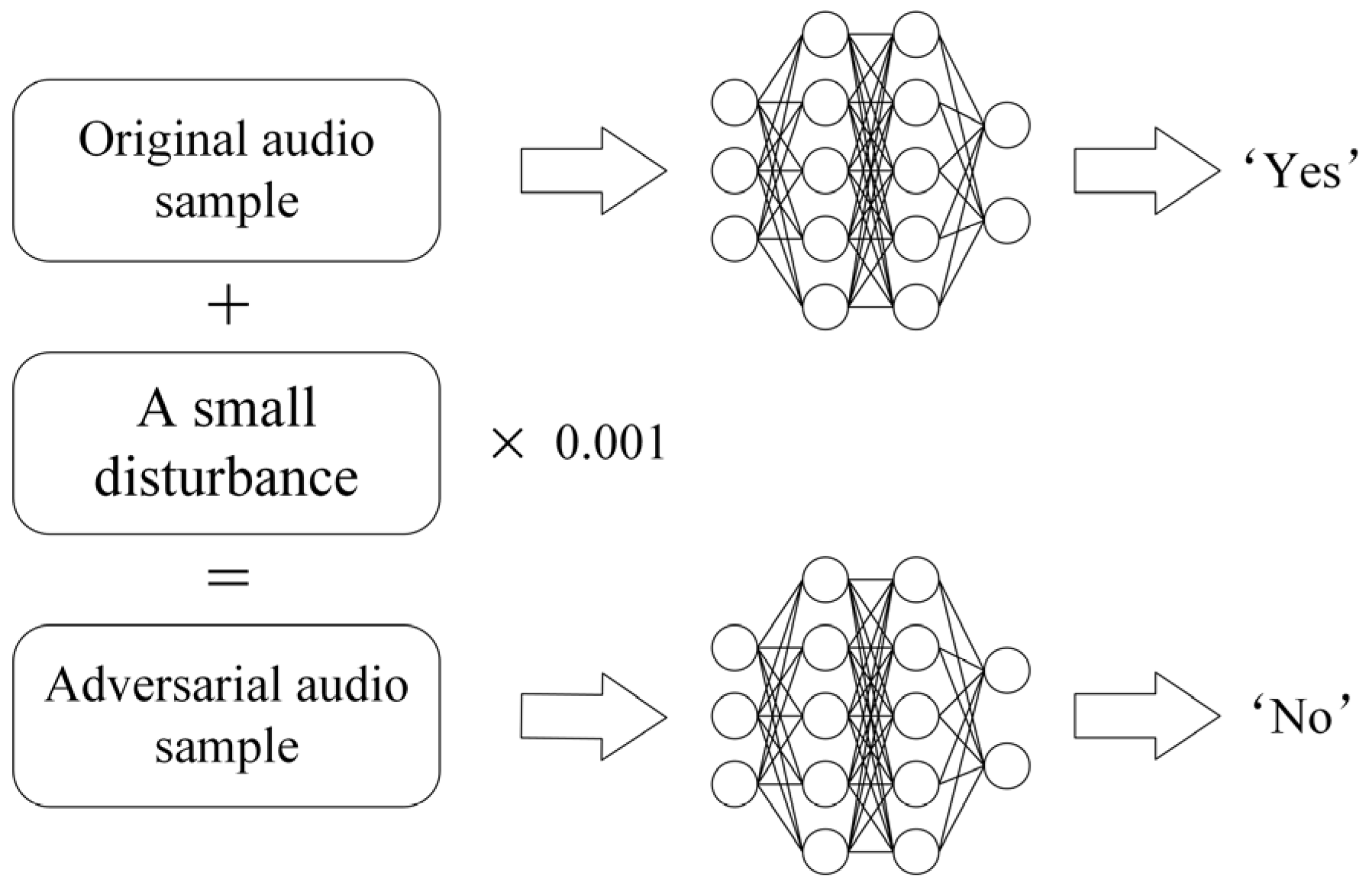
In 2018, Moustafa Alzantot demonstrated an adversarial attack on a speech classification model [12]. Figure 1 depicts the principle behind speech adversarial samples: an attacker introduces imperceptible noise to the speech, preserving its acoustic characteristics as perceived by the human ear while causing the speech recognition model to classify it as a different type of speech. These manipulated audio samples represent speech adversarial samples.
This study introduces a novel approach for the detection of speech adversarial samples, thereby enabling neural networks to defend against adversarial attacks based on black-box models. By conducting adversarial detection prior to the admission of speech data into the recognition model, identified speech adversarial samples are withheld from recognition, rather than being misclassified.
2. Related Work
In recent years, there have been numerous advancements in speech recognition technologies that are built upon deep learning models. Graves [13] employed connectionist temporal classification (CTC) to develop a state-of-the-art end-to-end speech recognition model that directly maps input acoustic feature sequences to output word sequences. Building upon this work, Baidu successfully commercialized speech recognition models for both English and Chinese languages through extensive data training [14]. Kubanek et al. proposed a novel approach that utilizes three independent convolutional layers: traditional temporal convolution and two different frequency convolutions. This technique enables the creation of sound patterns in the form of RGB images and proposes a method for segmenting continuous speech into syllables [15].
The generation of speech adversarial samples primarily involves two methods: gradient-based methods and black-box optimization-based methods [16,17]. Current research on adversarial samples is rooted in the study of neural network robustness. This research began with the work of Biggio and Szegedy et al., who explored adversarial samples for deep neural networks. They utilized gradient descent and L-BFGS to implement optimization-based attack strategies, which resulted in the generation of adversarial image samples. This breakthrough paved the way for generating adversarial samples in the machine learning domain.
In 2014, Goodfellow et al. [18] discovered that the linear characteristics of neural networks render them vulnerable to adversarial perturbations. They proposed the fast gradient sign method (FGSM) as the first proposed approach to provide adversarial samples for adversarial training, effectively enhancing the network’s robustness. Building upon these findings, Alexey Kurakin [19] and others advanced the FGSM to the iterative gradient symbolic method (IGSM) through a more sophisticated iterative optimization strategy. Additionally, in 2017, Aleksander Madry et al. proposed the projected gradient descent (PGD) method [20], which generates adversarial samples by repeatedly applying gradient descent steps during training. As a result, the generated adversarial samples exhibited improved performance and convincingly deceived the neural network model.
To address the issue that the defense system might analyze the output class of nontarget adversarial examples to determine the original class, Hyun Kwon et al. [21] proposed a method for generating nontarget adversarial examples. In the field of speech, Dan Iter and colleagues utilized adversarial samples generated by the fast gradient sign method and the fooling gradient sign method [22] to successfully deceive the automatic speech recognition model Wavenet. Notably, the generated adversarial audio exhibited imperceptible differences to the human ear. Furthermore, they proposed a method to convert adversarial mel-scale frequency cepstral coefficient (MFCC) features back into audio. This demonstrates the effectiveness of the adversarial sample generation method in the field of image recognition within the domain of speech recognition as well.
Carlini and Wagner [23] further validated the existence of adversarial samples in the speech domain by applying a white-box iterative optimization-based attack algorithm to the end-to-end implementation of Mozilla’s DeepSpeech. This experiment provided evidence that adversarial samples within the speech field can be utilized for targeted attacks.
Adversarial training [24] is a technique to bolster the robustness of speech recognition models against adversarial disturbances, which is achieved by incorporating adversarial examples during the training process. However, in 2018, Dimitris et al. [25] found that while adversarial training increased model robustness, it concurrently reduced the model’s recognition accuracy.
Constructing an adversarial sample detector is a defensive method that screens for adversarial samples before they enter the recognition models. Samizade [17] employed a Convolutional Neural Network (CNN) to detect minute perturbations in speech adversarial samples, while Li et al. [26] introduced a detection network akin to a VGG network structure, utilizing convolutional operations to capture subtle discrepancies between adversarial and genuine samples. Nonetheless, both approaches are limited to defending against specifically targeted white-box attack models.
The study of learning the manifold where data points are located is an area of research that has attracted significant attention. Manifold learning refers to a technique of nonlinear dimensionality reduction that aims to comprehend the inherent structure of high-dimensional data and map it to a lower-dimensional space, thereby facilitating better visualization, understanding, and analysis of the data. The primary objective of manifold learning is to reduce the dimensionality of data while preserving the local characteristics inherent to the data. Consequently, it is often employed for dimensionality reduction and feature extraction of high-dimensional datasets.
In 2000, Roweis and Saul proposed the LLE method [27] for manifold learning, which reconstructs the local structure of data based on local linear relationships and maps it to a lower-dimensional space while preserving these relationships. Shortly thereafter, Tenenbaum et al. proposed the ISOMAP method [28], which maintains the geodesic distance between data points by constructing a graph based on nearest-neighbor relationships and utilizes the geometric structure of the graph for dimensionality reduction. In 2008, Laurens van der Maaten and others suggested the t-distributed stochastic neighbor embedding (t-SNE) method [29], which constructs a probability distribution on pairs of high-dimensional data points in a manner that assigns a higher probability to similar objects. This method is often employed to preserve the similarity between data points in high-dimensional space while mapping the data to a lower-dimensional space, particularly for visualizing high-dimensional datasets.
In 2020, Leland McInnes proposed uniform manifold approximation and projection (UMAP), the most advanced manifold learning method [30]. UMAP is a practical and scalable algorithm that builds upon the theoretical foundations of Riemannian geometry and algebraic topology. It is capable of processing real-world data. In terms of visualization quality, the UMAP algorithm is a strong competitor to t-SNE and can preserve more global structures. Additionally, UMAP does not impose any computational restrictions on embedding dimensions, making it a versatile dimensionality reduction technique for machine learning applications.
Figure 2 illustrates the visual results of dimensionality reduction using manifold learning methods on the MNIST dataset. Tanay et al. [31] discovered that various types of data exhibit remarkable similarity in high-dimensional space, yet neural networks are capable of correctly classifying them. They proposed a boundary-tilted view, suggesting that adversarial samples tend to reside in close proximity to the classification boundary of the training data manifold. With regard to the manifold hypothesis of adversarial examples [32,33], it is assumed that adversarial examples deviate from the low-dimensional data manifold.
3. Audio Adversarial Sample Detection Method Based on Manifold Learning
Recent research has demonstrated that adversarial examples are located near the classification boundary of the training data manifold or deviate from the manifold. Building on this finding, this study proposes a speech adversarial sample detection method based on manifold learning.
In this section, we first discuss the manifold dimensionality reduction technique employed in this article. We will then introduce the adversarial sample detection method that relies on the results obtained from manifold learning dimensionality reduction. Finally, we present a speech adversarial sample detection method grounded in manifold learning.
3.1. Low-Dimensional Manifold Embedding of Speech Data
We utilize two leading manifold learning techniques, namely, t-SNE(t-distributed Stochastic Neighbor Embedding) and UMAP(t-distributed Stochastic Neighbor Embedding), to perform low-dimensional embedding on the speech dataset and compare the results.
3.1.1. t-SNE
t-SNE adopts a probability-based approach to measure the similarity between high-dimensional data points to preserve these similarities in low-dimensional space. By employing a specific probability distribution (t-distribution), t-SNE effectively handles outliers in high-dimensional data and generates improved clustering effects in low-dimensional space.
The calculation of similarity between data points in high-dimensional space involves computing a probability distribution for each data point, which determines its similarity to other data points. This distribution can be interpreted as a “neighbor relationship”.
Similarly, to determine a new position for each data point in the low-dimensional space and calculate the similarity between data points in this reduced space, t-distributed stochastic neighbor embedding (t-SNE) computes a probability distribution for each data point in the low-dimensional domain.
t-SNE leverages the Kullback–Leibler divergence (KL divergence) optimization technique to minimize the disparity between probability distributions in high- and low-dimensional spaces. By employing algorithms such as gradient descent, t-SNE aims to minimize this disparity and ensure that the distribution of data points in the low-dimensional space preserves as many of the similar relationships present in the high-dimensional space as possible.
The “t-distribution” used in t-SNE is a specific probability distribution function that effectively retains the local structure in low-dimensional space while placing more emphasis on distant data points. This approach greatly enhances the representation of the data structure in the reduced space.
3.1.2. UMAP
UMAP finds the nearest neighbors of a data point by using the nearest neighbor descent algorithm to identify the nearest neighbors of a given data point. Subsequently, UMAP constructs a graph by connecting these nearest neighbors. UMAP operates under the assumption that data points are uniformly distributed on the manifold, causing the spacing between points to stretch or compress based on local density. Consequently, the distance metric across space is not uniform but instead varies across regions. To control the dimensionality reduction process, UMAP employs the n_neighbors hyperparameter, which specifies the number of neighbors to consider.
During graph construction, it is essential to avoid numerous disconnected points that may hinder the learning of the desired manifold structure. To address this concern, UMAP utilizes the local_connectivity parameter (default value of 1). By setting local_connectivity to 1, each data point in the high-dimensional space is associated with another. The strength of the connections between the data points in the graph is represented by edge weights (w). Due to UMAP’s adoption of a different distance method, there may be discrepancies in edge weights from the perspective of individual points. For instance, the edge weights from points A to B may differ from the weights in the opposite direction. UMAP successfully resolves this issue by taking the union of both edges, resulting in a connected neighborhood graph.
UMAP calculates the distance between data points on the manifold using the standard Euclidean distance relative to the global coordinate system. The conversion from variable distance to standard distance also influences the distance between a data point and its nearest neighbor. Consequently, UMAP introduces a hyperparameter called min_dist (with a default value of 0.1) to define the minimum distance between the embedded points.
Upon specifying the minimum distance, UMAP proceeds to identify a superior low-dimensional representation of the manifold by minimizing the following cost function, also known as cross-entropy (CE):
where represents the edge connecting each pair of nearest neighbors, represents the known edge weight from the high-dimensional manifold approximation, and represents the edge weight to be discovered for the low-dimensional representation.
Whenever the weight associated with the high-dimensional case is larger, the first term () acts as the “attraction”. This is because this term will be minimized when is as large as possible, which occurs when the distance between points is as small as possible.
When the high-dimensional weight is small, the second term acts as a “repulsive force”. This is because by making as small as possible, the term will be minimized.
Ultimately, the interplay between these two “forces” brings the low-dimensional representation closer to an accurate representation of the overall topology of the original data.
The optimal weights of edges in a low-dimensional representation are sought as the ultimate goal. These weights are obtained by minimizing the cross-entropy function mentioned earlier. Finally, UMAP calculates the coordinates of each data point in the designated low-dimensional space.
3.1.3. Contrast
While t-SNE is limited to embedding dimensions of two and three, UMAP can preserve both local and global structures without this restriction.
The speech dataset and the target sample are subjected to manifold learning-based dimensionality reduction to be projected onto a low-dimensional manifold. The sample to be detected is then embedded on this low-dimensional manifold. By examining the geometric relationship between the speech adversarial sample and the speech dataset on the manifold, it is possible to determine whether the sample to be detected is a speech adversarial sample.
3.2. Detection Method for Speech Adversarial Samples
There are a total of types of original audio data. After dimensionality reduction, the centroid of each type is calculated, and the point nearest to the centroid is selected as the center point of that type of data. The distance between the center points of each type of audio data is found. The first indicator is set to determine the geometric relationship between the sample to be detected and the original audio sample:
In the formula, is set to 0.9 for this experiment. The distance between the audio sample to be detected and the center point of each type of original audio data in the reduced low-dimensional space is calculated, and the minimum value is . Research suggests that adversarial samples are located near the training data manifold’s classification boundary or deviate from the manifold. Therefore, speech adversarial samples should be relatively far from the centroid of various types of original audio data. If , the sample to be detected is far from the centroid of various types of original audio data and is suspected to be a speech adversarial sample.
However, due to the unknown and irregular manifold structure of speech data, many normal audio samples are also situated far from the centroid of various types of original audio data. Therefore, another decision criterion is set: a maximum neighbor search range (the value is set to 0.5 in this experiment). First, the neighbors of all center points within this range are searched, and the minimum number of neighbors is selected.
Next, we search for other data points within the range of the sample to be detected if any of the following two conditions are met when is met:
- The number of data points within the search range is much smaller than .
- There are multiple categories of data points within the search range, with no single category accounting for more than 60% of the total.
Then, it can be inferred that the speech sample to be detected is an adversarial audio sample.
4. Experiment and Result Analysis
4.1. Selection of Experimental Datasets
The speech dataset utilized in this experiment is TensorFlow’s official Speech_Commands [34]. A pretrained classification model was used, thereby treating speech recognition as a classification task for speech data.
A total of 10,000 voice commands with five different labels were chosen as the original dataset. Each command consists of an English word (e.g., go, stop). Each command is represented by more than 1700 voice files recorded by different speakers.
4.2. Selection of Speech Adversarial Samples
From a security standpoint, the primary threat to neural networks is black-box attacks, wherein the attacker does not need to comprehend the internal structure of the target network and can conduct model attacks merely by interacting with the target network.
This article employs the method proposed by Moustafa Alzantot et al., to generate speech adversarial samples. It randomly selects original audio samples for attack and generates 100 speech adversarial samples for subsequent experimental testing. This technique constitutes a black-box attack method that employs a gradient-free approach based on genetic algorithms to generate speech adversarial samples. The method relies solely on access to the input and output of the victim’s speech recognition system.
The speech adversarial samples generated using this technique enable listeners to perceive the sounds received as the original labels without the human ear’s final judgment being influenced by any noise, while the machine learning model misclassifies all of them.
4.3. MFCC Feature Extraction
Typically, automatic speech recognition (ASR) models employ MFCC features from the original audio as input. Consequently, the experiment in this article extracts MFCC features from the original speech data and speech adversarial samples. It then utilizes manifold learning techniques to capture the low-dimensional manifold and identify the geometric relationship between the original speech data and the speech adversarial samples.
In this experiment, the voice data are divided into 101 frames, and MFCC features are extracted from each frame. Each frame’s MFCC features comprise 13 coefficients. Therefore, the resulting MFCC feature data constitute a two-dimensional array with dimensions of 13 × 101. Figure 3 depicts the results of MFCC extraction according to the aforementioned criteria on a voice command labeled ‘go’ and a speech adversarial sample generated by perturbing the voice.
4.4. Low-Dimensional Embedding of Speech Data in Manifold Space and Detection of Speech Adversarial Samples
4.4.1. Results
After performing low-dimensional embedding on the speech dataset and the samples to be detected using t-SNE and UMAP, the method proposed in this article for detecting speech adversarial samples is applied to identify potential adversarial attacks.
In the experiments, it was observed that the t-SNE and UMAP manifold learning methods are sensitive to the number of nearest neighbor searches (n_neighbors) during the dimensionality reduction process. This study restricts the embedding dimension to three dimensions and conducts experiments by varying the number of nearest neighbor searches in the manifold learning method. The impact of these different parameter settings on the final detection results of the speech adversarial samples is observed. The impact of adjusting the number of nearest neighbor searches for t-SNE and UMAP respectively on the detection success rate is shown in Table 1 and Table 2. Subsequently, the optimal number of nearest neighbor searches is determined for both t-SNE and UMAP under specific speech datasets and adversarial sample detection tasks to achieve better results in speech adversarial sample detection.
Experimental results demonstrate that compared with t-SNE, the low-dimensional data manifold obtained through dimensionality reduction in the speech dataset using UMAP exhibits superior performance in detecting speech adversarial samples.
As manifold learning technologies, t-SNE and UMAP demonstrate excellent visualization capabilities. t-SNE is adept at capturing local structures and clustering patterns, while UMAP is better equipped to preserve the global data structure and handle large-scale and high-dimensional data. During the experiment, the embedding conditions were set to two-dimensional and three-dimensional to better visualize the results of t-SNE and UMAP when appropriate parameters were applied. Through the visualization of these experimental results, the internal structure of speech data can be more comprehensively understood and presented. Additionally, the characteristics, patterns, and geometric relationships between speech adversarial samples and original speech samples can be analyzed at a low-dimensional level.
4.4.2. Visualization
As depicted in Figure 4, the speech data exhibit evident clustering effects and distinct boundaries between different data types following dimensionality reduction. However, due to the constraints of low dimensions, the visualization results are severely limited in terms of the information they can convey.
The process of mapping high-dimensional data to a low-dimensional space in dimensionality reduction inherently involves information loss. While the visualization results present clustering effects and clear boundaries, the information represented in lower dimensions only offers a partial projection of the original data and may fail to fully depict the complex structure and detailed characteristics of the data.
Furthermore, excessively low dimensionality constraints can give rise to issues such as information compression and data overlap, impeding the clear expression of the true relationship between subsets of data points.
According to the 2D visualization results shown in Figure 4, although similar data points cluster effectively, the substantial loss of features leads to the overlap of different data types, preventing an accurate representation of the geometric relationships within the speech data. By increasing the embedding dimension to three, the visualization results of the speech dataset are presented in Figure 5. This increase in dimensionality allows for the representation of additional data points, revealing numerous hidden data points that remain concealed when limited to two dimensions. All five types of data selected for the experiment are exhibited in the visualization results. The geometric relationships among speech data may be portrayed more clearly in a three-dimensional space. And the visualization results show conclusions that align with the experimental results. Irrespective of whether the embedding dimension is limited to two or three dimensions, the clustering efficacy of UMAP in reducing the dimensionality of the speech dataset significantly surpasses that of t-SNE.
Compared to two dimensions, a three-dimensional space retains a relatively larger number of speech data features, captures the complexity and diversity of the data more effectively, and provides a wider range of perspectives and a more comprehensive observation space.
While t-SNE restricts the embedding dimensions to two and three, UMAP imposes no such limitations. Therefore, the advantages of manifold learning technology at the visualization level can be discarded in favor of further enhancing the embedding dimension. Even so, the dimension of the MFCC feature of the speech data is reduced from 13 × 101 to single digits, resulting in a significant reduction in the computational cost of subsequent processes.
By increasing the dimension of manifold embedding, the success rate of detecting speech adversarial samples can be improved to some extent, and in some cases, even better results can be achieved. Under different manifold learning embedding dimensions, the changes in detection success rate are shown in Table 3. Enhanced by UMAP, the detection success rate for speech adversarial samples reached 84.73%, significantly surpassing the performance of t-SNE. However, it is important to note that while increasing the embedding dimension may lead to better detection results, having a dimension that is too high can result in unnecessary problems, particularly when one of the advantages of manifold learning technology is its ability to significantly reduce computational costs.
The detection methods for speech adversarial samples proposed by Samizade et al. [17] and Li et al. [26] have achieved a success rate of over 99% in identifying adversarial samples crafted by specified white-box models. However, their defensive efficacy significantly declines when attackers switch their methods, and these methods fail to detect adversarial samples produced by black-box models. This study puts forward a manifold learning-based detection method for speech adversarial samples, boasting a success rate of 84.73%, capable of detecting samples generated by black-box models and exhibiting a certain degree of transferability.
5. Conclusions
This study proposes a novel method for detecting speech adversarial samples by analyzing the geometric relationship between the sample to be detected and the original audio sample on a low-dimensional manifold. The experiment focuses on speech adversarial samples generated through black-box attack methods, as these adversaries do not require an understanding of the internal structure of the target network and can achieve model attacks simply by inputting speech adversarial samples into the target network. Furthermore, the commonly used method of training neural networks with adversarial samples to improve model robustness is not effective against adversarial samples generated through black-box attack methods.
Through the use of manifold learning, important features can be extracted, and data representation can be simplified, leading to a significant reduction in data dimensionality and the amount of computation required for the processing, storage, and analysis of data. This advantage allows manifold learning to train models more efficiently when dealing with large-scale datasets or high-dimensional data.
Additionally, this paper demonstrates through experiments that manifold learning can provide intuitive and easily understandable visualization results for high-dimensional speech data. By visualizing high-dimensional speech features in a more comprehensible space, the inherent structure and characteristics of speech data can be observed more clearly.
Recent research has shown that training neural networks using adversarial examples can effectively enhance model robustness. However, this approach also reduces model accuracy due to the incorporation of adversarial examples as inputs. The method proposed in this article allows for the detection of speech data adversarial examples prior to their input into the machine learning model, thus avoiding the negative impact of training on adversarial samples.
Author Contributions
Writing—original draft preparation, X.M.; writing—review and editing, D.X.; visualization, C.Y.; project administration, P.L.; supervision, D.L. All authors have read and agreed to the published version of the manuscript.
Funding
This work was funded by the Shandong Provincial Natural Science Foundation (No. ZR2019PF007), basic scientific research operating expenses of Shandong University (No. 2018ZQXM004), the National Natural Science Foundation of China (No. 62076149 and No. 62376136), the Young Scholars Program of Shandong University, Weihai (No. 1050501318006), and the Science and Technology Development Plan of Weihai City (No. 1050413421912).
Data Availability Statement
Data are contained within the article.
Conflicts of Interest
The authors declare no conflicts of interest.
References
- Hu, Q.; Lu, Y.; Pan, Z.; Gong, Y.; Yang, Z. Can AI artifacts influence human cognition? The effects of artificial autonomy in intelligent personal assistants. Int. J. Inf. Manag. 2021, 56, 102250. [Google Scholar] [CrossRef]
- Wang, D.; Wang, X.; Lv, S. An Overview of End-to-End Automatic Speech Recognition. Symmetry 2019, 11, 1018. [Google Scholar] [CrossRef]
- Szegedy, C.; Zaremba, W.; Sutskever, I.; Bruna, J.; Erhan, D.; Goodfellow, I.; Fergus, R. Intriguing properties of neural networks. arXiv 2013, arXiv:1312.6199. [Google Scholar] [CrossRef]
- Papernot, N.; McDaniel, P.; Jha, S.; Fredrikson, M.; Berkay Celik, Z.; Swami, A. The Limitations of Deep Learning in Adversarial Settings. arXiv 2015, arXiv:1511.07528. [Google Scholar] [CrossRef]
- Pedraza, A.; Deniz, O.; Bueno, G. On the Relationship between Generalization and Robustness to Adversarial Examples. Symmetry 2021, 13, 817. [Google Scholar] [CrossRef]
- Petracca, G.; Sun, Y.; Jaeger, T.; Atamli, A. AuDroid. In Proceedings of the 31st Annual Computer Security Applications Conference, Los Angeles, CA, USA, 7–11 December 2015; pp. 181–190. [Google Scholar]
- Edu, J.S.; Such, J.M.; Suarez-Tangil, G. Smart Home Personal Assistants: A Security and Privacy Review. arXiv 2019, arXiv:1903.05593. [Google Scholar] [CrossRef]
- Kabir, M.M.; Mridha, M.F.; Shin, J.; Jahan, I.; Ohi, A.Q. A Survey of Speaker Recognition: Fundamental Theories, Recognition Methods and Opportunities. IEEE Access 2021, 9, 79236–79263. [Google Scholar] [CrossRef]
- Kurzekar, P.K.; Deshmukh, R.R.; Waghmare, V.B.; Shrishrimal, P.P. A Comparative Study of Feature Extraction Techniques for Speech Recognition System. Int. J. Innov. Res. Sci. Eng. Technol. 2014, 3, 18006–18016. [Google Scholar] [CrossRef]
- Du, T.; Ji, S.; Li, J.; Gu, Q.; Wang, T.; Beyah, R. SirenAttack: Generating Adversarial Audio for End-to-End Acoustic Systems. In Proceedings of the 15th ACM Asia Conference on Computer and Communications Security, Taipei, Taiwan, 5–9 October 2020; pp. 357–369. [Google Scholar]
- Chowdhury, A.; Ross, A. Fusing MFCC and LPC Features Using 1D Triplet CNN for Speaker Recognition in Severely Degraded Audio Signals. IEEE Trans. Inf. Forensics Secur. 2020, 15, 1616–1629. [Google Scholar] [CrossRef]
- Alzantot, M.; Balaji, B.; Srivastava, M. Did you hear that? Adversarial Examples Against Automatic Speech Recognition. arXiv 2018, arXiv:1801.00554. [Google Scholar] [CrossRef]
- Graves, A.; Mohamed, A.-R.; Hinton, G. Speech Recognition with Deep Recurrent Neural Networks. arXiv 2013, arXiv:1303.5778. [Google Scholar] [CrossRef]
- Hannun, A.; Case, C.; Casper, J.; Catanzaro, B.; Diamos, G.; Elsen, E.; Prenger, R.; Satheesh, S.; Sengupta, S.; Coates, A.; et al. Deep Speech: Scaling up end-to-end speech recognition. arXiv 2014, arXiv:1412.5567. [Google Scholar] [CrossRef]
- Kubanek, M.; Bobulski, J.; Kulawik, J. A Method of Speech Coding for Speech Recognition Using a Convolutional Neural Network. Symmetry 2019, 11, 1185. [Google Scholar] [CrossRef]
- Chen, P.-Y.; Zhang, H.; Sharma, Y.; Yi, J.; Hsieh, C.-J. Zoo. In Proceedings of the 10th ACM Workshop on Artificial Intelligence and Security, Dallas, TX, USA, 3 November 2017; pp. 15–26. [Google Scholar]
- Samizade, S.; Tan, Z.-H.; Shen, C.; Guan, X. Adversarial Example Detection by Classification for Deep Speech Recognition. arXiv 2019, arXiv:1910.10013. [Google Scholar] [CrossRef]
- Goodfellow, I.J.; Shlens, J.; Szegedy, C. Explaining and Harnessing Adversarial Examples. arXiv 2014, arXiv:1412.6572. [Google Scholar] [CrossRef]
- Kurakin, A.; Goodfellow, I.; Bengio, S. Adversarial examples in the physical world. arXiv 2016, arXiv:1607.02533. [Google Scholar] [CrossRef]
- Madry, A.; Makelov, A.; Schmidt, L.; Tsipras, D.; Vladu, A. Towards Deep Learning Models Resistant to Adversarial Attacks. arXiv 2017, arXiv:1706.06083. [Google Scholar] [CrossRef]
- Kwon, H.; Kim, Y.; Yoon, H.; Choi, D. Random Untargeted Adversarial Example on Deep Neural Network. Symmetry 2018, 10, 738. [Google Scholar] [CrossRef]
- Iter, D.; Huang, J.; Jermann, M. Generating Adversarial Examples for Speech Recognition. 2017. Available online: https://www.semanticscholar.org/paper/Generating-Adversarial-Examples-for-Speech-Iter-Huang/9181ac1edb3ef0e56447e9da66de2cbd7f8dcff6 (accessed on 8 April 2024).
- Carlini, N.; Wagner, D. Audio Adversarial Examples: Targeted Attacks on Speech-to-Text. In Proceedings of the 2018 IEEE Security and Privacy Workshops (SPW), San Francisco, CA, USA, 24 May 2018; pp. 1–7. [Google Scholar]
- Sun, S.; Guo, P.; Xie, L.; Hwang, M.-Y. Adversarial Regularization for Attention Based End-to-End Robust Speech Recognition. IEEE/ACM Trans. Audio Speech Lang. Process. 2019, 27, 1826–1838. [Google Scholar] [CrossRef]
- Tsipras, D.; Santurkar, S.; Engstrom, L.; Turner, A.; Madry, A. Robustness May Be at Odds with Accuracy. arXiv 2018, arXiv:1805.12152. [Google Scholar] [CrossRef]
- Li, X.; Li, N.; Zhong, J.; Wu, X.; Liu, X.; Su, D.; Yu, D.; Meng, H. Investigating Robustness of Adversarial Samples Detection for Automatic Speaker Verification. arXiv 2020, arXiv:2006.06186. [Google Scholar] [CrossRef]
- Roweis, S.T.; Saul, L.K. Nonlinear Dimensionality Reduction by Locally Linear Embedding. Science 2000, 290, 2323–2326. [Google Scholar] [CrossRef] [PubMed]
- Tenenbaum, J.B.; Silva, V.d.; Langford, J.C. A Global Geometric Framework for Nonlinear Dimensionality Reduction. Science 2000, 290, 2319–2323. [Google Scholar] [CrossRef] [PubMed]
- Van der Maaten, L.; Hinton, G. Visualizing data using t-SNE. J. Mach. Learn. Res. 2008, 9, 2579–2605. [Google Scholar]
- McInnes, L.; Healy, J.; Melville, J. UMAP: Uniform Manifold Approximation and Projection for Dimension Reduction. arXiv 2018, arXiv:1802.03426. [Google Scholar] [CrossRef]
- Tanay, T.; Griffin, L. A Boundary Tilting Persepective on the Phenomenon of Adversarial Examples. arXiv 2016, arXiv:1608.07690. [Google Scholar] [CrossRef]
- Gilmer, J.; Metz, L.; Faghri, F.; Schoenholz, S.S.; Raghu, M.; Wattenberg, M.; Goodfellow, I. Adversarial Spheres. arXiv 2018, arXiv:1801.02774. [Google Scholar] [CrossRef]
- Glorot, X.; Bengio, Y. Understanding the difficulty of training deep feedforward neural networks. In Proceedings of the Thirteenth International Conference on Artificial Intelligence and Statistics, Sardinia, Italy, 13–15 May 2010; pp. 249–256. [Google Scholar]
- Warden, P. Speech Commands: A Dataset for Limited-Vocabulary Speech Recognition. arXiv 2018, arXiv:1804.03209. [Google Scholar] [CrossRef]
Figure 1.
The principle of speech adversarial samples: by adding a small disturbance, the neural network will misrecognize the input speech.
Figure 1.
The principle of speech adversarial samples: by adding a small disturbance, the neural network will misrecognize the input speech.

Figure 2.
Visualization results of dimensionality reduction on the MNIST dataset using LLE, ISOMAP, t-SNE, and UMAP.
Figure 2.
Visualization results of dimensionality reduction on the MNIST dataset using LLE, ISOMAP, t-SNE, and UMAP.

Figure 3.
(a) MFCC feature extraction diagram of the voice command labeled ‘go’; (b) MFCC feature extraction diagram of the speech adversarial sample generated by interfering with the voice command labeled ‘go’.
Figure 3.
(a) MFCC feature extraction diagram of the voice command labeled ‘go’; (b) MFCC feature extraction diagram of the speech adversarial sample generated by interfering with the voice command labeled ‘go’.

Figure 4.
Visualization results after using t-SNE (a) and UMAP (b) to reduce the speech dataset and the samples to be detected to 2 dimensions.
Figure 4.
Visualization results after using t-SNE (a) and UMAP (b) to reduce the speech dataset and the samples to be detected to 2 dimensions.

Figure 5.
Visualization results after using t-SNE (a) and UMAP (b) to reduce the speech dataset and the samples to be detected to 3 dimensions.
Figure 5.
Visualization results after using t-SNE (a) and UMAP (b) to reduce the speech dataset and the samples to be detected to 3 dimensions.


Table 1.
Detection success rate based on t-SNE under different numbers of nearest neighbor searches when the embedding dimension is limited to 3 dimensions.
Table 1.
Detection success rate based on t-SNE under different numbers of nearest neighbor searches when the embedding dimension is limited to 3 dimensions.
| Algorithm | n_Neighbors | Detection Success Rate |
|---|---|---|
| t-SNE | 15 | 36.74% |
| 20 | 48.05% | |
| 25 | 53.96% | |
| 30 | 55.32% | |
| 35 | 43.37% |
Table 2.
Detection success rate based on UMAP under different numbers of nearest neighbor searches when the embedding dimension is limited to 3 dimensions.
Table 2.
Detection success rate based on UMAP under different numbers of nearest neighbor searches when the embedding dimension is limited to 3 dimensions.
| Algorithm | n_Neighbors | Detection Success Rate |
|---|---|---|
| UMAP | 5 | 34.26% |
| 10 | 59.75% | |
| 11 | 73.47% | |
| 12 | 66.46% | |
| 15 | 57.32% |
Table 3.
Adversarial sample detection results after low-dimensional manifold embedding restricted to different dimensions using t-SNE and UMAP.
Table 3.
Adversarial sample detection results after low-dimensional manifold embedding restricted to different dimensions using t-SNE and UMAP.
| Algorithm | Embed Dimension Restrictions | Detection Success Rate |
|---|---|---|
| t-SNE | 2 | 36.28% |
| 3 | 55.32% | |
| UMAP | 2 | 44.56% |
| 3 | 73.47% | |
| 4 | 84.73% | |
| 5 | 80.24% |
Disclaimer/Publisher’s Note: The statements, opinions and data contained in all publications are solely those of the individual author(s) and contributor(s) and not of MDPI and/or the editor(s). MDPI and/or the editor(s) disclaim responsibility for any injury to people or property resulting from any ideas, methods, instructions or products referred to in the content. |
© 2024 by the authors. Licensee MDPI, Basel, Switzerland. This article is an open access article distributed under the terms and conditions of the Creative Commons Attribution (CC BY) license (https://creativecommons.org/licenses/by/4.0/).
Share and Cite
MDPI and ACS Style
Ma, X.; Xu, D.; Yang, C.; Li, P.; Li, D. A Speech Adversarial Sample Detection Method Based on Manifold Learning. Mathematics 2024, 12, 1226. https://doi.org/10.3390/math12081226
AMA Style
Ma X, Xu D, Yang C, Li P, Li D. A Speech Adversarial Sample Detection Method Based on Manifold Learning. Mathematics. 2024; 12(8):1226. https://doi.org/10.3390/math12081226
Chicago/Turabian StyleMa, Xiao, Dongliang Xu, Chenglin Yang, Panpan Li, and Dong Li. 2024. "A Speech Adversarial Sample Detection Method Based on Manifold Learning" Mathematics 12, no. 8: 1226. https://doi.org/10.3390/math12081226
Note that from the first issue of 2016, this journal uses article numbers instead of page numbers. See further details here.