Inter-Channel Correlation Modeling and Improved Skewed Histogram Shifting for Reversible Data Hiding in Color Images

Abstract

Reversible data hiding (RDH) is an advanced data protection technology that allows the embedding of additional information into an original digital medium while maintaining its integrity. Color images are typical carriers for information because of their rich data content, making them suitable for data embedding. Compared to grayscale images, color images with their three color channels (RGB) enhance data embedding capabilities while increasing algorithmic complexity. When implementing RDH in color images, researchers often exploit the inter-channel correlation to enhance embedding efficiency and minimize the impact on image visual quality. This paper proposes a novel RDH method for color images based on inter-channel correlation modeling and improved skewed histogram shifting. Initially, we construct an inter-channel correlation model based on the relationship among the RGB channels. Subsequently, an extended method for calculating the local complexity of pixels is proposed. Then, we adaptively select the pixel prediction context and design three types of extreme predictors. The improved skewed histogram shifting method is utilized for data embedding and extraction. Finally, experiments conducted on the USC-SIPI and Kodak datasets validate the superiority of our proposed method in terms of image fidelity.

1. Introduction

Color images are an essential form of visual information communication and recording. The advent of the digital era has facilitated the generation, processing, transmission, and application of color images [1]. However, with the continuous development of information technology and the increasing complexity of the network environment, the security and privacy protection of color images face increasingly severe challenges. On the Internet, color images may risk being illegally obtained, tampered with, and disseminated, leading to severe consequences, such as personal privacy and commercial secret leakage [2,3]. Therefore, ensuring the security and privacy protection of color images is essential for protecting personal and commercial interests. In recent years, reversible data hiding (RDH) technology [4,5] has attracted wide attention as an effective means of information hiding. RDH technology can embed secret data into images while keeping the original image undamaged. RDH technology has higher security and concealment than traditional encryption techniques because it does not change the visual effect of the original image, making it challenging to discover and break. Therefore, using RDH technology to protect the security and privacy of color images has crucial theoretical value and practical significance. This paper proposes a novel RDH method for reversible data hiding and extraction in color images. Our goal is to enhance both the visual quality and privacy protection level of color images while ensuring the reversibility of data hiding, thereby providing an effective solution for the secure transmission and storage of color images.

RDH algorithms are primarily focused on grayscale images, with existing research mainly comprising four categories, namely, lossless compression [6], difference expansion (DE) [7,8,9], histogram shifting (HS) [10,11,12], and prediction error expansion (PEE) [13]. Lossless compression [6], the earliest RDH scheme, releases space by losslessly compressing some image features to embed secret data. However, this method suffers from limited embedding capacity. The DE method, pioneered by Tian [7], involves expanding the differences between adjacent pixels to embed secret data, with a maximum embedding rate of 0.5 bits per pixel (bpp). Subsequently, Ni et al. [10] proposed an HS-based method that builds the histogram of the original image and embeds data using peak and zero pixels. Methods based on DE and HS have undergone extensive research and improvement by numerous scholars. Qiu et al. [14] introduced an adaptive RDH method based on generalized integer transformation, while Wang et al. [15] presented a pixel distortion optimization method based on multiple histogram shifting. To improve the embedding performance of RDH schemes, Thodi and Rodriguez [13] proposed a PEE-based method that embeds data by expanding the differences between pixels and predicted values. PEE is an extension of the DE-based method and is considered the most effective and significant method. Subsequent methods have further improved pixel predictors based on PEE, including the median edge detection predictor [16], gradient adjusted predictor [17], rhombus predictor [18], and adaptive predictor [19,20]. In [21], the team explored and reviewed existing pixel predictors.

Color images are widely used in various application scenarios [1,22,23], while traditional RDH methods are mainly designed for grayscale images and are difficult to apply directly to color images. Thus, there is an urgent need to research and develop RDH techniques tailored for color images. Color images are much more complex and informative than grayscale images, involving multiple aspects of features such as inter-channel correlation, color information, and spatial structure. These features need to be finely processed and analyzed. In recent years, some scholars have started to focus on the research of RDH methods for color images and have achieved some preliminary results. This paper divides RDH methods for color images into three categories. The first category of methods utilizes the inter-channel correlation of color images for data embedding. Li et al. [24] employed a diamond predictor to predict the pixel values of each color channel and adjust the prediction values according to the edge information of another channel to improve the pixel prediction accuracy. Qi et al. [25] proposed a color image RDH method based on adaptive three-dimensional histogram modification that realizes data embedding and extraction by adjusting the three-dimensional histogram. Kong et al. [26] utilized the pixel difference value ordering between different color channels and proposed a color image RDH scheme based on multi-channel difference value ordering that could adaptively select the embedding channel, thereby improving the embedding capacity and image quality. The second category of methods is based on PEE for data embedding. Yao et al. [27] presented a color image RDH method based on guided filtering that utilizes guided filtering to enhance the effect of PEE. Mao et al. [28] proposed a color image RDH method based on channel unified embedding that realizes data hiding by performing unified data embedding operations on the channels. In addition, Mao et al. [29] utilized the pixel value ordering between color channels and proposed a color image RDH scheme based on the overall process channel correlation that could effectively utilize the image’s spatial structure and color information and improve the image quality. The third category of methods introduces a payload allocation strategy to optimize the data hiding performance. Ou et al. [30] proposed an efficient color image RDH method based on channel-related payload partitioning and adaptive embedding that performs payload partitioning according to the channel correlation and adapts an adaptive embedding strategy to optimize the data hiding effect. Kumar et al. [31] introduced a color image steganography scheme that leverages gray invariance within the AMBTC compression domain.

Despite some progress made in RDH research for color images, there are still limitations that need to be addressed. These shortcomings mainly manifest in the following three aspects:

• Some methods are merely extensions of RDH techniques for grayscale images, failing to fully exploit the characteristics of color images and the correlation between channels, thus limiting their data embedding capacity.
• In pursuit of increasing embedding capacity, specific methods may compromise image quality as they fail to effectively balance the relationship between embedding capacity and image quality, resulting in pixel distortion introduced by the data embedding algorithm.
• Efficiency is compromised in some methods when dealing with large-capacity data because of their high algorithm complexity, leading to increased computational costs and a lack of practical parallel computing or other efficient techniques, thereby reducing their efficiency in processing large-capacity data.

After analyzing the limitations of existing RDH methods for color images, seeking practical solutions and innovative approaches becomes crucial. Accordingly, this paper proposes a novel RDH technique tailored for color images that can overcome the existing limitations and contribute to the development of RDH in color images. This paper proposes an RDH method for color images that leverages inter-channel correlation to calculate pixel complexity and enhances the skewed histogram shifting technique for efficient data embedding and extraction. We endeavor to enhance the security and privacy protection levels of color images and provide an effective solution for the secure transmission and storage of color images. The innovative and contributory aspects of this paper can be outlined as follows:

• A novel inter-channel correlation modeling method is proposed. A referential relationship between channels is established through the calculation of the correlation among the R, G, and B channels of color images. By accurately modeling the inter-channel correlations, an enhanced evaluation of pixel local complexity is achievable, mitigating the pixel distortion induced by data embedding.
• An extended method for calculating the local complexity of pixels is proposed. This method leverages the inter-channel correlation model to expand upon the general local complexity calculation approach. The extended method captures images’ local texture features and structural information more accurately, thereby guiding the data embedding process better.
• An improved skewed histogram shifting method is proposed. Based on the inter-channel correlation model, the pixel prediction context is adaptively selected, and a generation method for pairs of extreme predictors is proposed to refine skewed histogram shifting. This method enhances the accuracy and reliability of data embedding and reduces distortion during the embedding process.

The structure of this paper is organized as follows. Section 2 provides a review of existing works related to RDH. Section 3 elaborates on the proposed method of inter-channel correlation modeling and the improved skewed histogram shifting algorithm. Section 4 validates the effectiveness of the proposed method through a series of experiments and analyzes the experimental results. Finally, Section 5 concludes the research findings of this paper and suggests future research directions.

2. Related Work

This section provides a concise review of the related work. Section 2.1 revisits various methods for calculating local complexity, including the four-pixel, pairwise [32], and extended-pixel methods [33]. Subsequently, Section 2.2 discusses the skewed histogram shifting technique and the construction of extreme predictors as proposed in [33].

2.1. Methods for Calculating Local Complexity

Local complexity refers to the degree of intricacy or variation in the area surrounding a pixel within a digital image. Generally, higher local complexity indicates richer texture, structure, or color changes around the pixel, whereas lower local complexity suggests a relatively uniform or simple surrounding region. Evaluating local complexity allows for a deeper understanding of the image’s detailed features and facilitates tasks such as data hiding or processing in image processing applications. Selecting pixels with lower local complexity for data embedding is advantageous because these pixels typically possess fewer texture and structure features. Compared to pixels with higher complexity, they are more capable of concealing additional data without causing significant visual changes. This selection helps minimize distortion in the image after embedding while enhancing the stealthiness and stability of data embedding.

In Figure 1a, the current pixel is denoted as P, and its local complexity context includes the pixels in the four directions north, south, west, and east of P, labeled as N, S, W, and E, respectively. The local complexity of P is represented by $LC\left(P\right)$ and is calculated as follows:

$$LC\left(P\right)=\left|N-W\right|+\left|W-S\right|+\left|S-E\right|+\left|N-E\right|+\left|W-E\right|+\left|N-S\right|.$$

(1)

Ou et al. [32] improved the calculation method of $LC\left(P\right)$ by adopting a pairwise context, as shown in Figure 1b. The current pixel is denoted as $P_1$, and its local complexity context includes the eight surrounding pixels, namely, $N_1$, $S_1$, $W_1$, $E_1$, $F_1$, $F_2$, $E_2$, and $S_2$. In this case, the local complexity of $P_1$ is calculated by

$$\begin{array}{cc}\hfill L{C}_{pair}\left(P_1\right)=& \left|N_1-W_1\right|+\left|W_1-S_1\right|+\left|S_1-E_1\right|+\left|N_1-E_1\right|+\left|S_1-S_2\right|\hfill \\ \hfill & +\left|S_2-E_2\right|+\left|E_2-E_1\right|+\left|E_1-F_2\right|+\left|S_2-F_2\right|.\hfill \end{array}$$

(2)

Kim et al. [33] enhanced the calculation method of $L{C}_{pair}\left(P_1\right)$ by adopting an extended context, as illustrated in Figure 1c. The current pixel remains P, and its local complexity context includes more pixels than in Figure 1a,b. The calculation of local complexity in Figure 1c is extended to include the local complexities of the $NW$, $NE$, $SW$, and $SE$ pixels. Therefore, the calculation formula for $L{C}_e\left(P\right)$ is

$$L{C}_e\left(P\right)=LC\left(P\right)+LC\left(NW\right)+LC\left(NE\right)+LC\left(SE\right)+LC\left(SW\right).$$

(3)

2.2. Skewed Histogram Shifting

Traditional HS-based methods utilize the Laplacian distribution characteristics of the prediction error histogram for histogram shifting. HS embeds data in the most frequently occurring errors to increase embedding capacity while minimizing distortion. Kim et al. [33] proposed skewed histogram shifting as an enhancement to traditional HS. Symmetric histogram is illustrated in Figure 2a, while left-skewed and right-skewed histograms are depicted in Figure 2b,c, respectively. In contrast to symmetric histograms, skewed histograms exhibit long and short tails. Data embedding based on skewed histograms involves three main steps: generating a pair of extreme predictions for the current pixel, embedding data using positive histogram shifting (PHS), and embedding data using negative histogram shifting (PHS). Positive histograms are generated from prediction errors where the difference between the pixel and predicted values is positive. In contrast, negative histograms are generated from prediction errors with negative differences.

The generation of extreme predictions is crucial in skewed histogram shifting, and a pair of extreme predictors is represented as $(H_h,H_l)$. For the current pixel P, $H_h$, and $H_l$ are generated using the pixels in the north, south, west, and east directions, denoted as N, S, W, and E, respectively (as shown in Figure 1a). First, N, S, W, and E are sorted in ascending order, represented as ${\delta }_1$, ${\delta }_2$, ${\delta }_3$, and ${\delta }_4$, respectively, with ${\delta }_1\le {\delta }_2\le {\delta }_3\le {\delta }_4$. Three predictors are used to generate $H_h$ and $H_l$, and the details of predictors 1, 2, and 3 are shown in

Table 1. Three predictors used to generate extreme predictors.

Predictor Number	1	2	3
$H_h$	${\delta }_4$	$\left[\frac{{\delta }_4+{\delta }_3}{2}\right]$	$\left[\frac{{\delta }_4+{\delta }_3+{\delta }_2}{3}\right]$
$H_l$	${\delta }_1$	$\left[\frac{{\delta }_4+{\delta }_3}{2}\right]$	$\left[\frac{{\delta }_3+{\delta }_2+{\delta }_1}{3}\right]$

. In Table 1, $[.]$ denotes rounding to the nearest integer value. Predictor 1 generates $H_h$ and $H_l$ using the maximum and minimum values, respectively, while predictor 2 calculates the average of the two maximum and two minimum values. Predictor 3 utilizes the average of the three maximum and three minimum values. Additionally, to avoid duplicate embedding when $H_h$ and $H_l$ are equal, special treatment is applied to $H_l$ to ensure the uniqueness and accuracy of the embedding. The processing of $H_l$ is as follows:

$$H_l=\left\{\begin{array}{cc}{H}_l-1,\hfill & \mathrm{if}{H}_h=H_l\hfill \\ H_l,\hfill & \mathrm{otherwise}\hfill \end{array}\right..$$

(4)

3. Methodology

In this section, we provide a comprehensive exposition of the proposed method, encompassing the modeling of inter-channel pixel correlation, the computation of pixel local complexity, the generation of a pair of extreme predictors in skewed histogram shifting, the details of data embedding and extraction, as well as the overall algorithm implementation process.

3.1. Inter-Channel Correlation Modeling

In contrast to grayscale images, which are made up of a single channel, color images are composed of three distinct channels: R, G, and B. Color images offer a broader space for data embedding. Grasping the interplay between color channels enhances the comprehension of an image’s intricate structure and the richness of its content. Analyzing the interactions between channels makes it possible to more accurately capture the changing characteristics of pixel values and texture information in images, thereby enhancing the accuracy and richness of image representation. Particularly in RDH algorithms, leveraging the correlation between channels can enhance the accuracy of pixel local complexity calculation and pixel prediction, thereby achieving more efficient data embedding and extraction performance.

When analyzing the pixel characteristics and texture structure of the RGB channels, we observed significant consistency in the trends of pixel value variations across these channels. Taking the “Airplane” and “House” images as examples, we randomly sampled 600 consecutive pixel samples and conducted a trend analysis of pixel value variations, as illustrated in Figure 3. From Figure 3a,b, we can observe the synchronicity of pixel value variations across different channels. This consistency validates the reliability of inter-channel mapping correlations and indicates the effectiveness of utilizing information from one channel to guide the processing of another. This approach enhances the precision of information processing and provides a solid theoretical and experimental foundation for our research.

This paper analyzes the correlation between the RGB channels by calculating the Pearson correlation coefficient. The Pearson correlation coefficient is a statistical measure of the linear correlation between two variables, ranging from −1 to 1. A coefficient of 1 indicates a perfect positive correlation, −1 indicates a perfect negative correlation, and 0 signifies no correlation. The strength of the correlation is determined by the absolute value of the coefficient, with larger values indicating stronger correlations. The formula for the Pearson correlation coefficient is shown as Equation (5), where $\rho (X,Y)$ represents the correlation coefficient between channels X and Y, $cov(X,Y)$ is the sample covariance between channels X and Y, and ${\sigma }_X$ and ${\sigma }_Y$ are the standard deviations of the pixel values in channels X and Y, respectively. To compute the covariance $cov(X,Y)$ and the standard deviations ${\sigma }_X$, ${\sigma }_Y$ of the respective channels, we refer to Equations (6)–(8). The dimensions of the color image are given by M rows and N columns, signifying a total of $M\times N$ pixels within the cover color image. The pixel values at the $\nu$-th position for the X and Y channels are represented by $X_{\nu }$ and $Y_{\nu }$, while the mean values of all pixels in these channels are denoted by $\overline{X}$ and $\overline{Y}$, respectively. By calculating the Pearson correlation coefficient between different channels, we can reveal the degree of linear correlation among them and understand their relationships.

$$\rho (X,Y)=\frac{cov(X,Y)}{{\sigma }_X{\sigma }_Y}$$

(5)

$$cov(X,Y)=\sum _{\nu =1}^{M\times N}(X_{\nu }-\overline{X})(Y_{\nu }-\overline{Y})$$

(6)

$${\sigma }_X=\sqrt{\sum _{\nu =1}^{M\times N}{(X_{\nu }-\overline{X})}^2}$$

(7)

$${\sigma }_Y=\sqrt{\sum _{\nu =1}^{M\times N}{(Y_{\nu }-\overline{Y})}^2}$$

(8)

We employ $\rho (R,G)$, $\rho (R,B)$, and $\rho (G,B)$ to represent the pairwise correlation coefficients between the RGB channels. The terms ${\rho }_{max}$ and ${\rho }_{smax}$ denote the maximum and second maximum values among these coefficients, respectively. To determine the corresponding channels for these correlation coefficients, we define functions $ch\left({\rho }_{max}\right)$ and $ch\left({\rho }_{smax}\right)$, which resolve the channel combinations associated with ${\rho }_{max}$ and ${\rho }_{smax}$. The specific solution can be expressed using the following formulas:

$$\left\{\begin{array}{c}ch\left({\rho }_{max}\right)=(x_1,x_2),s.t.\rho (x_1,x_2)={\rho }_{max}\hfill \\ ch\left({\rho }_{smax}\right)=(x_3,x_4),s.t.\rho (x_3,x_4)={\rho }_{smax}\hfill \end{array}\right.,$$

(9)

where $x_1$ and $x_2$ represent the two channels involved when the correlation coefficient is ${\rho }_{max}$. At the same time, $x_3$ and $x_4$ designate the two channels involved when the correlation coefficient is ${\rho }_{smax}$. Through this approach, we can accurately identify and analyze the correlation among the RGB channels. This step is crucial for gaining deeper insights into the intrinsic connections within image data and optimizing data embedding strategies.

Based on the calculated correlations among the RGB channels, we developed six correlation models among the three channels, designated as ${\mathcal{M}}_1$ to ${\mathcal{M}}_6$, detailed in

Table 2. The six correlation models among the three channels of RGB.

${\mathcal{M}}_1:\left\{\begin{array}{c}\mathit{R}={\mathcal{F}}_1(\mathit{G},\mathit{B})\hfill \\ \mathit{G}={\mathcal{F}}_2({\mathit{R}}^{\prime },\mathit{B})\hfill \\ \mathit{B}={\mathcal{F}}_3({\mathit{R}}^{\prime },{\mathit{G}}^{\prime })\hfill \end{array}\right.$	${\mathcal{M}}_2:\left\{\begin{array}{c}\mathit{G}={\mathcal{F}}_1(\mathit{R},\mathit{B})\hfill \\ \mathit{R}={\mathcal{F}}_2({\mathit{G}}^{\prime },\mathit{B})\hfill \\ \mathit{B}={\mathcal{F}}_3({\mathit{G}}^{\prime },{\mathit{B}}^{\prime })\hfill \end{array}\right.$	${\mathcal{M}}_3:\left\{\begin{array}{c}\mathit{R}={\mathcal{F}}_1(\mathit{B},\mathit{G})\hfill \\ \mathit{B}={\mathcal{F}}_2({\mathit{R}}^{\prime },\mathit{G})\hfill \\ \mathit{G}={\mathcal{F}}_3({\mathit{R}}^{\prime },{\mathit{B}}^{\prime })\hfill \end{array}\right.$
${\mathcal{M}}_4:\left\{\begin{array}{c}B={\mathcal{F}}_1(R,G)\hfill \\ R={\mathcal{F}}_2(B^{\prime },G)\hfill \\ G={\mathcal{F}}_3(B^{\prime },R^{\prime })\hfill \end{array}\right.$	${\mathcal{M}}_5:\left\{\begin{array}{c}G={\mathcal{F}}_1(B,R)\hfill \\ B={\mathcal{F}}_2(G^{\prime },R)\hfill \\ R={\mathcal{F}}_3(G^{\prime },B^{\prime })\hfill \end{array}\right.$	${\mathcal{M}}_6:\left\{\begin{array}{c}B={\mathcal{F}}_1(G,R)\hfill \\ G={\mathcal{F}}_2(B^{\prime },R)\hfill \\ R={\mathcal{F}}_3(B^{\prime },G^{\prime })\hfill \end{array}\right.$

. Each model comprises three functions that delineate the referential correlations between channels. For instance, the function $Z={\mathcal{F}}_1(X,Y)$ defines the reference relationship of channel Z with respect to channels X and Y. Similarly, $X={\mathcal{F}}_2(Z^{\prime },Y)$ indicates that channel X refers to channel $Z’$ and channel Y, while $Y={\mathcal{F}}_3(Z^{\prime },X^{\prime })$ signifies that channel Y refers to channel $Z’$ and $X’$. Here, $Z’$ and $X’$ represent the states of channels Z and X after data embedding. Since the embedding is performed sequentially across channels, when embedding data into subsequent channels, the preceding channels have already been embedded with data. This implies that the embedding for subsequent channels references the already embedded state of the channels, ensuring coherence in the embedding process and consistency in the references.

In Algorithm 1, we delineate and formulate the inter-channel correlation model. The algorithm inputs include the pixel values of the R, G, and B channels and six types of inter-channel correlation models, ${\mathcal{M}}_1$–${\mathcal{M}}_6$. The algorithm’s output is the formulated inter-channel correlation model, ${\mathcal{M}}_{\xi 3}$. Initially, we compute the Pearson correlation coefficients between the three channels using Equation (5), which are denoted as $\rho (R,G)$, $\rho (R,B)$, and $\rho (G,B)$. Subsequently, we identify the maximum and second maximum values among these three coefficients and keep them in variables ${\rho }_{max}$ and ${\rho }_{smax}$, respectively. Then, we employ Equation (9) to determine the channels involved in ${\rho }_{max}$ and ${\rho }_{smax}$, represented as $(x_1,x_2)$ and $(x_3,x_4)$, respectively. Next, by traversing through six models, we locate two models that satisfy either ${\mathcal{F}}_1(X,Y)={\mathcal{F}}_1(x_1,x_2)$ or ${\mathcal{F}}_1(X,Y)={\mathcal{F}}_1(x_2,x_1)$, designated as ${\mathcal{M}}_{\xi 1}$ and ${\mathcal{M}}_{\xi 2}$, respectively, where $\xi 1\in \{1,2,3,4,5,6\}$ and $\xi 2\in \{1,2,3,4,5,6\}$, with $\xi 1\ne \xi 2$. Finally, from $\xi 1$ and $\xi 2$, we identify the model satisfying either ${\mathcal{F}}_2(X,Y)={\mathcal{F}}_2(x_3,x_4)$ or ${\mathcal{F}}_2(X,Y)={\mathcal{F}}_2(x_4,x_3)$ and denote it as ${\mathcal{M}}_{\xi 3}$, where $\xi 3=\xi 1$ or $\xi 3=\xi 2$. Consequently, ${\mathcal{M}}_{\xi 3}$ represents the inter-channel correlation model we have formulated.

Algorithm 1 Inter-Channel Correlation Model Formulation Algorithm

Input:     $R,G,B$: the pixel values of the RGB channels;     ${\mathcal{M}}_1$, ${\mathcal{M}}_2$, ${\mathcal{M}}_3$, ${\mathcal{M}}_4$, ${\mathcal{M}}_5$, ${\mathcal{M}}_6$: six inter-channel correlation models; Output:     ${\mathcal{M}}_{\xi 3}$: the formulated inter-channel correlation model; 1: calculate $\rho (R,G)$, $\rho (R,B)$, and $\rho (G,B)$ by Equation (5); 2: ${\rho }_{max}\leftarrow max\left(\{\rho (R,G),\rho (R,B),\rho (G,B)\}\right)$; 3: ${\rho }_{smax}\leftarrow max(\{\rho (R,G),\rho (R,B),\rho (G,B)\}-{\rho }_{max})$; 4: $(x_1,x_2)\leftarrow ch\left({\rho }_{max}\right)$ s.t. $\rho (x_1,x_2)={\rho }_{max}$; 5: $(x_3,x_4)\leftarrow ch\left({\rho }_{smax}\right)$ s.t. $\rho (x_3,x_4)={\rho }_{smax}$; 6: for each ${\mathcal{M}}_{\alpha }$ in $\{{\mathcal{M}}_1,{\mathcal{M}}_2,{\mathcal{M}}_3,{\mathcal{M}}_4,{\mathcal{M}}_5,{\mathcal{M}}_6\}$ do 7:    if ${\mathcal{F}}_1(X,Y)={\mathcal{F}}_1(x_1,x_2)$ then 8:      ${\mathcal{M}}_{\xi 1}\leftarrow {\mathcal{M}}_{\alpha }$; 9:    end if 10:    if ${\mathcal{F}}_1(X,Y)={\mathcal{F}}_1(x_2,x_1)$ then 11:      ${\mathcal{M}}_{\xi 2}\leftarrow {\mathcal{M}}_{\alpha }$; 12:    end if 13: end for 14: for each ${\mathcal{M}}_{\beta }$ in $\{{\mathcal{M}}_{\xi 1},{\mathcal{M}}_{\xi 2}\}$ do 15:    if ${\mathcal{F}}_2(X,Y)={\mathcal{F}}_2(x_3,x_4)\mathrm{or}{\mathcal{F}}_2(X,Y)={\mathcal{F}}_2(x_4,x_3)$ then 16:      ${\mathcal{M}}_{\xi 3}\leftarrow {\mathcal{M}}_{\beta }$; 17:    end if 18: end for 19: return${\mathcal{M}}_{\xi 3}$.

3.2. Local Complexity Calculation

After formulating the inter-channel correlation model, this paper proposes a novel per-channel data embedding approach. The cover color image I is defined with dimensions $M\times N\times 3$, where “3” represents the RGB channels of the image, each channel having a resolution of $M\times N$. The data embedding adopts a two-stage strategy, with each stage executed pixel-wise. During this process, pixels within each channel are categorized into cross pixels or dot pixels based on their positional information. Pixels with the sum of horizontal and vertical positions being even are labeled as cross pixels, while odd sums indicate dot pixels.

Pixel local complexity plays a pivotal role as a metric for assessing the degree of variation in the vicinity of each pixel. Higher complexity indicates frequent and irregular changes in the corresponding region, whereas lower complexity suggests more uniform changes. High complexity during data embedding may lead to significant pixel distortion. Consequently, there is a strong emphasis on embedding data in regions with lower complexity to minimize distortion. Hence, the development of precise standards for measuring pixel local complexity is paramount for distortion reduction. Most existing studies on color images calculate pixel local complexity using information from the current channel only, and methods designed for grayscale images are often not directly applicable to color images. With the established inter-channel correlation model, we can fully utilize the consistency of pixel change trends across channels to more accurately assess the complexity of the current channel.

We denote the current channel as $\mathcal{C}$, with two reference channels represented as ${\mathcal{R}}_1$ and ${\mathcal{R}}_2$, respectively. The channel information used for local complexity calculation is detailed in Figure 4. In Figure 4a, the adjacent pixels in the north, south, west, and east directions of $P^{\mathcal{C}}$ in the current channel $\mathcal{C}$ are utilized to calculate the local complexity of $P^{\mathcal{C}}$, denoted as $N^{\mathcal{C}}$, $S^{\mathcal{C}}$, $W^{\mathcal{C}}$, and $E^{\mathcal{C}}$, respectively. Initially, we improve the method for calculating local complexity as described in Equation (1), adopting the following mean method to compute the local complexity of $P^{\mathcal{C}}$:

$$LC\left(P^{\mathcal{C}}\right)=\frac{(\left|N^{\mathcal{C}}-W^{\mathcal{C}}\right|+\left|W^{\mathcal{C}}-S^{\mathcal{C}}\right|+\left|S^{\mathcal{C}}-E^{\mathcal{C}}\right|+\left|N^{\mathcal{C}}-E^{\mathcal{C}}\right|+\left|W^{\mathcal{C}}-E^{\mathcal{C}}\right|+\left|N^{\mathcal{C}}-S^{\mathcal{C}}\right|)}{6}.$$

(10)

Subsequently, to better leverage the pixel information from the reference channels, we extend the calculation method in Equation (10) and propose a new method for computing local complexity. We calculate the largest value among the differences $\left|N^{{\mathcal{R}}_1}-W^{{\mathcal{R}}_1}\right|$, $\left|W^{{\mathcal{R}}_1}-S^{{\mathcal{R}}_1}\right|$, $\left|S^{{\mathcal{R}}_1}-E^{{\mathcal{R}}_1}\right|$, and $\left|E^{{\mathcal{R}}_1}-N^{{\mathcal{R}}_1}\right|$ in reference channel ${\mathcal{R}}_1$ and denote its position as $D^{{\mathcal{R}}_1}$. Thus, $D^{{\mathcal{R}}_1}$ belongs to the set $\{N{W}^{{\mathcal{R}}_1},N{E}^{{\mathcal{R}}_1},S{W}^{{\mathcal{R}}_1},S{E}^{{\mathcal{R}}_1}\}$. For instance, if the largest difference in channel ${\mathcal{R}}_1$ is $\left|N^{{\mathcal{R}}_1}-W^{{\mathcal{R}}_1}\right|$, then $D^{{\mathcal{R}}_1}=N{W}^{{\mathcal{R}}_1}$. Similarly, we calculate the largest value among the differences $\left|N^{{\mathcal{R}}_2}-W^{{\mathcal{R}}_2}\right|$, $\left|W^{{\mathcal{R}}_2}-S^{{\mathcal{R}}_2}\right|$, $\left|S^{{\mathcal{R}}_2}-E^{{\mathcal{R}}_2}\right|$, and $\left|E^{{\mathcal{R}}_2}-N^{{\mathcal{R}}_2}\right|$ in reference channel ${\mathcal{R}}_2$ and denote its position as $D^{{\mathcal{R}}_2}$. Thus, $D^{{\mathcal{R}}_2}$ belongs to the set $\{N{W}^{{\mathcal{R}}_2},N{E}^{{\mathcal{R}}_2},S{W}^{{\mathcal{R}}_2},S{E}^{{\mathcal{R}}_2}\}$.

Finally, combining the $LC\left(P^{\mathcal{C}}\right)$ computed in the current channel $\mathcal{C}$ with the $D^{{\mathcal{R}}_1}$ and $D^{{\mathcal{R}}_2}$ obtained from reference channels ${\mathcal{R}}_1$ and ${\mathcal{R}}_2$, we derive the calculation method for the extended local complexity $L{C}_e\left(P^{\mathcal{C}}\right)$ as follows:

$$L{C}_e\left(P^{\mathcal{C}}\right)=\frac{LC\left(P^{\mathcal{C}}\right)+LC\left(D_{\mathcal{C}}^{{\mathcal{R}}_1}\right)+LC\left(D_{\mathcal{C}}^{{\mathcal{R}}_2}\right)}{3},$$

(11)

where $D_{\mathcal{C}}^{{\mathcal{R}}_1}$ represents the pixel in the current channel $\mathcal{C}$ that is at the same position as pixel $D^{{\mathcal{R}}_1}$ in reference channel ${\mathcal{R}}_1$ and $D_{\mathcal{C}}^{{\mathcal{R}}_2}$ represents the pixel in the current channel $\mathcal{C}$ that is at the same position as pixel $D^{{\mathcal{R}}_2}$ in reference channel ${\mathcal{R}}_2$. $D_{\mathcal{C}}^{{\mathcal{R}}_1}$ and $D_{\mathcal{C}}^{{\mathcal{R}}_2}$ belong to the set $\{N{W}^{\mathcal{C}},N{E}^{\mathcal{C}},S{W}^{\mathcal{C}},S{E}^{\mathcal{C}}\}$.

Relative to the predefined threshold T, when $L{C}_e\left(P^{\mathcal{C}}\right)$ is less than T, pixel $P^{\mathcal{C}}$ is considered smooth and deemed appropriate for data embedding. Conversely, pixel $P^{\mathcal{C}}$ is regarded as rough and should be bypassed for data embedding.

3.3. Pairs of Extreme Predictors for Skewed Histogram Shifting

This paper employs the skewed histogram shifting algorithm for data embedding, where the generation of pairs of extreme predictors constitutes the algorithm’s core. The generation of these pairs relies on the construction of prediction contexts. An improved method for generating pairs of extreme predictors is proposed to enhance the accuracy of generating extreme predictor pairs and mitigate pixel distortion caused by skewed histogram shifting.

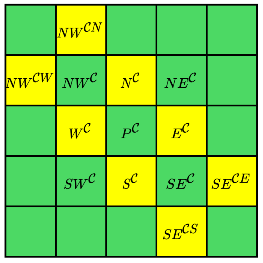
Constructing prediction contexts plays a pivotal role in generating pairs of extreme predictors. In [33], the predictive context of a pixel is defined as the set of pixels in the north, south, west, and east directions. While this approach is straightforward, there is still considerable potential for improving predictor accuracy. This paper expands on the definition of prediction context in [33], as demonstrated in Figure 5. The prediction context $PC\left(P^{\mathcal{C}}\right)$ of the current pixel $P^{\mathcal{C}}$ is defined as

$$PC\left(P^{\mathcal{C}}\right)=\{N^{\mathcal{C}},S^{\mathcal{C}},W^{\mathcal{C}},E^{\mathcal{C}}\}\cup \{D_{\mathcal{C}}^{{\mathcal{R}}_{1}N},D_{\mathcal{C}}^{{\mathcal{R}}_{1}S},D_{\mathcal{C}}^{{\mathcal{R}}_{1}W},D_{\mathcal{C}}^{{\mathcal{R}}_{1}E}\}\cup \{D_{\mathcal{C}}^{{\mathcal{R}}_{2}N},D_{\mathcal{C}}^{{\mathcal{R}}_{2}S},D_{\mathcal{C}}^{{\mathcal{R}}_{2}W},D_{\mathcal{C}}^{{\mathcal{R}}_{2}E}\},$$

(12)

where $D_{\mathcal{C}}^{{\mathcal{R}}_{1}N}$, $D_{\mathcal{C}}^{{\mathcal{R}}_{1}S}$, $D_{\mathcal{C}}^{{\mathcal{R}}_{1}W}$, and $D_{\mathcal{C}}^{{\mathcal{R}}_{1}E}$ represent the pixels to the north, south, west, and east of pixel $D_{\mathcal{C}}^{{\mathcal{R}}_1}$, respectively, and $D_{\mathcal{C}}^{{\mathcal{R}}_{2}N}$, $D_{\mathcal{C}}^{{\mathcal{R}}_{2}S}$, $D_{\mathcal{C}}^{{\mathcal{R}}_{2}W}$, and $D_{\mathcal{C}}^{{\mathcal{R}}_{2}E}$ correspond to the respective directional pixels of $D_{\mathcal{C}}^{{\mathcal{R}}_2}$. Determining $D_{\mathcal{C}}^{{\mathcal{R}}_1}$ and $D_{\mathcal{C}}^{{\mathcal{R}}_2}$ is based on the local complexity calculation algorithm described in Section 3.2. Taking Figure 5 as an example, when $D_{\mathcal{C}}^{R_1}=N{W}^{\mathcal{C}}$ and $D_{\mathcal{C}}^{R_2}=S{E}^{\mathcal{C}}$ are determined according to the inter-channel correlation model, $PC\left(P^{\mathcal{C}}\right)$ can be represented as $PC\left(P^{\mathcal{C}}\right)=\{N^{\mathcal{C}},W^{\mathcal{C}},E^{\mathcal{C}},S^{\mathcal{C}},N{W}^{\mathcal{C}N},N{W}^{\mathcal{C}W},S{E}^{\mathcal{C}E},S{E}^{\mathcal{C}S}\}$.

Once $PC\left(P^{\mathcal{C}}\right)$ is determined, the number of elements in the prediction context set, denoted as n, is calculated, where $card\left(PC\left(P^{\mathcal{C}}\right)\right)=n$, with the $card\left(\right)$ function indicating the number of elements in a set. The elements in $PC\left(P^{\mathcal{C}}\right)$ are sorted in ascending order, represented as ${\tau }_1$, ${\tau }_2$, ${\tau }_3$, …, ${\tau }_{n-2}$, ${\tau }_{n-1}$, ${\tau }_n$, satisfying ${\tau }_1\le {\tau }_2\le {\tau }_3\le \dots \le {\tau }_{n-2}\le {\tau }_{n-1}\le {\tau }_n$. This paper designs three predictors to generate pairs of extreme predictors, namely, $H_h$ and $H_l$, as detailed in

Table 3. Three predictors for generating pairs of extreme predictors $H_h$ and $H_l$.

Predictor Number	1	2	3
$H_h$	${\tau }_n$	$\left[\frac{{\tau }_n+{\tau }_{n-1}}{2}\right]$	$\left[\frac{{\tau }_n+{\tau }_{n-1}+{\tau }_{n-2}}{3}\right]$
$H_l$	${\tau }_1$	$\left[\frac{{\tau }_1+{\tau }_2}{2}\right]$	$\left[\frac{{\tau }_1+{\tau }_2+{\tau }_3}{3}\right]$

. Predictor 1 consists of the most extreme prediction values, namely, the maximum and minimum values in the prediction context set. Predictor 3 comprises the most collaborative prediction values, utilizing the highest number of context elements to generate predictions.

Furthermore, a particular treatment is applied to $H_l$ to avoid redundant data embedding when $H_h$ and $H_l$ are equal, using Equation (4).

3.4. Data Embedding and Extraction

At the data-sending end, we first construct the inter-channel correlation model ${\mathcal{M}}_{\xi 3}$ for the RGB channels. Based on this model, data are embedded channel by channel. For each channel, we calculate the local complexity of each pixel and select pixels with lower complexity for data embedding. The size of the cover color image is $M\times N\times 3$, with each channel being $M\times N$. Based on the characteristic that the sum of the horizontal and vertical positions of pixels is either even or odd, pixels are divided into cross pixels and dot pixels. A two-stage data embedding strategy is executed for cross pixels and dot pixels. For ease of algorithm description, the first stage of data embedding is focused on cross pixels, while the second stage targets dot pixels.

Each pixel $P^{\mathcal{C}}$ undergoes two rounds of data embedding, using high estimates $H_h$ for the first round and low estimates $H_l$ for the second round. The calculation methods for $H_h$ and $H_l$ are detailed in Table 3 of Section 3.3. Initially, the first skewed prediction error histogram is generated from the calculation result of $P^{\mathcal{C}}-H_h$, followed by data embedding using PHS. The embedding method is as follows:

$${\widehat{P}}^{\mathcal{C}}=\left\{\begin{array}{cc}{P}^{\mathcal{C}}+m_1,\hfill & \mathrm{if}{P}^{\mathcal{C}}-H_h=0\hfill \\ P^{\mathcal{C}}+1,\hfill & \mathrm{if}{P}^{\mathcal{C}}-H_h>0\hfill \\ P^{\mathcal{C}},\hfill & \mathrm{otherwise}\hfill \end{array}\right.,$$

(13)

where $m_1$ is the secret data bit to be embedded and $m_1\in \{0,1\}$, with ${\widehat{P}}^{\mathcal{C}}$ representing the pixel value after the first embedding. When the prediction error is zero, one bit of data is embedded, and when the prediction error is positive, the pixel value shifts one unit in the positive direction.

Subsequently, the second skewed prediction error histogram is generated from the calculation result of $P^{\mathcal{C}}-H_l$, followed by data embedding using NHS. The specific embedding method is as follows:

$${\tilde{P}}^{\mathcal{C}}=\left\{\begin{array}{cc}{\widehat{P}}^{\mathcal{C}}-m_2,\hfill & \mathrm{if}{\widehat{P}}^{\mathcal{C}}-H_l=0\hfill \\ {\widehat{P}}^{\mathcal{C}}-1,\hfill & \mathrm{if}{\widehat{P}}^{\mathcal{C}}-H_l<0\hfill \\ {\widehat{P}}^{\mathcal{C}},\hfill & \mathrm{otherwise}\hfill \end{array}\right.,$$

(14)

where $m_2$ represents the secret data bit to be embedded and $m_2\in \{0,1\}$. Here, ${\tilde{P}}^{\mathcal{C}}$ denotes the pixel value after the second data embedding, also known as the marked pixel. When the prediction error is 0, one bit of data is embedded, and the pixel value shifts one unit in the negative direction when the prediction error is negative. The pixel value changes by 0 or +1 because of PHS and by 0 or −1 because of NHS. Consequently, each pixel value can change by at most $\pm 1$ through these two rounds of data embedding.

At the data reception end, to ensure the reversibility of data hiding and extraction, the extraction steps should be performed in reverse order to the embedding steps. Specifically, data are first extracted from dot pixels and then from cross pixels. For dot pixels, secret data extraction is achieved using NHS and low estimate $H_l$, with the extraction formula being

$$m_2=\left\{\begin{array}{cc}0,\hfill & \mathrm{if}{\tilde{P}}^{\mathcal{C}}-H_l=0\hfill \\ 1,\hfill & \mathrm{if}{\tilde{P}}^{\mathcal{C}}-H_l=-1\hfill \end{array}\right.,$$

(15)

and the pixel is restored as

$${\widehat{P}}^{\mathcal{C}}=\left\{\begin{array}{cc}{\tilde{P}}^{\mathcal{C}}+1,\hfill & \mathrm{if}{\tilde{P}}^{\mathcal{C}}-H_l<0\hfill \\ {\tilde{P}}^{\mathcal{C}},\hfill & \mathrm{otherwise}\hfill \end{array}\right..$$

(16)

Subsequently, secret data are extracted using PHS and high estimate $H_h$, with the extraction formula being

$$m_1=\left\{\begin{array}{cc}0,\hfill & \mathrm{if}{\widehat{P}}^{\mathcal{C}}-H_h=0\hfill \\ 1,\hfill & \mathrm{if}{\widehat{P}}^{\mathcal{C}}-H_h=1\hfill \end{array}\right.,$$

(17)

and the pixel is restored as

$$P^{\mathcal{C}}=\left\{\begin{array}{cc}{\widehat{P}}^{\mathcal{C}}-1,\hfill & \mathrm{if}{\widehat{P}}^{\mathcal{C}}-H_h>0\hfill \\ {\widehat{P}}^{\mathcal{C}},\hfill & \mathrm{otherwise}\hfill \end{array}\right..$$

(18)

After the data extraction and pixel recovery for dot pixels, the same method is applied to cross pixels for secret data extraction and pixel recovery.

This paper presents a two-stage embedding process of three RGB channels in Figure 6 to clearly illustrate the data embedding and extraction process. The cover color image I consists of the cover R, G, and B channels. Each channel is divided into cross and dot pixels, i.e., $R_c$, $R_d$, $G_c$, $G_d$, $B_c$, and $B_d$. Then, data embedding is carried out using predictors 1, 2, and 3, resulting in the embedded $R_c^{\prime }$, $R_d^{\prime }$, $G_c^{\prime }$, $G_d^{\prime }$, $B_c^{\prime }$, and $B_d^{\prime }$. Finally, the marked $R^{\prime }$, $G^{\prime }$, and $B^{\prime }$ channels collectively form the marked color image $I^{\prime }$. It is worth mentioning that the final $I^{\prime }$ is the result of selecting the image with minor distortion after data embedding with the three predictors.

3.5. Implementation of the Proposed Method

This paper proposes an RDH framework encompassing both data embedding and extraction processes. Figure 7 details the proposed framework. During the data embedding process, an inter-channel correlation model is constructed based on the correlation among the RGB channels of the cover color image I. Subsequently, local complexity is calculated on a per-pixel basis to identify low-complexity pixels suitable for embedding secret data. Then, pairs of extreme predictors are utilized for skewed histogram shifting, facilitating the embedding of secret data and auxiliary information. This process results in the generation of a marked color image $I’$.

In the data extraction process, the auxiliary information is first extracted from the marked image $I’$. Afterward, the calculation results of local complexity are used to determine which pixels contain embedded data. In pixels within smooth areas, a skewed histogram shifting algorithm is applied to extract the secret data. Finally, the original color image is restored, and the complete secret information is successfully retrieved.

The process of embedding data at the sending end is defined as follows.

(1) Generating location map after preprocessing: Initially, the pixels of the R, G, and B channels are categorized into cross pixels and dot pixels. Pixel pre-processing is implemented to prevent pixel value overflow, either above or below the threshold. For the R, G, and B channels, respective location maps, denoted as ${\mathcal{L}}_r$, ${\mathcal{L}}_g$, and ${\mathcal{L}}_b$, are constructed. The dimensions of each location map correspond to the size of the channel image, that is, $M\times N$. All location maps are initialized with a value of zero. The specific pixel pre-processing method includes adjusting pixel values of 0 to 1 and 255 to 254 in each channel and marking the corresponding position in the location map with a value of 1.

(2) Embedding payload using the improved skewed histogram shifting: We employ arithmetic coding algorithms to compress the data for the location maps ${\mathcal{L}}_r$, ${\mathcal{L}}_g$, and ${\mathcal{L}}_b$. The lengths after compression are denoted as ${\mathcal{\ell }}_{cr}$, ${\mathcal{\ell }}_{cg}$, and ${\mathcal{\ell }}_{cb}$, respectively, with the total compressed length represented by ${\mathcal{\ell }}_c$, satisfying ${\mathcal{\ell }}_c={\mathcal{\ell }}_{cr}+{\mathcal{\ell }}_{cg}+{\mathcal{\ell }}_{cb}$. The payload consists of two parts: the first part is the secret data, and the second part is a bit sequence extracted from the least significant bits (LSBs) of the first ($145+{\mathcal{\ell }}_c$) pixels from the top and bottom rows of the R channel of the cover color image. The secret data are combined with the ($145+{\mathcal{\ell }}_c$) LSBs to form the payload, which is then embedded using our proposed improved skewed histogram shifting.

(3) Embedding auxiliary information and compressed location map: Upon completing the embedding of the payload, we utilize the LSB replacement method to embed auxiliary information into the first 145 pixels of the first row in the red channel. The auxiliary information comprises the following elements: ${\mathcal{\ell }}_{cr}$ (20 bits), ${\mathcal{\ell }}_{cg}$ (20 bits), ${\mathcal{\ell }}_{cb}$ (20 bits), ${\mathcal{M}}_{\xi 3}$ (5 bits), T (8 bits), and the positional information for the endpoints of data embedding across the three channels, with each position occupying 12 bits, totaling 72 bits for the six row and column numbers of the three channels. Following the auxiliary information, we embed the compressed location maps, including the compressed ${\mathcal{L}}_r$, ${\mathcal{L}}_g$, and ${\mathcal{L}}_b$.

The steps involved in the data extraction process at the receiving end are outlined below.

(1) Extracting auxiliary information and compressed location map: To begin, we extract the auxiliary information from the R channel of the marked color image using the LSB replacement, which is located within the first 145 pixels of the first row. Subsequently, utilizing the extracted values of ${\mathcal{\ell }}_{cr}$, ${\mathcal{\ell }}_{cg}$, and ${\mathcal{\ell }}_{cb}$, we proceed to retrieve the compressed location map.

(2) Extracting payload and recovering pixels: We utilize arithmetic coding algorithms to decompress the location maps. Concurrently, based on the inter-channel correlation model ${\mathcal{M}}_{\xi 3}$, we perform information extraction channel by channel and pixel by pixel, thereby restoring the original pixel values.

(3) Recovering color image: From the extracted payload, we separate the secret data and the LSBs. Subsequently, these LSBs are utilized to restore the LSBs of the first 145 pixels in the first row of the R channel. Ultimately, this process completely recovers the cover color image and the secret data.

The complexity of the proposed algorithm is analyzed in terms of time. The algorithm consists of two primary steps: establishing the inter-channel correlation model and implementing the improved skewed histogram shifting. Constructing the inter-channel correlation model involves calculating the covariance between different channels, which has a quadratic time complexity proportional to the total number of pixels in the image. Similarly, the histogram shifting process, which operates on each pixel, exhibits quadratic time complexity.

4. Experimental Results and Analysis

In this section, we conduct a series of experiments to validate the effectiveness of the proposed inter-channel correlation modeling and the improved skewed histogram shifting method for RDH in color images. Initially, we provide detailed information about the experimental datasets and the configuration of the experimental environment. Then, we demonstrate the correctness and efficiency of our algorithm using the USC-SIPI dataset. Subsequently, we perform comparative experiments on the Kodak dataset to further confirm the superiority of our method. Finally, we present a comprehensive performance evaluation and an in-depth analysis of our proposed method.

4.1. Datasets and Experimental Environment Configuration

To substantiate the efficacy of the RDH method proposed in this paper, we meticulously selected two widely recognized datasets for experimental analysis: USC-SIPI (http://sipi.usc.edu/database/database.php?volume=misc (accessed on 20 December 2023)) and Kodak (http://r0k.us/graphics/kodak/ (accessed on 20 December 2023)). The USC-SIPI dataset comprises six color images, each with a resolution of $512\times 512$ pixels, as illustrated in Figure 8. Each image is characterized by its unique texture and pattern, providing an ideal testbed to assess the algorithm’s performance comprehensively. The Kodak dataset consists of 24 color images with dimensions of either $768\times 512$ or $512\times 768$ pixels, encompassing a diverse range of visual content from natural landscapes to urban architecture, thus offering a broad perspective for evaluating the generalization capability of the proposed method.

In the experiments conducted with the USC-SIPI dataset, we adhered to the RDH framework depicted in Figure 8, performing the data embedding and extraction processes on each image. To assess the algorithm’s performance quantitatively, we compared the visual discrepancies between the cover image I and the marked image $I’$ under a fixed data embedding capacity. Concurrently, the data extraction algorithm was employed to verify the consistency between the original cover image and the extracted cover image and the accuracy of the embedded secret data compared to the extracted secret data.

For the Kodak dataset, we replicated the same data hiding and extraction procedures as with the USC-SIPI dataset to ensure the consistency and reproducibility of the experiments. This process validated the effectiveness of our method and demonstrated its stability and reliability when processing various types of images.

The secret data used in our experiments were meticulously generated by a random function, forming a binary string of zeros and ones, to accurately simulate the randomness and diversity found in the real world. Our experimental environment was carefully configured, featuring a macOS Monterey operating system device equipped with an Intel Core i7 processor and 16GB of memory. All experiments were conducted in the stable and extensively supported MATLAB R2020a environment, ensuring the reliability of our results.

We relied on the widely recognized and accepted peak signal-to-noise ratio (PSNR) as our primary metric for the quantitative assessment of image fidelity, measured in decibels (dB). PSNR served as a standard for evaluating the quality comparison between marked and cover images, providing an objective measure to assess the impact of RDH technology on image integrity. This series of experimental configurations allowed us to comprehensively evaluate the performance of the proposed method in various scenarios and, specifically, its impact on image fidelity.

4.2. Comparative Performance Evaluation on USC-SIPI Images

A series of experiments was designed to evaluate the performance differences in color image fidelity among the proposed method and four RDH methods, namely, PEEC [24], CPPAE [30], SHCC [23], and PVOPC [29]. These experiments compared the PSNR values of six USC-SIPI images shown in Figure 8. A higher PSNR value indicated a more remarkable similarity between the marked and original cover images, signifying better image fidelity.

Firstly, we presented the correlation coefficients between the RGB channels of six images depicted in Figure 8 and the inter-channel correlation models established, as shown in

Table 4. The correlation coefficients between the RGB channels and the formulated inter-channel correlation models.

Image	$\mathit{\rho }(\mathit{R},\mathit{G})$	$\mathit{\rho }(\mathit{R},\mathit{B})$	$\mathit{\rho }(\mathit{G},\mathit{B})$	Correlation Model
Lena	0.8786	0.6764	0.9106	${\mathcal{M}}_3$
Baboon	0.3565	0.1237	0.8074	${\mathcal{M}}_3$
Airplane	0.9212	0.8410	0.9380	${\mathcal{M}}_3$
House	0.8070	0.6900	0.9104	${\mathcal{M}}_3$
Peppers	0.2752	0.3952	0.8379	${\mathcal{M}}_1$
Lake	0.8868	0.8271	0.9564	${\mathcal{M}}_3$

. The data in the table reveal variances in the correlations between different channels of the images, which guided us in constructing diverse correlation models. These models enabled the efficient transfer and sharing of information between channels, significantly reducing potential image distortion during the data embedding process. When embedding data into a specific channel, we considered the data from the other channels to adjust our embedding strategy, thereby optimizing the overall image quality. This approach ensured that the images retained high fidelity, even during intensive data embedding.

Subsequently, we embedded secret data of 20,000 bits into the six images in Figure 8 and presented the comparative experimental results in

Table 5. Comparisons in terms of PSNR (dB) on six USC-SIPI color images with the payload of 20,000 bits.

Image	PEEC	CPPAE	SHCC	PVOPC	Proposed
Lena	59.03	60.51	62.07	62.33	62.44
Baboon	57.12	56.81	58.69	58.71	58.78
Airplane	62.16	64.87	65.03	64.71	65.23
House	64.83	65.67	66.05	64.05	66.35
Peppers	56.83	57.12	58.01	62.50	60.82
Lake	59.53	60.44	61.26	62.76	62.85
Average	59.92	60.90	61.85	62.51	62.75

. The experimental results unequivocally demonstrate the superiority of our proposed method. With an embedding capacity of under 20,000 bits, our method consistently outperformed PEEC [24], CPPAE [30], SHCC [23], and PVOPC [29] regarding average PSNR values across the six images. Specifically, when embedding 20,000 bits of data, the average PSNR values of our method surpassed those of PEEC [24], CPPAE [30], SHCC [23], and PVOPC [29] by 2.83, 1.85, 0.9, and 0.24 dB, respectively. These results affirm the superior image fidelity of our method and its ability to maintain high image quality at higher embedding capacities.

This advantage stems from the correlation model established between RGB channels, which enhances the accuracy of local pixel complexity calculations. Moreover, the improved skewed histogram shifting strategy limits the maximum change to one per pixel value during the embedding process, ensuring minimal pixel distortion. However, it is important to note that our method does not always hold an advantage, particularly in certain types of images, such as Peppers, which may be due to their smoother pixel distribution. Future research will focus on algorithmic improvements to achieve better performance across various image types.

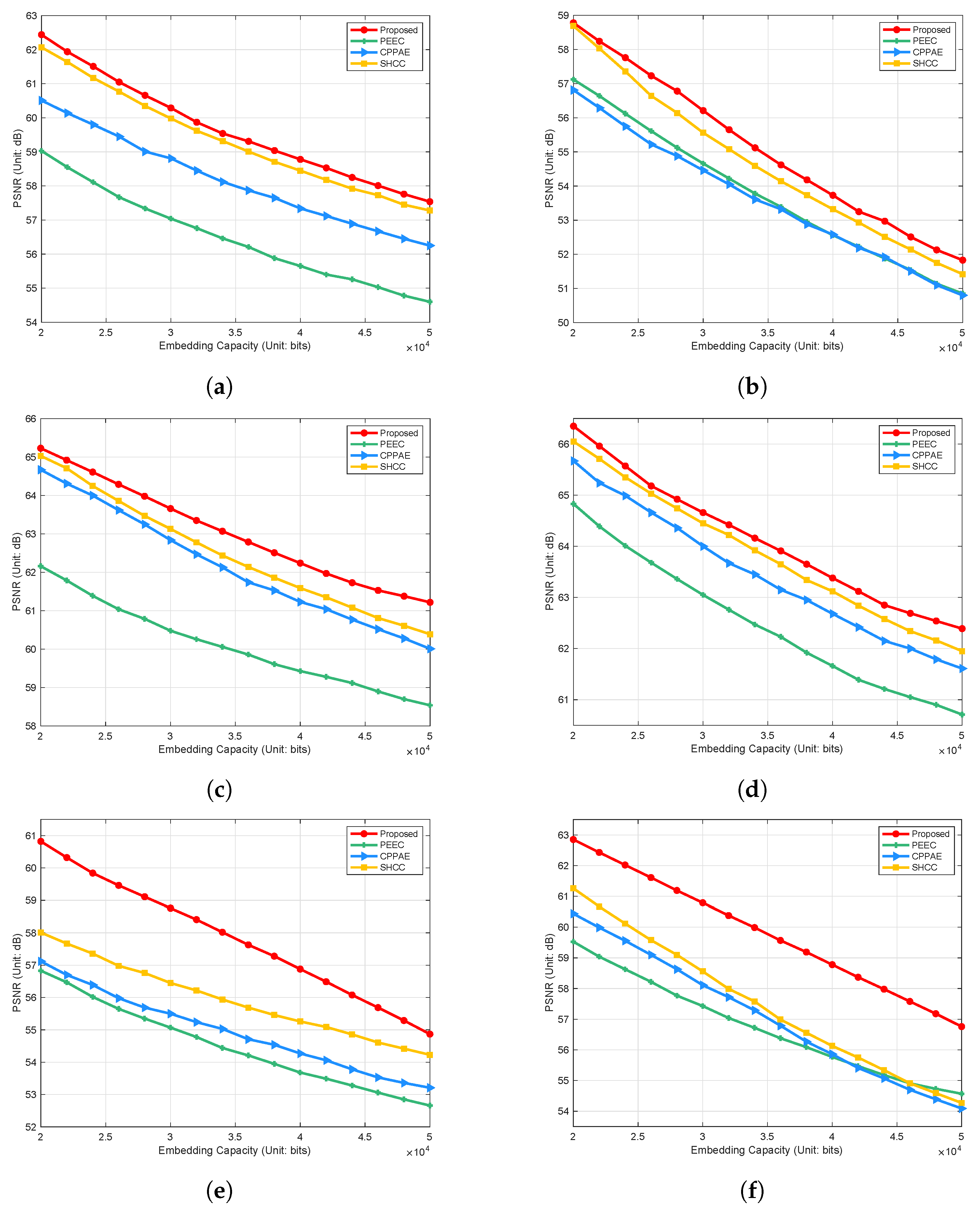
To further validate the performance of our method, the paper begins with an embedding capacity of 20,000 bits. It increases it in increments of 2000 bits, comparing the changes in PSNR values with increasing embedding capacities against PEEC [24], CPPAE [30], SHCC [23], and our method. The results, as shown in Figure 9, indicate that although the PSNR values of our method gradually decrease with the increase in embedding capacity, the rate of decline is slower than those of the other four methods. This result suggests that despite the impact of increased embedding capacity on image quality, our method can effectively control this impact, maintaining a higher level of image fidelity. For instance, at an embedding capacity of 40,000 bits, the PSNR value of our method on the Baboon image is 53.73 dB, which is 1.17, 1.15, and 0.41 dB higher than those of PEEC [24], CPPAE [30], and SHCC [23], respectively. This exceptional performance is attributed to our method’s improved skewed histogram shifting strategy, which provides better error control capabilities, allowing for the maintenance of higher PSNR values even at high embedding capacities.

4.3. Comparative Performance Evaluation on Kodak Images

We meticulously conducted extensive experiments on the Kodak dataset, which comprises 24 images, to evaluate the performance of the proposed method thoroughly. Our comparative experiments between our proposed method and two advanced algorithms, CPPAE [30] and SHCC [23], were designed to compare image quality at an embedding capacity of 50,000 bits, as evaluated by PSNR values. The experimental results, as illustrated in Figure 10, unequivocally demonstrate that the PSNR values of the proposed method surpassed those of the CPPAE [30] and SHCC [23] algorithms for the vast majority of images. This finding underscores the significant advantage of the proposed method in maintaining image quality. Our meticulous analysis suggests that this advantage arises from selecting an appropriate predictive context while generating skewed histograms and constructing more precise extreme predictors, effectively controlling the distortion caused by data embedding. However, it is also observed that on certain types of images, such as the 6th, 13th, 17th, and 23rd images, the PSNR values of the proposed method are slightly lower than those of the SHCC [23]. This may be attributed to the smooth characteristics of these images, which render the advantage of the proposed method in calculating local pixel complexity less pronounced. Overall, the experimental results on the Kodak dataset comprehensively validate the proposed method’s effectiveness and superiority within the RDH field.

4.4. Performance Analysis

In this paper, we present a novel RDH method and conduct a comprehensive performance evaluation. Our method exhibits several advantages in maintaining high PSNR values even as the data embedding capacity increases from 20,000 to 50,000 bits. On the Kodak dataset, our technique sustains superior image quality at an embedding capacity of 50,000 bits. Compared to two leading algorithms, CPPAE [30] and SHCC [23], our technique consistently offers higher PSNR values, highlighting its advantage in image fidelity. The strengths of this paper primarily stem from the established correlation model between the RGB channels of color images, which delves deeply into the inter-channel correlations. The correlation model plays a crucial role in generating the context for local complexity, thereby enhancing the accuracy of local pixel complexity calculations. Additionally, during the skewed histogram generation, we employ an extended predictive context and construct more precise extreme predictors. This meticulous control mechanism effectively controls the distortion caused by data embedding, allowing our method to preserve the visual characteristics of the cover images, especially those with rich textures or complex details. However, the technique also has certain limitations. On specific types of images, particularly those with many smooth areas, the performance of our technique only sometimes prevails. These limitations may be due to our method’s less efficient handling of smooth regions when calculating local pixel complexity. In summary, despite some limitations under certain conditions, the ability of the proposed technique to maintain image quality at high data embedding capacities, along with its robustness in processing complex images, demonstrates its broad application prospects in the field of RDH. This potential impact on the field should inspire further exploration and development.

5. Conclusions

In this paper, we propose an innovative RDH method for color images. This method comprises several key components: a novel inter-channel correlation modeling method, an improved pixel local complexity calculation algorithm, and an improved skewed histogram shifting strategy. The research commences with an in-depth exploration of the inter-channel correlations of RGB channels, upon which a precise inter-channel correlation model is established. Subsequently, we expand the method for calculating pixel local complexity, heightening the algorithm’s sensitivity to image details and enhancing the calculations’ precision. Building on this, we adaptively select the prediction context and design three extreme pixel value predictors. We implement data embedding and extraction through an improved skew histogram shifting strategy, further optimizing the data hiding process. Experimental results confirm that, compared to existing technologies, our proposed method achieves higher PSNR values on most datasets, indicating a significant advantage in maintaining image quality. However, the method’s limitations are evident when dealing with images with smooth pixels. In the future, we will focus on enhancing the robustness and adaptability of our algorithm and explore a broader range of application scenarios, such as privacy protection in medical imaging, hiding sensitive information in secure communications, and embedding copyright information in digital rights management. Our goal is to make a more significant contribution to the field of information security.

References

- Zhang, X.; Liu, M.; Yang, X. Color Image Encryption Algorithm Based on Cross-Spiral Transformation and Zone Diffusion. Mathematics 2023, 11, 3228. [Google Scholar] [CrossRef]
- Moya-Albor, E.; Gomez-Coronel, S.L.; Brieva, J.; Lopez-Figueroa, A. Bio-Inspired Watermarking Method for Authentication of Fundus Images in Computer-Aided Diagnosis of Retinopathy. Mathematics 2024, 12, 734. [Google Scholar] [CrossRef]
- Wang, X.; Zhang, X.; Gao, M.; Tian, Y.; Wang, C.; Iu, H.H.C. A Color Image Encryption Algorithm Based on Hash Table, Hilbert Curve and Hyper-Chaotic Synchronization. Mathematics 2023, 11, 567. [Google Scholar] [CrossRef]
- He, W.; Cai, Z. Reversible Data Hiding Based on Dual Pairwise Prediction-Error Expansion. IEEE Trans. Image Process. 2021, 30, 5045–5055. [Google Scholar] [CrossRef] [PubMed]
- He, W.; Cai, Z. An Insight into Pixel Value Ordering Prediction Based Prediction-error Expansion. IEEE Trans. Inf. Forensic Secur. 2020, 15, 3859–3871. [Google Scholar] [CrossRef]
- Celik, M.; Sharma, G.; Tekalp, A.; Saber, E. Lossless generalized-LSB data embedding. IEEE Trans. Image Process. 2005, 14, 253–266. [Google Scholar] [CrossRef] [PubMed]
- Tian, J. Reversible data embedding using a difference expansion. IEEE Trans. Circuits Syst. Video Technol. 2003, 13, 890–896. [Google Scholar] [CrossRef]
- Alattar, A. Reversible Watermark Using the Difference Expansion of a Generalized Integer Transform. IEEE Trans. Image Process. 2004, 13, 1147–1156. [Google Scholar] [CrossRef] [PubMed]
- Arham, A.; Nugroho, H.A.; Adji, T.B. Multiple layer data hiding scheme based on difference expansion of quad. Signal Process. 2017, 137, 52–62. [Google Scholar] [CrossRef]
- Ni, Z.; Shi, Y.Q.; Ansari, N.; Su, W. Reversible data hiding. IEEE Trans. Circuits Syst. Video Technol. 2006, 16, 354–362. [Google Scholar] [CrossRef]
- Ou, B.; Li, X.; Zhang, W.; Zhao, Y. Improving Pairwise PEE via Hybrid-Dimensional Histogram Generation and Adaptive Mapping Selection. IEEE Trans. Circuits Syst. Video Technol. 2019, 29, 2176–2190. [Google Scholar] [CrossRef]
- He, W.; Xiong, G.; Wang, Y. Reversible Data Hiding Based on Adaptive Multiple Histograms Modification. IEEE Trans. Inf. Forensic Secur. 2021, 16, 3000–3012. [Google Scholar] [CrossRef]
- Thodi, D.M.; Rodriguez, J.J. Expansion Embedding Techniques for Reversible Watermarking. IEEE Trans. Image Process. 2007, 16, 721–730. [Google Scholar] [CrossRef] [PubMed]
- Qiu, Y.; Qian, Z.; Yu, L. Adaptive Reversible Data Hiding by Extending the Generalized Integer Transformation. IEEE Signal Process. Lett. 2016, 23, 130–134. [Google Scholar] [CrossRef]
- Wang, J.; Ni, J.; Zhang, X.; Shi, Y.Q. Rate and Distortion Optimization for Reversible Data Hiding Using Multiple Histogram Shifting. IEEE Trans. Cybern. 2016, 1–12. [Google Scholar] [CrossRef] [PubMed]
- Weinberger, M.; Seroussi, G.; Sapiro, G. The LOCO-I lossless image compression algorithm: Principles and standardization into JPEG-LS. IEEE Trans. Image Process. 2000, 9, 1309–1324. [Google Scholar] [CrossRef] [PubMed]
- Fallahpour, M. Reversible image data hiding based on gradient adjusted prediction. IEICE Electron. Express 2008, 5, 870–876. [Google Scholar] [CrossRef]
- Sachnev, V.; Kim, H.J.; Nam, J.; Suresh, S.; Shi, Y.Q. Reversible Watermarking Algorithm Using Sorting and Prediction. IEEE Trans. Circuits Syst. Video Technol. 2009, 19, 989–999. [Google Scholar] [CrossRef]
- Dragoi, I.C.; Coltuc, D. Local-Prediction-Based Difference Expansion Reversible Watermarking. IEEE Trans. Image Process. 2014, 23, 1779–1790. [Google Scholar] [CrossRef] [PubMed]
- Hwang, H.J.; Kim, S.; Kim, H.J. Reversible data hiding using least square predictor via the LASSO. EURASIP J. Image Video Process. 2016, 2016. [Google Scholar] [CrossRef]
- Kumar, R.; Sharma, D.; Dua, A.; Jung, K.H. A review of different prediction methods for reversible data hiding. J. Inf. Secur. Appl. 2023, 78, 103572. [Google Scholar] [CrossRef]
- Huang, H.; Cai, Z. Duple Color Image Encryption System Based on 3-D Nonequilateral Arnold Transform for IIoT. IEEE Trans. Ind. Informat. 2023, 19, 8285–8294. [Google Scholar] [CrossRef]
- Bhatnagar, P.; Tomar, P.; Naagar, R.; Kumar, R. Reversible Data Hiding scheme for color images based on skewed histograms and cross-channel correlation. In Proceedings of the 2023 International Conference in Advances in Power, Signal, and Information Technology (APSIT), Bhubaneswar, India, 9–11 June 2023. [Google Scholar] [CrossRef]
- Li, J.; Li, X.; Yang, B. Reversible data hiding scheme for color image based on prediction-error expansion and cross-channel correlation. Signal Process. 2013, 93, 2748–2758. [Google Scholar] [CrossRef]
- Chang, Q.; Li, X.; Zhao, Y. Reversible Data Hiding for Color Images Based on Adaptive Three-Dimensional Histogram Modification. IEEE Trans. Circuits Syst. Video Technol. 2022, 32, 5725–5735. [Google Scholar] [CrossRef]
- Kong, Y.; Ke, Y.; Zhang, M.; Su, T.; Ge, Y.; Yang, S. Reversible Data Hiding Based on Multichannel Difference Value Ordering for Color Images. Secur. Commun. Netw. 2022, 2022, 3864480. [Google Scholar] [CrossRef]
- Yao, H.; Qin, C.; Tang, Z.; Tian, Y. Guided filtering based color image reversible data hiding. J. Vis. Commun. Image Represent. 2017, 43, 152–163. [Google Scholar] [CrossRef]
- Mao, N.; He, H.; Chen, F.; Zhu, K. Reversible data hiding of color image based on channel unity embedding. Appl. Intell. 2023, 53, 21347–21361. [Google Scholar] [CrossRef]
- Mao, N.; He, H.; Chen, F.; Qu, L.; Amirpour, H.; Timmerer, C. Reversible data hiding for color images based on pixel value order of overall process channel. Signal Process. 2023, 205, 108865. [Google Scholar] [CrossRef]
- Ou, B.; Li, X.; Zhao, Y.; Ni, R. Efficient color image reversible data hiding based on channel-dependent payload partition and adaptive embedding. Signal Process. 2015, 108, 642–657. [Google Scholar] [CrossRef]
- Kumar, R.; Kumar, N.; Jung, K.H. Color image steganography scheme using gray invariant in AMBTC compression domain. Multidimens. Syst. Signal Process. 2020, 31, 1145–1162. [Google Scholar] [CrossRef]
- Ou, B.; Li, X.; Zhao, Y.; Ni, R.; Shi, Y.Q. Pairwise Prediction-Error Expansion for Efficient Reversible Data Hiding. IEEE Trans. Image Process. 2013, 22, 5010–5021. [Google Scholar] [CrossRef] [PubMed]
- Kim, S.; Qu, X.; Sachnev, V.; Kim, H.J. Skewed Histogram Shifting for Reversible Data Hiding Using a Pair of Extreme Predictions. IEEE Trans. Circuits Syst. Video Technol. 2019, 29, 3236–3246. [Google Scholar] [CrossRef]
Figure 1.
The context used for local complexity calculation. Blue pixels represent the current pixels, while orange pixels represent the complexity context. (a) Four-pixel context. (b) Pairwise context. (c) Extended context.
Figure 2.
Symmetric histogram and skewed histograms. The prediction errors of the pixels are denoted by e. (a) Symmetric histogram. (b) Left-skewed histogram. (c) Right-skewed histogram.
Figure 3.
Consistent pixel value trends across RGB channels at identical locations. (a) Airplane. (b) House.
Figure 4.
The channels used for calculating local complexity. (a) Current channel . (b) Reference channel . (c) Reference channel .
Figure 5.
and its prediction context.
Figure 6.
Two-stage data embedding process of RGB channels.
Figure 7.
An overview of the proposed RDH framework.
Figure 8.
Six USC-SIPI images with a size of . (a) Lena. (b) Baboon. (c) Airplane. (d) House. (e) Peppers. (f) Lake.
Figure 9.
Performance comparison measured with PSNR between PEEC [24], CPPAE [30], SHCC [23], and the proposed method. (a) Lena. (b) Baboon. (c) Airplane. (d) House. (e) Peppers. (f) Lake.
Figure 10.
PSNR performance of the proposed method and existing methods on Kodak images with 50,000 bits of data.