LLE-NET: A Low-Light Image Enhancement Algorithm Based on Curve Estimation

Abstract

Low-light image enhancement is very significant for vision tasks. We introduce Low-light Image Enhancement via Deep Learning Network (LLE-NET), which employs a deep network to estimate curve parameters. Cubic curves and gamma correction are employed for enhancing low-light images. Our research trains a lightweight network to estimate the parameters that determine the correction curve. By the results of the deep learning network, accurate correction curves are confirmed, which are used for the per-pixel correction of RGB channels. The image enhanced by our models closely resembles the input image. To further accelerate the inferring speed of the low-light enhancement model, a low-light enhancement model based on gamma correction is proposed with one iteration. LLE-NET exhibits remarkable inference speed, achieving 400 fps on a single GPU for images sized $640\times 480\times 3$ while maintaining pleasing enhancement quality. The enhancement model based on gamma correction attains an impressive inference speed of 800 fps for images sized $640\times 480\times 3$ on a single GPU.

1. Introduction

Recently, there has been significant development in image-based applications due to continuous development in image-processing algorithms and camera sensors [1]. However, the acquired images are often under-exposed due to inevitable environmental, or technical factors [2], including scene conditions, inadequate illumination or suboptimal camera parameters [3]. Low-light images consistently exhibit low contrast and visibility, presenting challenges for human perception and various high-level visual tasks [4,5], such as object detection [6], object segmentation [7], and object tracking [8]. Low-light image enhancement has a wide range of applications, and reliable low-light image enhancement techniques can improve the visual effects of application scenarios. Enhancing low-light images can effectively enhance the performance of visual simultaneous localization and mapping (SLAM) in low-light underwater conditions [9]. Low-light image enhancement can be used in imaged-based 3D reconstruction in low-light conditions [10]. Enhancing low-light images for lane detection under low-light environments plays a significant role in advanced driver assistance systems (ADAS) [11]. Therefore, the exploration of low-light image enhancement has emerged as a challenging and dynamically evolving research domain [12].

The aims of low-light image enhancement are to enhance the visibility and contrast of low-light images [13]. Numerous conventional methods for enhancing low-light images have been implemented [14,15]. Conventional processing methods typically depend on specific statistical models and assumptions, such as the Retinex model [15] and histogram equalization [16]. Nevertheless, these techniques necessitate parameter adjustments tailored to varying application scenarios, and the imprecise statistical models can easily introduce excessive artifacts [13]. Traditional methods work well for low-contrast images (such as overall darker images); however, they often do not take into account the effects of spatially varing illumination, leading to an unbalanced intensity distribution in local areas [17]. In recent years, a plethora of deep-learning models have surfaced for tasks related to enhancing low-light images. In comparison to conventional methods, these deep-learning approaches offer superior accuracy, robustness, and speed [18]. Despite the substantial performance enhancements brought about by learning-based approaches, a new issue has arisen known as learning bias. This refers to the phenomenon wherein the enhancement results are heavily influenced by the characteristics of the training dataset. In other words, the enhancement effect of low-light image enhancement algorithms using supervised learning is influenced by the low-light image training dataset. The creation of paired low-light image training datasets involves significant subjective factors. To mitigate this constraint, recent exploration has focused on unsupervised learning models utilizing unpaired data. The aim is to develop robust algorithms capable of maintaining generality across diverse real-world scenarios, thus obviating the need for paired data [17]. While learning-based methods often yield satisfactory results, many of them demand substantial computational resources and entail long inference times. Consequently, their suitability for real-time systems or mobile applications is limited [19].

In tasks such as object detection and visual SLAM, low-light image enhancement algorithms based on deep learning commonly serve as preprocessing algorithms for real-time tasks. Thus, low-light image enhancement demands high real-time processing speeds. The bright areas in the enhanced image should be kept from overexposure, and the brightness in dark areas should be increased. The enhanced image should have minimal color distortion. Visual SLAM algorithms are often applied in various application scenarios; hence, it is desired that the low-light enhancement algorithms minimize the influence of paired datasets as much as possible. Therefore, we are looking for low-light image enhancement algorithms that are better suited for image preprocessing in visual tasks related to visual SLAM, with an emphasis on reducing dependency on paired datasets.

Our motivations. To address the problem of image enhancement in low-light environments for visual SLAM, we have designed a low-light image enhancement network. Firstly, in order to improve the algorithm’s adaptability to different scenes, we prioritize using a Zero-shot low-light image enhancement method, avoiding the use of paired training datasets. Secondly, to enhance the inference speed of low-light image enhancement and better meet the real-time requirements of visual SLAM, we have designed a low-light image enhancement method based on gamma correction [20]. Furthermore, to achieve better low-light image enhancement results, we propose a cubic curve enhancement method based on multiple iterations. To fulfill SLAM requirements, our method ensures a close resemblance between the enhanced image and the original input to maintain accuracy.

Our contributions. Our model is inspired by Zero-DCE [21] and LUT-GCE [22]. Different from the Zero-DCE algorithm, we abandon the method of estimating curve parameter maps, and instead, we use a deep-learning network to predict the control parameters of enhancement curves. Unlike LUT-GCE, we improved the network architecture, redesigned the loss function, and additionally introduced a gamma correction-based enhancement method. In comparison to existing open-source deep learning algorithms for enhancing low-light images, our method demonstrates superior performance in both inference speed and resemblance.

Our primary contributions are outlined below:

• A low-light image enhancement model(LLE-NET) based on curve estimation is proposed which estimates the control parameters of enhancement curves. LLE-NET eliminates the need for paired training data, mitigating the risk of overfitting and demonstrating strong generalization across diverse lighting conditions.
• Cubic curves and gamma correction are used in this enhancement method. If computing power permits, using a cubic enhancement curve can achieve fine results. If the computational burden is heavy, a method based on gamma correction for low-light image enhancement can be chosen.
• We conduct extensive experiments to validate the effectiveness of LLE-NET across a wide range of comparison methods and affirm its efficacy.

2. Related Work

In this section, a concise overview of previous works related to low-light image enhancement is introduced, including traditional methods and learning-based methods.

2.1. Traditional Enhancement Methods

Histogram Equalization (HE) is one of the simplest and most commonly used techniques for enhancing low-light images [23]. HE simplifies global statistics by utilizing statistical information across all pixel values, representing them in terms of the density of pixel values [19,24]. Brithness Preserving Bi-Histogram Equalization(BPBHE) was proposed to address the issue of the flattening effect observed in HE methods [25]. Recently, the enhancement of images using HE has been formulated as an optimization problem [23,26]. Gamma correction is applied to color space components with the aim of enhancing contrast [27]. A contrast-limited adaptive histogram equalization (CLAHE) with color correction based on normalized gamma transformation in the Lab color space is suggested for enhancing low-light images [28].

Retinex theory-based methods for enhancing low-light images have attracted significant attention [4,29]. The Retinex model decomposes low-light images into reflection and illumination components [12]. A multi-scale Retinex-based approach utilizing the illumination components is employed for enhancing image contrast [30]. A multi-scale Retinex with color restoration (MSRCR) technique is suggested to address image degradation under foggy weather conditions [31]. An enhanced Retinex algorithm is proposed for enhancing low-light images, addressing issues such as local halo blurring [32].

These traditional methods lack adaptability and may result in significant noise, as well as over- and/or under-enhancement in their outcomes [29]. Global HE methods are based on the grayscale content of the entire image and modify pixels through a transformation function, which can easily lead to local overexposure. Local HE methods consider the equalization of neighborhood pixels by using their histogram intensity statistics. The original image is divided into various sub-blocks in the form of squares or rectangles. Histogram equalization transformation functions are computed at each position by calculating the histogram of neighborhood points, resulting in a checkerboard effect in the enhanced image [23]. Retinex theory-based methods are prone to unnatural and overexposure effects, presenting a challenge in adaptability across various scenes [4]. Furthermore, the computational cost of Retinex algorithms that use traditional iterative optimization for adjusting a single image is high, hindering their application in real-time conditions. Consequently, many deep learning algorithms that improve upon Retinex have been proposed.

2.2. Learning-Based Methods

Recently, learning-based approaches for various vision tasks have been developed. Current low-light image enhancement methods using deep learning can be categorized into four groups: supervised learning, unsupervised learning, semi-supervised learning, and zero-shot learning methods [12].

Supervised learning methods have shown considerable advancements in low-light image enhancement. MBLLEN [33] leverages multi-branch fusion to extract diverse features across various levels, generating the final output image. The SID dataset is obtained by varying the ISO settings while maintaining constant the position of the camera [6,34]. These datasets are often constructed through subjective retouching processes or artificial adjustments of camera parameters [17]. Low-light images are often affected by changes in illumination, color distortion, and noise, making it challenging to determine a singular well-lit reference ground. Consequently, the preference for an enhanced image often varies depending on the user’s choice. Obtaining a true paired image dataset is difficult due to these variations. To mitigate the requirement for extensive training data, large-scale paired low-light datasets are synthesized using efficient low-light simulation techniques. An attention-guided low-light image enhancement approach is proposed, utilizing the synthesized paired simulation dataset [20]. The deep-learning enhancement methods based on Retinex are implemented, such as RetinexNet [35], RUAS [29], KinD [36], SCI [37]. The method based on the exposure prediction model (EPIM) and feature extraction module (FEM) is proposed using hybrid feature weighted fusion strategy [38].

To mitigate the impact of paired training data, unsupervised generative adversarial networks, such as CycleGAN [39] and EnlightenGAN [40] are proposed, eliminating the need for paired low-light image datasets. However, unsupervised GAN-based methods typically require a meticulous selection of unpaired training data. The method based on multi-objective grey wolf optimization is proposed without the need for low-light and normal images as training data [41].

In contrast, zero-shot learning approaches circumvent the need for pre-training and can directly enhance images from input low-light images. Zero-DCE [21] employs pixel-wise and uses high-order curve estimation to dynamically adjust the dynamic range of an input image. RRDNet [42] decomposes the input image into three components, illumination, reflection, and noise. Algorithms based on multi-objective grey wolf optimization introduce transformer structures and attention-guided mechanisms, resulting in larger model sizes compared to Zero-DCE [21], thus leading to poor real-time performance. To expedite inference speed, a single convolutional layer model (SCLM) utilizing effective structural re-parameterization techniques is proposed [19].

Algorithms for low-light image enhancement using supervised learning are often influenced by the training dataset, but they generally perform better in environments similar to the training set. In contrast, unsupervised learning-based low-light image enhancement algorithms avoid the influence of datasets, but many of these algorithms have a heavy computational burden, making them unsuitable for real-time applications, such as EnlightenGAN [40] and the method based on multi-objective grey wolf optimization [41]. The advantage of Zero-shot algorithms is that they avoid the constraint of paired datasets, but the drawback is that they may produce less detailed enhanced images due to the lack of constraints from paired datasets. In practice, current deep learning algorithms have their own strengths and weaknesses based on different evaluation metrics. Generally, evaluations are conducted based on actual application scenarios, such as the requirement for high real-time performance or high enhancement quality. While learning-based methods have delivered satisfactory outcomes, ensuring short inference times is crucial for real-time applications.

3. Proposed Method

The framework of LLE-NET is shown in Figure 1. To accelerate the inference speed, we initially resize the input image to a consistent size $3\times 128\times 128$ pixels using downsampling. Then the resized image is put into the LLE-NET model which predicts Low-light Enhancement curves (LE-curve) trainable parameters. The number of output results predicted by LLE-NET is correlated with the iteration count. Next, the RGB channels of the input image are sequentially enhanced based on the LE-curve defined by the predicted parameters. If the iteration count is greater than 1, the result of the last iterative enhancement image is used as input, and iterative enhancement is performed again using the parameters estimated by LLE-NET until the number of iterations n is reached. We will provide a detailed introduction to the LE-curve, the LLE-NET framework, and the definition of non-reference loss function.

3.1. Low-Light Enhancement Curve

According to the requirements of histogram equalization, if the transformation curve exhibits the following characteristics, it can be utilized as an enhancement curve. Zero-DCE [21] and LUT-GCE [22] have already demonstrated their feasibility.

(1)

The enhancement curve is required to be a continuously ascending function to maintain the contrast between adjacent pixels.

(2)

After normalizing the image, each enhanced pixel value should be confined within the range of [0, 1] to prevent overflow truncation.

(3)

The transformation function should aim for simplicity while remaining differentiable for efficient backpropagation.

We use the cubic curve from reference [22]. The definition of a cubic transformation curve is

$$LE(I\left(\mathit{x}\right);a,t,b,h)=a{(I\left(\mathit{x}\right)-t)}^3+bI\left(\mathit{x}\right)+h,$$

(1)

where $LE\left(I\right(\mathit{x});a,t,b,h)$ represents the enhanced images of the provided input $I\left(\mathit{x}\right)$, $\mathit{x}$ denotes the image pixel, $I\left(\mathit{x}\right)$ is the corresponding pixel value, $a,t,b$ and h are trainable curve parameters. If $a,t,b$ and h are given, the cubic curve will be fully defined.

With the constraints $LE\left(0\right)=0$ and $LE\left(1\right)=1$, we can derive

$$LE=\left\{\begin{array}{cc}\hfill -a{t}^3+h=0& I\left(\mathit{x}\right)=0\hfill \\ \hfill a{(1-t)}^3+b+h=1& I\left(\mathit{x}\right)=1\hfill \end{array}\right..$$

(2)

Furthermore, it can be obtained as formula

$$\left\{\begin{array}{c}\hfill a=\frac{(1-b)}{{(1-t)}^3+t^3}\\ \hfill h=\frac{t^3(1-b)}{{(1-t)}^3+t^3}\end{array}\right..$$

(3)

By computing the derivative of Equation (1), we can obtain that

$$L{E}^{\prime }(I\left(\mathit{x}\right);a,t,b,h)=3a{(I\left(\mathit{x}\right)-t)}^2+b.$$

(4)

When we set $a\ge 0$ and $b\ge 0$, it ensures that the derivative function values are greater than 0. Equation (1) maintains monotonicity to retain the contrast between adjacent pixels.

Next we can reformulate the cubic curve Equation (1) as (5), where $t,b\in [0,1]$ are trainable curve parameters.

$$LE(I\left(\mathit{x}\right);t,b)=\frac{(1-b){(I\left(\mathit{x}\right)-t)}^3}{{(1-t)}^3+t^3}+bI\left(\mathit{x}\right)+\frac{t^3(1-b)}{{(1-t)}^3+t^3}$$

(5)

The LE-curve defined in Equation (1) can be iteratively applied to improve enhancement outcomes in difficult low-light conditions. Equation (6) defines the iterative formula, where n represents the number of iterations. When n is equal to 1, Equation (6) can be degraded to Equation (1).

$$L{E}_{c,n}(L{E}_{c,n-1};a_n,t_n,b_n,h_n)=a_n{(L{E}_{c,n-1}-t_n)}^3+b_{n}L{E}_{c,n-1}+h_n$$

(6)

Only using variables $(t,b)$, Equation (6) can be reformulated as Equation (7).

$$L{E}_{c,n}(L{E}_{c,n-1};t_n,b_n)=\frac{(1-b_n){(L{E}_{c,n-1}-t_n)}^3}{{(1-t_n)}^3+t_n^3}+b_{n}L{E}_{c,n-1}+\frac{t_n^3(1-b_n)}{{(1-t_n)}^3+t_n^3}$$

(7)

To accelerate inference speed, if we set n as equal to 1 using a cubic curve as the enhancement curve, the brightness and contrast of the enhanced image are not very good. So, we cannot simply accelerate the inference speed by reducing the number of iterations as conducted in the Zero-DCE [21] method. However, we try to make our model meet the requirements of real-time applications. In reference [20], low-light images can be converted into normal-light images through a combination of linear and gamma transformations. So, we use gamma correction to enhance low-light images.

The LE-curve based on gamma correction is defined as Equation (7). Ref. [20] shows the synthetic under-exposed image includes gamma transformation and linear transformation. So we add the variable b as the linear transformation.

$$LE{(I\left(\mathit{x}\right);t,b)}^{\left(i\right)}=I^{\left(i\right)}{\left(\mathit{x}\right)}^t+bi\in \{R,G,B\}$$

(8)

To ensure better enhancement performance, LE-cures are applied to the RGB three channels separately. So $\mathit{t}=(t_R,t_G,t_B)$ and $\mathit{b}=(b_R,b_G,b_B)$ are valid.

Even though the gamma correction can enhance the contrast of a low-light image quickly, there is a specific issue that needs clarification. Since the variable t is the exponential part of the gamma function if multiple iterations are performed the derivation will increase rapidly during backpropagation. This makes it is difficult to converge, resulting in training failure. Therefore, the iterative number can only be 1 when using gamma correction enhancement which was verified during subsequent training. Although gamma correction can only be iterated once, it still achieves pleasing enhancement effects.

3.2. LLE-NET

To adapt the algorithm to input images of different resolutions and reduce the computational burden, the input image is downsampled to $3\times 128\times 128$. To keep less change in the low-light regions, each input pixel value should be within the normalized range of [0, 1]. Divide the pixel values represented as integers by 255 to normalize each pixel value to the range of [0, 1]. When enhancing the input image, perform channel-wise operations on the R, G, B channels. Therefore, for channel $i\in \{R,G,B\}$, $\mathit{t}=(t_R,t_G,t_B)$ and $\mathit{b}=(b_R,b_G,b_B)$ should be predicted.

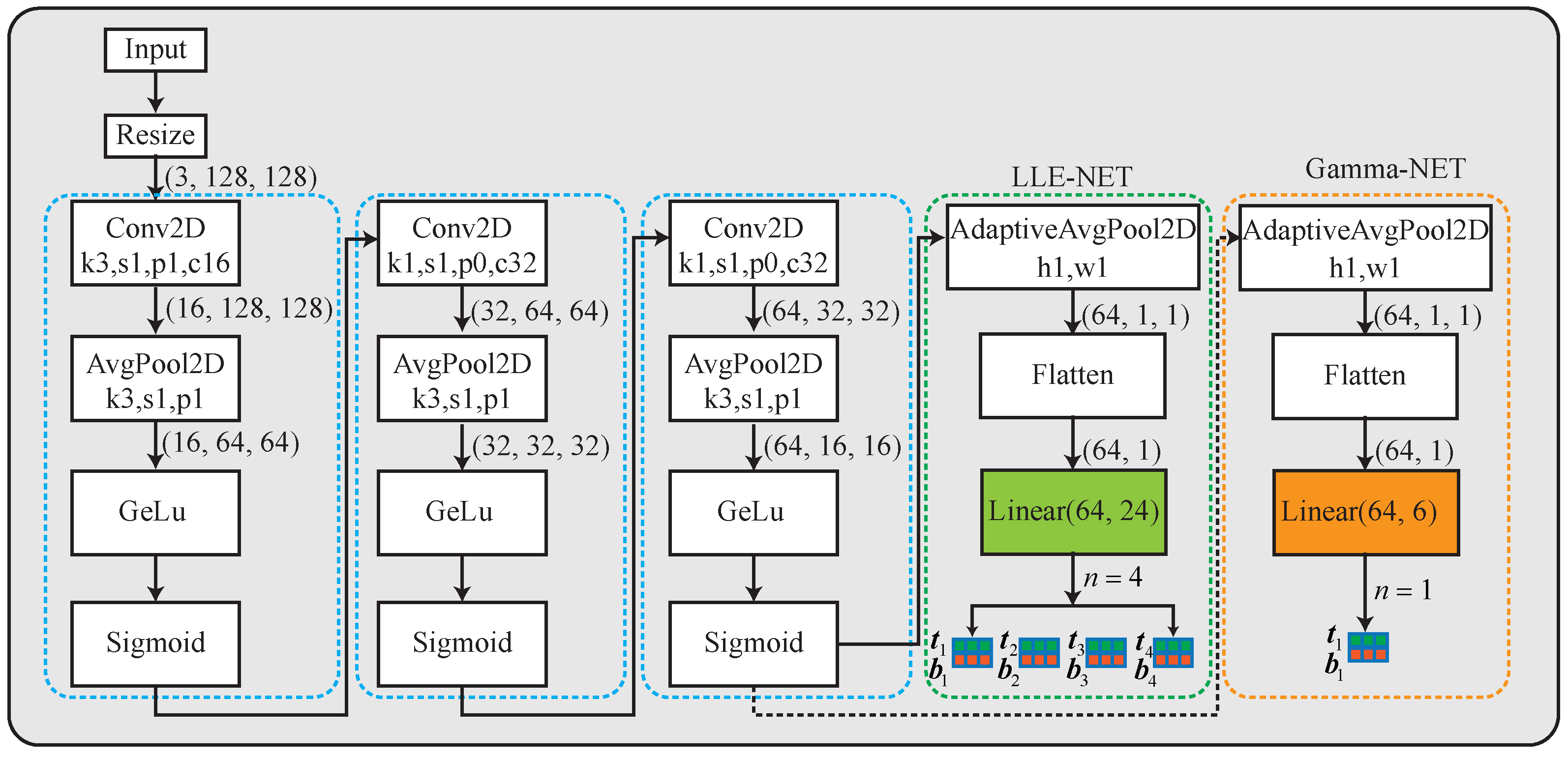
Figure 2 illustrates the detailed structure of LLE-NET when the LE-curve is a cubic curve. The resized images are applied as the input of LLE-NET, which contains three convolutional layers with a simplified channel attention layer [43]. After downsampling, the image is passed through a $3\times 3$ convolution for dimensionality expansion, followed by average pooling for a $1/2$ downsampling operation. The GeLu activation function [44] is utilized in the attention layer to improve gradient preservation. Moreover, a sigmoid operation is applied to ensure that the values of each feature map are within the [0, 1] range. Similar operations continue until the feature map dimension is reduced to (64, 16, 16). Further reduction in dimensionality is achieved through the two-dimensional adaptive average pooling operation(AdaptiveAvgPool2D) to obtain a dimension of (64, 1, 1). After the adaptive average pooling layer, the subsequent layers consist of a flattened layer followed by a linear layer. The predicted result is to generate a $6n$-dimensional vector, where n is iteratively numbers. Parameters ${\{{\mathit{t}}_n,{\mathit{b}}_n\}}_{j=1}^{j=n}$ are used to construct n iteration-specific cubic curves for iterative enhancement. Each iteration applies three LE curves for the three channels in RGB color space. The blue dashed box combined with the green dashed box in the figure constitutes the complete network architecture of LLE-NET with four iterations. The network outputs 24-dimensional data, including $\mathit{t}$ and $\mathit{b}$ for RGB 3 channels used in each iteration. There are six parameters used per iteration with four iterations; the network’s output data are, therefore, 24-dimensional.

After obtaining ${\mathit{t}}_n$ and ${\mathit{b}}_n$ through LLE-NET, plugging them into Equation (7) yields enhancement curves for each iteration. Referring to the algorithm flow in Figure 1, enhance each input image with the LE curve to obtain the image after this iteration’s enhancement until the entire iteration is completed.

3.3. Gamma-NET

We use the same network as LLE-NET when the LE-curve is gamma correction, and set n is equal to 1. If the LE-curve is gamma correction, the enhancement network is remarked as Gamma-NET, as shown in Figure 2. The blue dashed box and the orange dashed box in Figure 2 form the complete structure of the Gamma-NET network. Since the number of iterations is $n=1$, the output dimension of the linear layer is 6. In fact, when n is equal to 1, we can regard Gamma-NET as adaptively estimating gamma correction parameters through a deep-learning network. From the perspective of network architecture, Gamma-NET and LLE-NET only differ in the output of the linear layer. In fact, when the number of iterations for LLE-NET reduces to 1, the network structures of the two are identical with the only difference being in the enhancement curves.

After obtaining the enhancement curve parameters through Gamma-NET, plugging these parameters into Equation (8) yields specific low-light enhancement curves. By enhancing the original input images with these enhancement curves, the final enhanced images can be obtained.

3.4. Non-Reference Loss Function

We define the spatial consistency loss, exposure control loss and color constancy loss to be the same as those in Zero-DCE [21]. The spatial consistency loss $L_{spa}$ maintains the distinction between adjacent regions in both the input and enhanced images, ensuring spatial coherence.

$$L_{spa}={\displaystyle \frac{1}{K}}\sum _{i=1}^K\sum _{j\in \Omega \left(i\right)}{(\mid Y_i-Y_j\mid -\mid I_i-I_j\mid )}^2$$

(9)

In Equation (9), K denotes the count of local areas, and $\Omega \left(i\right)$ represents the four adjacent neighborhoods (top, bottom, left, right) around a specific local area i. Y and I correspond to the average intensity values of the local area in the enhanced and original images, respectively. The dimension of each local region is defined as $4\times 4$ [21]. Figure 3 visually explains the concept of spatial consistency loss.

The exposure control loss $L_{exp}$ seeks to maintain the brightness level of the enhanced images, and it is defined as

$$L_{exp}=\frac{1}{M}\sum _{i=1}^M\mid Y_k-E\mid .$$

(10)

In Equation (10), E is defined as the grayscale value in the RGB color space [45], M denotes the count of distinct local areas each sized $16\times 16$, Y is the mean intensity value of a local region in the enhanced image [21]. Based on experimental evaluations, E is determined to be 0.6.

The color constancy loss $L_{col}$ aims to rectify any possible color shifts in the enhanced image and establish interconnections between RGB channels [21].

$$L_{col}=\sum _{\forall (p,q)\in \epsilon }{(J^p-J^q)}^2,\epsilon =\{(R,G),(R,B),(G,B)\}$$

(11)

In Equation (11), $J^p$ and $J^q$ denote the mean intensity values of the p and q channels, respectively, in the enhanced image [21].

Due to the adoption of curve enhancement instead of pixel-wise enhancement in Zero-DCE [21], the monotonicity of surrounding pixels is maintained according to the properties of curve derivatives. Therefore, we discard the illumination smoothness loss from Zero-DCE [21] and introduce the local contrast loss $L_{con}$. Actually, according to the result of the ablation study, the illumination smoothness loss does not affect the enhancement results.

To make the dark-light regions in the enhanced image clearer, we introduce the local contrast loss $L_{con}$. Figure 4 demonstrates the method used to calculate the local contrast loss. The definition of the local contrast loss is Equation (12)

$$L_{con}=\frac{1}{M}\sum _{i=1}^M\frac{I_{max}-I_{min}}{I_{max}+I_{min}+{10}^{-8}}.$$

(12)

In (12), M denotes the quantity of local regions, each with a size of $4\times 4$. $I_{max}$ and $I_{min}$ correspond to the maximum pixel and minimum pixel values in the enhanced image.

The total loss function is defined as Equation (13), where ${\lambda }_{spa},{\lambda }_{exp},{\lambda }_{col}$, and ${\lambda }_{con}$ are the weights for $L_{spa},L_{exp},L_{col}$ and $L_{con}$.

$$L_{total}={\lambda }_{spa}{L}_{spa}+{\lambda }_{exp}{L}_{exp}+{\lambda }_{col}{L}_{col}+{\lambda }_{con}{L}_{con}$$

(13)

The non-reference loss function for Gamma-Net is the same as LLE-NET, but the loss weights are different from the loss weights of LLE-NET.

4. Experiments

We evaluate LLE-NET and Gamma-Net through experiments conducted on a system comprising an Intel(R) Core(TM) i7-10700k CPU @3.80GHz, 32 GB RAM, and a single NVIDIA GeForce RTX 3060 GPU (with 12 GB memory) running on the PyTorch 1.12 platform. We compare our approach against several state-of-the-art methods, conducting comprehensive qualitative and quantitative assessments to affirm its effectiveness.

4.1. Implementation Details

LLE-NET and Gamma-Net utilize unpaired data for training. Part 1 of SICE [2] comprises 360 multi-exposure images, while the LOL dataset [35] contains 485 training images and 15 test images. The complete training dataset combines the training images from Part 1 of SICE and LOL. To expedite model training, we can randomly choose 400 images from the combined dataset for the training task. Experimental results indicate that a smaller training set yields similar training outcomes compared to the complete training dataset. If there is no strict requirement on training time, it is recommended to use the complete dataset. However, if training time is restricted it is advisable to use random sampling from the complete training dataset as the training dataset. In theory, random sampling should yield enhancement effects similar to those of the complete training dataset. However, practical testing has found that it is best to have over 20% of normal or over-exposed images in the randomly sampled training dataset.

Before training, we first resize training images and testing images to dimensions of $128\times 128\times 3$. The initial filter weights for each layer are initialized using a standard Gaussian distribution with zero mean and a standard deviation of 0.02. We utilize the ADAM optimizer with default parameters, keeping a constant learning rate of ${10}^{-4}$. LLE-NET iteratively enhances four times for input image. The weights ${\lambda }_{spa}, {\lambda }_{col}, {\lambda }_{exp}$ and ${\lambda }_{con}$ are set to 40, 15, 5, and 8 for LLE-NET, respectively. The weights ${\lambda }_{spa}, {\lambda }_{col}, {\lambda }_{exp}$ and ${\lambda }_{con}$ are set to 35, 15, 5, and 8 for Gamma-Net, respectively. The iteration number for LLE-Net is set to 4. The iteration number for Gamma-Net is set to 1, so Gamma-Net is as same as gamma correction. LLE-NET and Gamma-Net adopt the same training dataset. The training dataset in this paper consists of randomly sampled data from the complete training dataset. We selected training weight files with better visual evaluation results as the training outcomes.

4.2. Experimental Evaluation

We contrast our approaches with several state-of-the-art methods: LIME [14], RetinexNet [35], MBLLEN [33], EnlightenGAN [40], RUAS [29], Zero-DCE [21], SCI medium [37]. The images for comparison are generated using publicly available source code with recommended parameters.

Table 1. Computation efficiency of different methods. The trainable parameters for an input image of size $1200\times 900\times 3$, GFLOPs, inference time based on GPU platform in LIME [14] dataset. The best results are highlighted in bold.

Method	Parameters (K) ↓	GFLOPs ↓	Time (s) ↓
RetinexNet [35]	555	587	-
MBLLEN [33]	450	301	21.9512
EnlightenGAN [40]	8000	273	16.1921
RUAS [29]	3.4	3.5	5.5745
Zero-DCE [21]	79	85	3.3182
SCI medium [37]	5.877	188	4.0959
LLE-NET (ours)	76	0.7515	2.9972
Gamma-Net (ours)	75	0.7517	2.8852

compares the trainable parameters and GFLOPs. The GPLOPs are measured when processing $1200\times 900\times 3$ image and the inference time tested in LIME [14] dataset is the running time of different methods. Since RetinexNet has the highest GFLOPs but the slowest computational speed, the runtime of this algorithm is no longer provided. The inference time of Gamma-Net is close to Zero-DCE++ [21]. Compared to other algorithms in Table 1, LLE-NET and Gamma-NET have lower GFLOPs values, giving them a better advantage in terms of runtime. Table 1 presents the runtime of various methods from loading the model to completing the LIME [14] dataset enhancement. LLE-NET exhibits remarkable inference speed, achieving 400 fps on a single GPU for images sized $640\times 480\times 3$ while maintaining pleasing enhancement quality. The enhancement model based on gamma correction attains an impressive inference speed of 800 fps for images sized $640\times 480\times 3$ on a single GPU. The inference time of Gamma-Net based on the GPU platform can reach 0.01s when it processes $1080\times 1920$ images.

We visually compare different methods on the LIME dataset [14] is shown in Figure 5 and Figure 6.

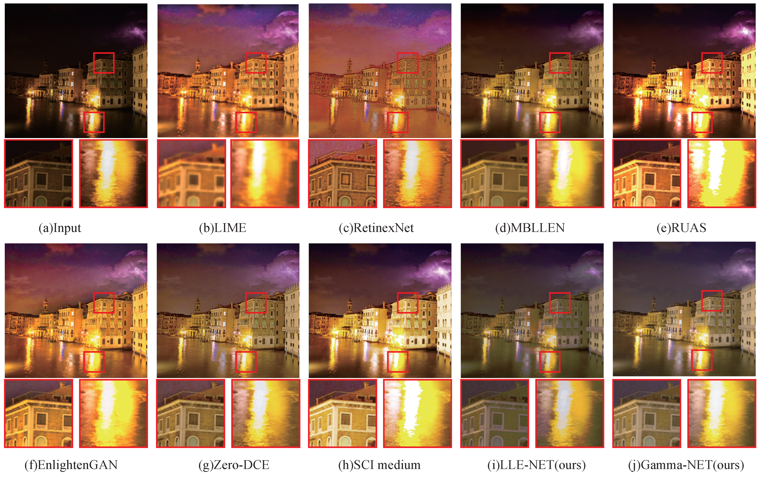
It can be seen from Figure 5 and Figure 6 that LIME [14] cannot recover the building clearly, and the enhanced image of RetinexNet [35] has a painting-like texture. SCI medium [37] and RUAS [29] exhibit uneven exposures, especially, where bright regions in the enhanced image are over-enhanced. Deep learning enhancement algorithms based on the Retinex theory, such as RetinexNet, RUAS, and SCI medium, exhibit overexposure phenomena.

The enhanced images of EnlightenGAN [40] and Zero-DCE [21] appear slight color deviation. The images enhanced by MBLLEN exhibit higher clarity and lesser color distortion compared to LLE-NET. The enhanced image using LLE-NET or Gamma-NET is more similar to the enhanced image using MBLLEN [33]. However, LLE-NET has fewer GFLOPs and faster processing speed compared to MBLLEN. In cases where the enhancement effects are similar, LLE-NET is more suitable for applications with high demands on processing speed. Particularly, LLE-NET retains the advantages of high similarity and low color distortion similar to MBLLEN. Therefore, even if the enhancement effect is slightly inferior to MBLLEN, LLE-NET is still considered more suitable for real-time application scenarios. Compared to Zero-DCE and EnlightenGAN, LLE-NET and Gamma-NET have fewer color distortions. LLE-NET and Gamma-Net tend to under-enhance the low-light images. However, they preserve the bright regions of the input image as faithfully as possible. From the visual effect evaluation, LLE-NET and Gamma-NET are more similar to the original input image.

Qualitative and quantitative evaluations are performed on the standard image set used by previous works including DICM [46] (64 images), LIME [14] (10 images), MEF [47] (17 images), NPE [48] (84 images), VV [49] (24 images). The reference qualitative comparisons are shown in

Table 2. Mean quantitative comparison between our method and state-of-the-art methods on DICM [46], LIME [14], MEF [47], NPE [48], VV [49]. Bold indicates the optimal outcomes.

Dataset	Method	PSNR ↑	SSIM ↑	MAE ↓	LPIPS ↓
DICM	MBLLEN	18.2286	0.7271	1520.6005	0.1981
	RUAS	10.7435	0.6088	6945.4501	0.3509
	EnlightenGAN	13.2887	0.6082	3434.5043	0.2353
	Zero-DCE	14.5836	0.6391	2500.3813	0.2292
	SCI-medium	9.4584	0.5115	8606.4664	0.4096
	LLE-NET	18.7514	0.7180	946.5415	0.2251
	Gamma-Net	14.1608	0.6352	2684.1659	0.2535
LIME	MBLLEN	14.3632	0.5512	3060.0568	0.2800
	RUAS	12.7033	0.5522	4184.1014	0.2390
	EnlightenGAN	10.4526	0.3762	6373.8652	0.3260
	Zero-DCE	12.7292	0.4673	3716.9237	0.3205
	SCI-medium	10.1090	0.3750	7311.8408	0.3533
	LLE-NET	16.6399	0.5587	1462.218	0.3071
	Gamma-Net	13.4485	0.5057	3055.1416	0.2880
MEF	MBLLEN	16.1754	0.5963	1855.8897	0.2510
	RUAS	12.0177	0.5755	4624.5877	0.2633
	EnlightenGAN	12.6525	0.4397	3934.1041	0.2906
	Zero-DCE	13.6976	0.4444	3034.4384	0.2999
	SCI-medium	10.2258	0.3960	6835.2636	0.3595
	LLE-NET	17.5471	0.5581	1225.4604	0.2759
	Gamma-Net	14.0117	0.4812	2702.0425	0.2818
NPE	MBLLEN	19.5104	0.7448	1052.0196	0.1556
	RUAS	10.3375	0.6025	6571.6485	0.3412
	EnlightenGAN	12.6337	0.6552	3783.2525	0.1888
	Zero-DCE	13.8611	0.6519	2817.4149	0.1813
	SCI-medium	9.0282	0.5091	8514.8493	0.3855
	LLE-NET	17.7302	0.7360	1128.3872	0.1813
	Gamma-Net	14.1781	0.545	2575.9487	0.3921
VV	MBLLEN	17.7058	0.7113	1177.6664	0.3196
	RUAS	11.2388	0.6107	5559.8106	0.4134
	EnlightenGAN	11.5388	0.4948	4728.1429	0.5199
	Zero-DCE	13.8369	0.5316	2820.4735	0.4026
	SCI-medium	9.8914	0.4629	7278.1504	0.5279
	LLE-NET	18.1330	0.6238	1042.4784	0.3763
	Gamma-Net	13.6904	0.6814	2819.8596	0.1903
Average	MBLLEN	17.19668	0.67404	1733.2466	0.24086
	RUAS	11.40816	0.58994	5577.1196	0.32156
	EnlightenGAN	12.11326	0.51482	4450.7738	0.31212
	Zero-DCE	13.74168	0.54686	2977.9263	0.2867
	SCI-medium	9.98208	0.42828	7373.39696	0.40196
	LLE-NET	17.76032	0.63892	1161.0171	0.27314
	Gamma-Net	13.8979	0.5697	2767.43166	0.28114

which gives the detailed results of five datasets in terms of Peaking Signal-to-Noise Ratio (PSNR,dB), Structural similarity (SSIM), Mean Absolute Error (MAE), and Learned Perceptual Image Patch Similarity (LPIPS) [50]. The detailed results in five datasets are presented in Table 2. The MBLLEN algorithm excels in SSIM and LIPIS metrics, whereas the LLE-NET algorithm outperforms in terms of PSNR and MAE metrics. It can be concluded that images enhanced using LLE-NET have better performance in terms of similarity and smaller color distortion, and are especially suitable for applications such as SLAM. The evaluation metric results are consistent with the visual assessment. We can conclude that the LLE-NET and Gamma-NET algorithms ensure enhancement while maximizing similarity to low-light images. Gamma-NET and Zero-DCE have similar evaluation indicators. It can be seen that using Gamma-NET can achieve similar effects to Zero-DCE. The inference speed of Gamma-NET increases obviously compared to Zero-DCE. Because there is no established ground truth for the enhanced images, using reference qualitative methods cannot fully evaluate the quality of enhanced images. Therefore, non-reference qualitative methods are introduced.

Non-reference qualitative comparisons of the Perceptual index (PI) [51] and Natural Image Quality Evaluator (NIQE) [52] on five datasets are listed in

Table 3. Perceptual Index (PI) ↓/Naturalness Image Quality Evaluator (NIQE) ↓ on different datasets. Bold means the best results.

Method	Average	DICM	LIME	MEF	NPE	VV
MBLLEN	3.84/4.43	3.75/4.20	3.63/4.50	3.91/4.73	3.43/4.54	4.48/4.18
RUAS	3.54/4.59	3.83/4.78	3.09/4.23	2.77/3.69	3.87/5.68	4.14/4.60
EnlightenGAN	3.34/3.90	3.11/3.48	2.83/3.66	2.45/3.22	2.96/4.11	5.35/5.01
Zero-DCE	2.94/3.60	3.08/3.60	3.00/3.95	2.43/3.28	2.86/3.93	3.33/3.22
SCI-medium	3.03/3.65	3.51/3.79	2.99/4.18	2.56/3.44	2.56/3.44	3.55/3.42
LLE-NET	3.15/3.80	3.19/3.75	3.00/3.95	2.88/3.52	3.09/4.39	3.61/3.39
Gamma-Net	3.11/3.73	3.17/3.69	3.19/3.99	2.76/3.38	3.52/3.32	2.96/4.25

. As we can see, Zero-DCE [21] obtains the best score in terms of PI and NIQE. LLE-NET and Gamma-Net achieve good scores compared to other methods. Since non-reference qualitative comparison is closer to the judgment standard of the human eye, taking into account the content of Figure 5 and Figure 6, Zero-DCE exhibits superior performance in contrast and saturation of the enhanced image. However, there is noticeable color distortion present as well. Color distortion is detrimental to tasks such as vision SLAM. Since algorithms cannot excel in all metrics, we need to choose low-light image enhancement algorithms according to different requirements of tasks.

To assess and contrast the performance and efficiency of different methods, Figure 7 shows the relationship between PI and GFLOPs. The enhanced performance of Gamma-Net is similar to Zero-DCE [21]. LLE-NET and Gamma-Net, using global lookup tables for high-resolution images, can accelerate inferring speed. Combining the runtime data in Table 1, it can be observed that LLE-NET runs at a higher frame rate than Zero-DCE, while Gamma-NET surpasses both LLE-NET and Zero-DCE. In fact, considering the frame rate processing indicator, Gamma-NET is essentially twice as fast as LLE-NET and Zero-DCE.

Limitations. The LLE-NET and Gamma-NET algorithms do not perform exceptionally well in non-reference metric evaluation. In fact, visually, images enhanced using these two methods tend to have an overall dark brightness. The enhanced image’s texture details are not clear compared to MBLLEN, and they are noticeably affected by noise. The contrast and color saturation of the enhanced images are lacking compared to the Zero-DCE and EnlightenGAN methods. Since a pixel-wise mapping similar to the Zero-DCE algorithm was not employed, the enhanced images exhibit the drawbacks of traditional image enhancement algorithms, such as low contrast and relatively low color saturation. Due to the absence of a noise filtering module, noise in the input image directly affects the effectiveness of the enhanced image. It may be beneficial to introduce a noise removal module while enhancing images to further improve the quality of the enhanced images.

Although our methods can not achieve the best score in every index, our approach demonstrates strong competitiveness in overall performance, particularly given its similarity to input images and its inference speed.

4.3. Ablation Study

In order to evaluate the impact of each loss component, the results of LLE-NET trained using different combinations of loss weights are shown in Figure 8. Figure 8b shows the enhancement image by the weights combination of $(40,15,5,8)$. During the ablation study process, we found that setting the weight of $L_{spa}$ to zero is not feasible. Therefore, we decided to decrease the weight of $L_{spa}$ to 30. From Figure 8b,c, $L_{spa}$ reduce noise and preserve the overall contrast of the enhanced image. From Figure 8b,d, $L_{col}$ prevents the color deviation of the enhanced image. From Figure 8b,e, $L_{exp}$ improves the overall exposure of enhanced images. From Figure 8b,f, $L_{con}$ improves the local contrast of the enhanced images. Besides, the value of $L_{con}$ influences the value of $L_{spa}$. Figure 8 illustrates the significant contribution of each loss in achieving the final enhancement result.

Table 4. Perceptual Index (PI) ↓/Naturalness Image Quality Evaluator (NIQE) ↓ on different combinations. Bold means the best results.

	(40, 15, 5, 8)	(30, 15, 5, 8)	(40, 0, 5, 8)	(40, 15, 0, 8)	(40, 15, 5, 0)
PI↓	2.9957	3.21121	3.1610	3.0962	3.0469
NIQE↓	3.948	4.2345	4.2512	3.9505	3.9963

presents the metrics of non-reference qualitative comparisons. These metrics show the significance of the divergence loss function.

4.4. Effect of Parameter Setting

The parameter E is included in the loss function $L_{exp}$, as shown in Equation (10). During training, it was observed that this parameter affects the enhancement results. By comparing the parameter values set to 0.4, 0.5, 0.6, 0.7, it was observed that a generally superior effect is attained when E is configured to 0.6. Figure 9 presents qualitative comparisons for different values of E in LLE-NET. It can be observed that as the value of E increases, there is a corresponding rise in image brightness. However, when $E=0.7$, noticeable noise artifacts appear in the enlarged images.

The impact of training epochs on this research was investigated, revealing that higher epochs do not necessarily yield better results. It was observed that setting the epoch value too high leads to increased image noise and loss of details, while lower epochs result in less noticeable enhancements in image brightness. Thus, it is advisable not to opt for higher epoch values during training. The experiments found that typically, setting the epoch value to below 50 is sufficient, with around 20 epochs often meeting the requirements. Figure 10 illustrates the training results for different epochs in Gamma-NET. It can be seen that at epoch 3, enhancement in dark regions is achieved, with further improvement at epoch 8. However, by epoch 11, noise becomes noticeable in the darker regions of the image. It was noted that setting the epoch value too high results in noise becoming a significant part of the enhanced image, thus it is recommended to use slightly lower epoch values in practical network applications.

4.5. Effect of Training Data

The training dataset for the LLE-NET network and Gamma-NET influences the enhancement results. Figure 11 illustrates the impact of various datasets on enhancement outcomes. Two datasets were used in this research: the LOL dataset [35] and the first part of the SCIE dataset [2]. Experimental results revealed a significant influence of the training set on data augmentation results. Figure 11b shows the results after training with the LOL dataset, indicating lower overall image brightness and poor enhancement in dark areas. The first part of the SCIE dataset includes a total of 3021 images which are divided into 360 groups with and without reference assessment, each group containing images with varying brightness levels. A composite training set was assembled by merging images from both the LOL and the initial section of the SCIE dataset, culminating in a sum of 3506 images, as shown in Figure 11c. It can be observed that training with a combination of low and high-light images can effectively improve enhancement results. During training, it was found that one complete training cycle takes about 30 min. To speed up training, a random selection of 400 images was used for training, as shown in Figure 11d. It was found that this approach yielded training results comparable to using the complete training set. Therefore, in scenarios where training time is a constraint, constructing a dataset with a combination of low and high-light images and training with a smaller random subset of images can still achieve good enhancement results. The dataset is composed of randomly selected images and must include approximately $20\%$ of images that are either normal or over-exposed. Considering algorithm applicability and contrast enhancement of the enhanced images, this study recommends using a combined dataset of low and high-light images for training and suggests training with a random sample of 200–500 images. For example, training with 200 images takes approximately 4 min.

5. Conclusions

In this research, the framework of LLE-NET and Gamma-NET is proposed without paired training datasets, and an appropriate loss function is defined. By comparing with existing algorithms, we concluded that using LLE-NET can achieve better image enhancement effects. Firstly, the LLE-NET and Gamma-NET algorithms achieve comparable results to MBLLEN with smaller models, meeting the requirements for real-time applications. Secondly, compared to the Zero-DCE and EnlightenGAN algorithms, LLE-NET and Gamma-NET algorithms exhibit fewer color distortions and better image similarity. They achieve optimal results in PSNR and MAE evaluation metrics. Therefore, the algorithms overall meet the requirements of our design, providing higher processing speeds and image similarity while meeting enhancement requirements. In terms of algorithm processing speed evaluation, when the input image size is $640\times 480$, the processing speed of LLE-NET can reach 400 fps, and Gamma-NET can reach 800 fps.

Despite the algorithms performing well in some aspects, limitations still exist. The lack of paired training datasets makes it challenging to perform denoising simultaneously with image enhancement using Zero-shot methods. Therefore, researching network structures that simultaneously remove noise and enhance low-light images holds greater application value.

References

- Moran, S.; Marza, P.; McDonagh, S.; Parisot, S.; Slabaugh, G. Deeplpf: Deep local parametric filters for image enhancement. In Proceedings of the IEEE/CVF Conference on Computer Vision and Pattern Recognition, Seattle, WA, USA, 13–19 June 2020; pp. 12826–12835. [Google Scholar]
- Cai, J.; Gu, S.; Zhang, L. Learning a deep single image contrast enhancer from multi-exposure images. IEEE Trans. Image Process. 2018, 27, 2049–2062. [Google Scholar] [CrossRef] [PubMed]
- Yang, S.; Zhou, D.; Cao, J.; Guo, Y. LightingNet: An integrated learning method for low-light image enhancement. IEEE Trans. Comput. Imaging 2023, 9, 29–42. [Google Scholar] [CrossRef]
- Wu, W.; Weng, J.; Zhang, P.; Wang, X.; Yang, W.; Jiang, J. Uretinex-net: Retinex-based deep unfolding network for low-light image enhancement. In Proceedings of the IEEE/CVF Conference on Computer Vision and Pattern Recognition, New Orleans, LA, USA, 18–24 June 2022; pp. 5901–5910. [Google Scholar]
- Li, C.; Qu, X.; Gnanasambandam, A.; Elgendy, O.A.; Ma, J.; Chan, S.H. Photon-limited object detection using non-local feature matching and knowledge distillation. In Proceedings of the IEEE/CVF International Conference on Computer Vision, Montreal, BC, Canada, 11–17 October 2021; pp. 3976–3987. [Google Scholar]
- Wang, W.; Wang, X.; Yang, W.; Liu, J. Unsupervised face detection in the dark. IEEE Trans. Pattern Anal. Mach. Intell. 2022, 45, 1250–1266. [Google Scholar] [CrossRef] [PubMed]
- Gao, H.; Guo, J.; Wang, G.; Zhang, Q. Cross-domain correlation distillation for unsupervised domain adaptation in nighttime semantic segmentation. In Proceedings of the IEEE/CVF Conference on Computer Vision and Pattern Recognition, New Orleans, LA, USA, 18–24 June 2022; pp. 9913–9923. [Google Scholar]
- Ye, J.; Fu, C.; Zheng, G.; Paudel, D.P.; Chen, G. Unsupervised domain adaptation for nighttime aerial tracking. In Proceedings of the IEEE/CVF Conference on Computer Vision and Pattern Recognition, New Orleans, LA, USA, 18–24 June 2022; pp. 8896–8905. [Google Scholar]
- Xin, Z.; Wang, Z.; Yu, Z.; Zheng, B. ULL-SLAM: Underwater low-light enhancement for the front-end of visual SLAM. Front. Mar. Sci. 2023, 10, 1133881. [Google Scholar] [CrossRef]
- Su, Y.; Wang, J.; Wang, X.; Hu, L.; Yao, Y.; Shou, W.; Li, D. Zero-reference deep learning for low-light image enhancement of underground utilities 3D reconstruction. Autom. Constr. 2023, 152, 104930. [Google Scholar] [CrossRef]
- Song, S.; Chen, W.; Liu, Q.; Hu, H.; Huang, T.; Zhu, Q. A novel deep learning network for accurate lane detection in low-light environments. Proc. Inst. Mech. Eng. Part D J. Automob. Eng. 2022, 236, 424–438. [Google Scholar] [CrossRef]
- Tang, H.; Zhu, H.; Fei, L.; Wang, T.; Cao, Y.; Xie, C. Low-Illumination image enhancement based on deep learning techniques: A brief review. Photonics 2023, 10, 198. [Google Scholar] [CrossRef]
- Peng, B.; Zhang, X.; Lei, J.; Zhang, Z.; Ling, N.; Huang, Q. LVE-S2D: Low-light video enhancement from static to dynamic. IEEE Trans. Circuits Syst. Video Technol. 2022, 32, 8342–8352. [Google Scholar] [CrossRef]
- Guo, X.; Li, Y.; Ling, H. LIME: Low-Light Image Enhancement via Illumination Map Estimation. IEEE Trans. Image Process. 2017, 26, 982–993. [Google Scholar] [CrossRef]
- Jobson, D.J.; Rahman, Z.u.; Woodell, G.A. A multiscale retinex for bridging the gap between color images and the human observation of scenes. IEEE Trans. Image Process. 1997, 6, 965–976. [Google Scholar] [CrossRef]
- Arici, T.; Dikbas, S.; Altunbasak, Y. A histogram modification framework and its application for image contrast enhancement. IEEE Trans. Image Process. 2009, 18, 1921–1935. [Google Scholar] [CrossRef] [PubMed]
- Kim, W. Low-light image enhancement: A comparative review and prospects. IEEE Access 2022, 10, 84535–84557. [Google Scholar] [CrossRef]
- Li, C.; Guo, C.; Han, L.; Jiang, J.; Cheng, M.M.; Gu, J.; Loy, C.C. Low-light image and video enhancement using deep learning: A survey. IEEE Trans. Pattern Anal. Mach. Intell. 2021, 44, 9396–9416. [Google Scholar] [CrossRef] [PubMed]
- Zhang, Y.; Teng, B.; Yang, D.; Chen, Z.; Ma, H.; Li, G.; Ding, W. Learning a Single Convolutional Layer Model for Low Light Image Enhancement. IEEE Trans. Circuits Syst. Video Technol. 2023. [Google Scholar] [CrossRef]
- Lv, F.; Li, Y.; Lu, F. Attention guided low-light image enhancement with a large scale low-light simulation dataset. Int. J. Comput. Vis. 2021, 129, 2175–2193. [Google Scholar] [CrossRef]
- Li, C.; Guo, C.; Loy, C.C. Learning to enhance low-light image via zero-reference deep curve estimation. IEEE Trans. Pattern Anal. Mach. Intell. 2021, 44, 4225–4238. [Google Scholar] [CrossRef] [PubMed]
- Wu, C.; Dong, J.; Tang, J. LUT-GCE: Lookup Table Global Curve Estimation for Fast Low-light Image Enhancement. arXiv 2023, arXiv:2306.07083. [Google Scholar]
- Dhal, K.G.; Das, A.; Ray, S.; Gálvez, J.; Das, S. Histogram equalization variants as optimization problems: A review. Arch. Comput. Methods Eng. 2021, 28, 1471–1496. [Google Scholar] [CrossRef]
- Ibrahim, H.; Kong, N.S.P. Brightness preserving dynamic histogram equalization for image contrast enhancement. IEEE Trans. Consum. Electron. 2007, 53, 1752–1758. [Google Scholar] [CrossRef]
- Chen, S.D.; Ramli, A.R. Preserving brightness in histogram equalization based contrast enhancement techniques. Digit. Signal Process. 2004, 14, 413–428. [Google Scholar] [CrossRef]
- Dhal, K.G.; Sen, M.; Das, S. Cuckoo search-based modified bi-histogram equalisation method to enhance the cancerous tissues in mammography images. Int. J. Med. Eng. Inform. 2018, 10, 164–187. [Google Scholar]
- Muniraj, M.; Dhandapani, V. Underwater image enhancement by modified color correction and adaptive Look-Up-Table with edge-preserving filter. Signal Process. Image Commun. 2023, 113, 116939. [Google Scholar] [CrossRef]
- Shi, Z.; Feng, Y.; Zhao, M.; Zhang, E.; He, L. Normalised gamma transformation-based contrast-limited adaptive histogram equalisation with colour correction for sand–dust image enhancement. IET Image Process. 2020, 14, 747–756. [Google Scholar] [CrossRef]
- Liu, R.; Ma, L.; Zhang, J.; Fan, X.; Luo, Z. Retinex-inspired unrolling with cooperative prior architecture search for low-light image enhancement. In Proceedings of the IEEE/CVF Conference on Computer Vision and Pattern Recognition, Nashville, TN, USA, 20–25 June 2021; pp. 10561–10570. [Google Scholar]
- Bao, S.; Ma, S.; Yang, C. Multi-scale retinex-based contrast enhancement method for preserving the naturalness of color image. Opt. Rev. 2020, 27, 475–485. [Google Scholar] [CrossRef]
- Zhang, W.; Dong, L.; Pan, X.; Zhou, J.; Qin, L.; Xu, W. Single Image Defogging Based on Multi-Channel Convolutional MSRCR. IEEE Access 2019, 7, 72492–72504. [Google Scholar] [CrossRef]
- Tian, F.; Wang, M.; Liu, X. Low-Light mine image enhancement algorithm based on improved Retinex. Appl. Sci. 2024, 14, 2213. [Google Scholar] [CrossRef]
- Lv, F.; Lu, F.; Wu, J.; Lim, C. MBLLEN: Low-Light Image/Video Enhancement Using CNNs. In BMVC; Northumbria University: Newcastle upon Tyne, UK, 2018; Volume 220, p. 4. [Google Scholar]
- Chen, C.; Chen, Q.; Xu, J.; Koltun, V. Learning to see in the dark. In Proceedings of the IEEE Conference on Computer Vision and Pattern Recognition, Salt Lake City, UT, USA, 18–23 June 2018; pp. 3291–3300. [Google Scholar]
- Chen, W.; Wang, W.; Yang, W.; Liu, J. Deep retinex decomposition for low-light enhancement. In British Machine Vision Conference; British Machine Vision Association: Glasgow, UK, 2018. [Google Scholar]
- Zhang, Y.; Guo, X.; Ma, J.; Liu, W.; Zhang, J. Beyond brightening low-light images. Int. J. Comput. Vis. 2021, 129, 1013–1037. [Google Scholar] [CrossRef]
- Ma, L.; Ma, T.; Liu, R.; Fan, X.; Luo, Z. Toward fast, flexible, and robust low-light image enhancement. In Proceedings of the IEEE/CVF Conference on Computer Vision and Pattern Recognition, New Orleans, LA, USA, 18–24 June 2022; pp. 5637–5646. [Google Scholar]
- Hui, Y.; Wang, J.; Shi, Y.; Li, B. Low-light Image Enhancement Algorithm Based on Exposure Prediction and Hybrid Feature Weighted Fusion Strategy. Proc. J. Phys. Conf. Ser. 2022, 2281, 012017. [Google Scholar] [CrossRef]
- Zhu, J.Y.; Park, T.; Isola, P.; Efros, A.A. Unpaired image-to-image translation using cycle-consistent adversarial networks. In Proceedings of the IEEE International Conference on Computer Vision, Venice, Italy, 22–29 October 2017; pp. 2223–2232. [Google Scholar]
- Jiang, Y.; Gong, X.; Liu, D.; Cheng, Y.; Fang, C.; Shen, X.; Yang, J.; Zhou, P.; Wang, Z. Enlightengan: Deep light enhancement without paired supervision. IEEE Trans. Image Process. 2021, 30, 2340–2349. [Google Scholar] [CrossRef] [PubMed]
- Hui, Y.; Jue, W.; Li, B.; Shi, Y. Low light image enhancement algorithm based on improved multi-objective grey wolf optimization with detail feature enhancement. J. King Saud Univ.-Comput. Inf. Sci. 2023, 35, 101666. [Google Scholar] [CrossRef]
- Zhu, A.; Zhang, L.; Shen, Y.; Ma, Y.; Zhao, S.; Zhou, Y. Zero-shot restoration of underexposed images via robust retinex decomposition. In Proceedings of the 2020 IEEE International Conference on Multimedia and Expo (ICME), London, UK, 6–10 July 2020; pp. 1–6. [Google Scholar]
- Chen, L.; Chu, X.; Zhang, X.; Sun, J. Simple baselines for image restoration. In European Conference on Computer Vision; Springer: Cham, Switzerland, 2022; pp. 17–33. [Google Scholar]
- Hendrycks, D.; Gimpel, K. Gaussian error linear units (gelus). arXiv 2016, arXiv:1606.08415. [Google Scholar]
- Mertens, T.; Kautz, J.; Van Reeth, F. Exposure fusion: A simple and practical alternative to high dynamic range photography. In Computer Graphics Forum; Wiley Online Library: Oxford, UK, 2009; Volume 28, pp. 161–171. [Google Scholar]
- Lee, C.; Lee, C.; Kim, C.S. Contrast enhancement based on layered difference representation of 2D histograms. IEEE Trans. Image Process. 2013, 22, 5372–5384. [Google Scholar] [CrossRef] [PubMed]
- Ma, K.; Zeng, K.; Wang, Z. Perceptual quality assessment for multi-exposure image fusion. IEEE Trans. Image Process. 2015, 24, 3345–3356. [Google Scholar] [CrossRef] [PubMed]
- Wang, S.; Zheng, J.; Hu, H.M.; Li, B. Naturalness Preserved Enhancement Algorithm for Non-Uniform Illumination Images. IEEE Trans. Image Process. 2013, 22, 3538–3548. [Google Scholar] [CrossRef]
- Vonikakis, V. Busting Image Enhancement and Tonemapping Algorithms. Available online: https://sites.google.com/site/vonikakis/datasets (accessed on 1 January 2021).
- Zhang, R.; Isola, P.; Efros, A.A.; Shechtman, E.; Wang, O. The unreasonable effectiveness of deep features as a perceptual metric. In Proceedings of the 2018 IEEE/CVF Conference on Computer Vision and Pattern Recognition, Salt Lake City, UT, USA, 18–23 June 2018; pp. 586–595. [Google Scholar]
- Blau, Y.; Michaeli, T. The perception-distortion tradeoff. In Proceedings of the 2018 IEEE/CVF Conference on Computer Vision and Pattern Recognition, Salt Lake City, UT, USA, 18–23 June 2018; pp. 6228–6237. [Google Scholar]
- Mittal, A.; Soundararajan, R.; Bovik, A.C. Making a “Completely Blind” Image Quality Analyzer. IEEE Signal Process. Lett. 2013, 20, 209–212. [Google Scholar] [CrossRef]
Figure 1.
Framework of LLE-NET. LLE-NET is designed to predict parameters for Light-Enhancement curves(LE-curve). LE-curves are applied to iteratively enhance a given image.
Figure 2.
Architecture of LLE-NET and Gamma-NET.
Figure 3.
An illustration of the spatial consistency loss. (a) Definition of local areas in the input image. (b) Definition of loal areas in the enhanced image.
Figure 4.
An illustration of the local contrast loss. The pixel values of the single-channel in the subregion, as shown in the enlarged portion in the figure, are represented by blue for the maximum and red for the minimum values of the local region pixels.
Figure 5.
First visual comparison of different methods on LIME [14].
Figure 6.
Second visual comparison of different methods on LIME [14].
Figure 7.
Comparison of performance and efficiency. Average PI↓ is calculated on five real-world datasets. GFLOPs↓ is measured on a image.
Figure 8.
Different combinations of loss weights (). (a) Input image. (b) Loss weights are . (c) Loss weights are . (d) Loss weights are . (e) Loss weights are . (f) Loss weights are .
Figure 9.
A visual comparison among the results using different well-exposedness level, E. (a) Input image. (b) Enhanced image when . (c) Enhanced image when . (d) Enhanced image when . (e) Enhanced image when .
Figure 10.
A visual comparison among the results using different epoch. (a) Input image. (b) Enhanced image when . (c) Enhanced image when . (d) Enhanced image when .
Figure 11.
A visual comparison among the results using different training datasets. (a) Input image. (b) Enhanced image when the training dataset is the LOL dataset. (c) Enhanced image when the training dataset is the first part in SCIE and LOL dataset. (d) Enhanced image when the training dataset is randly selected from the first part in SCIE and LOL dataset.