
Brain-Inspired Agents for Quantum Reinforcement Learning


Department of Computer Science and Artificial Intelligence, ETSI Informática y de Telecomunicación, Universidad de Granada, C/. Pdta Daniel Saucedo Aranda sn, 18014 Granada, Spain
*
Author to whom correspondence should be addressed.
Mathematics 2024, 12(8), 1230; https://doi.org/10.3390/math12081230
Submission received: 4 March 2024
/
Revised: 1 April 2024
/
Accepted: 17 April 2024
/
Published: 19 April 2024
(This article belongs to the Special Issue Advances in Machine Learning and Artificial Intelligence: Theory and Applications)
Abstract
:In recent years, advancements in brain science and neuroscience have significantly influenced the field of computer science, particularly in the domain of reinforcement learning (RL). Drawing insights from neurobiology and neuropsychology, researchers have leveraged these findings to develop novel mechanisms for understanding intelligent decision-making processes in the brain. Concurrently, the emergence of quantum computing has opened new frontiers in artificial intelligence, leading to the development of quantum machine learning (QML). This study introduces a novel model that integrates quantum spiking neural networks (QSNN) and quantum long short-term memory (QLSTM) architectures, inspired by the complex workings of the human brain. Specifically designed for reinforcement learning tasks in energy-efficient environments, our approach progresses through two distinct stages mirroring sensory and memory systems. In the initial stage, analogous to the brain’s hypothalamus, low-level information is extracted to emulate sensory data processing patterns. Subsequently, resembling the hippocampus, this information is processed at a higher level, capturing and memorizing correlated patterns. We conducted a comparative analysis of our model against existing quantum models, including quantum neural networks (QNNs), QLSTM, QSNN and their classical counterparts, elucidating its unique contributions. Through empirical results, we demonstrated the effectiveness of utilizing quantum models inspired by the brain, which outperform the classical approaches and other quantum models in optimizing energy use case. Specifically, in terms of average, best and worst total reward, test reward, robustness, and learning curve.
Keywords:
quantum reinforcement learning; quantum neural networks; quantum spiking neural network; quantum long short-term memory; brain-inspired modelsMSC:
68T07; 81P68; 68T42; 68Q121. Introduction
Recent progress in artificial intelligence (AI) has spurred the emergence of brain-inspired AI, an interdisciplinary field blending principles from neuroscience, psychology, and computer science to enhance the development of more robust systems [1]. This interdisciplinary fusion has driven innovation, particularly in reinforcement learning (RL), where insights from neurobiology and neuropsychology have revolutionized algorithm development, leading to a surge in research activity [2].
Several works in brain-inspired reinforcement learning (RL) have been presented, inspired by diverse cognitive mechanisms. There is a consensus that the prefrontal cortex (PFC) and basal ganglia (BG) are key structures involved in RL. Previous neurophysiological experiments have revealed that the medial prefrontal cortex (mPFC) contributes to regulating RL parameters such as learning rate and exploration rate. Additionally, representations in the entorhinal and ventromedial prefrontal cortex (vmPFC) play a significant role in generalizing the framework of RL problems. While various computational models of information processing have been developed for the BG, the most prominent one is the actor–critic model of RL, which closely aligns with the neural architecture of the basal ganglia [2,3,4,5,6,7,8]. The actor–critic implements the following two computational modules: the critic, responsible for learning state values and potentially implemented in the ventral striatum (possibly in conjunction with the amygdala and orbitofrontal cortex); and the actor, responsible for learning stimulus-response (S-R) associations and potentially implemented in the dorsal striatum. Both the critic and the actor utilize dopamine-signaled prediction errors to update their estimates [9,10,11].
Inspired by the hippocampus, hierarchical state-space structures have been employed in grid-world simulations, while meta-learning has been utilized to mimic neurotransmitter dynamics [12,13]. Another significant area of research involves the emulation of theory of mind capabilities, achieved through spiking neural networks for actor networks and artificial neural networks for critic networks [14]. Attentional reinforcement learning techniques have also found applications in various domains [15,16,17,18,19,20].
Quantum machine learning has arisen as an intriguing focal point within the scientific community. Notably, variational quantum circuits (VQC), also know as quantum neural networks (QNN), have exhibited success across various domains, including unsupervised learning [21] and supervised learning [22,23,24]. Although research on quantum reinforcement learning (QRL) is still in its nascent stages, recent studies have showcased that QNNs can surpass classical models in reinforcement learning (RL) for energy-efficiency scenarios. They achieve superior cumulative rewards while requiring fewer parameters to be learned [25,26].
Moreover, numerous researchers argue that quantum probability theory receives greater emphasis in quantum cognition compared to its physical counterpart. This is because quantum probability theory, functioning as a generalized probability theory, offers a more robust representation for tasks and internal states. Permitting internal states to exist in an indefinite state prior to an action being taken [27]. Several examples of quantum brain-inspired works exists, such as the study of Li et al. [28], which demonstrated the efficacy of quantum reinforcement learning (QRL) in mimicking human decision-making. Their research involved comparing 2 QRL and 12 classical RL models using the Iowa Gambling Task with healthy and cigarette-smoking subjects. They contended that human decision-making exhibits quantum-like characteristics, wherein choices can impact the subjective values of alternatives owing to the superposition of quantum states.
Drawing inspiration from a theory of prefrontal cortex and hippocampus function, our work delves into the intricate roles of these brain regions. While the hippocampus is involved in the formation and recall of specific memories, the prefrontal cortex accumulates features of related memories to shape the ‘context’ of interconnected experiences [29]. Moreover, our study is motivated by the widely accepted memory model proposed by Atkinson and Shifrin [30], which delineates the short-term store (STS) for transient memory storage and the long-term store (LTS) for maintaining memories over extended periods [31,32].
Supporting this perspective, our model mimics the prefrontal cortex using quantum spiking neural networks (QSNN) and the hippocampus using quantum long short-term memory (QLSTM). The QSNN effectively filters out noisy and infrequent events while strengthening information with stronger space-time correlations. Subsequently, we access QLSTM to retrieve specific information, engage in processing and memorization phases, and transform it from short-term to long-term storage. Given the temporal nature of QLSTM, our approach ensure the preservation of both temporal and spatial information throughout the learning process. The QSNN component captures information at a low-level perspective, mirroring the role of the hypothalamus. Subsequently, the QLSTM processes this information at a higher level, identifying and memorizing the correlated patterns while reinforcing long-term memorization, emulating the hippocampus and mitigating the risk of catastrophic forgetting [33]. Catastrophic forgetting, characterized by the loss of previously learned knowledge when new information is introduced, presents a significant challenge in real-time systems with small batch sizes, often limited to one [34]. In essence, our innovative approach combines the strengths of QSNN for novel learning with QLSTM’s capacity to preserve and build upon the existing knowledge. Furthermore, the integration of QSNN and QLSTM not only aligns with the biological architecture of the human brain but also provides a comprehensive solution to the challenge of catastrophic forgetting in continual learning scenarios. It ensures a seamless transition from short-term to long-term memory, preserving both temporal and spatial information throughout the learning process and enabling the system to adapt to new knowledge without erasing previously acquired insight.
In this manuscript, we will undertake a comparative study focusing on energy efficiency. Previous research has delved into this scenario of energy efficiency in buildings, both with classical models (e.g., [35,36,37]) and quantum models (e.g., [25,26]).
We will evaluate three different architectures, artificial neural networks (ANN), along with quantum architectures, including quantum neural networks (QNN) and a novel model comprising quantum spiking neural network (QSNN) and quantum long short-term memory (QLSTM). Our research will focus on determining which of these architectures exhibits the optimal performance.
2. Background
To comprehensively cover the topics addressed in this manuscript, this section presents a concise introduction to spiking neural networks (SNNs), long short-term memory, quantum neural networks (QNNs), and deep reinforcement learning (DRL), which constitute the principal subjects addressed in this research.
At the outset, in Section 2.1, we delve into the essentials of spiking neural networks. This section provides an introduction to the fundamental structure and functionality of SNNs, along with a discussion of Hebbian Theory.
Subsequently, in Section 2.2, we explore the architecture and operation of long short-term memory networks, followed by the Section 2.3, which introduces the reinforcement learning principles and their integration with (deep) artificial neural networks.
Lastly, in Section 2.4, we introduce quantum neural networks, elucidating their key concepts and principles.
2.1. Spiking Neural Networks
SNNs draw inspiration from the neural communication patterns observed in the brain, resembling the encoding and retention processes of working memory or short-term memory in the prefrontal cortex, along with the application of the Hebbian plasticity principle.
The Hebbian theory is a neuroscientific concept that describes a fundamental mechanism of synaptic plasticity. According to this theory, the strength of a synaptic connection increases when neurons on both sides of the synapse are repeatedly activated simultaneously. Introduced by Donald Hebb in 1949, it is known by various names, including Hebb’s rule, Hebbian learning postulate, or Cell Assembly Theory. The theory suggests that the persistence of repetitive activity or a signal tends to induce long-lasting cellular changes that enhance synaptic stability. When two cells or systems of cells are consistently active at the same time, they tend to become associated, facilitating each other’s activity. This association leads to the development of synaptic terminals on the axon of the first cell in contact with the soma of the second cell, as depicted in Figure 1 [38].
Despite DNNs being historically inspired by the brain, there exist fundamental differences in their structure, neural processing, and learning mechanism when compared to biological brains. One of the most significant distinctions lies in how information is transmitted between their units. This observation has lead to the emergence of spiking neural networks (SNNs). In the brain, neurons communicate by transmitting sequences of potentials or spike trains to downstream neurons. These individual spikes are temporally sparse, imbuing each spike with significant information content. Consequently, SNNs convey information through spike timing, encompassing both latencies and spike rates. In a biological neuron, a spike occurs when the cumulative changes in membrane potential, induced by pre-synaptic stimuli, surpass a threshold. The rate of spike generation and the temporal pattern of spike trains carry information about external stimuli and ongoing computations.
ANNs communicate using continuous-valued activations and, for that reason, SNNs are more efficient. This efficiency stems from the temporal sparsity of spike events, as elaborated bellow. Additionally, SNNs posses the advantage of being inherently attuned to the temporal dynamics of the information transmission observed in biological neural systems. The precise timing of every spike is highly reliable across various brain regions, indicating a pivotal role in neural encoding, particularly in sensing information-processing areas and neural-motor regions [33,39].
SNNs find utility across various domains of pattern recognition, including visual processing, speech recognition, and medical diagnosis. Deep SNNs represent promising avenues for exploring neural computation and diverse coding strategies within the brain. Although the training of deep spiking neural networks is still in its nascent stages, an important open question revolves around their training, such as enabling online learning while mitigating catastrophic forgetting [40].
Spiking neurons operate by summing weighted inputs. Instead of passing this result through a sigmoid or ReLU non-linearity, the weighted sum contributes to the membrane potential of the neuron. If the neuron becomes sufficiently excited by this weighted sum and the membrane potential reaches a threshold , it will emit a spike to its downstream connections. However, most neuronal inputs consist of brief bursts of electrical activity known as spikes. It is highly unlikely for all input spikes to arrive at the neuron body simultaneously. This suggests the existence of temporal dynamics that maintain the membrane potential over time (Figure 2).
Louis Lapicque [41] observed that a spiking neuron can be analogously likened to a low-pass filter circuit, comprising a resistor (R) and a capacitor (C). This concept is referred to as the leaky integrate-and-fire neuron model. Even in the present, the idea remains valid. Physiologically, the neuron’s capacitance arises via the insulating lipid bilayer constituting its membrane, while the resistance is a consequence of gated ion channels regulating the flow of charged particles across the membrane (see Figure 2b).
The characteristics of this passive membrane can be elucidated through an RC circuit, in accordance with Ohm’s Law. This law asserts that the potential across the membrane, measured between the input and output of the neuron, is proportional to the current passing through the conductor [33].
The behavior of the passive membrane, which is simulated using an RC circuit, can be depicted as follows:
where , representing the time constant of the circuit. Following the Euler method, without :
Extracting the membrane potential in the subsequent step:
To isolate the dynamics of the leaky membrane potential, let us assume there is no input current :
The parameter represents the decay rate of the membrane potential, also referred to as the inverse of the time constant. Based on the preceding equation, it follows that .
Let us assume that time t is discretised into consecutive time steps, such that . To further minimize the number of hyperparameters, let us assume . Then
When dealing with a constant current input, the solution to this can be obtained as
This demonstrates the exponential relaxation of towards a steady-state value following current injection, with representing the initial membrane potential at
If we compute Equation (8) at discrete intervals of then we can determine the ratio of the membrane potential between two consecutive steps using:
This equation for offers greater precision compared to , which is accurate only under the condition that .
Another non-physiological assumption is introduced, wherein the effect of is assimilated into a learnable weight W (in deep learning, the weight assigned to an input is typically a parameter that can be learned):
represents an input voltage, spike, or unweighted current, which is scaled by the synaptic conductance W to produce a current injection to the neuron. This generates the following outcome:
by decoupling the effects of W and , simplicity is prioritized over biological precision. Lastly, a reset function is added, which is triggered each time an output spike occurs:
where is the output spike, 1 in case of activation and 0 in otherwise. In the first scenario, the reset term subtracts the threshold from the membrane potential, whereas in the second scenario, the reset term has no impact.
A spike occurs when the membrane potential exceeds the threshold:
Various techniques exist for training SNNs [33], with one of the more commonly utilized approaches being backpropagation using spikes, also known as backpropagation through time (BPTT). Starting from the final output of the network and moving backwards, the gradient propagates from the loss to all preceding layers. The objective is to train the network utilizing the gradient of the loss function concerning the weights, thus updating the weights to minimize the loss. The backpropagation algorithm accomplishes this by utilizing the chain rule:
Nevertheless, the derivative of the Heaviside step function from (13) is the Dirac Delta function, which equates to 0 everywhere except at the threshold , where it tends to infinity. Consequently, the gradient is almost always nullified to 0 (or saturated if U precisely sits at the threshold), rendering learning ineffective. This phenomenon is referred to as the dead neuron problem. The common approach to address the dead neuron problem involves preserving the Heaviside function during the forward pass, but substituting it with a continuous function, , during the backward pass. The derivative of this continuous function is then employed as a substitute for the Heaviside function’s derivative, denoted as , and is termed the surrogate gradient. In this manuscript, we utilize the snnTorch library, which defaults to using the arctangent function [33].
The structure of QSNNs follows the hybrid-architecture formed by classical linear layers and VQC for QLIF implementation (quantum leaky integrate-and-fired neuron) and trained using the gradient descent method. The Figure 3 shows the general pipeline for this model for a classification task and the detailed architecture is defined in Section 3.
Previous works have been inspirational in brain functionality emulating for classification tasks such as MINST dataset classification using SNN and hyperdimensional computing [42] or in the decoding and understanding of muscle activity and kinematics from electroencephalography signals [43], utilizing hyperdimensional computing (HDC) and SNN for the MNIST classification problem [42]. Other works have explored the application of reinforcement learning for navigation in dynamic and unfamiliar environments, supporting neuroscience-based theories that consider grid cells as crucial for vector-based navigation [44].
2.2. Long Short-Term Memory
Long short-term memory (LSTM) networks belong to a class of recurrent neural networks that have the ability to learn order dependence in sequence prediction problems. These networks are crafted to address the challenges encountered in training RNNs (recurrent neural networks). Retro-propagated gradients often exhibit substantial growth or decay over time due to their dependency not only on the current error but also on past errors. The accumulation of these errors impedes the memorization of long-term dependencies. Consequently, long short-term memory neural networks (LSTM) are employed to tackle these issues. LSTMs incorporate a series of mechanisms to determine which information should be retained and which should be discarded [45]. Furthermore, standard RNNs have a limited ability to access contextual information in practice. The impact of a specific input on the hidden layer and, consequently, on the network output, diminishes or amplifies exponentially as it circulates through the recurrent connections of the network. This phenomenon is known as the vanishing gradient problem, which represents the second challenge to overcome using LSTM [46,47].
The behavior of this model is essential in complex problem domains such as machine translation, speech recognition, and time-series analysis, among others.
These networks consist of LSTM modules, which are a specialized type of recurrent neural network introduced in 1997 by Hochreiter and Schmidhuber [48]. They consist of three internal gates, known as the input, forget, and output gates, which are detailed in Figure 4.
These gates are filters and each of them have its own neural network. At a given moment, the output of an LSTM relies on the following three factors:
- Cell state: The network’s current long-term memory;
- Hidden state: The output from the preceding time step;
- The input data in the present time step.
The internal gates mentioned above can be described as follows [49]:
- Forget gate: This gate decides what information from the cell state is important, considering both the previous hidden state and the new input data. The neural network that implements this gate is built to produce an output closer to 0 when the input data are considered unimportant, and closer to 1 otherwise. To achieve this, we employ the sigmoid activation function. The output values from this gate are then passed upwards and undergo pointwise multiplication with the previous cell state. This pointwise multiplication implies that components of the cell state identified as insignificant by the forget gate network will be multiplied by a value approaching 0, resulting in a reduced influence on subsequent steps.To summarize, the forget gate determines what portions of the long-term memory should be disregarded (given less weight) based on the previous hidden state and the new input data;
- Input gate: Determines the integration of new information into the network’s long-term memory (cell state), considering the prior hidden state and incoming data. The same inputs are utilized, but now with the introduction of a hyperbolic tangent as the activation function. This hyperbolic tangent has learned to blend the previous hidden state with the incoming data, resulting in a newly updated memory vector. Essentially, this vector encapsulates information from the new input data within the context of the previous hidden state. It informs us about the extent to which each component of the network’s long-term memory (cell state) should be updated based on the new information.It should be noted that the utilization of the hyperbolic tangent function in this context is deliberate, owing to its output range confined to [−1, 1]. The inclusion of negative values is imperative for this methodology, as it facilitates the attenuation of the impact associated with specific components;
- Output gate: The objective of this gate is to decide the new hidden state by incorporating the newly updated cell state, the prior hidden state, and the new input data. This hidden state has to contain the necessary information while avoiding the inclusion of all learned data. To achieve this, we employ the sigmoid function.
This architecture is replicated for each time step considered in the prediction. The ultimate layer of this model is a linear layer responsible for converting the hidden state into the ultimate prediction. The quantum counterpart of this neural network is constructed with a VQC model for each gate as Figure 5 shows. Finally, we summarize the Lstm implementation steps as follows:
- The initial step involves determining what information to discard or preserve at the given moment in time. This process is facilitated by the utilization of the sigmoid function. It examines both the preceding state and the present input , computing the function accordingly:where and and are weights and biases;
- In this step, the memory cell content undergoes an update by choosing new information for storage within the cell state. The subsequent layer, known as the input gate, comprises the following two components: the sigmoid function and the hyperbolic tangent (tanh). The sigmoid layer decides which values to update; a value of 1, indicates no change, while a value of 0 results in exclusion. Subsequently, a tanh layer generates a vector of new candidate values, assigning weights to each value based on its significance within the range from −1 to 1. These two components are then combined to update the state:
- The third step consists of updating the previous cell state, with the new cell state, , through the following two operations: forgetting irrelevant information by scaling the previous state by and incorporating new information from the candidate :
- Ultimately, the output is calculated through a two-step process. Initially, a sigmoid layer is employed to determine what aspects of the cell state are pertinent for transmission to the output.Subsequently, the cell state undergoes processing via the tanh layer to normalize values between −1 and 1, followed by multiplication with the output of the sigmoid gate.
2.3. Deep Reinforcement Learning
Reinforcement learning (RL) [50] is a branch of machine learning inspired by behavioral psychology. In RL, an entity known as the agent adjusts its behavior based on the rewards and penalties it receives from interacting with an unknown environment. RL serves as the foundational framework for elucidating how autonomous intelligent agents acquire the ability to navigate unfamiliar environments and optimize cumulative rewards through decision making. Deep reinforcement learning (DRL) combines traditional RL algorithms with neural networks. The general schema of DRL is illustrated in Figure 6: When an agent interacts with an environment, it has no knowledge of the environment´s state except for the observations it receives. At time t, the observation of the environment is denoted as . The agent then selects an action from the set of the available actions and executes in the environment. Subsequently, the environment transitions to a new state and provides the agent with the new observation and a reward . The reward indicates the quality of the action taken by the agent and is utilized to improve its performance in subsequent interactions.
Figure 5.
QLSTM architecture. The input data pass through an initial classical layer, which receives the inputs data and produces the concatenated size formed by the input dimension and hidden size. This output then passes trough a second classical layer, which outputs the same size as the number of qubits expected by the quantum Qlstm cell, whose architecture is detailed in Figure 7. Subsequently, this output is received by another classical layer that transform it into output of the hidden size. Finally, this output is further transformed into the expected output.

Figure 6.
General reinforcement learning diagram [51]. At time t, the agent perceives state and, based on this state, selects an action . The environment then transitions to a new state and provides the agent with this new state along with a reward .
Figure 6.
General reinforcement learning diagram [51]. At time t, the agent perceives state and, based on this state, selects an action . The environment then transitions to a new state and provides the agent with this new state along with a reward .

This sequential process is described using a Markov decision process (MDP), which consists of the tuple , where and represent the sets of states and actions, respectively. denotes the probability of state transition, defined as
indicating the likelihood of transitioning from state at time t to state at time when action is taken at time t. Additionally, represents the reward function associated with executing action in state and transitioning to state .
The agent’s goal is to maximize its cumulative reward through a series of interactions with the environment , beginning at time . This cumulative reward, referred to as the return and defined in Equation (21), is influenced by the hyperparameter , which determines the relative significance of recent versus past rewards in the learning process. is commonly known as the discount factor. To maximize , the agent must acquire knowledge about the optimal action a to take in a given state s, known as the policy . This policy function characterizes the agent’s behavior within the environment, providing the probability of selecting action a in state s. In RL we consider the following two key functions: the value of a state–action pair (as defined in Equation (22), representing the expected return obtained from starting at state s and taking action a), and the value of a state (as defined in Equation (23), representing the expected return obtained from starting at state s). Additionally, another relevant concept is the advantage of a state–action pair (as defined in Equation (24)), which quantifies the benefit of selecting action a in state s compared to the other available actions in the same state s.
Deep reinforcement learning aims to use a (deep) artificial neural network to learn the optimal policy . This policy takes the state s as the input and outputs either a chosen action a (in the case of a deterministic policy) or the probability distribution of the selection of action a in the state s (in the case of a stochastic policy). In recent years, the literature has emphasized the following two main families of algorithms: deep Q-networks (DQN) [52] and policy gradient [53]. The former focuses on training an artificial neural network to approximate the function , while the latter directly approximate . DQN training draws inspiration from the classic Q-learning approach and aims to minimize the loss function described in Equation (26). Here, represents the output value corresponding to action a generated by the neural network when provided with input s. A deep Q-network consists of input neurons equal to the dimension of the state and output neurons equal to the number of actions available in the action set.
On the contrary, the actor–critic policy gradient models necessitate the utilization of at least the following two neural networks types for training: one (the actor) shares a structure resembling that of a DQN, but its a-th output aims to yield . The other type endeavors to approximate , mirroring the actor in terms of number of inputs and featuring a single output value.
Various approaches have been developed to enhance DQN training and policy gradient methods. For additional information, we direct readers to the following references: [52,53]. In this manuscript, we employ the advantage actor–critic (A2C) training algorithm [53], which is characterized by its designed loss function outlined in Equation (25).
2.4. Quantum Neural Networks
Quantum neural networks (QNNs) play a pivotal role in quantum machine learning (QML) [54,55], utilizing variational quantum circuits (VQCs). These VQCs are hybrid algorithms, combining quantum circuits with learnable parameters that are optimized utilizing classical techniques. They have the ability to approximate continuous functions [54,56], enabling tasks such as optimization, approximation, and classification.
Furthermore, it is noteworthy that quantum neural networks can be efficiently simulated in coherent Ising machines (CIMs) [57]. Additionally, there are other noteworthy advancements in the realm of quantum neural networks, as evidenced by studies such as those conducted by Hou et al. [58], Zhao et al. [59], Zhou et al. [60], Ding et al. [61], Tian et al. [62], and a comprehensive review by Jeswal et al. [63].
Figure 7 depicts the overall structure of a VQC. This hybrid approach involves the following stages [64]:
Figure 7.
General VQC Schema. The dashed gray line delineates the process carried out within a quantum processing unit (QPU), while the dashed blue line illustrates the processes executed in a CPU.
Figure 7.
General VQC Schema. The dashed gray line delineates the process carried out within a quantum processing unit (QPU), while the dashed blue line illustrates the processes executed in a CPU.

The VQC workflow comprises the following several steps:
- Pre-processing (CPU): Initial classical data preprocessing, which includes normalization and scaling;
- Quantum Embedding (QPU): Encoding classical data into quantum states through parameterized quantum gates. Various encoding techniques exist, such as angle encoding, also known as tensor product encoding, and amplitude encoding, among others [65];
- Variational Layer (QPU): This layer embodies the functionality of quantum neural networks through the utilization of rotations and entanglement gates with trainable parameters, which are optimized using classical algorithms;
- Measurement Process (QPU/CPU): Measuring the quantum state and decoding it to derive the expected output. The selection of observables employed in this process is critical for achieving optimal performance;
- Post-processing (CPU): Transformation of QPU outputs before feeding them back to the user and integrating them into the cost function during the learning phase;
- Learning (CPU): Computation of the cost function and optimization of ansatz parameters using classic optimization algorithms, such as Adam or SGD. Gradient-free methods, such as SPSA or COLYBA, are also capable of estimating parameter updates.
3. Methodology
In this manuscript, we conducted an extensive benchmarking analysis, comparing various quantum-classical networks with their classical counterparts trained using gradient-descent. These include quantum neural network (QNN), quantum spiking neural network (QSNN), quantum long short-term memory (QLSTM), and a novel model designed to closely emulate brain functionality by integrating QSNN and QLSTM, establishing a scalable and robust cognitive learning system. To achieve this, the QSNN component captures information at a low-level perspective, mirroring the role of the hypothalamus. Subsequently, the QLSTM processes this information at a higher level, identifying and memorizing correlated patterns while reinforcing long-term memorization, emulating the hippocampus, and mitigating the risk of catastrophic forgetting [33]. Catastrophic forgetting, which occurs when new information causes the network to lose previously learned knowledge [34], poses a significant challenge in real-time systems where the batch-size is small, often one. Various strategies have been proposed to address catastrophic forgetting in continual learning. These include employing higher-dimensional synapses [66], using ensembles of networks [67], implementing pseudo-replay techniques [68], and penalizing weights that exhibit excessively rapid changes [69]. In summary, this innovative approach combines the advantages of QSNN for new learning with QLSTM’s ability to retain and build upon previous knowledge.
Considering the diminishing learning rate as network parameters approach the optimal values, wherein future data have less influence than past data, our model proactively aims to prevent catastrophic forgetting by preserving previously acquired knowledge, adding a QLSTM model to the existing and trained QSNN. This proactive approach ensures a more comprehensive and stable learning system that balances the integration of new information with the retention of valuable past knowledge.
The initial model presented is a quantum neural network leveraging amplitude encoding to minimize qubits usage. This strategy is chosen because it necessitates only for n features. Figure 8 illustrates this architecture.
The subsequent model is a quantum spiking neural network (QSNN), implemented using the Python package snnTorch v0.8.1 [33]. The architecture of the QSNN is shown in Figure 9. We enhanced the snnTorch library by incorporating a quantum version of a leaky integrate-and-fire (LIF) neuron. In this quantum version, a VQC is employed to initialize the membrane potential, replacing the conventional tensor approach. The VQC consists of an encoding circuit that utilizes amplitude embedding to minimize qubit usage, and an Ansatz composed of rotation gates along each axis and a controlled-Z gate.
The third model is a quantum long short-term memory (QLSTM), which utilizes VQCs for its forget, input, update, and output gates, the quantum Lstm cell is detailed in Figure 10 and the entire structure in Figure 5. The encoding circuit employs angle encoding after a classical linear layer to transform concat size (input and hidden dimension) to number of qubits. Additionally, the ansatz circuits incorporate basic entangling layers, which uses Rx and Cx gates.
The last quantum model is an innovative architecture that combines a quantum spiking neural network (QSNN) and quantum long short-term memory (QLSTM), with the QSNN and QLSTM architecture shown in Figure 9 and Figure 5, respectively. It undergoes co-training, updating gradients simultaneously through a multi-optimizer with distinct learning rates for each network’s parameters. The training process of this model is illustrated in Figure 11.
4. Experimentation
In the literature, various scenarios related to energy efficiency and management are explored. Simulation tools like Energy Plus [70] or Modelica [71] are crucial for training and validating models before their deployment in real-world energy systems. RL environments are build upon such simulation software; for instance, Gym-EPlus [72], Sinergym [73] or EnerGym [74] are utilized for simulating energy consumption and control in buildings. The environment utilized in our experimentation is accessible within Sinergym framework. It includes reference problems designed specifically to improve energy efficiency and HVAC control in buildings and facilities.
In this section, we conduct experiments to evaluate various models described in the previous section in a scenario related to energy efficiency for QRL. Our objective is to contrast the performance of each proposed architecture trained with the same advanced actor–critic algorithm and determine whether the novel model composed of QSNN and QLSTM achieves superior results. We performed 10 individual executions, each initiated with distinct random seeds to facilitate reproducibility.
All implemented models make use of the PyTorch, PennyLane, SNNtorch, and Sinergym libraries.
4.1. Problem Statement
The focus of this study is the building environment named Eplus-5zone-hot-discrete-v1, specifically targeting the scenario 5ZoneAutoDx [73]. Situated in Arizona, USA characterized by subtropical weather and desert heat, the building comprises a single-floor rectangular structure measuring 100 feet in length. It encompasses five zones, including four exterior and one interior, typically occupied by office workers. The building is oriented 30 degrees east of north (as depicted in Figure 12). With an overall height of 10 feet, all four facades feature windows, constructed with single and double panel of 3mm and 6mm glass, along with argon or air gap of 6mm or 13mm, resulting in a window-to-wall ratio of approximately 0.29. Glass doors adorn the south and north facades, while the walls consist of wooden shingles over plywood, R11 insulation, and Gypboard. Additionally, the south wall and door feature overhangs. The roof is composed of a gravel built-up structure with R-3 mineral board insulation and plywood sheathing. The total floor area spans 463.6 m2 (5000 feet2).
A state s within this environment encapsulates a series of past observations concerning the building (such as room temperatures or outdoor air temperature). The aim is to optimize a set of KPIs (key performance indicators) related to energy consumption and overall comfort. The specific features are outlined below as follows:
- State space: The state space encompasses 17 attributes; with 14 detailed in Table 1, while the remaining 3 are reserved in case new customized features need to be added;
- Action space: The action space comprises a collection of 10 discrete actions as outlined in Table 2. The temperature bounds for heating and cooling are [12, 23.5] and [21.5, 40], respectively;
- Reward function: The reward function is formulated as multi-objective, where both energy consumption and thermal discomfort are normalized and added together with different weights. The reward value is consistently non-positive, signifying that optimal behavior yields a cumulative reward of 0. Notice also that there are two temperature comfort ranges defined, one for the summer period and other for the winter period. The weights of each term in the reward allow to adjust the importance of each aspect when environments are evaluated. Finally, the reward function is customizable and can be integrated into the environment.
In this experiment, a classic multilayer perceptron (MLP) neural network agent was developed, featuring 17 inputs (environment state dimension) and 10 outputs (environment action dimension) for the actor, along with 1 output for the critic. This agent underwent training within the Eplus-5zone-hot-discrete-v1 environment using the advantage actor–critic (A2C) algorithm [53]. Additionally, we trained a classic spiking neural network (SNN) and a classic long short-term memory (LSTM) both described in Section 3. Subsequently, four different quantum agents were trained using the methodologies described in Section 3, with each model configured according to the specifications detailed in the aforementioned section. Importantly, the environment settings and A2C algorithm parameters remained consistent for both classic and quantum agents to ensure an equitable comparison of performance.
4.2. Experimental Settings
We conducted seven types of experiments. Initially, we constructed the agent’s policy using a classic feedforward multilayer perceptron (MLP). This was followed by the implementation of a classical spiking neural network in the subsequent experiment, and then the utilization of a classical long short-term memory (LSTM) network in another. In the fourth experiment, we utilized a variational quantum circuit for the agent’s policy, while in the fifth, we employed a quantum spiking neural network (QSNN). The sixth experiment introduced a quantum long-short term memory (QLSTM). Finally, we developed a novel model by combining QSNN and QLSTM. We employed the advanced actor–critic RL method to train the agent for these experiments. To this end, we concurrently executed five environments, each with a maximum of 15 steps. The algorithm was set to terminate after completing 100 episodes, serving as the stopping criterion. Furthermore, in the final episode, the agent’s performance was evaluated using a deterministic policy that selected the action with the highest probability, thereby assessing the agent’s ability to interact effectively with the environment. To validate the experiments, we conducted 10 runs with distinct initial random seeds, recording the total accumulated reward in each execution to summarize the average, best, and worst total accumulated reward obtained by the models. Table 3 and Table 4 provide an overview of the configuration details of both classical and quantum models, including the corresponding hyperparameters used.
The initial quantum model, denoted as the QNN model, consists of encoding and ansatz circuits, each utilizing five qubits. The number of qubits is determined by where N represents the number of features. Additionally, it incorporates a single linear layer that transforms into the corresponding output dimension. The actor model comprises a total of 405 parameters, calculated as follows: 5 (layers) × 3 (rotations) × 5 (qubits) + 32 × 10 (weights) + 10 (bias). On the other hand, the critic model shares the same composition, except for the output layer, which has 1 neuron. Therefore, the overall parameter count for the critic model is 108.
The classical counterpart’s actor includes an input layer with 17 neurons, a hidden layer with 450 neurons, and an output layer with 10 neurons. This classical network has a total parameter count of 12,610, calculated as follows: 17 × 450 (weights) + 450 (bias) + 450 × 10 (weights) + 10 (bias). Similarly, the critic shares the same composition, except for the output layer, which has 1 neuron. Therefore, the total parameter count for the critic model is 8.551.
The second quantum model, QSNN as described in Section 3, consists of 2 QLIF cells with 15 layers and 15 neurons in the hidden layer, and 5 qubits. This results in a total of 880 parameters, calculated as follows: 17 × 15 (weights) +15 (bias) + 15 (layers) × 3 (learning parameters used in the three rotation gates for the ansatz circuit) × 5 (qubits) × 2 (number of QLIF cells) + 15 × 10 (weights) + 10 (bias). Similarly, the critic shares the same composition, except for the output layer, which has 1 neuron. Therefore, the total parameter count for the critic model is 736.
For its classical counterpart, the actor is composed of a linear layer with 17 input neurons and 15 output neurons (hidden), two LIF neurons, and a final linear layer with 15 input neurons and ten output neurons (number of classes). Consequently, the total of parameters is 430, calculated as follows: 17 × 15 (weights) + 15 (bias) + 15 × 10 (weights) + 10 (bias). Similarly, the critic shares the same composition, except for the output layer, which has 1 neuron. Therefore, the total parameter count for the critic model is 286.
The third quantum model, QLSTM, as described in Section 3, involves an actor component consisting of 1.481 parameters. This model includes a Linear layer that transforms an input size of 17 into 42 output neurons (the sum of input size and hidden size), and a subsequent linear layer that converts 42 into 5 (the number of qubits): 17 × 42 (weights) + 42 (bias) + 42 × 5 (weights) + 5 (bias). It then incorporates the parameters for the corresponding variational quantum circuits (VQCs): 4 × [5 (layer) × 5 (qubits) × 1 (learning parameter employed in the rotation x gate for the ansatz circuit)]. Following this, another linear layer transforms the number of qubits into the hidden size: 5 × 25 (weights) + 25 (bias). The final layer is a linear transformation from a hidden size to an output dimension: 25 × 10 (weights) + 10 (bias). Similarly, the critic shares the same composition, except for the output layer consists of only 1 neuron. Thus, the total parameter count for the critic model is 1.247.
For its classical counterpart, the actor is defined by a total of 25.460 parameters. It includes a linear layer with 42 input neurons and 25 output neurons, followed by 2 LSTM units, and a final layer transitioning from 25 input neurons to 10 output neurons (action space dimension). In total, 4 × (17 + 25 + 1) × 25 + 4 × hidden (for the first LSTM layer) + [4 × (25 + 25 + 1) × 25 + 4 × hidden (for the rest of LSTM layers)] × 4 + 25 ×10 + 10 (hidden layer to output layer). The critic model is similarly structured, but the final output layer comprises just 1 neuron, leading to a total of 25.226 parameters.
The last agent, QSNN–QLSTM, as described in Section 3, consists of 5 layers of QSNN and 5 layers of QLSTM for the actor component. Each QSNN layer contains 2 QLIF cells, 15 neurons for the hidden layer, and 5 qubits. Additionally, it incorporates a QLSTM module with 125 neurons for the hidden layer. In total, the model comprises 5.635 parameters, calculated as follows: [(17 × 15 + 15) + (5 (layers) × 3 (learning parameters utilized in the three rotation gates within the ansatz circuit) × 5 (qubits) × 2 (number of QLIF cells)) + (15 × 10 +10)] + [(15 × 140 (concat size) + 140) + (140 × 5 +5) + (5 layers × 4 (VQCs) × 1 (rotation gate) × 5 qubits) + (5 × 125 + 125 (for a linear layer)) + (125 × 10 + 10 (for the output layer))]. Similarly, the critic shares the same composition, except for the output layer, which has 1 neuron. Therefore, the total parameter count for the critic model is 4.357.
4.3. Results
The results of this use case are outlined in Table 5, which provides a summary of the average, best, and worst total accumulated rewards obtained by the four quantum agents and the three classical agents. In addition, the table also includes the computational time for each experiment, measured in seconds, along with the average accuracy, which represents the mean total accumulated reward obtained from 10 independent runs. Various unchanging seeds were utilized to ensure reproducibility.
In our results analysis, we observed the excellent performance of the novel agent QSNN–QLSTM, which emerged as the top-performing model in terms of the average total reward, followed by the LSTM, QLSTM and QNN, and the QSNN and MLP models, in this order. Similarly, in the category of best total reward, the QSNN–QLSTM agent consistently achieved the highest result, followed by the LSTM and MLP. Nevertheless, it’s worth mentioning that the performance of the MLP appears as an outlier in this context. Consequently, the third position is occupied by the SNN. In the worst total reward category (as illustrated in Figure 13), after removing the outlier of the QSNN–QLSTM agent, once again this agent outperformed the others, with the QLSTM and QNN agents achieving the second and third positions, respectively. Furthermore, when considering the test rewards, the QSNN–QLSTM agent consistently obtained the highest rewards. Importantly, the computation time for quantum agents is longer compared to their classical counterparts. This is primarily due to the use of quantum simulators rather than real quantum computers, as simulating quantum operations on classical hardware incurs significant computational costs.
Upon further the analysis and examination of the boxplot shown in Figure 13, it becomes apparent that the QNN and QSNN–QLSTM models exhibit better robustness results than the others, with the MLP model showing the worst results.
Finally, considering the learning curves shown in Figure 14, we can witness a positive progression in learning for QSNN–QLSTM agent. Significantly, there is a reduction in variance during the later iterations, suggesting improved consistency and progress in learning. The remaining agents display similar curves, except for MLP, which shows the worst performance.
5. Discussion
We presented three classical models and four quantum models, one of which incorporates a novel approach inspired by brain function to address the scenario of reinforcement learning in the context of energy optimization. A notable observation from the results analysis is the effectiveness of utilizing quantum models inspired by the brain, which outperform the classical approaches and other quantum models. Additionally, the quantum models demonstrate a reduced complexity, requiring fewer parameters during training compared to the classical counterparts. However, it’s worth noting that, since they have been executed in simulators, the runtime is impacted due to the computational load they carry. Conducting and implementing large-scale experiments on existing quantum devices poses challenges, and the intrinsic noise in these systems may impact the effectiveness and dependability of the models. Furthermore, the cost of computational time is notable, resulting in longer experiments and the finding of optimal hyperparameters. These constraints emphasize the necessity for continual advancements in both quantum hardware and simulators to enable decreased computation times.
6. Conclusions and Future Work
Recent advancements in neuroscience-inspired learning have extended Hebbian plasticity by incorporating rewards through the exploration of the neuromodulator dopamine. Within the realm of reinforcement learning (RL), review articles on neo-Hebbian learning have emerged, addressing diverse topics including the consolidation of associative memories and the connections among specific neo-Hebbian formulations and their counterparts in computational RL theory [49]. Moreover, it is widely acknowledged that quantum probability theory plays a more prominent role in quantum cognition compared to its classical analog. This is attributed to the fact that quantum probability theory, being a generalized form of probability theory, offers a more robust representation for tasks and internal states (for instance, allowing internal states to exist in an indefinite state prior to action) [27].
Our investigation has explored the integration of these theories into quantum agents. Unveiling the potential benefits of infusing neuroscientific insights into quantum reinforcement learning could pave the way for exciting advancements in the field, yielding new perspectives and opening novel avenues. Our hypothesis, based on mimicking the functionalities of the prefrontal cortex and hippocampus using QSNN and QLSTM, respectively, for achieving enhanced performance, memory retention, and experience retrieval while mitigating catastrophic forgetting, has been validated with the consideration of the results. Thus, it is intriguing to continue researching the intersection of neuroscience, quantum computing, and artificial intelligence, as it could offer mutual insights to comprehend the physiological processes underlying in the human memory, particularly regarding what to retain and what to forget.
Additionally, it could address other challenges in deep RL, such as generalization, adaptability to change, and navigating uncertain environments, among others. Deep RL systems have yet to demonstrate the ability to match humans in terms of flexible adaptation through structured inference, drawing on a substantial repository of background knowledge. If these systems can bridge this gap remains an unanswered and compelling question. Recent research suggests that under certain conditions, deep RL systems can efficiently leverage previous learning to systematically adapt to new and seemingly unfamiliar situations [75]. Nevertheless, this capability does not always occur [76], and exploring the distinctions is of significance to both AI and neuroscience [77].
Another unresolved question concerns how to represent the intricate interaction mechanisms among multiple brain areas using suitable RL models. This complexity arises from the fact that the decision-making process is distributed across various brain regions, which may dynamically change depending on specific task demands. Furthermore, there is currently a lack of a mathematical theory capable of elucidating all the remarkable discoveries in human brain learning. Hence, it is important for future research to advance an integrative theory and develop computational models capable of harmonizing various types of brain-inspired RL [2].
Finally, in the advancement of quantum neural networks, the development of new training algorithms that harness the principles of quantum computing, alongside new brain-inspired models, such as the one presented here, will be crucial to enhance convergence and reduce execution times. However, the most significant impact on the progress of quantum neural networks will heavily depend on hardware development, as it accelerates experiments and facilitates drawing conclusions.
Author Contributions
E.A. conducted the conceptualization and implementation. All authors participated in the review process. All authors have read and agreed to the published version of the manuscript.
Funding
This research received no external funding.
Data Availability Statement
The scenarios tested in the experimentation were originally proposed in [73] (with the simulator publicly available at https://github.com/ugr-sail/sinergym, accessed on 27 July 2022).
Acknowledgments
This article was supported by the project QUANERGY (Ref. TED2021-129360B-I00), Ecological and Digital Transition R&D projects call 2022 by MCIN/AEI/10.13039/501100011033 and European Union NextGeneration EU/PRTR.
Conflicts of Interest
The authors have no conflicts of interest to disclose.
Abbreviations
Abbreviations utilized in this manuscript comprise:
| A2C | Advantage Actor–Critic |
| BPTT | Backpropagation through time |
| BG | Basal Ganglia |
| CPU | Central processing unit |
| DQN | Deep Q-network |
| DRL | Deep reinforcement learning |
| HDC | Hyperdimensional computing and spiking |
| HVAC | Heating, ventilation, air-conditioning |
| KPI | Key performance indicator |
| LIF | Leaky integrate and fired Neuron |
| LSTM | Long/short-term memory |
| LTS | Long-term store |
| mPFC | Medial prefrontal cortex |
| MDP | Markov decision process |
| MLP | Multilayer perceptron |
| NISQ | Noisy, intermediate-scale quantum era |
| PFC | Prefrontal cortex |
| QC | Quantum computing |
| QLIF | Quantum leaky integrate and fired neuron |
| QLSTM | Quantum long/short-term memory |
| QML | Quantum machine learning |
| QNN | Quantum neural network |
| QSNN | Quantum spiking neural network |
| QPU | Quantum processing unit |
| QRL | Quantum reinforcement learning |
| RNN | Recurrent neural networks |
| RL | Reinforcement learning |
| SNN | Spiking neural network |
| S-R | Stimulus-response |
| STS | Short-term store |
| vmPFC | Ventromedial prefrontal cortex |
| VQC | Variational quantum circuit |
References
- Zhao, L.; Zhang, L.; Wu, Z.; Chen, Y.; Dai, H.; Yu, X.; Liu, Z.; Zhang, T.; Hu, X.; Jiang, X.; et al. When brain-inspired AI meets AGI. Meta-Radiology 2023, 1, 100005. [Google Scholar] [CrossRef]
- Fan, C.; Yao, L.; Zhang, J.; Zhen, Z.; Wu, X. Advanced Reinforcement Learning and Its Connections with Brain Neuroscience. Research 2023, 6, 0064. [Google Scholar] [CrossRef]
- Domenech, P.; Rheims, S.; Koechlin, E. Neural mechanisms resolving exploitation-exploration dilemmas in the medial prefrontal cortex. Science 2020, 369, eabb0184. [Google Scholar] [CrossRef]
- Baram, A.B.; Muller, T.H.; Nili, H.; Garvert, M.M.; Behrens, T.E.J. Entorhinal and ventromedial prefrontal cortices abstract and generalize the structure of reinforcement learning problems. Neuron 2021, 109, 713–723.e7. [Google Scholar] [CrossRef]
- Bogacz, R.; Larsen, T. Integration of Reinforcement Learning and Optimal Decision-Making Theories of the Basal Ganglia. Neural Comput. 2011, 23, 817–851. [Google Scholar] [CrossRef]
- Houk, J.; Adams, J.; Barto, A. A Model of How the Basal Ganglia Generate and Use Neural Signals that Predict Reinforcement. Model. Inf. Process. Basal Ganglia 1995, 13. [Google Scholar] [CrossRef]
- Joel, D.; Niv, Y.; Ruppin, E. Actor–critic models of the basal ganglia: New anatomical and computational perspectives. Neural Netw. 2002, 15, 535–547. [Google Scholar] [CrossRef]
- Collins, A.G.E.; Frank, M.J. Opponent actor learning (OpAL): Modeling interactive effects of striatal dopamine on reinforcement learning and choice incentive. Psychol. Rev. 2014, 121, 337–366. [Google Scholar] [CrossRef]
- Maia, T.V.; Frank, M.J. From reinforcement learning models to psychiatric and neurological disorders. Nat. Neurosci. 2011, 14, 154–162. [Google Scholar] [CrossRef]
- Maia, T.V. Reinforcement learning, conditioning, and the brain: Successes and challenges. Cogn. Affect. Behav. Neurosci. 2009, 9, 343–364. [Google Scholar] [CrossRef]
- O’Doherty, J.; Dayan, P.; Schultz, J.; Deichmann, R.; Friston, K.; Dolan, R.J. Dissociable Roles of Ventral and Dorsal Striatum in Instrumental Conditioning. Science 2004, 304, 452–454. [Google Scholar] [CrossRef]
- Chalmers, E.; Contreras, E.B.; Robertson, B.; Luczak, A.; Gruber, A. Context-switching and adaptation: Brain-inspired mechanisms for handling environmental changes. In Proceedings of the 2016 International Joint Conference on Neural Networks (IJCNN), Vancouver, BC, Canada, 24–29 July 2016; pp. 3522–3529. [Google Scholar] [CrossRef]
- Robertazzi, F.; Vissani, M.; Schillaci, G.; Falotico, E. Brain-inspired meta-reinforcement learning cognitive control in conflictual inhibition decision-making task for artificial agents. Neural Netw. 2022, 154, 283–302. [Google Scholar] [CrossRef]
- Zhao, Z.; Zhao, F.; Zhao, Y.; Zeng, Y.; Sun, Y. A brain-inspired theory of mind spiking neural network improves multi-agent cooperation and competition. Patterns 2023, 4, 100775. [Google Scholar] [CrossRef]
- Zhang, K.; Lin, X.; Li, M. Graph attention reinforcement learning with flexible matching policies for multi-depot vehicle routing problems. Phys. A Stat. Mech. Appl. 2023, 611, 128451. [Google Scholar] [CrossRef]
- Devlin, J.; Chang, M.W.; Lee, K.; Toutanova, K. BERT: Pre-training of Deep Bidirectional Transformers for Language Understanding. arXiv 2019. [Google Scholar] [CrossRef]
- Rezayi, S.; Dai, H.; Liu, Z.; Wu, Z.; Hebbar, A.; Burns, A.H.; Zhao, L.; Zhu, D.; Li, Q.; Liu, W.; et al. ClinicalRadioBERT: Knowledge-Infused Few Shot Learning for Clinical Notes Named Entity Recognition. In Proceedings of the Machine Learning in Medical Imaging; Lian, C., Cao, X., Rekik, I., Xu, X., Cui, Z., Eds.; Springer: Cham, Switzerland, 2022; pp. 269–278. [Google Scholar]
- Liu, Z.; He, X.; Liu, L.; Liu, T.; Zhai, X. Context Matters: A Strategy to Pre-train Language Model for Science Education. In Proceedings of the Artificial Intelligence in Education. Posters and Late Breaking Results, Workshops and Tutorials, Industry and Innovation Tracks, Practitioners, Doctoral Consortium and Blue Sky; Wang, N., Rebolledo-Mendez, G., Dimitrova, V., Matsuda, N., Santos, O.C., Eds.; Springer: Cham, Switzerland, 2023; pp. 666–674. [Google Scholar]
- Brown, T.B.; Mann, B.; Ryder, N.; Subbiah, M.; Kaplan, J.; Dhariwal, P.; Neelakantan, A.; Shyam, P.; Sastry, G.; Askell, A.; et al. Language Models are Few-Shot Learners. arXiv 2020. [Google Scholar] [CrossRef]
- Dosovitskiy, A.; Beyer, L.; Kolesnikov, A.; Weissenborn, D.; Zhai, X.; Unterthiner, T.; Dehghani, M.; Minderer, M.; Heigold, G.; Gelly, S.; et al. An Image is Worth 16 × 16 Words: Transformers for Image Recognition at Scale. arXiv 2021. [Google Scholar] [CrossRef]
- Aïmeur, E.; Brassard, G.; Gambs, S. Quantum speed-up for unsupervised learning. Machine Learn. 2013, 90, 261–287. [Google Scholar] [CrossRef]
- Schuld, M.; Bocharov, A.; Svore, K.M.; Wiebe, N. Circuit-centric quantum classifiers. Phys. Rev. A 2020, 101, 032308. [Google Scholar] [CrossRef]
- Wiebe, N.; Kapoor, A.; Svore, K.M. Quantum Nearest-Neighbor Algorithms for Machine Learning. Quantum Inf. Comput. 2015, 15, 318–358. [Google Scholar]
- Anguita, D.; Ridella, S.; Rivieccio, F.; Zunino, R. Quantum optimization for training support vector machines. Neural Netw. 2003, 16, 763–770. [Google Scholar] [CrossRef]
- Andrés, E.; Cuéllar, M.P.; Navarro, G. On the Use of Quantum Reinforcement Learning in Energy-Efficiency Scenarios. Energies 2022, 15, 6034. [Google Scholar] [CrossRef]
- Andrés, E.; Cuéllar, M.P.; Navarro, G. Efficient Dimensionality Reduction Strategies for Quantum Reinforcement Learning. IEEE Access 2023, 11, 104534–104553. [Google Scholar] [CrossRef]
- Busemeyer, J.R.; Bruza, P.D. Quantum Models of Cognition and Decision; Cambridge University Press: Cambridge, UK, 2012. [Google Scholar]
- Li, J.A.; Dong, D.; Wei, Z.; Liu, Y.; Pan, Y.; Nori, F.; Zhang, X. Quantum reinforcement learning during human decision-making. Nat. Hum. Behav. 2020, 4, 294–307. [Google Scholar] [CrossRef]
- Miller, E.K.; Cohen, J.D. An Integrative Theory of Prefrontal Cortex Function. Annu. Rev. Neurosci. 2001, 24, 167–202. [Google Scholar] [CrossRef]
- Atkinson, R.; Shiffrin, R. Human Memory: A Proposed System and its Control Processes. Psychol. Learn. Motiv. 1968, 2, 89–195. [Google Scholar] [CrossRef]
- Andersen, P. The Hippocampus Book; Oxford University Press: Oxford, UK, 2007. [Google Scholar]
- Olton, D.S.; Becker, J.T.; Handelmann, G.E. Hippocampus, space, and memory. Behav. Brain Sci. 1979, 2, 313–322. [Google Scholar] [CrossRef]
- Eshraghian, J.K.; Ward, M.; Neftci, E.; Wang, X.; Lenz, G.; Dwivedi, G.; Bennamoun, M.; Jeong, D.S.; Lu, W.D. Training Spiking Neural Networks Using Lessons from Deep Learning. Proc. IEEE 2021, 111, 1016–1054. [Google Scholar] [CrossRef]
- McCloskey, M.; Cohen, N.J. Catastrophic Interference in Connectionist Networks: The Sequential Learning Problem. Psychol. Learn. Motiv. 1989, 24, 109–165. [Google Scholar] [CrossRef]
- Raman, N.S.; Devraj, A.M.; Barooah, P.; Meyn, S.P. Reinforcement Learning for Control of Building HVAC Systems. In Proceedings of the 2020 American Control Conference (ACC), Denver, CO, USA, 1–3 July 2020; pp. 2326–2332. [Google Scholar] [CrossRef]
- Wang, Y.; Velswamy, K.; Huang, B. A Long-Short Term Memory Recurrent Neural Network Based Reinforcement Learning Controller for Office Heating Ventilation and Air Conditioning Systems. Processes 2017, 5, 46. [Google Scholar] [CrossRef]
- Fu, Q.; Han, Z.; Chen, J.; Lu, Y.; Wu, H.; Wang, Y. Applications of reinforcement learning for building energy efficiency control: A review. J. Build. Eng. 2022, 50, 104165. [Google Scholar] [CrossRef]
- Hebb, D. The Organization of Behavior: A Neuropsychological Theory; Taylor & Francis: Abingdon, UK, 2005. [Google Scholar]
- Tavanaei, A.; Ghodrati, M.; Kheradpisheh, S.R.; Masquelier, T.; Maida, A. Deep learning in spiking neural networks. Neural Netw. 2019, 111, 47–63. [Google Scholar] [CrossRef]
- Lobo, J.L.; Del Ser, J.; Bifet, A.; Kasabov, N. Spiking Neural Networks and online learning: An overview and perspectives. Neural Netw. 2020, 121, 88–100. [Google Scholar] [CrossRef]
- Lapicque, L. Recherches quantitatives sur l’excitation electrique des nerfs. J. Physiol. Paris 1907, 9, 620–635. [Google Scholar]
- Zou, Z.; Alimohamadi, H.; Zakeri, A.; Imani, F.; Kim, Y.; Najafi, M.H.; Imani, M. Memory-inspired spiking hyperdimensional network for robust online learning. Sci. Rep. 2022, 12, 7641. [Google Scholar] [CrossRef]
- Kumarasinghe, K.; Kasabov, N.; Taylor, D. Brain-inspired spiking neural networks for decoding and understanding muscle activity and kinematics from electroencephalography signals during hand movements. Sci. Rep. 2021, 11, 2486. [Google Scholar] [CrossRef]
- Banino, A.; Barry, C.; Uria, B.; Blundell, C.; Lillicrap, T.; Mirowski, P.; Pritzel, A.; Chadwick, M.J.; Degris, T.; Modayil, J.; et al. Vector-based navigation using grid-like representations in artificial agents. Nature 2018, 557, 429–433. [Google Scholar] [CrossRef]
- Bengio, Y.; Simard, P.; Frasconi, P. Learning long-term dependencies with gradient descent is difficult. IEEE Trans. Neural Networks 1994, 5, 157–166. [Google Scholar] [CrossRef]
- Graves, A.; Liwicki, M.; Fernández, S.; Bertolami, R.; Bunke, H.; Schmidhuber, J. A Novel Connectionist System for Unconstrained Handwriting Recognition. IEEE Trans. Pattern Anal. Mach. Intell. 2009, 31, 855–868. [Google Scholar] [CrossRef]
- Graves, A.; Schmidhuber, J. Framewise phoneme classification with bidirectional LSTM and other neural network architectures. Neural Netw. Off. J. Int. Neural Netw. Soc. 2005, 18, 602–610. [Google Scholar] [CrossRef]
- Hochreiter, S.; Schmidhuber, J. LSTM can solve hard long time lag problems. Adv. Neural Inf. Process. Syst. 1996, 9, 473–479. [Google Scholar]
- Triche, A.; Maida, A.S.; Kumar, A. Exploration in neo-Hebbian reinforcement learning: Computational approaches to the exploration–exploitation balance with bio-inspired neural networks. Neural Netw. 2022, 151, 16–33. [Google Scholar] [CrossRef]
- Dong, H.; Ding, Z.; Zhang, S.; Yuan, H.; Zhang, H.; Zhang, J.; Huang, Y.; Yu, T.; Zhang, H.; Huang, R. Deep Reinforcement Learning: Fundamentals, Research, and Applications; Springer Nature: Berlin/Heidelberg, Germany, 2020. [Google Scholar]
- Sutton, R.S.; Barto, A.G. The Reinforcement Learning Problem. In Reinforcement Learning: An Introduction; MIT Press: Cambridge, MA, USA, 1998; pp. 51–85. [Google Scholar]
- Mnih, V.; Kavukcuoglu, K.; Silver, D.; Rusu, A.A.; Veness, J.; Bellemare, M.G.; Graves, A.; Riedmiller, M.; Fidjeland, A.K.; Ostrovski, G.; et al. Human-level control through deep reinforcement learning. Nature 2015, 518, 529–533. [Google Scholar] [CrossRef]
- Shao, K.; Zhao, D.; Zhu, Y.; Zhang, Q. Visual Navigation with Actor-Critic Deep Reinforcement Learning. In Proceedings of the 2018 International Joint Conference on Neural Networks (IJCNN), Rio de Janeiro, Brazil, 8–13 July 2018; pp. 1–6. [Google Scholar] [CrossRef]
- Macaluso, A.; Clissa, L.; Lodi, S.; Sartori, C. A Variational Algorithm for Quantum Neural Networks. In Proceedings of the Computational Science—ICCS 2020; Springer International Publishing: Berlin/Heidelberg, Germany, 2020; pp. 591–604. [Google Scholar]
- Benedetti, M.; Lloyd, E.; Sack, S.; Fiorentini, M. Parameterized quantum circuits as machine learning models. Quantum Sci. Technol. 2019, 4, 043001. [Google Scholar] [CrossRef]
- Zhao, C.; Gao, X.S. QDNN: Deep neural networks with quantum layers. Quantum Mach. Intell. 2021, 3, 15. [Google Scholar] [CrossRef]
- Lu, B.; Liu, L.; Song, J.Y.; Wen, K.; Wang, C. Recent progress on coherent computation based on quantum squeezing. AAPPS Bull. 2023, 33, 7. [Google Scholar] [CrossRef]
- Hou, X.; Zhou, G.; Li, Q.; Jin, S.; Wang, X. A duplication-free quantum neural network for universal approximation. Sci. China Physics Mech. Astron. 2023, 66, 270362. [Google Scholar] [CrossRef]
- Zhao, M.; Chen, Y.; Liu, Q.; Wu, S. Quantifying direct associations between variables. Fundam. Res. 2023. [Google Scholar] [CrossRef]
- Zhou, Z.-r.; Li, H.; Long, G.L. Variational quantum algorithm for node embedding. Fundam. Res. 2023. [Google Scholar] [CrossRef]
- Ding, L.; Wang, H.; Wang, Y.; Wang, S. Based on Quantum Topological Stabilizer Color Code Morphism Neural Network Decoder. Quantum Eng. 2022, 2022, 9638108. [Google Scholar] [CrossRef]
- Tian, J.; Sun, X.; Du, Y.; Zhao, S.; Liu, Q.; Zhang, K.; Yi, W.; Huang, W.; Wang, C.; Wu, X.; et al. Recent Advances for Quantum Neural Networks in Generative Learning. IEEE Trans. Pattern Anal. Mach. Intell. 2023, 45, 12321–12340. [Google Scholar] [CrossRef]
- Jeswal, S.K.; Chakraverty, S. Recent Developments and Applications in Quantum Neural Network: A Review. Arch. Comput. Methods Eng. 2019, 26, 793–807. [Google Scholar] [CrossRef]
- Wittek, P. Quantum Machine Learning: What Quantum Computing Means to Data Mining; Elsevier: Amsterdam, The Netherlands, 2014. [Google Scholar]
- Weigold, M.; Barzen, J.; Leymann, F.; Salm, M. Expanding Data Encoding Patterns For Quantum Algorithms. In Proceedings of the 2021 IEEE 18th International Conference on Software Architecture Companion (ICSA-C), Stuttgart, Germany, 22–26 March 2021; pp. 95–101. [Google Scholar]
- Zenke, F.; Poole, B.; Ganguli, S. Continual Learning Through Synaptic Intelligence. Proc. Mach. Learn. Res. 2017, 70, 3987–3995. [Google Scholar] [PubMed]
- Rusu, A.A.; Rabinowitz, N.C.; Desjardins, G.; Soyer, H.; Kirkpatrick, J.; Kavukcuoglu, K.; Pascanu, R.; Hadsell, R. Progressive Neural Networks. arXiv 2016. [Google Scholar] [CrossRef]
- Shin, H.; Lee, J.K.; Kim, J.; Kim, J. Continual Learning with Deep Generative Replay. arXiv 2017. [Google Scholar] [CrossRef]
- Kirkpatrick, J.; Pascanu, R.; Rabinowitz, N.C.; Veness, J.; Desjardins, G.; Rusu, A.A.; Milan, K.; Quan, J.; Ramalho, T.; Grabska-Barwinska, A.; et al. Overcoming catastrophic forgetting in neural networks. arXiv 2016. [Google Scholar] [CrossRef]
- Crawley, D.; Pedersen, C.; Lawrie, L.; Winkelmann, F. EnergyPlus: Energy Simulation Program. Ashrae J. 2000, 42, 49–56. [Google Scholar]
- Mattsson, S.E.; Elmqvist, H. Modelica—An International Effort to Design the Next Generation Modeling Language. Ifac Proc. Vol. 1997, 30, 151–155. [Google Scholar] [CrossRef]
- Zhang, Z.; Lam, K.P. Practical Implementation and Evaluation of Deep Reinforcement Learning Control for a Radiant Heating System. In Proceedings of the 5th Conference on Systems for Built Environments, BuildSys ’18, New York, NY, USA, 7–8 November 2018; pp. 148–157. [Google Scholar] [CrossRef]
- Jiménez-Raboso, J.; Campoy-Nieves, A.; Manjavacas-Lucas, A.; Gómez-Romero, J.; Molina-Solana, M. Sinergym: A Building Simulation and Control Framework for Training Reinforcement Learning Agents. In Proceedings of the 8th ACM International Conference on Systems for Energy-Efficient Buildings, Cities, and Transportation, New York, NY, USA, 17–18 November 2021; pp. 319–323. [Google Scholar] [CrossRef]
- Scharnhorst, P.; Schubnel, B.; Fernández Bandera, C.; Salom, J.; Taddeo, P.; Boegli, M.; Gorecki, T.; Stauffer, Y.; Peppas, A.; Politi, C. Energym: A Building Model Library for Controller Benchmarking. Appl. Sci. 2021, 11, 3518. [Google Scholar] [CrossRef]
- Hill, F.; Lampinen, A.; Schneider, R.; Clark, S.; Botvinick, M.; McClelland, J.L.; Santoro, A. Environmental drivers of systematicity and generalization in a situated agent. arXiv 2020. [Google Scholar] [CrossRef]
- Lake, B.M.; Baroni, M. Generalization without systematicity: On the compositional skills of sequence-to-sequence recurrent networks. arXiv 2018. [Google Scholar] [CrossRef]
- Botvinick, M.; Wang, J.X.; Dabney, W.; Miller, K.J.; Kurth-Nelson, Z. Deep Reinforcement Learning and Its Neuroscientific Implications. Neuron 2020, 107, 603–616. [Google Scholar] [CrossRef]
Figure 1.
The standard structure of a neuron includes a cell body, also known as soma, housing the nucleus and other organelles; dendrites, which are slender, branched extensions that receive synaptic input from neighboring neurons; an axon; and synaptic terminals.
Figure 1.
The standard structure of a neuron includes a cell body, also known as soma, housing the nucleus and other organelles; dendrites, which are slender, branched extensions that receive synaptic input from neighboring neurons; an axon; and synaptic terminals.

Figure 2.
The leaky integrate-and-fire neuron model [33] involves an insulating lipid bilayer membrane that separates the interior and exterior environments. Gated ion channels enable the diffusion of charge carriers, such as Na+, through the membrane (a). This neuron function is often modeled using an RC circuit. When the membrane potential exceeds the threshold, a spike is generated (b). Input spikes are transmitted to the neuron body via dendritic branches. Accumulation of sufficient excitation triggers spike emission at the output (c). A simulation depicting the membrane potential reaching a threshold of V, leading to the generation of output spikes (d).

Figure 3.
SNN pipeline. The input data for an SNN may undergo transformation into a firing rate or alternative encodings to produce spikes. Subsequently, the model is trained to accurately predict the correct class by employing encoding strategies, such as the highest firing rate or firing first, amongst other options.

Figure 4.
LSTM Cell Architecture: Featuring three essential gates (forget, input, and output gates). The and blocks symbolize the hyperbolic tangent and sigmoid activation functions, correspondingly. represents the input at time t, denotes the hidden state, and signifies the cell state. The symbols ⊗ and ⊕ denote element-wise multiplication and addition, respectively.

Figure 8.
QNN architecture. This architecture involves several steps. First, classical data are normalized as a preprocessing step, which is necessary for the subsequent encoding strategy. Then, the amplitude encoding algorithm is applied, using only qubits, where N corresponds to the number of independent variables or the space dimension in the case of RL. This process generates the corresponding quantum state, which is then fed into the ansatz circuit. Finally, the resulting state-vector of this quantum system undergoes post-processing through a classical linear layer. This layer transforms the dimension obtained with , where n is the number of qubits, into the expected output dimension.

Figure 9.
QSNN architecture. This architecture involves an encoding step where classical data are translated into spikes. The network comprises two LIFs orchestrated by VQC and is trained using gradient descent. Various encoding strategies can be utilized, including the utilization of the highest firing rate or firing first, among others.

Figure 10.
QLSTM cell. Each VQC box follows the structure outlined in Figure 7. The and blocks denote the sigmoid and the hyperbolic tangent activation functions, respectively. represents the input at time t, denotes the hidden state and signifies the cell state. Symbols ⊗ and ⊕ signify element-wise multiplication and addition, respectively.

Figure 11.
Training process of QSNN–QLSTM. An instance of QSNN (see Figure 9) is combined with a QLSTM instance (refer to Figure 5) for joint training. The loss computed from the output of QLSTM is utilized for the concurrent update of QSNN and QLSTM.

Figure 12.
Zone building plan.

Figure 13.
Boxplots that depict the distribution of average total reward achieved by quantum (QNN, QSNN, QLSTM, and QSNN–QLSTM) and classical models (MLP, SNN, and LSTM).
Figure 13.
Boxplots that depict the distribution of average total reward achieved by quantum (QNN, QSNN, QLSTM, and QSNN–QLSTM) and classical models (MLP, SNN, and LSTM).

Figure 14.
Learning curves obtained from seven models. Three classical models: MLP, SNN, and LSTM. Four quantum models: QNN, QSNN, QLSTM, and new brain-inspired model QSNN–QLSTM.
Figure 14.
Learning curves obtained from seven models. Three classical models: MLP, SNN, and LSTM. Four quantum models: QNN, QSNN, QLSTM, and new brain-inspired model QSNN–QLSTM.


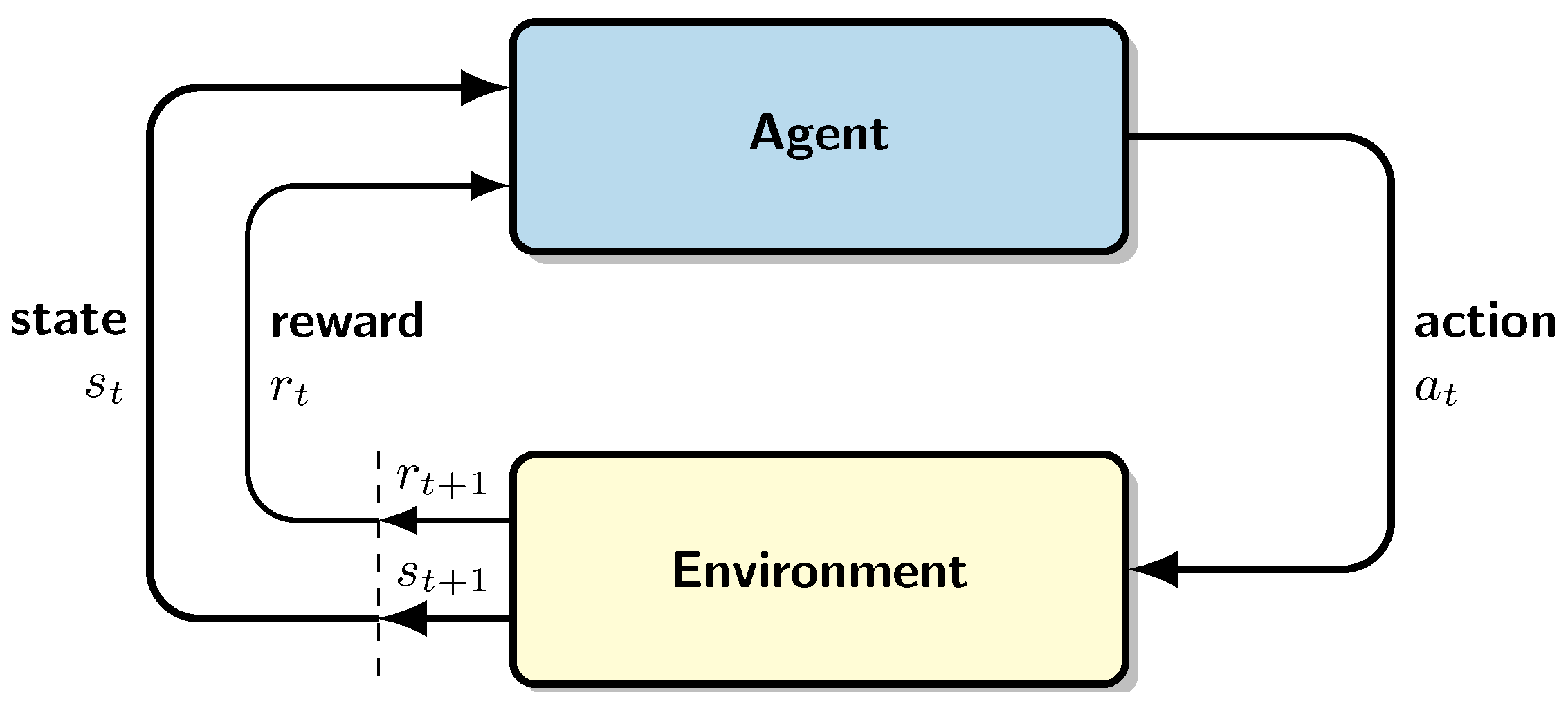
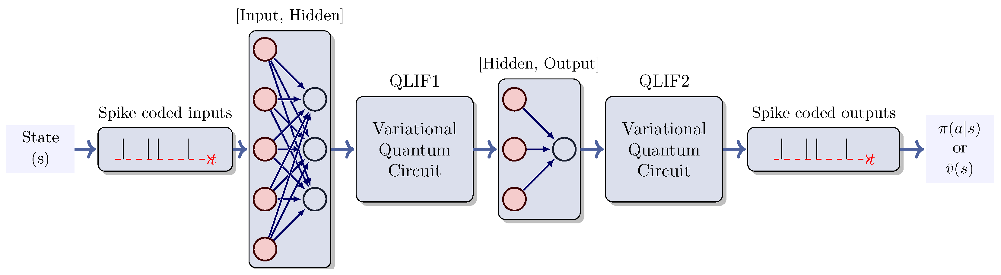
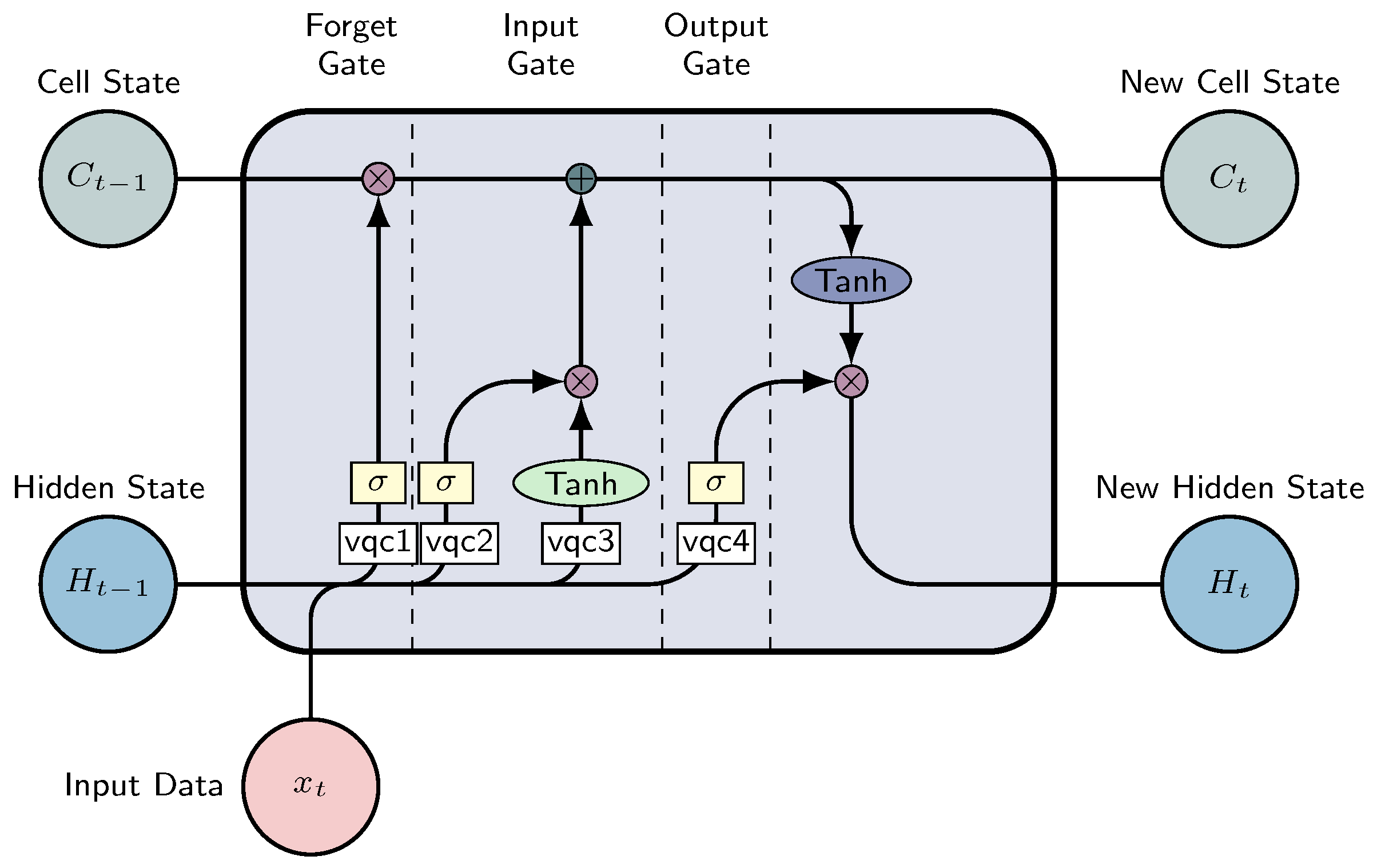
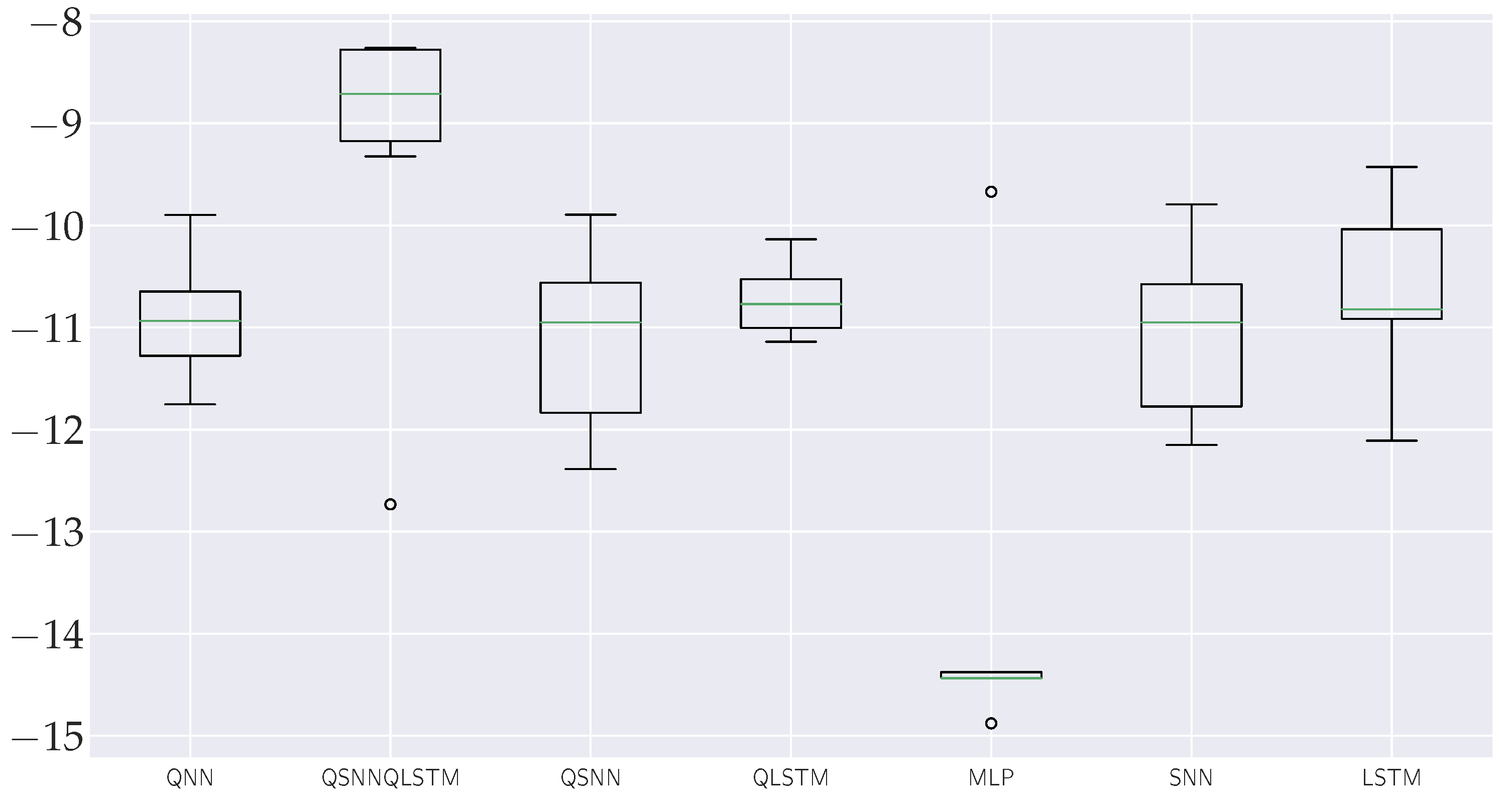
Table 1.
The observation variables consist of 14 variables, with an additional 3 empty variables reserved for specific problem requirements if necessary.
Table 1.
The observation variables consist of 14 variables, with an additional 3 empty variables reserved for specific problem requirements if necessary.
| Name | Units |
|---|---|
| Site-Outdoor-Air-DryBulb-Temperature | °C |
| Site-Outdoor-Air-Relative-Humidity | % |
| Site-Wind-Speed | m/s |
| Site-Wind-Direction | degree from north |
| Site-Diffuse-Solar-Radiation-Rate-per-Area | W/m2 |
| Site-Direct-Solar-Radiation-Rate-per-Area | W/m2 |
| Zone-Thermostat-Heating-Setpoint-Temperature | °C |
| Zone-Thermostat-Cooling-Setpoint-Temperature | °C |
| Zone-Air-Temperature | °C |
| Zone-Air-Relative-Humidity | % |
| Zone-People-Occupant-Count | count |
| Environmental-Impact-Total-CO2-Emissions-Carbon-Equivalent-Mass | Kg |
| Facility-Total-HVAC-Electricity-Demand-Rate | W |
| Total-Electricity-HVAC | W |
Table 2.
Action variables.
| Name | Heating Target Temperature | Cooling Target Temperature |
|---|---|---|
| 0 | 13 | 37 |
| 1 | 14 | 34 |
| 2 | 15 | 32 |
| 3 | 16 | 30 |
| 4 | 17 | 30 |
| 5 | 18 | 30 |
| 6 | 19 | 27 |
| 7 | 20 | 26 |
| 8 | 21 | 25 |
| 9 | 21 | 24 |
Table 3.
Configuration of classical models. Hyperparameters and settings for the artificial neural network, spiking neural network, and long short-term memory models, respectively.
Table 3.
Configuration of classical models. Hyperparameters and settings for the artificial neural network, spiking neural network, and long short-term memory models, respectively.
| MLP | SNN | LSTM | |
|---|---|---|---|
| Optimizer | Adam(lr = ) | Adam(lr = ) | Adam(lr = ) |
| Batch Size | 32 | 16 | 32 |
| BetaEntropy | 0.01 | 0.01 | 0.01 |
| Discount Factor | 0.98 | 0.98 | 0.98 |
| Steps | - | 15 | - |
| Hidden | - | 15 | 25 |
| Layers | Actor: [Linear[17, 450], ReLU | Actor: [Linear[17, 15] | Actor: [LSTM(17, 25, layers = 5) |
| Linear[450, 10]] | Lif1, Lif2 | Linear[25, 10]] | |
| Linear[15, 10]] | |||
| Critic: [Linear[17, 450], ReLU | Critic: [Linear[17, 15] | ||
| Linear[450, 1]] | Lif1, Lif2 | Critic: [LSTM(17, 25, layers = 5) | |
| Linear[15, 1]] | Linear[25, 1]] |
Table 4.
Configuration of quantum models. Hyperparameters and settings for the quantum neural network, quantum spiking neural network, quantum long short-term memory, and the novel model composed of the combination of the last two networks.
Table 4.
Configuration of quantum models. Hyperparameters and settings for the quantum neural network, quantum spiking neural network, quantum long short-term memory, and the novel model composed of the combination of the last two networks.
| QNN | QSNN | QLSTM | QSNN–QLSTM | |
|---|---|---|---|---|
| Optimizer | Adam(lr=) | Adam(lr = ) | Adam(lr = ) | [(Adam(QSNN.parameters, lr = ), |
| Adam(QLSTM.parameters, lr = ))] | ||||
| Batch Size | 128 | 16 | 128 | 128 |
| Pre-processing | Normalization | Normalization | - | Normalization |
| Post-processing | - | - | - | - |
| BetaEntropy | 0.01 | 0.01 | 0.01 | 0.01 |
| Discount Factor | 0.98 | 0.98 | 0.98 | 0.98 |
| Steps | - | 15 | 15 | 15 |
| Hidden | - | 15 | 25 | 15 (QSNN), 125 (QLSTM) |
| Layers | Actor: [[5 QNN] | Actor: [Linear[17, 15] | Actor: [Linear[17, 42] | |
| ReLU | 15 QSNN | Linear[42, 5] | ||
| Linear[, 10]] | Linear[15, 10]] | 4 VQCs | ||
| Linear[25, 5] | ||||
| Linear[5, 25] | ||||
| Linear[25, 10]] | ||||
| Critic: [[5 QNN | Critic: [Linear[17, 15] | Critic: [Linear[17, 42] | 5 QSNN | |
| ReLU | 15 QSNN | Linear[42, 5] | 5 QLSTM | |
| Linear[, 1]] | Linear[15, 1]] | 4 VQC’S | ||
| Linear[25, 5] | ||||
| Linear[5, 25] | ||||
| Linear[25, 1]] | ||||
| Qubits | 5 | 5 | 5 | 5 |
| Encoding Strategy | Amplitude Encoding | Amplitude Encoding | Angle Encoding | Amplitude Encoding |
Table 5.
Results obtained by classical and quantum models. Column 1: classical models followed by quantum versions and the novel quantum model proposed; Column 2: average total reward post-training; Column 3: best total reward post-training; Column 4: worst total reward post-training; Column 5: total reward (evaluation with deterministic policy); Column 6: computational time in seconds.
| Average Tot.Reward | Best Tot.Reward | Worst Tot.Reward | Test Reward | Time (s) | |
|---|---|---|---|---|---|
| MLP | −13.75 | −9.67 | −14.88 | −13.25 | 297.8 |
| SNN | −11.05 | −9.79 | −12.15 | −13.31 | 307.6 |
| LSTM | −10.56 | −9.43 | −12.11 | −12.67 | 302.8 |
| QNN | −10.92 | −9.90 | −11.75 | −12.87 | 326.1 |
| QSNN | −11.12 | −9.89 | −12.39 | −13.32 | 467.4 |
| QLSTM | −10.72 | −10.14 | −11.14 | −12.19 | 335.42 |
| QSNN–QLSTM | −9.40 | −8.26 | −12.73 | −11.83 | 962.5 |
Disclaimer/Publisher’s Note: The statements, opinions and data contained in all publications are solely those of the individual author(s) and contributor(s) and not of MDPI and/or the editor(s). MDPI and/or the editor(s) disclaim responsibility for any injury to people or property resulting from any ideas, methods, instructions or products referred to in the content. |
© 2024 by the authors. Licensee MDPI, Basel, Switzerland. This article is an open access article distributed under the terms and conditions of the Creative Commons Attribution (CC BY) license (https://creativecommons.org/licenses/by/4.0/).
Share and Cite
MDPI and ACS Style
Andrés, E.; Cuéllar, M.P.; Navarro, G. Brain-Inspired Agents for Quantum Reinforcement Learning. Mathematics 2024, 12, 1230. https://doi.org/10.3390/math12081230
AMA Style
Andrés E, Cuéllar MP, Navarro G. Brain-Inspired Agents for Quantum Reinforcement Learning. Mathematics. 2024; 12(8):1230. https://doi.org/10.3390/math12081230
Chicago/Turabian StyleAndrés, Eva, Manuel Pegalajar Cuéllar, and Gabriel Navarro. 2024. "Brain-Inspired Agents for Quantum Reinforcement Learning" Mathematics 12, no. 8: 1230. https://doi.org/10.3390/math12081230
Note that from the first issue of 2016, this journal uses article numbers instead of page numbers. See further details here.