
RUL Prediction for Piezoelectric Vibration Sensors Based on Digital-Twin and LSTM Network

1
School of Energy and Power Engineering, Beihang University, Beijing 100191, China
2
School of Reliability and Systems Engineering, Beihang University, Beijing 100191, China
*
Author to whom correspondence should be addressed.
Mathematics 2024, 12(8), 1229; https://doi.org/10.3390/math12081229
Submission received: 22 March 2024
/
Revised: 15 April 2024
/
Accepted: 18 April 2024
/
Published: 19 April 2024
(This article belongs to the Special Issue Mathematical Modelling and Computational Methods in Reliability Engineering)
Abstract
:Piezoelectric vibration sensors (PVSs) are widely used in high-temperature environments, such as vibration measurements in aero-engines, because of their high accuracy, small size, and high temperature resistance. Accurate prediction of its RUL (Remaining Useful Life) is essential for applying and maintaining PVSs. Based on PVSs’ characteristics and main failure modes, this work combines the Digital-Twin (DT) and Long Short-Term Memory (LSTM) networks to predict the RUL of PVSs. In this framework, DT can provide rich data collection, analysis, and simulation capabilities, which have advantages in RUL prediction, and LSTM network has good results in predicting time sequence data. The proposed method exploits the advantages of those techniques in feature data collection, sample optimization, and RUL multiclassification. To verify the prediction of this method, a DT platform is established to conduct PVS degradation tests, which generates sample datasets, then the LSTM network is trained and validated. It has been proved that prediction accuracy is more than 99.7%, and training time is within 94 s. Based on this network, the RUL of PVSs is predicted using different test samples. The results show that the method performed well in prediction accuracy, sample data utilization, and compatibility.
1. Introduction
With the development of aviation technology, intelligent propulsion system design and operation rely on the accuracy measurement of data from various sensors [1,2]. Vibration sensors can help monitor the vibration state of aero-engines and detect signs of malfunctions at an early stage [3]. For reliable monitoring, the sensors must be highly sensitive, low-quality, have a high signal-to-noise ratio, and be located as close to the high temperature and vibration source as possible [4]. Under these requirements, a piezoelectric vibration sensor (PVS) is exciting because of its high sensitivity, no need for an external power supply, and high temperature resistance [4,5,6]. For example, the CFM56 turbofan engine in the Boeing 737 uses PVSs to identify working states in every rotational cycle [7].
Since PVSs are widely used in aero-engine condition monitoring, it is significant to improve their reliability [8,9]. Despite advances in optimizing their materials and structure, the risk of PVS failure due to the effect of thermo-mechanical coupling, restricted to aero-engine working conditions, still exists [5,10]. As a result, remaining useful life (RUL) prediction is proposed to identify the state of PVS [11]. RUL prediction methods are generally divided into failure mechanism analysis, data-driven, and fusion [12,13,14]. The failure mechanism analysis method is established individually according to specific equipment. With the increasing complexity of equipment, the failure mechanism is generally too complex to obtain, or the cost is too high. The degradation of PVS under high temperatures involves a variety of mechanisms, which is still a limited topic [15]. Data-driven methods do not require the product specific knowledge such as material properties, constructions, and failure mechanisms. It can capture the complex relationships and learn trends available in the data without particular failure modes [16]. The fusion method refers to the combination of failure mechanism analysis and a data-driven model. Although it can fully use the advantages of the two methods, the process is relatively complex [16]. Therefore, research focuses on the data-driven RUL prediction method, which can be divided into statistical model-based and Machine Learning (ML)- based methods.
Our previous study used a statistical model-based data-driven approach and Digital-Twin (DT) to predict the RUL of PVS [17]. But there are still some problems. Firstly, a statistics-based data-driven approach must target well-defined degradation processes and ignore other failure modes. PVSs have failure modes like bias, gain, drifting, complete failure, noise, and constant with noise [18]. Secondly, the study is based on some assumptions: the degradation process of sensitivity conforms to the Wiener process, and the acceleration effect of temperature on the degradation process conforms to the Arrhenius formula. At the same time, the sensitivity of PVS needs to be measured indirectly using a calibration-like method. The sensitivity value of a VPS can only be obtained by analyzing its output and a standard vibration sensor under the same standard vibration condition. There will be errors in the filtering algorithm and signal synchronization. In addition, this measurement process limits the online measurement of PVS, which must be calibrated in isolation from actual conditions. Table 1 shows the different characteristics of different RUL prediction methods.
The data-driven approach based on ML can avoid the above problems. It establishes ML models by learning from past experimental data and existing knowledge for prediction [19]. ML-based methods achieved satisfactory results in RUL prediction, including support vector regression model (SVR) [20], multi-layer perceptron (MLP) [21], convolutional neural network (CNN) [22,23], recurrent neural network (RNN) [24,25], etc. In terms of input, the ML-based method can take the original output data and state information of PVS as input, preventing the error from the sensitivity calculation process and ignoring the assumptions in the statistical data-driven method. In terms of output, it not only skips the prediction of sensitivity degradation and predicts the RUL directly, but it also skips the selection of different failure modes. At the same time, the method can contain the data collected under various working conditions. Long Short-Term Memory (LSTM) is a network structure developed from Recurrent Neural Networks (RNN) to process time series data. As RNN have gradient vanishing/explosion problems when dealing with long-time dependence problems, LSTM’s memory cells and gating mechanisms are designed to solve this problem. In recent years, due to its adaptive classification of historical data to distinguish long-term memory data from short-term memory data, the LSTM network has been well applied in RUL prediction [26].
To capture the degradation data of PVS conveniently, DT provides a powerful tool for developing RUL prediction methods. Based on real-time interactions of DT between virtual models and physical structures, the degradation of a target system can be derived and evaluated effectively. DT is a way to organize and conduct RUL prediction bridges, and many studies show the efforts of DT frameworks applied in RUL prediction [27,28]. DT has favorable applications in RUL prediction involving vibration signals, such as rolling bearings [29,30] and other rotating machinery [31]. There are studies combining the advantages of DT and LSTM in RUL prediction [32,33,34,35].
In this paper, we use DT for data acquisition, processing, and simulation to obtain feature data and utilize the advantages of the LSTM network in RUL prediction for PVS. Table 2 shows the necessity of choosing DT and LSTM.
This work proposes a PVS-specific DT method and LSTM network for the task of RUL prediction. Our process seeks to predict the RUL in a novel way by using data from both working and testing conditions. The contributions of this work are threefold and summarized as follows:
- The PVS DT framework for RUL prediction based on the LSTM network is optimized and validated by building a DT platform for RUL prediction that fully utilizes the features of PVSs and sample datasets for the multiple failure modes. The scheme paves the way for DT and LSTM-based modeling of similar devices.
- A novel method to predict the RUL of PVS based on DT data and the LSTM network is proposed and provides accurate RUL prediction results for the PVS. It can help deal with degradation sequences with complex feature distribution and utilize the historical degradation data from different failure modes and non-failed samples.
- The influence of sample set parameters on the prediction effect is discussed through the training and validation of different training sets, verifying the method’s advantages in utilizing degraded data and prediction effect.
The general structure of this paper is organized as shown in Figure 1: In Section 2, previous studies on PVSs and their failure modes are reviewed as the basis of feather sections. In Section 3, we explain the DT architecture and relative factors of PVS RUL, which complete the DT platform and LSTM network needs. In Section 4, we explain the proposed method. In Section 5, we evaluate the proposed method and discuss the results, and finally, in Section 6, we conclude and suggest future work.
2. Structure and Failure Modes of PVS
2.1. Structure and Signal Characters of PVS
Generally, the PVS can be categorized into a shear type and a compression type, respectively, subjected to shear and compressive stress [36]. Figure 2 shows the structure of both types, which consist of similar components but have distinguishing mechanical characteristics. For both types, a PVS comprises a housing, a base, a connector, two mass blocks, a preload screw-pair, two piezoelectric elements, two conducting strips, and an insulating strip. The preload screw compacts the mass block, the piezoelectric elements, and the conducting strips together to form the preload structure. Notably, the preload direction of the compression-type PVS is consistent with the sensitive direction, while that of the shear type is vertical to the sensitive direction.
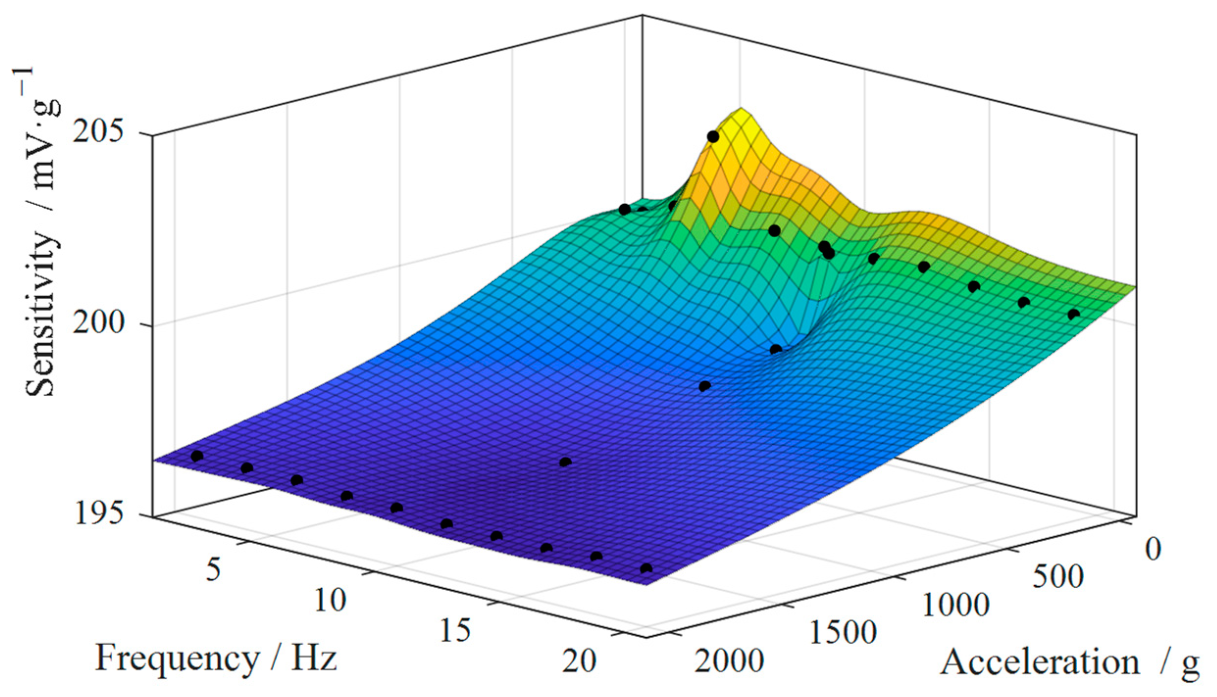
The preload structure converts the vibration of the base into a change in pressure on the piezoelectric element. Then, the piezoelectric effect converts the change of pressure into a change of charge. After that, a charge amplifier is needed to convert the charge signal output from the PVS into a voltage signal. In the high-temperature environment of aero-engines, the different materials of the preload structure have different temperature change characteristics, leading to changes in the preload force. The forces on the piezoelectric elements also vary under vibration of various frequencies and accelerations. These force variations affect the creep degradation of the material in the preloaded structure. At the same time, phenomena such as phase transition degradation and cracking of the piezoelectric elements under pressure and temperature stress lead to degradation of the piezoelectric coefficients. The rate of degradation is affected by temperature [15]. These conditions combine to cause the performance degradation of PVSs. This also leads to the sensitivity of PVS being inconsistent under the vibration conditions of different accelerations and frequencies. Figure 3 shows the distribution of sensitivity s with acceleration a and vibration frequency f for a particular model of PVS when calibrated at the factory.
As can be seen from the figure, there is an error in the sensitivity obtained if the sensitivity measurements are used directly without considering the vibration conditions. In the calibration of PVSs, a specific vibration condition (such as 160 Hz 10 g) is generally selected. However, under actual operating conditions, the vibration is not fixed, affecting the accuracy of sensitivity measurement. At the same time, the charge signal output from the PVS has to be filtered and converted to a voltage signal by a charge amplifier, which is then captured by the data acquisition (DAQ) card. These links also bring errors in the accurate measurement of PVSs.
2.2. Failure Analysis of PVS
PVSs are non-tightly connected electronic components with complex structures. This paper presents three typical shear PVS Failure Analysis (FA) cases: output short circuit, output open circuit, and sensitivity out-of-tolerance. The basic failure mechanisms are of those modes discussed in the following.
2.2.1. Output Short Circuit Caused by Coating Metal Whiskers Growth
Failure background: A PVS has no output after 240 h at 250 °C.
FA process: The appearance of the failed PVS is normal. The electrical parameters test finds that the output resistance is 120 Ω. The failure mode is output short-circuit. After the housing was disassembled, it was found that there were flocs between the piezoelectric element and the mass block through microscope observation. After further disassembling, it is observed that the flocs between the piezoelectric element and the mass block have the possibility of bonding the positive and negative poles, as shown in Figure 4.
After sampling and analysis by EDS (Energy Dispersive Spectrometer), it was determined that the flocs on the surface of the piezoelectric element are mainly silver and tungsten whiskers. By comparing the materials in each part of PVSs, it was confirmed that the silver element comes from the silver coating on the surface of the piezoelectric element, and tungsten came from the mass block. No other problems were found in inspecting the failed PVS, and parameter testing and disassembling analysis of the contrast parts did not find similar flocculent lapping.
FA conclusion: The failure is caused by the growth of metal whiskers in the silver coating from the piezoelectric element and tungsten from the mass block, which leads to the lap of the positive and negative poles and the short circuit of the sensor output.
2.2.2. Output Open Circuit Caused by Solder Joint Fracture
Failure background: A PVS has no output after 1400 h at 220 °C.
FA process: No abnormality was found during the appearance check of the failure sensor. An output open was found in the electrical parameter test. And the X-ray examination showed no exception. After unsealing, it was found that the solder joint of the lead and the conducting strip was abnormal. The connection was broken, and the solder had an obvious melting trace, as shown in Figure 5. Direct measurement of both ends of the solder joint found that it was a break. Both ends of the solder joint and the sensor’s output leads were measured, and no break was seen. The output impedance was standard after lapping the lead and the conducting strip. No other anomalies were found after further disassembly.
FA conclusion: The reason for PVS failure is that the solder joints of the wire and conducting strip soften and break under high temperature and vibration, leading to an output open circuit.
2.2.3. Sensitivity Out-of-Tolerance
Failure background: After working in a high-temperature environment for hundreds of hours, the sensitivity of several PVS is out of tolerance and drops beyond the qualified threshold.
FA process: The appearance inspection was regular, the sensitivity test was below the threshold, the output resistance was expected, and the X-ray examination was regular. No abnormality was found after the shell was disassembled; no exception was seen by the microscope examination of the internal structure after the disassembly, and the local resistance test was standard. After disassembling the internal parts, it was found that there were piezoelectric cracks in some sensors, as shown in Figure 6.
FA conclusion: After excluding other possible reasons, it is judged that the piezoelectric coefficient is reduced after the piezoelectric element’s failure or the preloaded structure’s change, which leads to a decrease in sensitivity and out-of-tolerance.
Based on the FA cases and daily use experience, the main failure modes of PVSs include output short-circuit, output open circuit, and sensitivity out-of-tolerance. Considering the applied stresses that meet the PVS design criteria, the most common failure mode is sensitivity degradation, leading to sensitivity out-of-tolerance. This occurs through degradation of the piezoelectric coefficient of the piezoelectric element itself, damage to the piezoelectric element, and failure of the preloaded structure until the sensitivity exceeds the failure threshold and the PVS fails.
3. DT-Based PVS RUL Analysis
3.1. DT Architecture for PVS RUL Prediction Based on LSTM Network
Typically, a five-dimensional DT model of PVS covers the physical entities, virtual entities, and connections between them, as well as the data and services, as shown in Figure 7, where represents the physical entity, VE is the virtual equipment, Ss indicates the services for PE and VE, DD refers to DT data, and CN is the connection, among other parts.
Aiming to predict the RUL of PVS by the LSTM network, an RUL prediction DT framework based on DT data and LSTM is established based on previous research [17]. As shown in Figure 8, the main improvement is in the content of the virtual model management and application module, which adjusts the content of each module from data acquisition to processing and application according to the needs of LSTM. On the one hand, this framework involves all five dimensions in the proposed PVS-specific DT model. On the other hand, the RUL prediction method has six basic modules that present the real-time PVS status, deal with both physical and virtual working conditions, and provide users with prediction results. Each module of the framework is described in detail below.
Application and test module: This module belongs to PE, and contain the PE setup for PVS working and testing and the VE application for calculating, simulation, and organization of data, and training, validation, and prediction of the LSTM network.
Virtual model management module: This module belongs to VE and refers to all models in VE. For LSTM-based prediction, features preprocessing methods, sample data organization methods, and LSTM network are added for sample generation and network training and prediction.
Virtual model application module: This module belongs to Ss and CN and is the bridge between VE and DD. For LSTM, the module adds data preprocessing, sample data organization, training, and validation functions for RUL prediction.
Data management module: This module belongs to DD and Ss and supports interactions among different modules. Considering the application of LSTM, it adds feature data, training dataset, validation dataset, and network training data.
Expandable module: This module belongs to Ss and is responsible for the expansion of PE devices, VE models, Ss protocols, and DD datasets. The method upgrade is also performed in this module.
Visualization module: This module belongs to Ss. The main additions are the training monitoring of LSTM network and the comparison of training data, including the convergence process of the network and the confusion matrix of validation results.
3.2. Relative Factors Analysis of RUL for PVS
RUL refers to the remaining useful life of a product after a period of use. RUL at time t is generally defined as follows:
where is the failure time. Predicting the RUL of a product requires a quantitative characterization of the degradation process. The degradation process of PVSs mainly manifests in the degradation of sensitivity [17], so sensitivity is a necessary feature. According to the analysis in Section 2.1, the sensitivity varies according to the vibration frequency and acceleration, which should be considered. At the same time, the degradation rate is also affected by the temperature, the time under temperature, and the pressure of piezoelectric elements. The selected features include sensitivity s, frequency f, acceleration a, temperature T, time t, and pressure P, as shown in Table 3.
Among them, time and temperature can be obtained directly. The sensitivity, vibration frequency, and acceleration need to be acquired from the output of PVS and analyzed using the signal processing model in DT. The pressure of the piezoelectric element needs to be obtained by the finite element simulation module in DT. Figure 9 shows how feature data are obtained from the DT.
3.2.1. Calculation of Features in DT
Figure 10 shows the calculation method for sensitivity s. The vibration signal is applied to both the PVS to be tested and the standard one to ensure that both PVSs are under the same vibration conditions. Then, the sensor output charge signal was converted to a voltage signal after charge amplifier and band-pass filtering and then acquired by the DAQ card.
The test PVS and standard PVS measure the same vibration signal, so their output of the vibration acceleration peak and frequency is the same. According to this, it can be obtained as follows
which can be transformed to the following:
where known sensitivity of standard PVS, and are known parameters of charge amplifiers, while and can be measured during testing. The sensitivity of the test PVS is thus determined. Accordingly, by analyzing the output of the standard PVS, the frequency f and peak acceleration a under the current vibration condition can be obtained. The data set measured under different vibration conditions can achieve an accurate description of the sensitivity.
3.2.2. Simulation of Features in DT
The pressure of the piezoelectric elements mainly depends on the pretension of the preload structure. Still, it also varies with temperature due to the different coefficients of thermal expansion of the materials in each part. The pressure of the piezoelectric elements under various conditions can be obtained by a finite element simulation model in DT, which depends on the design data and material parameters. Figure 11 shows the pressure distribution of piezoelectric elements in a PVS with a typical parallel structure.
After steps of direct measurement, data analysis, and finite element simulation in DT, the degradation feature data of PVS with different samples, time, and vibration states can be obtained, which are merged to form the degradation feature dataset and the corresponding RUL dataset , in which denotes the sensitivity distribution dataset for different vibration conditions.
4. RUL Prediction Algorithm Based on DT Data and LSTM Network
Modeling using historical degradation data and then model correction using real-time degradation data is a popular strategy in RUL prediction. In a previous study [17], sensitivity degradation is modeled, and the time at which the degradation first reached the failure threshold was predicted as a method of RUL prediction. This approach assumes that the time at which sensitivity degradation reaches a threshold is the time to failure. Failure modes other than sensitivity degradation tolerance are ignored. This is subject to some error. Also, this assumption ignores samples with different failure modes, resulting in the lack of utilization for historical degradation data. In addition, due to the sensitivity distribution originating from vibration frequency and acceleration, it is necessary to unify the measurement conditions when modeling the sensitivity degradation. This requires that the historical degradation data and the real-time degradation data of the test PVS are measured under the same vibration conditions, which is not conducive to applying the RUL prediction method. This paper proposes a method for PVS RUL prediction using DT data and the LSTM network to solve the above problems. The details of the algorithm are described next.
4.1. LSTM Structure Details
The LSTM network is a special kind of RNN, mainly used to solve the gradient vanishing and gradient explosion problems while training long sequences; thus, LSTM can work better in long sequences. LSTM has been widely used for RUL prediction because it is suitable for time series prediction [37,38,39]. The primary cell structure of the LSTM network is shown in Figure 12, which effectively controls the consequences caused by accumulation by introducing cell states, forgetting gates, input gates, and output gates.
Based on the currently given input x and the hidden layer output h from the previous moment, the LSTM network update process is shown as follows [38,40]:
By constantly repeating the choice of forgetting or remembering, the LSTM network realizes the selection of sequence data and avoids the gradient explosion problem of RNN.
4.2. Data Organization
PVS is costly and not used often, so the stock of historical degradation data is limited. To generate sufficient neural network training samples with fewer PVSs, the amount of data at an individual time needs to be increased, and the degradation sequences need to be expanded. To improve the training of the LSTM network, it is necessary to convert the numerical prediction of RUL into a classification prediction of RUL intervals and to balance the number of samples for each classification.
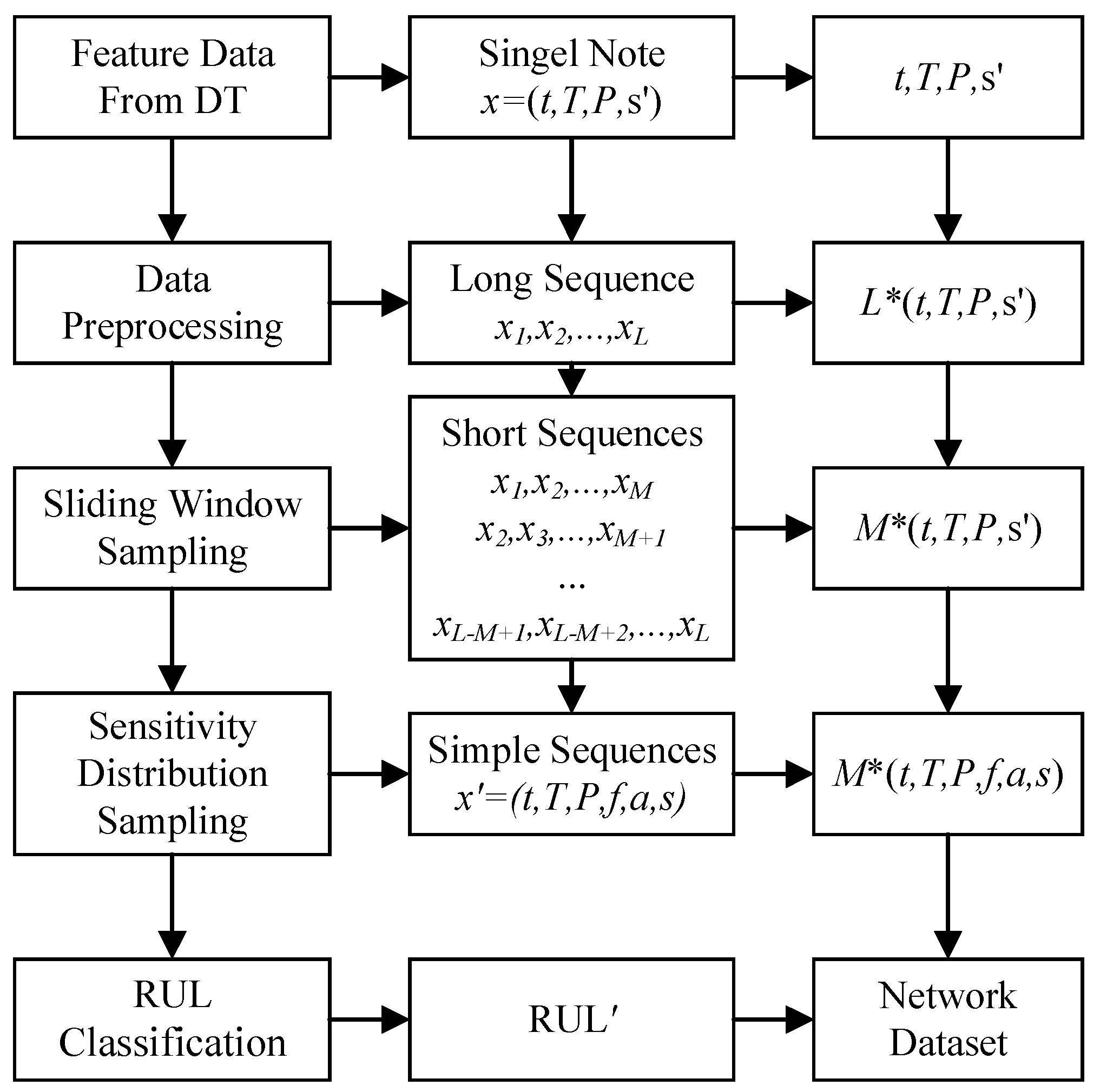
The flow of data organization is shown in Figure 13. The basic requirements for the distribution of in the feature dataset provided by DT are first determined. We use x to represent the basic data in single node. Then, a long sequence of degradation feature data from a single PVS is sampled by a sliding window with fixed size M to obtain short sequences , ,…, . The distribution of sensitivity with vibration conditions is sampled multiple times to obtain , which realizes sample amplification. After that, the RUL of the last time of each short sequence is classified to obtain the classification dataset . This converts the regression problem of RUL prediction into a classification problem to provide utilization of historical data and prediction accuracy. In this way, the samples required for the training and validation of the LSTM network are obtained.
These data organization efforts are in the process of degradation features data collection, individual sample generation, and training sample set generation, respectively.
4.2.1. Degradation Features Data Collection
During the degradation data acquisition process of the PVSs, DT records the outputs and related background information and obtains the degradation data set and RUL data set . From the analysis in Section 2.1, it is known that is data set that describes the distribution of sensitivity under different vibration conditions. For samples used for neural network training, the coverage of the distribution by the sample data needs to be considered. Taking the research object of this paper, a shear PVS, as an example, referring to its typical working conditions, the vibration conditions are selected as shown in Table 4, which cover low frequency, high frequency, and different acceleration values. Let the number of condition groups be N. The acquired under these vibrational conditions allows for a better characterization of the sensitivity distribution. In this way, the specific measurement conditions and ensemble size of in the degradation dataset are clarified.
4.2.2. Sample Optimization Based on Sliding Window and Sensitivity Distribution Data Sampling
The degradation data for each PVS have different sequence sizes due to different failure times and measurement times, while the training samples have data size consistency requirements. The sliding window method is often used in LSTM network to sample long sequences into a series of short sequences of fixed size, increasing the number of training samples and unifying the sample size. The sliding window process is shown in Figure 14.
For long degradation data sequence of a single PVS with a size of L:
where is a single element in the degradation data set. The long sequence can be sampled with a sliding window of size M to obtain short sequences, which are as follows:
A complex sample structure will cause a decrease in network learning speed and prediction accuracy. At the same time, since the input data of neural network prediction should be consistent with the form of training samples, the complexity of the sample structure can also make it challenging to obtain input data for prediction. Specifically, for a short sequence of the form , the inputs need to include sensitivity distributions at M points, each consisting of N sets of . The size of a single sample data exceeds . The method in this paper samples the data sets of sensitivity distributions at each time in the short sequence to generate simpler sample sequences. This ensures the sample set carries information about the sensitivity distributions by sampling multiple times. The method procedure is shown in Figure 15. For every node in the short sequence , a set of is randomly sampled from the sensitivity distribution dataset . These are merged with other data in the same nodes to form a simplified short sequence sample , where . Such sampling is repeated n times to amplify the original short sequence with a complex form into n samples of simplified structure . The network trained with such samples has better compatibility in prediction by requiring only sensitivity values for a single vibration condition.
Eventually, for each PVS degradation sample, the number of samples generated from the long sequence through sliding window sampling and sensitivity distribution data sampling can be up to . Generally, the longer the short sequence, the more information there is in a single sample, and the total number of samples decreases, but it also results in a more significant amount of data needed for the initial prediction. The more sampling times there are, the more complete the sample information coverage is and the better the prediction effect is. However, too many samples will also bring about an increase in training time.
4.2.3. Classification of RUL
For each short sequence sample , the RUL value of the last node is used as the corresponding sample output. RUL prediction for PVS is performed to replace them before failure and prevent losses caused by failure. The work to be performed is the same for PVSs with RULs that are less than the replacement threshold. The accuracy of regression prediction for RUL brings limited significance. Meanwhile, regression prediction has requirements on the coverage effect of the training samples. On the other hand, acquiring RUL values relies on the regular testing of PVS in the degradation test. Failure time is often detected later than the actual time of failure. These result in systematic errors in the measured RUL, centrally distributed over regular monitoring intervals. In summary, it is more appropriate to use classification prediction in training sample set generation. The interval with the largest RUL value in the classification is often in the form of , which can also realize the full utilization of partially degradation data of unfailed PVS. As long as the PVS has not failed time after a specific time, the RUL at that time can be classified as the maximum interval. When setting the RUL classification intervals, it is necessary to consider the actual demand of RUL prediction and balance the number of samples for each classification. Finally, the sample classification dataset is obtained.
4.3. Network Training and Performance Evaluation
Before training the LSTM network, the dataset must be divided into a training and a validation set. Specifically, 70% of the dataset is used for training and 30% for testing. The output of the LSTM network is passed through a Softmax function to get the probability distribution of the output classification. Then, the results are compared with the data labels to get the cross entropy, thus obtaining the Cross-Entropy Loss (CEL). Equations (7) and (8) show the Softmax and cross-entropy functions [41,42]:
where n is the number of RUL types and is the output (predicted value) of the ith network unit.
where N is the number of training samples, is the tactual classification of sample i, and is the network’s predicted value for sample i.
To evaluate the model’s performance, the classification accuracy, the ratio of correctly classified validation samples to the total number of validation samples, was used as the evaluation metric, and the model’s accuracy on the test set was recorded as the final performance metric.
5. Results and Discussion
5.1. Degradation Data Acquisition
A verification platform was established to validate the RUL prediction algorithm based on DT data and the LSTM network. Figure 16 shows a photograph of the test rig.
During this experiment, both a test PVS and a standard PVS were installed in a vibration exciter to observe degradation. Vibration signals undergo transformation via a charge amplifier and are detected utilizing a data acquisition (DAQ) card and a host computer. A power supply serves as the electrical source for the system, while a waveform generator provides a standard signal in the system. Moreover, a high-temperature test chamber is employed to replicate thermal stress conditions. Detailed specifications for each piece of equipment are provided in Table 5.
Ten PVSs are randomly selected from the same batch and named as (A1, A2), (B1, B2), (C1, C2), (D1, D2), and (E1, E2), respectively. To ascertain the efficacy of our approach, the individual variability between the two samples within the same group is considered negligible. The test procedures for all groups are outlined as follows:
- All samples are placed in the high-temperature test chamber and subjected to heating at a constant rate;
- After the determined heating time, the samples are removed from the test chamber with a fixed cooling rate and installed on the vibration exciter;
- The vibration condition is set at 28 typical conditions as listed in Table 2, and the function and sensitivity of the PVSs are recorded;
- The test is terminated once a PVS sample fails.
The temperature settings vary for each PVS group, as detailed in Table 6.
The experimental results of different PVSs are shown in Table 7. Failure modes include output short circuit, open circuit, and sensitivity out-of-tolerance. Some PVSs recorded up to 3000 h without failure. It can be seen that the lifetime of the PVSs increases as the test temperature decreases. However, there are still more unusual individuals among them, which illustrates the complexity of the sample distribution.
5.2. LSTM Network Training and Validation
5.2.1. DT Data Pre-Processing and Organization
Each feature value is extracted and analyzed for the degradation test data collected in the DT platform. Time t and temperature T can be obtained directly from the test conditions and state data. The piezoelectric element pressure P can be obtained through the thermal simulation function of the virtual model application module in DT. Through the sensor output processing function of the virtual model application module in DT, the actual vibration condition frequency f, acceleration a, and sensitivity s can be obtained through the workflow in Figure 9 and Figure 10. On this basis, the degradation data set of PVSs is obtained.
A sliding window is applied to the long-time sequence of each PVS sample to obtain short sequences of fixed size. The sequence sizes M were taken from 5 to 20 to generate different sample sets to compare the prediction effect of the network. Considering that the demand of sample size can be satisfied when arranging combinations of vibration conditions at various times in the short sequences, 1000 combinations can be randomly selected to improve the training speed. The final sample sets are obtained, as shown in Table 8. It can be seen that the number of samples obtained by the sliding window decreases as the size of the sequence increases.
The RUL corresponding to each short sequence is calculated from the time of the last node in the sequence by Equation (1). Based on the actual demand for RUL prediction and the distribution of test data, the classification of the RUL prediction task for this model PVS was finally set to the range shown in Table 9. With this classification range, the classification of each RUL value can be determined, obtaining the dataset . The data set of those samples that experienced 3000 h without failure can be utilized for their 0–1800 h degradation data and the RUL categorized in the last class.
The computer used for the experiments is equipped with an AMD EPYC 7642 CPU, 4 NVIDIA GeForce RTX4090 GPUs, and 256 G RAM. Model training was carried out using the Adam optimizer in PyTorch, based on the Tsai framework from GitHub repositories [43]. Specifically, 20 epochs were trained with a batch size 1024 and a learning rate 0.001.
5.2.2. Comparison of Different Sequence Sizes
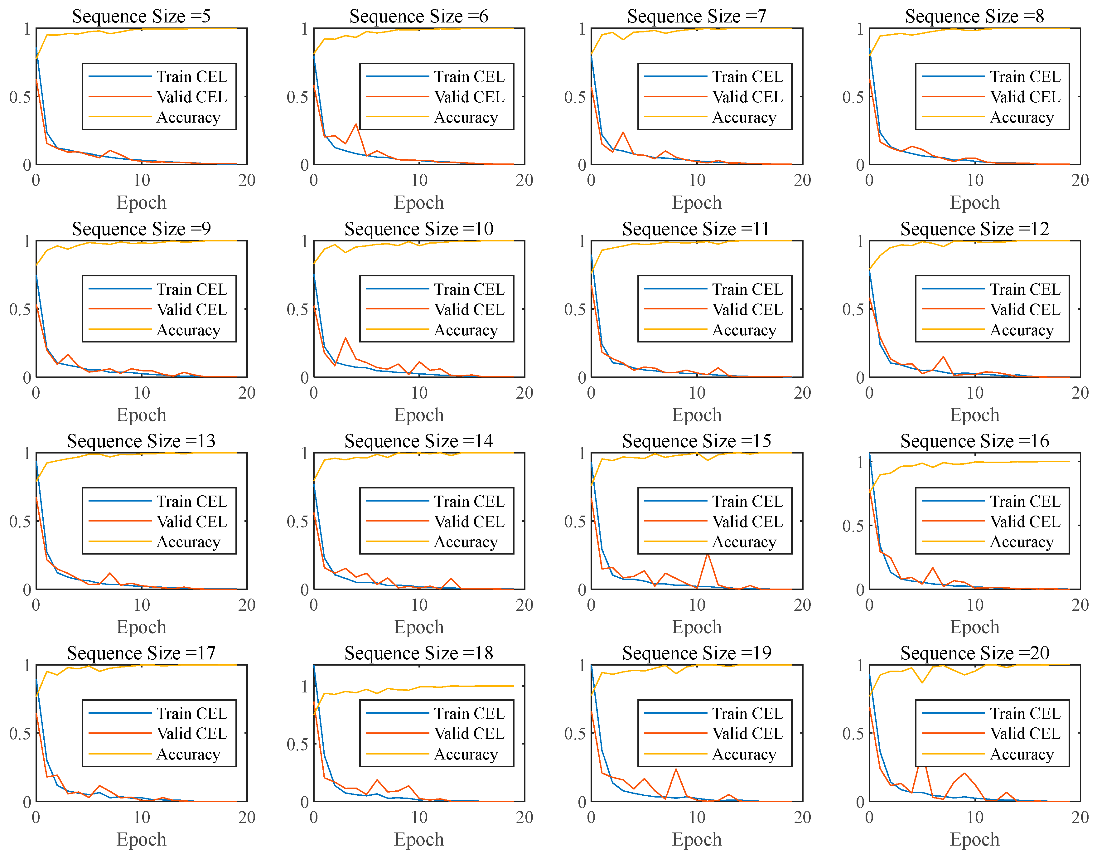
Figure 17 shows the changes in CEL and accuracy for training sets with different sequence sizes. Under each sequence size, the CEL of the training and validation sets decreases, the training accuracy improves, and the network training effect improves.
The variation in the number of samples and training time for different sequence sizes is shown in Figure 18. It can be seen that when the sequence size is increased from 5 to 20, the size of samples is almost halved, and the training time is reduced from 94.0 to 48.4 s. This shows that for a fixed original long sequence, an increase in the size of the sample sequence leads to a decrease in the size of training samples and network training time. The specific data are shown in Table 8 and Table 10.
The CEL and validation accuracy of the last epoch at different sequence sizes are shown in Figure 19. It can be seen that as the sequence size increases from 5 to 20, the CEL in the training and validation sets decreases by several times, and the validation accuracy keeps improving from 99.79% to 99.99%. It can be seen that for a fixed original long sequence, an increase in the size of the sample sequence brings about an improvement in the prediction. The specific data are shown in Table 8 and Table 10.
Analyzing the network prediction details, the confusion matrix for the worst predicted sequence size 5, for example, is shown in Figure 20. We can see that the distribution of test samples is good, and the vast majority of test samples can be classified correctly, proving the model’s training effect and the method’s prediction effect.
5.2.3. Comparison of Different Sensitivity Sampling Sizes
To compare the effect of sensitivity data sampling size on the network, the datasets are generated by sampling from 50 to 5000 times at the two extremes of sequence size 5 and 20, respectively. The networks are trained with these datasets separately, provided that the rest of the parameters are kept consistent. The number of samples and training time for different sensitivity sampling numbers are shown in Figure 21. As can be seen from it, sample size and training times continue to increase with increasing sensitivity sampling size, both for sequence sizes 5 and 20.
The final epoch’s CEL and accuracy of different sensitivity sampling sizes are shown in Figure 22. Whether the sequence size is 5 or 20, as the sensitivity sampling size increases, the CEL of the final epoch decreases significantly, and the accuracy keeps improving. This demonstrates that the increase in the sensitivity sampling size helps the samples better characterize the sensitivity distribution and improves the accuracy of LSTM prediction.
In particular, a sensitivity sampling size of 1000 is big enough for a good prediction. Suppose we increase the sensitivity sampling size further. In that case, the prediction accuracy will be of limited benefit, and the training complexity and time will continue to grow, so the current parameter setting of 1000 sensitivity sampling is reasonable enough.
5.3. RUL Prediction Case Based on DT and LSTM
Based on the above methodology, RUL prediction for PVS was carried out using DT. A new PVS sample F of the same model was selected to operate at a temperature of 473.15 K. After collecting and preprocessing its output and other features using the DT platform, the LSTM network trained with the historical data was used to predict the RUL of sample F until it failed to confirm the true RUL.
5.3.1. RUL Prediction Based on Single Sample
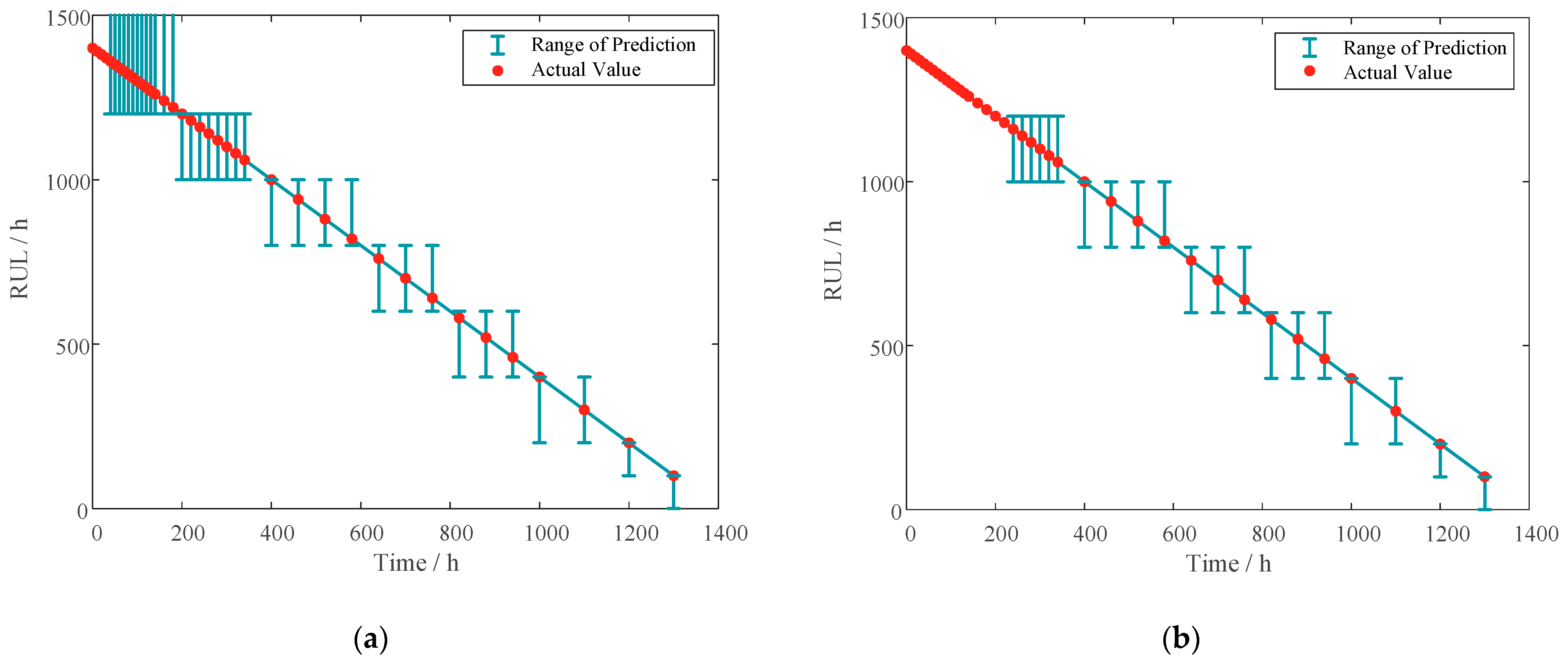
According to the discussion in Section 4.2, the present LSTM network can predict simple degenerate sequence samples with single-point vibration conditions. To verify the network’s prediction ability for a single sample, the data processing of sample F starts with one sensitivity degradation sampling for each time node to obtain a long sequence with only one set of data . Two sets of samples are obtained using sliding window sampling with sequence sizes of 5 and 20, respectively. The trained LSTM network predicts these samples; the results are shown in Figure 23. It can be seen that the actual RUL is within the prediction range since the prediction starts, and the method is validated for its ability to predict single samples. Meanwhile, by comparing the difference between the prediction starting points in the two results, the initial prediction can be realized earlier using the LSTM network with short sequence sizes.
Combined with the analysis in Section 4.3, the choice of the feature sequence size affects not only the network training time and prediction accuracy but also the time to obtain the RUL prediction value for the first time. Hence, it needs to be chosen according to the actual needs.
5.3.2. RUL Prediction Based on Multi-Samples from Sensitivity Sampling
To fully utilize the degradation data of sample F, more prediction samples are generated for prediction through sensitivity data sampling. In the degradation data preprocessing, the sensitivity distribution is sampled 1000 times to create the prediction sample set of sequence size 5. The dataset is imported into the trained LSTM network for prediction. The prediction range for each time node and its prediction probability are shown in Figure 24. As can be seen in the figure, the prediction probability gradually increases as time gets closer to failure, indicating that the network is becoming more and more confident.
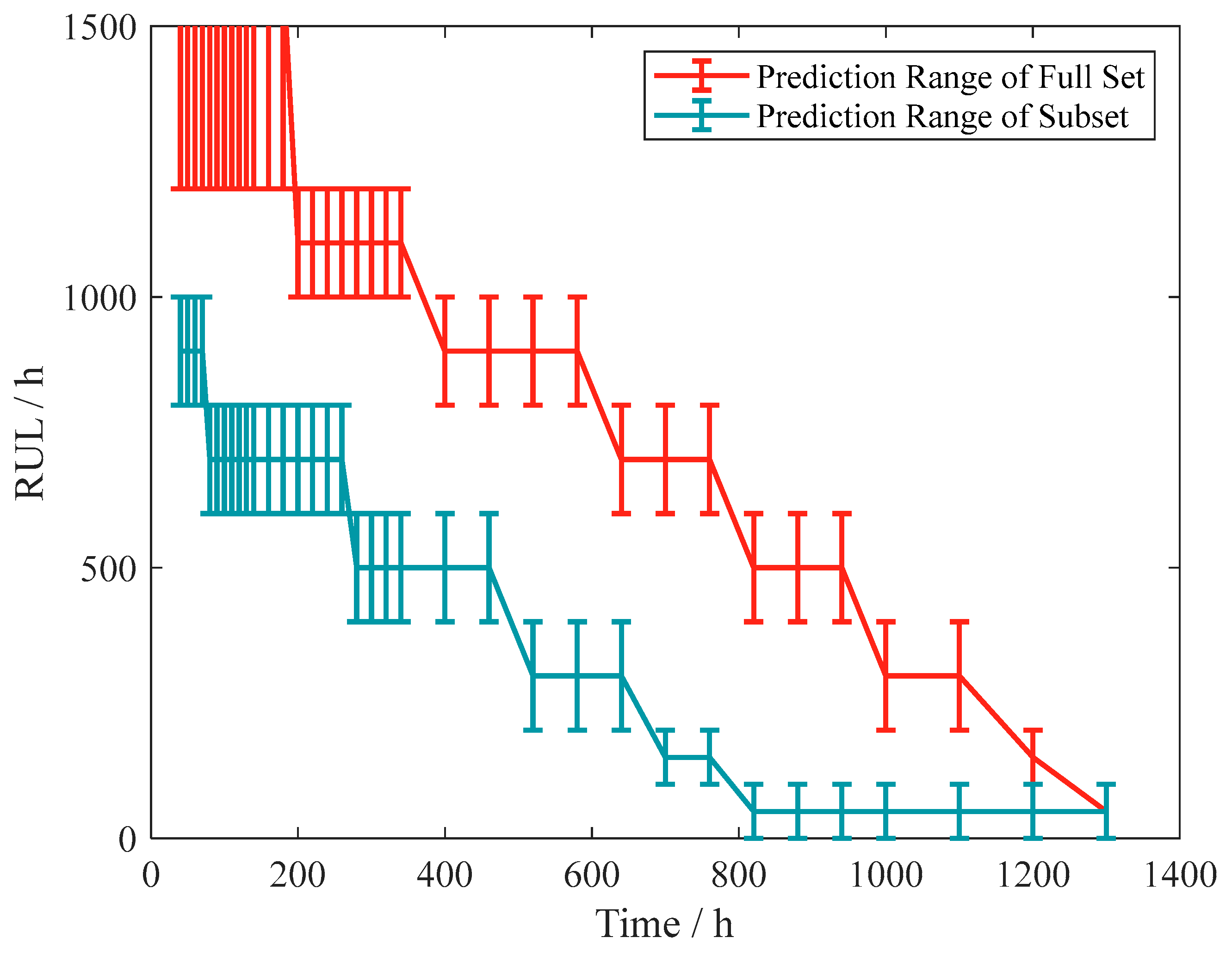
5.3.3. RUL Prediction Based on Samples from Single Failure Mode
As analyzed in Section 4, the LSTM method can fully use the historical degradation data from whose failure modes are not only sensitivity degradation out of tolerance. This gives a more comprehensive dataset and trains a better network. To compare the effect of data from different failure mode sources on network training, only data from samples A2, B2, and C2, whose failure modes are sensitivity degradation out-of-tolerance, were used to generate the training set and train the LSTM network. The RUL of sample F is predicted using the trained network, and the prediction results are shown in Figure 25.
As can be seen from the results, there is a clear difference between the results predicted by the full dataset (from multiple failure modes) and the subset (from a single failure mode). Analyzing the reason for this, it can be seen from Table 7 that the PVS samples whose failure mode is sensitivity degradation out-of-tolerance have an earlier failure time than the other samples. After the LSTM network has fully learned the characteristics of this sub-training set, it gives RUL predictions that tend to be more conservative. In the practical use of the algorithm, such a prediction tendency will lead to an earlier replacement of PVS, resulting in waste. Meanwhile, by comparing the prediction effect of the subset, the advantage of this method on the compatibility of historical degradation data with different failure modes is also verified.
6. Conclusions
This paper proposes a method for RUL prediction of PVS based on DT and LSTM networks. First, the structure and signal characteristics of the PVS were analyzed, and the main failure modes of the PVS were identified through FA. Then, the DT framework of PVS for RUL prediction was improved, and the factors related to RUL prediction were summarized. After that, an algorithm for RUL prediction based on DT data and the LSTM network was proposed. It includes feature value collection method, sample optimization method based on sliding window and sensitivity distribution sampling, and RUL classification method. The network training evaluation method was also analyzed. Finally, a DT platform was constructed to conduct degradation tests on PVS samples, and the degradation data were collected and analyzed by DT and trained by the LSTM network. The trained network is used to predict the RUL of the degraded cases. The following conclusions can be drawn.
- The DT framework for PVS is optimized to meet the needs of LSTM-based prediction of RUL, which fully uses PVS features and sample datasets for multiple failure modes. It is verified by PVS degradation tests and training, validation, and prediction of the LSTM network. A method for the RUL prediction of PVS based on DT data and the LSTM network is proposed. It includes the degradation feature data collection method, a sample optimization method based on sliding window and sensitivity distribution data sampling, and a RUL classification and prediction approach. The effectiveness of the method is verified by the degradation test of PVS. Under the experimental real sample set and hardware conditions, the validation set prediction accuracy is above 99.7%, and the total training time is within 94 s.
- The influence of sample set parameters on the prediction effect is discussed through the training and validation of different training sets, including the sequence size, sensitivity sampling size, and failure mode coverage. When the sequence size is increased from 5 to 20, the size of samples is almost halved, the training time is reduced from 94.0 to 48.4 s, the CEL in the training and validation sets decreases by several times, and the validation accuracy keeps improving from 99.79% to 99.99%. As the sensitivity sampling size increases, the CEL of the final epoch decreases significantly, and the accuracy keeps improving. In particular, a sensitivity sampling size of 1000 is big enough for a good prediction.
- The compatibility of the method with different forms of sample and prediction demands is verified by comparing the prediction process for single and multiple samples. The effect of the data source on the prediction effect of the LSTM model was analyzed by comparing the prediction effect of the training set from different failure mode samples. This also validates the compatibility of the present method with different failure modes and partially unfailed degradation data. The proposed RUL prediction method can help deal with degradation sequences with complex feature distribution and utilize the historical degradation data from different failure modes and non-failed samples.
Author Contributions
Conceptualization, C.F.; Data curation, C.F.; Formal analysis, W.Z.; Funding acquisition, C.G.; Methodology, C.F.; Project administration, C.G.; Resources, C.G.; Software, C.F.; Supervision, C.G.; Validation, C.G. and W.Z.; Visualization, W.Z.; Writing—original draft, C.F.; Writing—review and editing, C.F. All authors have read and agreed to the published version of the manuscript.
Funding
This research was funded by the equipment research project in advance Grant No. 41402040301 and research fund NO.2021-0048/YZQT0003.
Data Availability Statement
The data are available from the authors upon request.
Acknowledgments
Thanks to C. Wang who gave support to the writing and F. Gao and F. Zhong who assisted with the experimental conditions. Thanks to the support from FON research group.
Conflicts of Interest
The authors declare no conflicts of interest.
References
- Koskoletos, A.O.; Aretakis, N.; Alexiou, A.; Romesis, C.; Mathioudakis, K. Evaluation of Aircraft Engine Gas Path Diagnostic Methods Through ProDiMES. J. Eng. Gas. Turbines Power-Trans. ASME 2018, 140, 12. [Google Scholar] [CrossRef]
- Hunter, G.W.; Wrbanek, J.D.; Okojie, R.S.; Neudeck, P.G.; Fralick, G.C.; Chen, L.Y.; Xu, J.; Beheim, G.M. Development and application of high temperature sensors and electronics for propulsion applications. In Proceedings of the Conference on Sensors for Propulsion Measurement Applications, Kissimmee, FL, USA, 20–21 April 2006. [Google Scholar]
- Kulagin, V.P.; Akimov, D.A.; Pavelyev, S.A.; Potapov, D.A. Automated Identification of Critical Malfunctions of Aircraft Engines Based on Modified Wavelet Transform and Deep Neural Network Clustering. In Proceedings of the Workshop on Materials and Engineering in Aeronautics (MEA), Moscow, Russia, 16–17 October 2019. [Google Scholar]
- Kim, K.; Zhang, S.J.; Salazar, G.; Jiang, X.N. Design, fabrication and characterization of high temperature piezoelectric vibration sensor using YCOB crystals. Sens. Actuator A-Phys. 2012, 178, 40–48. [Google Scholar] [CrossRef]
- Jiang, C.; Liu, X.L.; Yu, F.P.; Zhang, S.J.; Fang, H.R.; Cheng, X.F.; Zhao, X. High-temperature Vibration Sensor Based on Ba2TiSi2O8 Piezoelectric Crystal with Ultra-Stable Sensing Performance up to 650 °C. IEEE Trans. Ind. Electron. 2021, 68, 12850–12859. [Google Scholar] [CrossRef]
- Han, C.Y.; Zhao, C.Y.; Ding, H.; Chen, C. Temperature-insensitive polarimetric vibration sensor. Opt. Lett. 2022, 47, 2714–2717. [Google Scholar] [CrossRef] [PubMed]
- How Vibration Informs the Maintenance of Aircraft Engines. Available online: https://www.aerospacetestinginternational.com/features/how-vibration-data-informs-the-maintenance-of-aircraft-engines.html (accessed on 1 August 2023).
- Yuan, Y.; Liu, X.F.; Ding, S.T.; Pan, B.C. Fault Detection and Location System for Diagnosis of Multiple Faults in Aeroengines. IEEE Access 2017, 5, 17671–17677. [Google Scholar] [CrossRef]
- Trivedi, S.; Ganesh, R.H.; Shen, T.; Huang, P.W.; Li, S.S.; IEEE. Piezoelectric MEMS Vibration Sensor Module for Machining Quality Prediction. In Proceedings of the IEEE Sensors Conference, Rotterdam, The Netherlands, 25–28 October 2020. [Google Scholar]
- Wei, H.F.; Geng, W.P.; Bi, K.X.; Li, T.; Li, X.M.; Qiao, X.J.; Shi, Y.K.; Zhang, H.Y.; Zhao, C.Q.; Xue, G.; et al. High-Performance Piezoelectric-Type MEMS Vibration Sensor Based on LiNbO3 Single-Crystal Cantilever Beams. Micromachines 2022, 13, 329. [Google Scholar] [CrossRef] [PubMed]
- Liu, Y.; Sun, B.; IEEE. Remaining Useful Life Prediction of MEMS Sensors Used in Automotive Under Random Vibration Loading. In Proceedings of the 59th Annual Reliability and Maintainability Symposium (RAMS), Orlando, FL, USA, 28–31 January 2013. [Google Scholar]
- Wang, S.; Jin, S.; Bai, D.; Fan, Y.; Shi, H.; Fernandez, C. A critical review of improved deep learning methods for the remaining useful life prediction of lithium-ion batteries. Energy Rep. 2021, 7, 5562–5574. [Google Scholar] [CrossRef]
- Wang, X.; Ye, P.; Liu, S.; Zhu, Y.; Deng, Y.; Yuan, Y.; Ni, H. Research Progress of Battery Life Prediction Methods Based on Physical Model. Energies 2023, 16, 3858. [Google Scholar] [CrossRef]
- Lei, J.; Zhang, W.; Jiang, Z.; Gao, Z. A Review: Prediction Method for the Remaining Useful Life of the Mechanical System. J. Fail. Anal. Prev. 2022, 22, 2119–2137. [Google Scholar] [CrossRef]
- Salazar, R.; Serrano, M.; Abdelkefi, A. Fatigue in piezoelectric ceramic vibrational energy harvesting: A review. Appl. Energy 2020, 270, 115161. [Google Scholar] [CrossRef]
- Cheng, S.; Pecht, M.; IEEE. A Fusion Prognostics Method for Remaining Useful Life Prediction of Electronic Products. In Proceedings of the IEEE International Conference on Automation Science and Engineering, Bangalore, India, 22–25 August 2009; pp. 102–107. [Google Scholar]
- Fu, C.; Gao, C.; Zhang, W. A Digital-Twin Framework for Predicting the Remaining Useful Life of Piezoelectric Vibration Sensors with Sensitivity Degradation Modeling. Sensors 2023, 23, 8173. [Google Scholar] [CrossRef]
- Kullaa, J. Detection, identification, and quantification of sensor fault in a sensor network. Mech. Syst. Signal Proc. 2013, 40, 208–221. [Google Scholar] [CrossRef]
- Sawant, V.; Deshmukh, R.; Awati, C. Machine learning techniques for prediction of capacitance and remaining useful life of supercapacitors: A comprehensive review. J. Energy Chem. 2023, 77, 438–451. [Google Scholar] [CrossRef]
- Wang, X.-l.; Gu, H.; Xu, L.; Hu, C.; Guo, H. A SVR-Based Remaining Life Prediction for Rolling Element Bearings. J. Fail. Anal. Prev. 2015, 15, 548–554. [Google Scholar] [CrossRef]
- Tian, Z.G. An artificial neural network method for remaining useful life prediction of equipment subject to condition monitoring. J. Intell. Manuf. 2012, 23, 227–237. [Google Scholar] [CrossRef]
- Song, Y.; Gao, S.Y.; Li, Y.B.; Jia, L.; Li, Q.Q.; Pang, F.Z. Distributed Attention-Based Temporal Convolutional Network for Remaining Useful Life Prediction. IEEE Internet Things J. 2021, 8, 9594–9602. [Google Scholar] [CrossRef]
- Li, X.; Ding, Q.; Sun, J.Q. Remaining useful life estimation in prognostics using deep convolution neural networks. Reliab. Eng. Syst. Saf. 2018, 172, 1–11. [Google Scholar] [CrossRef]
- Zheng, S.; Ristovski, K.; Farahat, A.; Gupta, C.; IEEE. Long Short-Term Memory Network for Remaining Useful Life Estimation. In Proceedings of the IEEE International Conference on Prognostics and Health Management (ICPHM), Dallas, TX, USA, 19–21 January 2017; pp. 88–95. [Google Scholar]
- Liao, Y.; Zhang, L.X.; Liu, C.D.; IEEE. Uncertainty Prediction of Remaining Useful Life Using Long Short-Term Memory Network Based on Bootstrap Method. In Proceedings of the IEEE International Conference on Prognostics and Health Management (ICPHM), Seattle, WA, USA, 11–13 June 2018. [Google Scholar]
- Berghout, T.; Benbouzid, M. A Systematic Guide for Predicting Remaining Useful Life with Machine Learning. Electronics 2022, 11, 1125. [Google Scholar] [CrossRef]
- Ma, J.; Ma, S.; Zhang, H.; Li, R.; Xiao, P. Research on Modeling Method of Crack Propagation Life Prediction for Digital Twin Frame. Mach. Des. Res. 2023, 39, 172–177. [Google Scholar]
- Peng, A.; Ma, Y.; Huang, K.; Wang, L. Digital twin-driven framework for fatigue life prediction of welded structures considering residual stress. Int. J. Fatigue 2024, 181, 108144. [Google Scholar] [CrossRef]
- Zhao, W.; Zhang, C.; Fan, B.; Wang, J.; Gu, F.; Peyrano, O.G.; Wang, S.; Lv, D. Research on rolling bearing virtual-real fusion life prediction with digital twin. Mech. Syst. Signal Proc. 2023, 198, 110434. [Google Scholar] [CrossRef]
- Meng, W.; Wang, Y.; Zhang, X.; Li, S.; Bai, X.; Hou, L. Prediction of fault evolution and remaining useful life for rolling bearings with spalling fatigue using digital twin technology. Appl. Intell. 2023, 53, 28611–28626. [Google Scholar] [CrossRef]
- Zhang, C.; Ma, Z.; Liu, B.; Sun, Z.; Xu, J. Digital Twin Driven Few-Shot Prediction of Remaining Useful Life for Rotating Machinery. J. Xi’an Jiaotong Univ. 2023, 57, 168–178. [Google Scholar]
- Zhao, W.; Zhang, C.; Wang, J.; Wang, S.; Lv, D.; Qin, F. Research on Digital Twin Driven Rolling Bearing Model-Data Fusion Life Prediction Method. IEEE Access 2023, 11, 48611–48627. [Google Scholar] [CrossRef]
- Cheng, X.; Lv, K.; Zhang, Y.; Wang, L.; Zhao, W.; Liu, G.; Qiu, J. RUL Prediction Method for Electrical Connectors with Intermittent Faults Based on an Attention-LSTM Model. IEEE Trans. Compon. Packag. Manuf. Technol. 2023, 13, 628–637. [Google Scholar] [CrossRef]
- Lyu, G.; Zhang, H.; Miao, Q. Parallel State Fusion LSTM-based Early-cycle Stage Lithium-ion Battery RUL Prediction Under Lebesgue Sampling Framework. Reliab. Eng. Syst. Saf. 2023, 236, 109315. [Google Scholar] [CrossRef]
- Wang, Z.; Liu, N.; Chen, C.; Guo, Y. Adaptive self-attention LSTM for RUL prediction of lithium-ion batteries. Inf. Sci. 2023, 635, 398–413. [Google Scholar] [CrossRef]
- Wu, G.d.; Liu, X.l.; Yu, F.p.; Li, F.l.; Tian, S.w.; Cheng, X.f.; Zhao, X. The Accelerometer Utilizing the Transverse Vibration Mode of LGT Piezoelectric Crystal. In Proceedings of the 13th Symposium on Piezoelectrcity, Acoustic Waves and Device Applications (SPAWDA), Harbin, China, 11–14 January 2019; pp. 1–5. [Google Scholar]
- Chen, X. A novel gear RUL prediction method by diffusion model generation health index and attention guided multi-hierarchy LSTM. Sci. Rep. 2024, 14, 1795. [Google Scholar] [CrossRef] [PubMed]
- Guo, R.; Li, H.; Huang, C. Operation stage division and RUL prediction of bearings based on 1DCNN-ON-LSTM. Meas. Sci. Technol. 2024, 35, 025035. [Google Scholar] [CrossRef]
- Yao, X.; Zhu, J.; Jiang, Q.; Yao, Q.; Shen, Y.; Zhu, Q. RUL prediction method for rolling bearing using convolutional denoising autoencoder and bidirectional LSTM. Meas. Sci. Technol. 2024, 35, 035111. [Google Scholar] [CrossRef]
- Yu, Y.; Hu, C.; Si, X.; Zheng, J.; Zhang, J. Averaged Bi-LSTM networks for RUL prognostics with non-life-cycle labeled dataset. Neurocomputing 2020, 402, 134–147. [Google Scholar] [CrossRef]
- Xu, J.; Liu, B.; Zhou, Y.; Liu, M.; Yao, R.; Shao, Z. Diverse Image Captioning via Conditional Variational Autoencoder and Dual Contrastive Learning. ACM Trans. Multimed. Comput. Commun. Appl. 2024, 20, 1–16. [Google Scholar] [CrossRef]
- Yang, X.W.; Zhang, A.X.; Zhao, C.R.; Yang, H.X.; Dou, M.F. Categorization of ECG signals based on the dense recurrent network. Signal Image Video Process. 2024, 18, 3373–3381. [Google Scholar] [CrossRef]
- Ignacio, O. tsai—A State-of-the-Art Deep Learning Library for Time Series and Sequential Data. Available online: https://github.com/timeseriesAI/tsai (accessed on 9 October 2023).
Figure 1.
Paper structure.

Figure 2.
The main structure types of PVSs: (a) shear-type PVS; (b) compression-type PVS.

Figure 3.
Distribution of sensitivity of typical PVS with vibration conditions.

Figure 4.
Flocs between the piezoelectric plate and mass block.

Figure 5.
Solder joints of lead and the conductive plates of the failed PVS.

Figure 6.
Cracks on the piezoelectric elements of multiple PVSs with out-of-sensitivity.

Figure 7.
The architecture of the PVS five-dimension DT model.

Figure 8.
The architecture of a DT for RUL prediction.

Figure 9.
RUL-related features of PVS.

Figure 10.
PVS sensitivity analysis process.

Figure 11.
Pressure distribution of a PVS.

Figure 12.
LSTM network basic cell structure.

Figure 13.
LSTM-based RUL prediction method for PVS.

Figure 14.
Sliding window sampling process.

Figure 15.
Sampling process for sensitivity distributions.

Figure 16.
Experimental platform.

Figure 17.
CEL and accuracy changes during training.

Figure 18.
Sample size and training time for different sequence sizes.

Figure 19.
CEL and accuracy for different sequence sizes.

Figure 20.
Confusion matrix of predicted results.

Figure 21.
Sample size and training time for different sensitivity sampling sizes: (a) sequence size 5; (b) sequence size 20.
Figure 21.
Sample size and training time for different sensitivity sampling sizes: (a) sequence size 5; (b) sequence size 20.

Figure 22.
CEL and accuracy for different sensitivity sampling sizes: (a) sequence size 5; (b) sequence size 20.
Figure 22.
CEL and accuracy for different sensitivity sampling sizes: (a) sequence size 5; (b) sequence size 20.

Figure 23.
PVS RUL classification prediction results: (a) sequence size 5; (b) sequence size 20.

Figure 24.
RUL prediction results of sample F are based on multiple samples.

Figure 25.
Prediction result of LSTM trained by different datasets.


Table 1.
Comparison of RUL prediction methods.
| RUL Prediction Method | Failure Mechanism | Data-Driven | Fusion Method | |
|---|---|---|---|---|
| Statistical Model-Based | ML-Based | |||
| Characteristic | insight | clear distribution range | massive calculation | complex |
| Failure mode | specific | specific | most | undetermined |
| Sample quantity | few | few | more | undetermined |
| For PVS | failure mechanism not clear | only for sensitivity degradation | insufficient training data set | undetermined |
| Conclusion | difficult | operable | operable | more difficult |
Table 2.
Comparison of DT and LSTM network in RUL prediction.
| RUL Prediction Based on | LSTM | DT and Degradation Modeling (Previous Paper) | DT and LSTM (This Paper) |
|---|---|---|---|
| Failure mode | no need | single | no need |
| other need | sequence data | degradation data characteristics | Sensitivity distribution acquisition |
| Computation amount | large | small | large |
| Sample size | large | small | sensitivity distribution sampling to increase |
| Suitable object | Li battery, ball bearing, complex equipment, but no studies for PVS | PVS, depends on the degradation data distribution characteristics | PVS, devices with complex feature distribution |
Table 3.
Feature of PVS RUL prediction.
| Feature | Variable | Unit |
|---|---|---|
| Time | t | h |
| Temperature | T | K |
| Pressure | P | N |
| Frequency of vibration | f | Hz |
| Acceleration of vibration | a | m·s−2 |
| Sensitivity | s | pC m−1·s2 |
Table 4.
Vibration conditions of degradation data acquisition.
| NO. | f/Hz | a/g | NO. | f/Hz | a/g | NO. | f/Hz | a/g |
|---|---|---|---|---|---|---|---|---|
| 1 | 100 | 2 | 11 | 2000 | 2 | 21 | 20 | 10 |
| 2 | 100 | 4 | 12 | 2000 | 4 | 22 | 40 | 10 |
| 3 | 100 | 6 | 13 | 2000 | 6 | 23 | 80 | 10 |
| 4 | 100 | 8 | 14 | 2000 | 8 | 24 | 160 | 10 |
| 5 | 100 | 10 | 15 | 2000 | 10 | 25 | 315 | 10 |
| 6 | 100 | 12 | 16 | 2000 | 12 | 26 | 630 | 10 |
| 7 | 100 | 14 | 17 | 2000 | 14 | 27 | 1250 | 10 |
| 8 | 100 | 16 | 18 | 2000 | 16 | 28 | 2000 | 10 |
| 9 | 100 | 18 | 19 | 2000 | 18 | |||
| 10 | 100 | 20 | 20 | 2000 | 20 |
Table 5.
Test equipment specifications.
| Device | Parameters |
|---|---|
| High-temperature test chamber | LIGAO HF-100FN, 300 K~600 K |
| Vibration exciter | SINOCERA JZK-20, 200 N, 30 g |
| Power supply | SINOCERA YE5874, 810 W |
| Waveform generator | KEYSIGHT 33500B, 30 MHz, 5 V |
| Standard VPS | Endevco 6222S-20A, 200 mV/g |
| Charge amplifier | Endevco 2777A-10-10, 10 Hz~10 kHz |
| Host computer | ThinkStation P350, Intel i7 11700 |
| DAQ card | NI Compact DAQ 9232, 3 channel, 102.4 kS/s/ch |
Table 6.
Test temperature.
| PVS Number | Temperature/K |
|---|---|
| A1 and A2 | 523.15 |
| B1 and B2 | 493.15 |
| C1 and C2 | 473.15 |
| D1 and D2 | 448.15 |
| E1 and E2 | 423.15 |
Table 7.
Experimental results.
| PVS Number | Failure Time/h | Failure Modes |
|---|---|---|
| A1 | 240 | output short circuit |
| A2 | 600 | sensitivity out-of-tolerance |
| B1 | 1400 | output open circuit |
| B2 | 880 | sensitivity out-of-tolerance |
| C1 | >3000 | - |
| C2 | 1400 | sensitivity out-of-tolerance |
| D1 | >3000 | - |
| D2 | 200 | output open circuit |
| E1 | >3000 | - |
| E2 | >3000 | - |
Table 8.
Number of samples with different sequence sizes.
| Sequence Size | Samples | Training Samples | Testing Samples |
|---|---|---|---|
| 5 | 289,000 | 202,300 | 86,700 |
| 6 | 279,000 | 195,300 | 83,700 |
| 7 | 269,000 | 188,300 | 80,700 |
| 8 | 260,000 | 182,000 | 78,000 |
| 9 | 251,000 | 175,700 | 75,300 |
| 10 | 242,000 | 169,400 | 72,600 |
| 11 | 233,000 | 163,100 | 69,900 |
| 12 | 224,000 | 156,800 | 67,200 |
| 13 | 215,000 | 150,500 | 64,500 |
| 14 | 206,000 | 144,200 | 61,800 |
| 15 | 197,000 | 137,900 | 59,100 |
| 16 | 188,000 | 131,600 | 56,400 |
| 17 | 179,000 | 125,300 | 53,700 |
| 18 | 170,000 | 119,000 | 51,000 |
| 19 | 162,000 | 113,400 | 48,600 |
| 20 | 154,000 | 107,800 | 46,200 |
Table 9.
RUL classification range.
| Classification | 1 | 2 | 3 | 4 | 5 | 6 | 7 | 8 |
|---|---|---|---|---|---|---|---|---|
| RUL Range/h | (0, 100] | (100, 200] | (200, 400] | (400, 600] | (600, 800] | (800, 1000] | (1000, 1200] | (1200, +∞) |
Table 10.
Prediction accuracy and training time for different sequence sizes.
| Sequence Size | Training Time/s | Train CEL | Valid CEL | Accuracy/% |
|---|---|---|---|---|
| 5 | 93.95805931 | 0.004598 | 0.006693 | 99.786 |
| 6 | 87.52612972 | 0.003087 | 0.004678 | 99.857 |
| 7 | 85.31973052 | 0.002984 | 0.004185 | 99.887 |
| 8 | 84.82289147 | 0.002089 | 0.003432 | 99.905 |
| 9 | 78.97516322 | 0.00206 | 0.002597 | 99.938 |
| 10 | 73.74387383 | 0.002939 | 0.002127 | 99.964 |
| 11 | 73.66227794 | 0.00157 | 0.001924 | 99.961 |
| 12 | 70.45144176 | 0.00189 | 0.001249 | 99.978 |
| 13 | 67.65879798 | 0.001438 | 0.001075 | 99.980 |
| 14 | 66.34648776 | 0.001964 | 0.000739 | 99.985 |
| 15 | 58.13756585 | 0.000953 | 0.000787 | 99.983 |
| 16 | 60.89499235 | 0.001465 | 0.00081 | 99.991 |
| 17 | 59.87257957 | 0.001182 | 0.000621 | 99.989 |
| 18 | 57.55060816 | 0.001325 | 0.000511 | 99.996 |
| 19 | 55.03493381 | 0.001172 | 0.000498 | 99.996 |
| 20 | 48.43837452 | 0.00144 | 0.000709 | 99.994 |
Disclaimer/Publisher’s Note: The statements, opinions and data contained in all publications are solely those of the individual author(s) and contributor(s) and not of MDPI and/or the editor(s). MDPI and/or the editor(s) disclaim responsibility for any injury to people or property resulting from any ideas, methods, instructions or products referred to in the content. |
© 2024 by the authors. Licensee MDPI, Basel, Switzerland. This article is an open access article distributed under the terms and conditions of the Creative Commons Attribution (CC BY) license (https://creativecommons.org/licenses/by/4.0/).
Share and Cite
MDPI and ACS Style
Fu, C.; Gao, C.; Zhang, W. RUL Prediction for Piezoelectric Vibration Sensors Based on Digital-Twin and LSTM Network. Mathematics 2024, 12, 1229. https://doi.org/10.3390/math12081229
AMA Style
Fu C, Gao C, Zhang W. RUL Prediction for Piezoelectric Vibration Sensors Based on Digital-Twin and LSTM Network. Mathematics. 2024; 12(8):1229. https://doi.org/10.3390/math12081229
Chicago/Turabian StyleFu, Chengcheng, Cheng Gao, and Weifang Zhang. 2024. "RUL Prediction for Piezoelectric Vibration Sensors Based on Digital-Twin and LSTM Network" Mathematics 12, no. 8: 1229. https://doi.org/10.3390/math12081229
Note that from the first issue of 2016, this journal uses article numbers instead of page numbers. See further details here.