

A Sustainable Supply Chain Model with Low Carbon Emissions for Deteriorating Imperfect-Quality Items under Learning Fuzzy Theory


Department of Statistics, University of Tabuk, Tabuk 71491, Saudi Arabia
*
Author to whom correspondence should be addressed.
Mathematics 2024, 12(8), 1237; https://doi.org/10.3390/math12081237
Submission received: 16 March 2024
/
Revised: 11 April 2024
/
Accepted: 14 April 2024
/
Published: 19 April 2024
(This article belongs to the Special Issue Advances and Application of Fuzzy Sets, Decision Making and Soft Computing)
Abstract
:In this paper, we develop a two-level supply chain model with low carbon emissions for defective deteriorating items under learning in fuzzy environment by using the double inspection process. Carbon emissions are a major issue for the environment and human life when they come from many sources like different kinds of factories, firms, and industries. The burning of diesel and petrol during the supply of items through transportation is also responsible for carbon emissions. When any company, firm, or industry supplies their items through a supply chain by using of transportation in the regular mode, then a lot of carbon units are emitted from the burning of petrol and diesel, etc., which affects the supply chain. Carbon emissions can be controlled by using different kinds of policies issued by the government of a country, and lots of companies have implemented these policies to control carbon emissions. When a seller delivers a demanded lot size to the buyer, as per demand, and the lot size has some defective items, as per consideration, the demand rate is uncertain in nature. The buyer inspects the received whole lot and divides it into two categories of defective and no defective deteriorating items, as well as immediately selling at different price. The fuzzy concept nullifies the uncertain nature of the demand rate. This paper covers two models, assuming two conditions of quality screening under learning in fuzzy environment: (i) the buyer shows the quality screening and (ii) the quality inspection becomes the seller’s responsibility. The carbon footprint from the transporting and warehousing the deteriorating items is also assumed. The aim of this study is to minimize the whole inventory cost for supply chains with respect to lot size and the number of orders per production cycle. Jointly optimizing the delivery lot size and number of orders per production cycle will minimize the whole fuzzy inventory cost for the supply chain and also reduce the carbon emissions. We take two numerical approaches with authentic data (from the literature reviews) for the justification of the proposed model 1 and model 2. Sensitivity observations, managerial insights, applications of these proposed models, and future scope are also included in this paper, which is more beneficial for firms, the industrial sector, and especially for online markets. The impact of the most effective parameters, like learning effect, fuzzy parameter, carbon emissions parameter, and inventory cost are shown in this study and had a positive effect on the total inventory cost for the supply chain.
Keywords:
double screening process; learning fuzzy theory; supply chain; carbon emissions; transportation; deteriorating imperfect itemsMSC:
90B061. Introduction
Nowadays, many production industries produce a large of number of items for more profit using supply chain processes, and during the production of items, transportation of items, or burning of petrol and diesel by these causes, a lot of carbon units exit in the form of carbon emissions, which damages the ware housing of greening items, environment, and human lifestyle. Supply chain management (SCM)is a good tool for the coordination of customers, buyers, and sellers and also exerts a favorable effect on stock replenishment decisions. Supply chains are also more beneficial for quality improvement, the supply of inventory material, and inventory decision cost information. Carbon emissions affect the supply chain directly or indirectly and cannot be ignored in the supply chain. If the demand for the item is constant or deterministic, then the supply chain runs smoothly and the producer or seller obtains more profit, but on the other hand, if demand for the items is uncertain, then the producer or seller obtains unexpected profit or unexpected loss, and obtaining no profit or no loss may be dependent on that situation. Hence, the analysis of the demand rate of items cannot ignored during the supply of items. During the production of items, each produced item should be good in quality, but this is not generally true, because in the produced lot, some items may not be good due to some technical problems. In this proposed model, it is considered that each lot has some defective items. The seller delivers then demanded lot of deteriorating perfect-quality items to the buyer and the buyer separates the received lot from the seller through an inspection process and divides the whole lot into two categories, where one is good-quality items and other is poor-quality items. The buyer sells both types of items at different prices and also assumes the effect of deterioration. The present scenario incorporates learning concepts, a lock fuzzy environment, carbon emissions, and economic order quantity in this supply chain. We consider that each lot of production has some defective items. With this concept in mind, we develop a supply chain inventory model with low carbon emissions for imperfect deteriorating items under a learning and lock fuzzy environment and present a scenario also assuming the effect of deterioration during the supply chain. The present scenario examines the effect of deterioration, learning, parameters of the lock fuzzy environment, and different types of cost parameters on the joint inventory cost during the supply chain. For the development of the proposed study, we describe a literature review regarding this study in the literature review section.
1.1. Literature Study Based on EOQ, Carbon Emissions, and Supply Chain Management (SCM)
This section covers the basic literature study that helps in the development of this proposed study. In this order, the supply chain is the backbone of the inventory theory because it connects the seller, buyer, and customer, and the manager can observe to see the supply chain and remove unnecessary factors from the supply chain, which affects the selling of items. Glock [1] explained the many problems regarding EOQ through an inventory model and also found an expression for the lot size. Many authors have developed EOQ inventory models with different approaches under carbon emissions. In this order, Luo et al. [2] developed a supply chain inventory model with inventory policies under low carbon emissions for various items and also showed the effect of low carbon emissions, and Das et al. [3] presented new collection of literature reviews of supply chains under carbon emissions and compared old results with recent results of different supply chain inventory models, as well as gave new approach for the supply chain. Kazmi et al. [4] generalized an EOQ model with trade credit policy for imperfect-quality items under carbon emissions and also explained the effect of a trade credit period on the buyer’s profit and seller’s profit. From the motivation of Kazmi et al. [4], Sarkar et al. [5] presented a sustainable supply chain model (SCM) with multiple trade credit policies for the effect of environment issues under a partial backlogging case, and suggested a lot of managerial insights for the investors of shareholders. Taleizadeh et al. [6] suggested an EPQ model with shortages for the production system under carbon emissions and examined the effect of shortages on the EPQ system. Sarkar et al. [7] developed a three-echelon supply chain system with transportation under the impact of carbon emissions and showed the effect of variable transportation on the supply chain, as well as showing the impact of carbon emissions on the joint profit of the supply chain. Sarkar et al. [8] improved the model of Sarkar et al. [7] with the help of multiple trade credit policies for the global sustainable supply chain model under the impact of carbon emissions. Daryanto et al. [9], motivated by the work of Sarkar et al. [8], improved the inventory model with the impact of carbon emissions for deteriorating items under two-level supply chain management. Wahab et al. [10] developed the work of Daryanto et al. [9] by using the international supply chain model for imperfect-quality items and environment issues. In this view, Jauhari et al. [11] improved the fantastic work of Wahab et al. [10] by using unequal lot size policy and carbon emissions under a two-level supply chain model for imperfect-quality items and cooperative policy. Sarkar et al. [12] considered a game theory approach with carbon emissions in the supply chain model under a reduction in ordering cost. Jauhari et al. [13] assumed a stochastic-demand-based supply chain model for imperfect-quality items under carbon emissions and the variations in stochastic demand when changing inventory parameters were also explained deeply. Gautam and Khanna [14] explained a production-based inventory model with carbon emissions under an inspection process and also presented the policy of ordering cost reduction by using of the carbon emissions policy, as well as calculating the joint total profit the supply chain. Tiwari et al. [15] developed a carbon-emissions-based supply chain model for deteriorating imperfect-quality items under an inspection process and showed the effect of deterioration on the joint profit during the supply chain.
1.2. Literature Study Regarding Imperfect-Quality-Based Inventory Model
In general, we see that in many industries, production companies are trying to produce good items, but in reality, this is not true, and they also produce a fixed percentage of defective-quality items. Many authors have worked on the imperfect production system one, like Rosenblatt and Lee [16], who gave a basic inventory model for imperfect-quality item sunder production processes and explained managerial insights for new researchers or investors of shareholders or inspectors of the supply chain, etc. In this order, Porteus [17] derived the optimal lot sizing formula for the ordering policies under a quality improvement scheme and minimized set up costs. Salameh and Jaber [18] developed an inventory model with a screening process and included the screening cost, finding out the cycle length, as well as showing the effect of the cycle on the order size and profit of the inventory system. Huang [19], motivated by the fantastic work of Salameh and Jaber [18], gave a cooperative policy model for sellers and buyers under a discount policy system for defective-quality items. Goyal et al. [20] improved the model of Salameh and Jaber [18] by using a single production system with multiple shipments under an inspection system for defective-quality items, where each lot had a fixed percentage of defective items. In this flow, the research team of Wee et al. [21] developed a production-based inventory model with shortages for deteriorating imperfect-quality items under an inspection process and also presented the effect of shortages on the integrated total profit. In this way, Lee and Kim [22] described a production-based inventory model without shortages for deteriorating imperfect-quality items under an inspection process and also showed the effect of deterioration on the profit for the system. Some renowned authors, Bazan et al. [23], worked on imperfect-quality items under a one-level supply chain model, where items may be of different types like scrap and salvage in a rebate system, and are work of these items also may be possible. Sarkar et al. [24] improved the model of Bazan et al. [23] for a two-level supply chain by using some assumptions like reworking, imperfect-quality items, and an inspection process under transportation costs. Yu and Hsu [25] improved in the production-based inventory model by using the rework policy of returning to the seller. The strategy of the vendor is explained in Figure 1.
1.3. Literature Study Regarding Imperfect-Quality-and Carbon-Emissions-Based Inventory Model
In this subsection, we discuss only research studies which relate to carbon emissions under different polices. The burning of petrol and diesel and transportation of the inventory items are also responsible for emissions. A lot of research on the carbon-emissions-based supply chain has improved rapidly in recent times under different policies. In this order, Beniaafar et al. [26] improved an inventory model for the supply chain by considering the carbon emissions that emit from the transportation of the items to the production place and from the production place to the buyer’s storing place. Wahab et al. [10] considered the two-level supply chain and found the optimal values of shipment and order quantity, and also incorporated the emission cost from the transportation of the items via vehicles. The traveled distance is also responsible for these carbon emissions. Fahimnia et al. [27] analyzed the effect of the emissions of carbon on the supply chain system under different inventory policies. In this way, Bozorgi et al. [28] assumed the strategy of carbon emissions which occur from different sources like electricity, trucks, the transportation of inventory items, and storage of cold inventory items, as well as large freezers. Bozorgi [29] improved the model of Bozorgi et al. [28] for multiple items under limited storage for these items. Ruidas et al. [30], motivated by the above contribution, generalized a model for a three-level supply chain model in which all players benefited through the strategy of the proposed model. Ghosh et al. [31] generalized multiple shipments based on a one-level supply chain for a single set up, where carbon emission costs were included and it was assumed that carbon emissions occurred from the storing of the cold items, transportion of different inventory items, and during the production of items. Toptal and Cetinkaya [32] worked on a model of multiple deliveries of the inventory for the supply chain system under carbon emissions. Bouchery et al. [33] developed a model with carbon emissions and a limited capacity of the vehicle source under the supply chain model. Dwicahvani et al. [34] developed a remanufacturing-based two-level supply chain model by using waste management cost, carbon emission cost, and energy cost. Some authors have worked on the topics of carbon taxation, carbon footprint, and carbon cap policies under different policies. Li et al. [35] proposed a model with carbon taxation and a carbon cap for a two-level supply chain under trade credit policy. Carbon emissions can be reduced by using different policies of government strategies. Wangsa [36] generalized a model with government policies of carbon reduction under various situations of inventory strategies. A lot of authors have worked on the topic of carbon emissions under different polices and their location order [37,38,39,40]. Gosh et al. [41] improved the model by using different policies like shortage backorder, carbon emissions, and carbon taxation, as well as stochastic demand, and also calculated the inventory cost for the supply chain. Ma et al. [42] assumed the strategy of the carbon emissions for a one-level supply chain under some realistic situations like pricing decisions, production of the inventory items, and procurement, and obtained positive responses from the seller and buyer sides. The safety factor and recovery are a better strategy for any inventory system. In this order, Darom et al. [43] generalized a supply chain model with recovery, disturbance risk, and safety factor for the manufacturing system under carbon emissions. Preservation technology is the best policy for reducing the deterioration rate of deteriorating items during leading the inventory. Huang et al. [44] improved the inventory model by using the preservation system for deteriorating items under carbon emissions and production. In this way, Daryanto et al. [45] considered a model with a low carbon emission policy for deteriorating items under a three-level supply chain and showed the impact of the carbon emissions on the supply chain. Kundu and Chakrabarti [46] presented an inventory model with the policy of fewer carbon emissions under an inflationary situation for the supply chain. We included some other authors who worked on carbon emission systems with some realistic situations of inventory and its order location is [47,48,49]. The strategy of the retailer is explained in Figure 2.
1.4. Literature Study Regarding Fuzzy-Environment-and Learning-Concept-Based Inventory Models
In this section, we selected only literature reviews which relate to imperfect-quality items, especially because this is the motivation for the proposed model. Jaggi et al. [50] explained the EOQ with a screening strategy, shortages, and trade credit policy under the fuzzy concept for deteriorating items and also showed the effect of deterioration, shortages, and trade credit time on the buyer’s profit. In this way, Jaggi et al. [51] extended the work of Jaggi et al. [50] by using different patterns of demand rate with the same strategy as the previous model and presented the effect of the behavior of the input inventory parameters on the buyer’s policy. In a similar way, Jaggi et al. [52] derived a fuzzy-based inventory model with a trade credit strategy under shortages and without an inspection strategy and analyzed the effect of fuzzy input with other inventory parameters on the buyer’s profit. Rout et al. [53], motivated by the work of Jaggi et al. [52], developed a new type of inventory model with a fuzzy-2 strategy under are filling process for inventory items. A lot of authors have worked on inspection processes with some realistic situations, and Patro et al. [54] generalized the work of Rout et al. [53] by using the learning concept for imperfect deteriorating-quality items under the fuzzy concept and presented good results for future work through managerial insights. Most authors have developed inventory models by changing the inventory items. Bhavani et al. [55] considered an inventory model with a fuzzy concept for greening items under shortages and also explained managerial insights for the next generation and also for future work. The learning concept is one type of mathematical tool which informs the saturated shape of the lot size or demand size during the ordering policies or supply chain. The concept of learning was first suggested by Wright [56]. Wright [38,39,40,41,42,43,44,45,46,47,48,49,50,51,52,53,54,55,56] presented many production inventory models by applying the learning concept under some realistic situations. Jayaswal et al. [57] studied the many literature reviews of Wright [38,39,40,41,42,43,44,45,46,47,48,49,50,51,52,53,54,55,56] and developed an inventory model with a learning concept and cloudy fuzzy environment for good inventory items under a credit policy system. Jayaswal et al. [58] derived a model with human error and backorders under a fuzzy environment and also calculated the lot size for the ordering policies, as well as showed the effect of lot size and backorders on the total inventory cost. Jayaswal et al. [59] generalized a model with a learning effect, inflationary situation, and fuzzy concept under credit policy. Alamari et al. [60] described a credit-policy-based supply chain model with a fuzzy environment under an inspection process and calculated the buyer’s profit for the supply chain. Almari [61] extended the imperfect-based inventory model for growing items under a fuzzy environment and derived a formula for the buyer’s profit. Alsaedi et al. [62] explained a recovery-based green supply chain for imperfect-quality items under learning in a fuzzy environment and showed the effect of inventory input parameters and carbon emissions on the profit of the supply chain model.
1.5. Research Gap and Proposed Study
We studied and analyzed above the literature reviews of these many authors, but many authors did not propose a sustainable supply chain model with a low carbon emissions policy and fuzzy learning concept for imperfect deteriorating items under vendor’s inspection and buyer’s inspection policies, with both players included in the inspection cost. We selected some renowned motivational research studies from the above literature reviews, which are Wright [56], Salameh and Jaber [18], Tiwari et al. [15], Bazan et al. [23], Wangsa [36], Daryanto et al. [45], Jaggi et al. [50], Patro et al. [54], Jayaswal et al. [59], Almari [61], and Alsaedi et al. [62], and their fruitful contributions are shown in Table 1. The work of this proposed model is shown at the bottom of the Table 1 and comparative studies of the authors are also shown in Table 1.
1.6. Our Contribution and Novelty of the Proposed Model
The contribution of this proposed model is that we developed a sustainable supply chain model with low carbon emissions for deteriorating imperfect-quality items under learning fuzzy theory by using a double screening process, learning fuzzy theory, and transportation of the items. We studied a lot of literature reviews in which the authors considered a screening process and also included some carbon emissions costs from the buyer side, where the demand rate was assumed as constant during the supply chain under some realistic situations. Some researchers have calculated the number of shipments and order quantity for the supply chain under carbon taxation for a reduction in carbon emissions. We were motivated by some research and its nice contributions, as presented in Table 1. We know that a lot of carbon units are emitted from the transportation of items from one place to another place and the burning of fuels during transportation, and these are more responsible for carbon emissions. The waste products and storage of deteriorating imperfect-quality items are not recycled. This means that more shipments mean more carbon emissions and less shipments mean less carbon emissions. The aim of this proposed study is achieving low carbon emissions during the supply chain under the proposed assumptions. The novelty of this paper is that the defective imperfect deteriorating items are separated by using a double screening process (the seller inspects the demanded lot before shipment and the buyer inspects the whole received lot) during the supply chain, where the demand rate is considered to be a fuzzy demand rate. Perfect deteriorating items emit less carbon emissions than defective deteriorating items (not recycled), so a double screening process is needed. The number of shipments are minimized by applying fuzzy learning theory for less transportation, and this also minimizes the jointly fuzzy total cost for the supply chain. The learning fuzzy theory is more effective for the design of the lot size, and due to less shipments, the carbon emissions are comparable to other contributions. This proposed model is more applicable for new generations and also for industrial sectors during the supply chain. Finally, by using a double screening process, low carbon emissions and learning fuzzy theory are more effective for the reduction in cost, and this does not ensure a reduction in carbon emissions during the supply chain. A reduction in cost by using such a strategy for both players during supply chain is the uniqueness of the proposed model.
The working methodology of this proposed model can be seen in Figure 3.
2. Problem Definition, Assumption, and Notations
2.1. Problem Definition
The present paper deals with a manufacturer and a retailer through a supply chain model, in which single deteriorating items are produced and sold in one channel under an inspection process, where the demand for the item is imprecise in nature and carbon emissions policies are also included. We developed a supply chain model with low carbon emissions for deteriorating imperfect-quality items under a learning and luck fuzzy environment. In this model, supposing that a retailer demands deliveries of items and each deliveryhas an equal lot size, then the manufacturer produces units of the item during each production cycle. In this scenario, we developed two models on the basis of the inspection process under a learning fuzzy environment with the carbon emissions policy. (i) The first model is an extension of the good contribution of Tiwari et al. [5] by using the fuzzy concept, learning concept, variable and fixed inspection costs, and also including the transportation cost, which depends on the weight and distance. During the first model, the buyer inspects the whole received lot from the vendor side under a learning fuzzy environment. (ii) The second scenario is the extension of the first model by using another inspection cost, learning effect, and carbon emissions cost to minimize the system inventory cost. During the second model, the seller inspects the whole lot and no defective products are delivered to the buyer under the learning fuzzy environment. In both models, we assume that the defective products after inspection are sold at a low cost without any extra cost and also include the carbon emissions in the both scenarios. We solved some problems during the supply chain with carbon emissions policies under the learning fuzzy environment when the demand rate is imprecise in nature. The problems are given below in each model:
- What is the optimal shipment during the supply chain with a learning effect under a fuzzy environment for deteriorating items?
- What is the optimal cycle time during the supply chain with a learning effect under a fuzzy environment for deteriorating items?
- What is the minimum fuzzy inventory cost during the supply chain with a learning effect under a fuzzy environment for imperfect deteriorating items?
2.2. Assumptions
We make some assumptions for the development of the proposed model and follow some assumptions of the renowned authors who have worked in this field. The assumptions are given below:
- This scenario is based on the single-setup multiple-deliveries (SSMD) policy.
- In this scenario, we considered the buyer’s demand rate to be imprecise in nature and follow the triangular fuzzy number.
- The fuzzy learning effect involves the lower and upper deviation of the demand rate.
- The production rate of the product is known and constant from the manufacturer side and the manufacturer prepares units of product in each production cycle to minimize the set time and system inventory cost, and also delivers the product in an equal lot size of the product at a fixed time interval [50].
- The replenishment of the product is instantaneous.
- The deterioration rate of the product is fixed and equal for the manufacturer and retailer.
- In model one, the retailer inspects whole lot with a fixed screening rate and the manufacturer also inspects the whole lot in the same manner as the retailer to guarantee the best facility.
- The percentage of imperfect-quality items has a uniform distribution, where .
- The defective items are sold at a discounted price without any extra cost, and products are always available during the quality inspection as .
- The fixed inspection cost per cycle is constant, whether performed by the buyer or the manufacturer.
- The concept of the carbon units/emissions of the carbon comes from the storage of inventory, burning of fuel, consumption of electricity, and transportation of the inventory products.
- The concept of shortages is not allowed in this model.
3. Model Development
We divide the whole model in two parts on the basis of the inspection/screening process.
3.1. Development of Model 1 When the Retailer Inspects Whole Lot
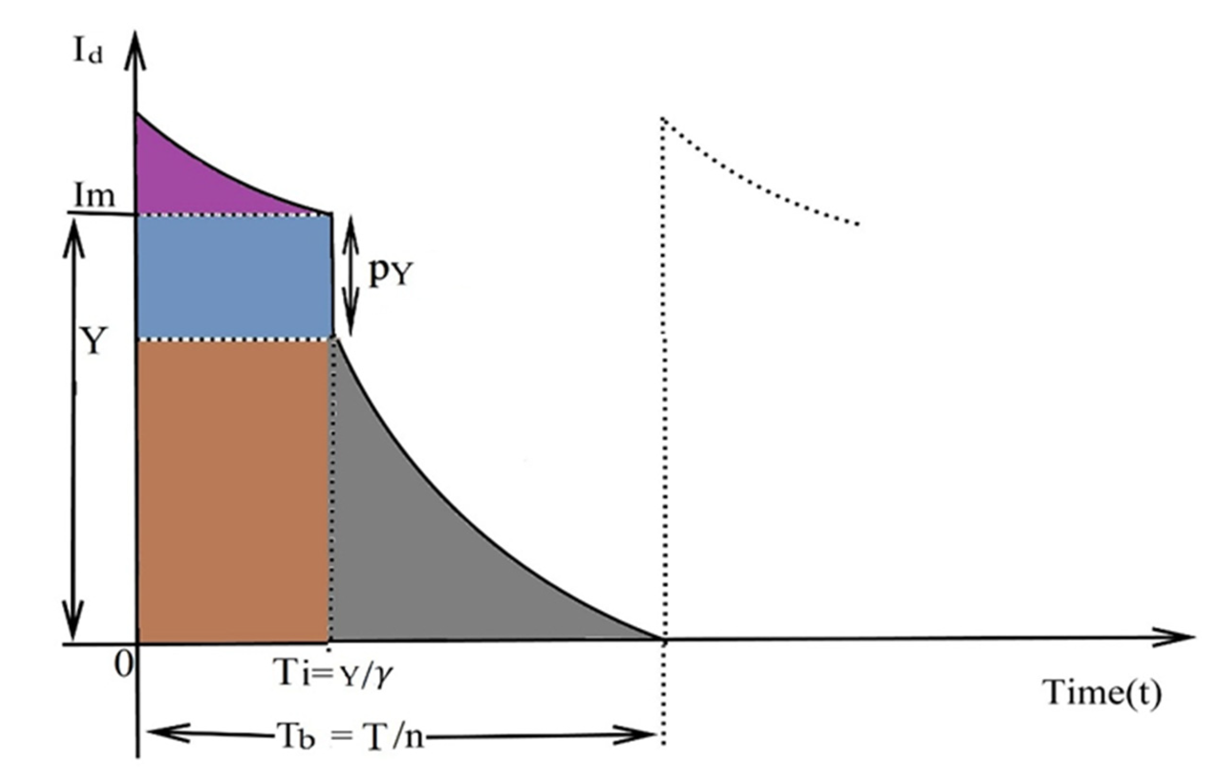
The manufacturer’s inventory level and retailer’s inventory level are presented in Figure 5 with suitable notations. It is supposed that the manufacturer produces units in one production cycle and also that the deliveries of these units to the retailer occur in shipment with a fixed lot Y. Then, the retailer inspects the whole received lot during the time period and obtains defective items.
The retailer removes all defective items from the level of inventory and also assumes that is the fixed screening cost per shipment. Let us consider that is the unit screening cost, as is suggested by Sarkar et al. [12]. The inventory level of the retailer reduces due the demand of the customer in the time period and the total screening cost per year.
From the literature review of Jaggi et al. [53], from the inventory level in the interval and , and from Figure 6,
and,
For solving from Equation (3), the value of if, then the value of (Jaggi et al. [53]),
The inventory level for the retailer from to ,
If the value of is replaced in Equation (5) from Equations (2) and (3), we obtain,
After simplifying Equation (6), we obtain,
As per consideration, the holding units require electrical energy with a fixed amount of carbon units or carbon footprint, so the value of from Equation (4) is replaced in Equation (7). Now, the holding cost per unit time is,
The carbon emission cost for the retailer is,
The deterioration cost per year for the retailer is,
The ordering cost for the retailer is,
The total inventory cost for the retailer, which is the sum of the total screening cost (), holding cost (), carbon emission cost (), deterioration cost and ordering cost is,
It is also considered that the expected probability value of the defective-quality products is . The retailer’s total cost is the sum of the ordering, inspection, deteriorating, inventory holding, and emission costs. Therefore, considering the probability of the defective products, the expected total cost per year is assessed from Equation (12).
3.2. Manufacturer Strategy under Cost and Carbon Emissions
When the retailer demands some products under some conditions from the manufacturer, then the manufacturer produces the demanded products with a production rate and the set up cost per production cycle is .
The manufacturer’s set up cost per year for the production is,
The first shipment lot goes ahead as soon as the demand is met and all deliveries arein the time interval .
The manufacturer includes the transportation cost, which is the sum of fixed and variable cost. The first part is the fixed transportation, the second part is the transportation cost when a vacant truck goes from the factory of the manufacturer to the retailer’s place and the truck returns to the factory of the manufacturer with the distance being twice the time (coming and going back with the same distance), and the third part depends on the loaded truck, additional fuels, and product weight. We were motivated by the literature reviews of some renowned authors who added the variable transportation cost in their research work, like Wangsaand Wee [65]., Rahman et al. [66], Nie et al. [67], and Swenseth and Godfrey [68],
If the value of from Equation (4) is replaced in Equation (15), we obtain,
During transportation, the delivery distance, actual shipment weight, fuel consumption per kilometer, and CO2 per liter of fuel are also responsible for the carbon emissions; we adopt the policies of Wahab et al. [10]. Considering the quantity of the carbon footprint for the manufacturer, we can calculate this.
Therefore, the amount of the manufacturer’s carbon emissions per year as a result of transportation activity can be derived as follows:
We studied many literature reviews concerning this study that worked on the theory of supply chain management, especially regarding the manufacturer’s strategy, like Lee and Kim [22], Yang and Wee’s [68], and Jayaswal et al. [59]. The retailer receives the demanded lot, which has some defective items, and for this reason, the retailer uses the policy of inspection. The demand rate of the manufacturer is . Therefore, the stock-level functions are obeyed and the work of this strategy is given in Figure 6.
By using the boundary condition = and adopting the strategy of Misra’s [59] approximation, we can write,
After solving the above equation, we obtain,
The holding inventory per cycle for the manufacturer is calculated by using the process of Yang and Wee [68],
We solve Equation (22), and after simplifying, then the holding cost per year for the manufacturer is,
The amount of carbon emissions for the manufacturer per year during warehousing activity is,
Considering the total carbon emissions cost per year for the manufacturer, from Equations (17) and (24), we obtain,
During the time period , there is a loss of inventory due to deterioration. The deterioration cost per year for the manufacturer is,
By using Equations (18), (23), (25), and (26) and also considering the probability of imperfect-quality items, the total expected cost per year for the manufacturer is,
The integrated total inventory cost for the supply chain from Equations (13) and (27) is,
4. Formulation of the Proposed Model under Fuzzy Environment
As per our assumptions, the demand rate is imprecise in nature and is also treated as a triangular fuzzy number. Equation (28) is converted from the crisp to fuzzy environment, then we obtain,
Now, we defuzzify Equation (29) with the help of the signed distance method, and the signed distance method between and is given by,
The signed distance from to can be defined (Patro et al. [54]) as,
As per consideration, the demand rate is considered as a triangular fuzzy number and we can write , where is a lower deviation and is an upper deviation of the demand rate. From Equation (31), we can write,
Equation (30) can be written by using Equation (32),
Now, we develop the present scenario under a learning environment and also consider the learning effect involved in the lower and upper deviation of the demand rate briefly discussed in the forthcoming section.
4.1. Formulation of the Proposed Model with Fuzzy Environment under Learning Effect
The learning effect is a cost reduction function and some authors have worked on this concept, like Wright [56], Patro et al. [54], and Jayaswal et al. [57]. The lower and upper deviation of the demand rate are related to learning and follow the formulation of Wright [56]. The mathematical shape of learning was presented by Wright [56] and is mathematically given below:
where is the time to prepare the -th units, is the time for opening , and is the learning slope. Now, we define the learning in the upper and lower deviation of the demand rate, which is given in Equations (35) and (36).
Now, the lower and upper deviation of the demand rate follow the effect of learning, then, Equation (33) can be written with the help of Equations (35) and (36), we obtain,
Note: we used Taylor’s series expansion in Equation (37) and neglected the higher term of the exponential series for the calculation of the cost function by using . The readers or researchers can consider a higher term like and this will be good for researchers, authors, and readers.
4.2. Methodology and Solution Method
We are following some steps for the calculation of decision variables, which are given below:
Step 1. Replace the values of and in Equations (20) and (21) in for the supply chain.
Step 2. Insert all values of the respective inventory parameters in cost Equation (37).
Step 3. Manage for the value of the shipment .
Step 4. The cost equation is partially differentiated with respect to and made equal to 0 for finding the value of Step 5. With the help of the value of we calculate the values of and by using the cost equation
Step 6. If then and go to Step 7, otherwise we manage and return to step 4.
Step 7. After using the optimal values of then we calculate .
5. Model Development with Manufacturer Inspection
The manufacturer delivers a product to the retailer after the inspection of the product and also improves the quality of the product by the using a screening process. The objective of the manufacturer is to stop the transportation of items of defective quality from the delivered lot to the retailer. The manufacturer inspects the whole lot after completing the production during the production time period and divides it into two categories, where one is defective-quality items and the other is non-defective items. The defective-quality items will be sold at a rebate price in another market and it is the policy for the manufacturer to improve the quality of the delivered lot. Supposing that is the inventory level for the manufecturer and is also the inventory level for the retailer, the level of defective product is for the manufacturer and the accumulated inventory level during time , and the level of decreases due to the demand for the product. The mathematical diagram of this is presented in Figure 7.
5.1. Retailer Cost and Emission
The cost function for the retailer is the sum of the holding cost for the inventory, ordering cost for the shipment, deterioration cost for the deterioration of the items, and emission cost to prevent the carbon units, and the working process of this model is same as the previous model. In this model, the ordering cost is considered as similar to model 1, and in the time period , the stock level decreases due to the demand and deterioration quality of the items (Figure 8). The value of the inventory level at time is considered with the help of Yang and Wee [69].
Now, the inventory level for this situation,
and,
The retailer’s holding cost per year is:
Further, the retailer’s deteriorating cost per year is:
The amount of carbon units from the holding units for the retailer is:
The carbon emission cost per year for the retailer due carbon units, from Equation (42) is:
The total expected cost for the retailer, , will be:
5.2. Manufacturer Cost and Emission
As per consideration, the manufacturer inspects the whole lot of produced items because produced lots have some defective items and the rate for the production of good-quality items is In Asper production cycle, the total number of items is . The set up cost per year for the manufacturer is and also includes some extra cost for the inspection process. Let us suppose that the fixed inspection cost per year is and unit inspection cost per year is .
Now, the total inspection cost per year for the manufacturer is:
The transportation cost is considered similar to the retailer as in model one.
The cost for the transportation and emissions of carbon units per year is:
With the boundary conditions of this equation, ,, and .
The inventory level for good-quality items for the manufacturer is:
For the calculation of , we use boundary condition , and from Equations (48) and (49), we obtain,
With the help of Taylor’s series expansion and considering in Equation (50), we follow the methodology of Misra’s [59] estimation,
Therefore, the inventory level for the good-quality items for the manufacturer is:
On the other hands, for the level of defective items, with the differential equation and from Figure 6, we can write the differential equation for defective-quality items:
With the boundary condition at ,
Now, the inventory function for the defective quality items for the manufacturer is:
The total amount of the defective products is:
Now, the holding cost per year for the manufacturer is:
And from Equations (47) and (55), the carbon emission cost and also the whole expected carbon emission cost for the manufacturer per year are:
Similarly, we calculated the deterioration cost per year for the manufacturer:
The total expected cost per year due to the probability of the defective-quality items for the manufacturer and similar methodology to the model one is:
5.3. Proposed Model under Fuzzy Environment
As per consideration, the demand rate is taken as a fuzzy demand rate and Equation (59) is converted into a fuzzy environment, then, we can write Equation (59):
Now, Equation (44) represents the retailer’s total cost in a crisp environment and we convert it into a fuzzy environment by taking the demand rate as a fuzzy demand rate, and we obtain,
The joint total fuzzy cost for the supply chain.
The joint total fuzzy cost is the sum of the total fuzzy cost of the retailer and manufacturer and by adding Equations (60) and (61), we obtain,
Now, the joint total fuzzy cost function from Equation (62), defuzzified with the help of the signed distance method (the signed distance from from can be defined (Patro et al. [54]):
We obtain
We replace the value of the in Equation (63), similar to model 1, and we obtain,
As per assumption, the lower and upper deviations of the demand rate follow the effect of the learning, which are defined in (32) and (33); now, we apply the concept of learning in Equation (64), and we obtain,
5.4. Methodology and Solution Method
For the calculation of decision variables, we follow some steps which are given below:
Step 1. Replace the values of and in Equations (51) and (52) in for the supply chain.
Step 2. Insert all values of the respective inventory parameters in the cost Equation (65).
Step 3. Manage for the value of the shipment .
Step 4. The cost equation is partially differentiated with respect to and made equal to 0 for the finding the value of .
Step 5. With the help of value of , we calculate the values of and by using the cost equation.
Step 6. If then and go to the Step 7, otherwise we manage and return to step 4.
Step 7. After using the optimal values of we calculate .
5.5. Numerical Example for Model 1 and 2
In this section, the input parameters are used in model 1 and model 2 from the literature reviews of Gautam and Khanna [14], Tiwari et al. [15], Salameh and Jaber [18], Goyal et al. [20], and Wee et al. [21]. The notation of the input parameters and the values are presented in Table 2.
As per consideration, the defective proportion in the delivered lot and the defective proportion obey the uniformly probability distribution (UPD) and we can define it as:
5.5.1. Numerical Example and Convexity of the Joint Total Fuzzy Cost for Model 1
With the help of the solution method under model 1, we calculate the minimum value of the joint fuzzy total cost for the supply chain under learning in fuzzy to be, at (Figure 9).
In model 1, if the learning and fuzzy environment are not included, it means that, the and the total cost for the supply chain is . Finally, model 1 is more effective with a learning and fuzzy environment. The combination of the learning and fuzzy environments is more beneficial for the proposed model.
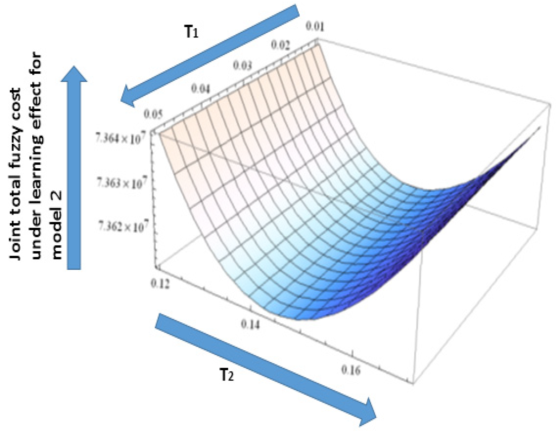
5.5.2. Numerical Example and Convexity of the Joint Total Fuzzy Cost for the Model 2
With the help of the solution method under model 2, we calculate the minimum value of the joint fuzzy total cost for the supply chain under learning in fuzzy to be, at (Figure 10).
In model 2, if the learning and fuzzy environment are not included, it means that, the and the total cost for the supply chain is . Finally, model 2 is more effective with a learning and fuzzy environment. The combination of the learning and fuzzy is more beneficial for the proposed model. Model 1 and model 2 are differentiated on the basis of the shipment, cycle time and total fuzzy cost, but in model 1, the total fuzzy cost is more than model 2 and this is presented in Table 3. This means that model 2 has more potential than model 1 on the basis of the cycle time and total fuzzy cost and this is the major difference between model 1 and 2.
From Table 3, we observe that the optimal number of shipments, cycle time, and integrated total fuzzy cost for model 1 are greater than model 2. In model 1, only the retailer inspects the whole received lot from the manufacturer under a fuzzy environment, whereas in model 2, the manufacturer inspects the whole lot before the delivery of the demanded items to the retailer under a fuzzy environment. Model 2 is more beneficial than model 1with respect to the shipments, cycle time, and integrated total fuzzy cost from the supply chain point of view when both players (retailer and manufacturer) inspect the whole lot, where the demand rate follows a triangular fuzzy number (Figure 11).
6. Sensitivity Analysis
In this section, we discuss and observe the effect of the inventory parameters of the proposed model on the supply chain’s total fuzzy cost under the decision variables. The sensitivity analysis needs to know about the sensitivity of the input parameters concerning the proposed model. The changeable effects of the inventory parameters on the supply chain’s total fuzzy cost under the decision variables are given inthe Table 4, Table 5, Table 6, Table 7, Table 8, Table 9, Table 10, Table 11, Table 12, Table 13, Table 14, Table 15 and Table 16.
6.1. Observation and Managerial Insights
- ➢
- By using Table 4, we concluded that from model1 and model 2, if the production rate of items increases then the number of shipments is fixed and the cycle time for the supply chain decreases, but the supply chain’s total fuzzy cost increases. This means that the production rate affects the cycle time and total fuzzy cost for the supply chain.
- ➢
- By using Table 5, we concluded that, from model 1 and model 2, if the fuzzy demand rate of items increases, then the number of shipments is fixed and the cycle time for the supply chain decreases, but the supply chain’s total fuzzy cost increases. This means that the fuzzy demand rate affects the cycle time and total fuzzy cost for the supply chain. It means that the fuzzy demand rate is a more sensitive parameter in the supply chain.
- ➢
- By using Table 6, we concluded that, from model 1 and model 2, if the values of learning rate increase, then the values of the shipments and cycle time increase, but the supply chain’s total fuzzy cost decreases up to when the learning rate moves from 0.150 to 0.154, but when the values of the learning rate increase after 0.154, then the shipments, cycle time, and supply chain’s total cost are fixed in position. This means that the learning rate affects the shipments, cycle time, and total fuzzy cost in the supply chain. Therefore, the learning effect is more effective for the decisions of the cycle time, number of shipments, and total fuzzy cost for model 1 and model 2, and also makes suggestions for the decision maker during the supply chain or ordering policies, etc. The learning fuzzy theory designs the numeric shape of the decision variables for the supply chain that we discuss in the model, like the cycle time, number of shipments, and lot size for model 1 and model 2.
- ➢
- By using Table 7 and Table 8, we concluded that, from model 1 and model 2, if the values of the unit screening cost and variable screening cost increase, then the values of the shipments and cycle time are fixed, but the supply chain’s total fuzzy cost increases. This means that the learning rate affects only the total fuzzy cost, but shipments, cycle time, and total fuzzy cost for the supply chain remain constant. This means that the shipment is independent from the inspection cost and the inspection process does not affect the shipment.
- ➢
- By using Table 9, we concluded that, from model 1 and model 2, if the deterioration rate increases, then the values of the shipment remain constant and the cycle time and supply chain’s total fuzzy cost increase.
- ➢
- By using Table 10, we concluded that, from model 1 and model 2, if the expected percentage defective increases, then the values of the shipment remain constant and the cycle time decreases, but the supply chain’s total fuzzy cost increases. It is also a sensitive parameter regarding cycle time and total fuzzy cost.
- ➢
- By using Table 11, we concluded that, from model 1 and model 2, if the carbon taxation increases, then the values of the shipment and cycle time remain constant, but the supply chain’s total fuzzy cost increases.
- ➢
- By using Table 12, we concluded that, from model 1 and model 2, if the manufacturer’s fixed transportation cost increases, then initially, the shipment and cycle time remain constant, but the supply chain’s total fuzzy cost increases. However, if the values of the manufacturer’s fixed transportation cost increase then the cycle time increases, but the shipments and total fuzzy cost decrease. Model 1 includes the transportation cost because the retailer pays the delivery charges when they receive the ordered lot and this cost saves the profit from the customer.
- ➢
- By using Table 13, we concluded that, from model 1 and model 2, if the manufacturer’s variable transportation cost increases, then initially, the shipments and cycle time remain constant, but the supply chain’s total fuzzy cost increases. However, if the values of the manufacturer’s variable transportation cost increase, then the cycle time increases but the shipments and total fuzzy cost decrease.
- ➢
- By using Table 14, we concluded from that, model 1 and model 2, if the product weight increases, then initially, the shipments and cycle time remain constant, but the supply chain’s total fuzzy cost increases.
- ➢
- By using Table 15, we concluded that, from model1 and model 2, if the average vehicle fuel consumption when there is no loading increases, then initially, the shipments and cycle time remain constant, but the supply chain’s total fuzzy cost increases.
- ➢
- By using Table 16, we concluded that, from model 1 and model 2, if the average additional fuel consumption with the loading of the items increases, then initially, the shipments and cycle time remain constant, but the supply chain’s total fuzzy cost increases.
6.2. Comparison of Proposed Model with Existing Model
In this section, we analyze our results against other contributions in this field. We provide in Table 17 selected author’s contributions who calculated the profit/cost for the ordering policies and the proposed model calculation of the total fuzzy cost with respect to the shipment and cycle time for model 1 and model 2. Our calculations for cycle time, shipment, lot size, and total fuzzy cost are presented at the bottom of Table 17.
7. Conclusions
The presented scenario assumes a two-level supply chain model with learning fuzzy theory for imperfect deteriorating items under carbon emissions, where both players (seller and buyer) inspect the whole lot with the help of an inspection process. The learning fuzzy theory is more beneficial for model 1 and model 2 during the two-level supply chain for the reduction in the carbon emissions, because it affects directly on the lot size of the integrated model. The deviation of fuzzy demand affects the total integrated fuzzy cost and it is the most effective inventory parameter. The impact of the carbon emissions, the rate of deterioration, two choices of inspection, rate of learning, shipments, and the deviation of the fuzzy demand are analyzed. We included different examples for each model and these are also reflected in the application of the proposed study. For managerial observations, we showed some results regarding inventory parameters, which are more important for the decision maker during the planning of a new type of business start. It is also observed that the number of shipments of delivered imperfect deteriorating items from the manufacturer is less when the vender inspects the whole lot under fuzzy learning and carbon emissions. Finally, the whole fuzzy cost of the supply chain is less due to the decrease in the whole holding cost and whole deterioration cost. However, the vender’s whole cost will be higher when the vender uses the policy of inspection. Therefore, both players receive profit during supply chain management under fuzzy learning theory. The novelty of this proposed model is that the total fuzzy cost for the supply chain system is less when the vendor uses the screening process. The proposed study finding also explained that, though the total fuzzy cost is minimum when the screening (double screening process) is performed by both players, it does not ensure a minimization of carbon emissions. However, for both members, the cost-saving and emission reduction aims can be obtained simultaneously by minimizing the level of the fuzzy cost saving. In this case, there is a tradeoff between fuzzy cost saving and minimizations in carbon emissions. The vendor’s total fuzzy cost becomes higher when they perform screening. Therefore, the retailer is required to compensate for a definite amount of cost saving for the manufacturer so that both players make profit. By using Table 11, we concluded from model1 and model 2 that the fuzzy total cost was affected by the carbon emissions, because the government includes higher carbon taxation for more carbon emissions. If carbon taxation increases, then the values of the shipment and cycle time remain constant, but the supply chain’s total fuzzy cost increases. The carbon emissions can be controlled by using less transportation, because transportation produces more and more carbon emissions during the supply of the product via vehicles from one place to another place. The presented proposed model calculated the minimum shipment for the supply chain under such assumptions and also saved transportation costs, as well as produced less carbon emissions.
7.1. Application and Future Scope of Proposed Model
The application of the proposed model is more applicable in the online market (like Amazone and Flipkart), food factories, big bazars, or supermarkets, as well as the storage of perishable items or those items which have a greater deteriorating rate. In such sectors, retailers or buyer inspect the whole lot of items and classify the whole lot into defective or non-defective items. Defective quality items are sold at a low price because they are damaged in a very short time. Finally, this model is more beneficial for online-based markets who sell eco-friendly food items like burgers, pizza, and other delivery-based items. The application of fuzzy learning theory had a positive effect on the ordering policies of the lot size for the supply of imperfect deteriorating items during the two-level supply chain with the effect of the supply chain. The proposed model covers a great scope of supply chain management and also deals with carbon emissions. The scope of this model has a wide opportunity to be improved by using this approach for three-level supply chain management. Future scopes can assume a rework system under an inspection environment and this will also be useful considering the nice contributions of Ji et al. [69] and Ji and Ma [70].
7.2. Limitation of Proposed Model
The proposed models, namely model1 and model 3, will be more and more applicable in the business sector or industrial firms, as well as in online markets, if the decision maker follows the model’s assumptions and also takes the numerical values of the input parameters. The proposed model has some limitations: (i) the double screening process should be executed during the supply chain, (ii) the range of the fuzzy demand rate should be according to numerical examples also discussed in the sensitivity analysis, (iii) the value of the learning should be according to the numerical example, and (iv) the item should be a deteriorating/perishable item, and also, the rate of the deterioration of the item should be according to the proposed model.
Author Contributions
Conceptualization, B.S.O.A. and M.H.A.; methodology, B.S.O.A. and M.H.A.; investigation, B.S.O.A.; writing—original draft, B.S.O.A. and M.H.A.; writing—review & editing, B.S.O.A. All authors have read and agreed to the published version of the manuscript.
Funding
This research received no external funding.
Data Availability Statement
The data presented in this study are available on request from the corresponding author.
Acknowledgments
The authors express sincere thanks to the editor and the anonymous reviewers for their valuable and constructive fruitful comments and suggestions, which led to a significant improvement of an earlier version of the manuscript.
Conflicts of Interest
The authors declare no conflict of interest.
Notations
| The rate of the demand (unit per year); | |
| The rate of the fuzzy demand (unit per year); | |
| Lower deviation of the fuzzy demand (unit per year); | |
| Upper deviation of the fuzzy demand (unit per year) | |
| The rate of the production of the deteriorating items (unit per year); | |
| Manufacturer’s production period of the product in each cycle (year); | |
| The quantity for the production (units); | |
| Defective percentage items in each delivered lot; | |
| The rate of the deterioration of the product ; | |
| Screening rate of quality (unit per year); | |
| Fixed inspection rate for the quality (USD per year); | |
| The cost for unit screening items (USD per year); | |
| Ordering cost for the retailer (USD per shipment); | |
| Holding cost for the retailer (USD per unit per year); | |
| Deterioration cost for the retailer (unit per year); | |
| Set up cost for the manufacturer (USD per shipment); | |
| Holding cost for the manufacturer (USD per unit per year); | |
| Deterioration cost for the manufacturer (unit per year); | |
| Fixed transportation cost for the manufacturer (unit per delivery); | |
| Fuel cost for manufacturer’s change able transportation cost (USD per liter); | |
| Distance covered from the seller to buyer (Km); | |
| The weight of the product; | |
| The average vehicle fuel consumption when does not use any fuel (liter per Km); | |
| Extra or average additional fuel consumption per ton of load (liter per kilometer per ton); | |
| The tax for the carbon emissions (USD per ton CO2); | |
| Average carbon emissions due to burning of fuel (ton CO2 per liter); | |
| Average carbon emissions due to electricity generation (ton CO2 per kWh); | |
| Carbon emission cost due to transportation (USD per kilometer); | |
| Carbon emission cost per unit item due to average additional transportation (USD per unit per Km; | |
| Average carbon emissions from the warehouses of per unit item (kWh per unit per year); | |
| Carbon emission cost due to warehouse of unit per item (USD per unit per year); | |
| Cycle time (year); | |
| No production period for manufacturer; | |
| Inspection time period for each delivery for retailer; | |
| Cycle time per delivery for the retailer (year); | |
| Inventory level for the manufacturer at time ; | |
| Inventory level for the manufacturer due to defective items at time ; | |
| Inventory level for the retailer at time | |
| Retailer’s total expected cost; | |
| Manufacturer’s total expected cost; | |
| Integrated total inventory cost; | |
| Integrated total fuzzy cost; | |
| Integrated total fuzzy cost under learning effect; | |
| Retailer’s total expected cost under carbon emissions; | |
| Manufacturer’s total expected cost under carbon emissions; | |
| Integrated total expected cost under carbon emissions; | |
| Integrated total expected fuzzy cost under carbon emissions; | |
| Integrated total expected cost under carbon emissions and learning in fuzzy; | |
| Lot size for the supply chain (variable decision); | |
| Number of shipment (variable decision); |
References
- Glock, C.H. The joint economic lot size problem: A review. Int. J. Prod. Econ. 2012, 135, 671–686. [Google Scholar] [CrossRef]
- Luo, Z.; Gunasekaran, A.; Dubey, R.; Childe, S.J.; Papadopoulos, T. Antecedents of low carbon emissions supply chains. Int. J. Clim. Chang. Strateg. Manag. 2017, 9, 707–727. [Google Scholar] [CrossRef]
- Das, C.; Jharkharia, S. Low carbon supply chain: A state-of-the-art literature review. J. Manuf. Technol. Manag. 2018, 29, 398–428. [Google Scholar] [CrossRef]
- Kazemi, N.; Abdul-Rashid, S.H.; Ghazilla, R.A.R.; Shekarian, E.; Zanoni, S. Economic order quantity models for items with imperfect quality and emission considerations. Int. J. Syst. Sci. Oper. Logist. 2018, 5, 99–115. [Google Scholar] [CrossRef]
- Sarkar, B.; Ahmed, W.; Choi, S.B.; Tayyab, M. Sustainable inventory management for environmental impact through partial backordering and multi-trade-credit period. Sustainability 2018, 10, 4761. [Google Scholar] [CrossRef]
- Taleizadeh, A.A.; Soleymanfar, V.R.; Govindan, K. Sustainable economic production quantity models for inventory system with shortage. J. Clean. Prod. 2018, 174, 1011–1020. [Google Scholar] [CrossRef]
- Sarkar, B.; Ganguly, B.; Sarkar, M.; Pareek, S. Effect of variable transportation and carbon emission in a three-echelon supply chain model. Transp. Res. Part E Logist. Transp. Rev. 2016, 91, 112–128. [Google Scholar] [CrossRef]
- Sarkar, B.; Ahmed, W.; Kim, N. Joint effects of variable carbon emission cost and multi-delay-in-payments under single-setup-multiple-delivery policy in a global sustainable supply chain. J. Clean. Prod. 2018, 185, 421–445. [Google Scholar] [CrossRef]
- Daryanto, Y.; Wee, H.M. Single vendor-buyer integrated inventory model for deteriorating items considering carbon emission. In Proceedings of the 8th International Conference on Industrial Engineering and Operations Management (IEOM), Bandung, Indonesia, 6–8 March 2018; pp. 544–555. [Google Scholar]
- Wahab, M.I.M.; Mamun, S.M.H.; Ongkunarak, P. EOQ models for a coordinated two-level international supply chain considering imperfect items and environmental impact. Int. J. Prod. Econ. 2011, 134, 151–158. [Google Scholar] [CrossRef]
- Jauhari, W.A.; Pamuji, A.S.; Rosyidi, C.N. Cooperative inventory model for vendor-buyer system with unequal-sized shipment, defective items and carbon emission cost. Int. J. Logist. Syst. Manag. 2014, 19, 163–186. [Google Scholar] [CrossRef]
- Sarkar, B.; Saren, S.; Sarkar, M.; Seo, Y.W. A Stackelberg game approach in an integrated inventory model with carbon-emission and setup cost reduction. Sustainability 2016, 8, 1244. [Google Scholar] [CrossRef]
- Jauhari, W.A. A collaborative inventory model for vendor-buyer system with stochastic demand, defective items and carbon emission cost. Int. J. Logist. Syst. Manag. 2018, 29, 241–269. [Google Scholar]
- Gautam, P.; Khanna, A. An imperfect production inventory model with setup cost reduction and carbon emission for an integrated supply chain. Uncertain Supply Chain Manag. 2018, 6, 271–286. [Google Scholar] [CrossRef]
- Tiwari, S.; Daryanto, Y.; Wee, H.M. Sustainable inventory management with deteriorating and imperfect quality items considering carbon emissions. J. Clean. Prod. 2018, 192, 281–292. [Google Scholar] [CrossRef]
- Rosenblatt, M.J.; Lee, H.L. Economic production cycles with imperfect production processes. IIE Trans. 1986, 18, 48–55. [Google Scholar] [CrossRef]
- Porteus, E.L. Optimal lot sizing, process quality improvement and setup cost reduction. Oper. Res. 1986, 34, 137–144. [Google Scholar] [CrossRef]
- Salameh, M.K.; Jaber, M.Y. Economic production quantity model for items with imperfect quality. Int. J. Prod. Econ. 2000, 64, 59–64. [Google Scholar] [CrossRef]
- Huang, C.K. An integrated vendor-buyer cooperative inventory model for items with imperfect quality. Prod. Plan. Control 2002, 13, 355–361. [Google Scholar] [CrossRef]
- Goyal, S.K.; Huang, C.K.; Chen, K.C. A simple integrated production policy of an imperfect item for vendor and buyer. Prod. Plan. Control 2003, 14, 596–602. [Google Scholar] [CrossRef]
- Wee, H.M.; Yu, J.C.P.; Wang, K.J. An integrated production-inventory model for deteriorating items with imperfect quality and shortage backordering considerations. In Proceedings of the International Conference on Computational Science and Its Applications (ICCSA), Glasgow, UK, 8–11 May 2006; Springer: Berlin/Heidelberg, Germany, 2006; pp. 885–897. [Google Scholar]
- Lee, S.; Kim, D. An optimal policy for a single vendor single-buyer integrated production-distribution model with both deteriorating and defective items. Int. J. Prod. Econ. 2014, 147, 161–170. [Google Scholar] [CrossRef]
- Bazan, E.; Jaber, M.Y.; Zanoni, S.; Zavanella, L.E. Vendor managed inventory (VMI) with consignment stock (CS) agreement for a two-level supply chain with an imperfect production process with/without restoration interruptions. Int. J. Prod. Econ. 2014, 157, 289–301. [Google Scholar] [CrossRef]
- Sarkar, B.; Shaw, B.K.; Kim, T.; Sarkar, M.; Shin, D. An integrated inventory model with variable transportation cost, two-stage inspection, and defective items. J. Ind. Manag. Optim. 2017, 13, 1975–1990. [Google Scholar] [CrossRef]
- Yu, H.F.; Hsu, W.K. An integrated inventory model with immediate return for defective items under unequal-sized shipments. J. Ind. Prod. Eng. 2017, 34, 70–77. [Google Scholar] [CrossRef]
- Benjaafar, S.; Li, Y.; Daskin, M. Carbon footprint and the management of supply chains: Insights from simple models. IEEE Trans. Autom. Sci. Eng. 2013, 10, 99–116. [Google Scholar] [CrossRef]
- Fahimnia, B.; Sarkis, J.; Dehghanian, F.; Banihashemi, N.; Rahman, S. The impact of carbon pricing on a closed-loop supply chain: An Australian case study. J. Clean. Prod. 2013, 59, 210–225. [Google Scholar] [CrossRef]
- Bozorgi, A.; Pazour, J.; Nazzal, D. A new inventory model for cold items that considers costs and emissions. Int. J. Prod. Econ. 2014, 155, 114–125. [Google Scholar] [CrossRef]
- Bozorgi, A. Multi-product inventory model for cold items with cost and emission consideration. Int. J. Prod. Econ. 2016, 176, 123–142. [Google Scholar] [CrossRef]
- Ruidas, S.; Seikh, M.R.; Nayak, P.K. A production inventory model with interval-valued carbon emission parameters under price-sensitive demand. Compu. Ind. Eng. 2021, 154, 107154. [Google Scholar] [CrossRef]
- Ghosh, A.; Jha, J.K.; Sarmah, S.P. Optimizing a two-echelon serial supply chain with different carbon policies. Int. J. Sustain. Eng. 2016, 9, 363–377. [Google Scholar] [CrossRef]
- Toptal, A.; Çetinkaya, B. How supply chain coordination affects the environment: A carbon footprint perspective. Ann. Oper. Res. 2017, 250, 487–519. [Google Scholar] [CrossRef]
- Bouchery, Y.; Ghaffari, A.; Jemai, Z.; Tan, T. Impact of coordination on cost and carbon emissions for a two-echelon serial economic order quantity problem. Eur. J. Oper. Res. 2017, 260, 520–533. [Google Scholar] [CrossRef]
- Dwicahyani, A.R.; Jauhari, W.A.; Rosyidi, C.N.; Laksono, P.W. Inventory decisions in a two-echelon system with remanufacturing, carbon emission, and energy effects. Cogent Eng. 2017, 4, 1379628. [Google Scholar] [CrossRef]
- Li, J.; Su, Q.; Ma, L. Production and transportation outsourcing decisions in the supply chain under single and multiple carbon policies. J. Clean. Prod. 2017, 141, 1109–1122. [Google Scholar] [CrossRef]
- Wangsa, I.D. Greenhouse gas penalty and incentive policies for a joint economic lot size model with industrial and transport emissions. Int. J. Ind. Eng. Comput. 2017, 8, 453–480. [Google Scholar]
- Anvar, S.H.; Sadegheih, A.; Zad, M.A.V. Carbon emission management for greening supply chains at the operational level. Environ. Eng. Manag. J. 2018, 17, 1337–1347. [Google Scholar] [CrossRef]
- Hariga, M.; Babekian, S.; Bahroun, Z. Operational and environmental decisions for a two-stage supply chain under vendor managed consignment inventory partnership. Int. J. Prod. Res. 2018, 57, 3642–3662. [Google Scholar] [CrossRef]
- Ji, S.; Zhao, D.; Peng, X. Joint decisions on emission reduction and inventory replenishment with overconfidence and low-carbon preference. Sustainability 2018, 10, 1119. [Google Scholar] [CrossRef]
- Wang, S.; Ye, B. A comparison between just-in-time and economic order quantity models with carbon emissions. J. Clean. Prod. 2018, 187, 662–671. [Google Scholar] [CrossRef]
- Ghosh, A.; Sarmah, S.P.; Jha, J.K. Collaborative model for a two-echelon supply chain with uncertain demand under carbon tax policy. Sadhana 2018, 43, 144. [Google Scholar] [CrossRef]
- Ma, X.; Ho, W.; Ji, P.; Talluri, S. Coordinated pricing analysis with the carbon tax scheme in a supply chain. Decis. Sci. 2018, 49, 863–900. [Google Scholar] [CrossRef]
- Darom, N.A.; Hishamuddin, H.; Ramli, R.; Nopiah, Z.M. An inventory model of supply chain disruption recovery with safety stock and carbon emission consideration. J. Clean. Prod. 2018, 197, 1011–1021. [Google Scholar] [CrossRef]
- Huang, H.; He, Y.; Li, D. Pricing and inventory decisions in the food supply chain with production disruption and controllable deterioration. J. Clean. Prod. 2018, 180, 280–296. [Google Scholar] [CrossRef]
- Daryanto, Y.; Wee, H.M.; Astanti, R.D. Three-echelon supply chain model considering carbon emission and item deterioration. Transp. Res. Part E Logist. Transp. Rev. 2019, 122, 368–383. [Google Scholar] [CrossRef]
- Kundu, S.; Chakrabarti, T. A fuzzy rough integrated multi-stage supply chain inventory model with carbon emissions under inflation and time-value of money. Int. J. Math. Oper. Res. 2019, 14, 123–145. [Google Scholar] [CrossRef]
- Shalke, P.N.; Paydar, M.M.; Hajiaghaei-Keshteli, M. Sustainable supplier selection and order allocation through quantity discounts. Int. J. Manag. Sci. Eng. Manag. 2018, 13, 20–32. [Google Scholar]
- Moheb-Alizadeh, H.; Handfield, R. An integrated chance-constrained stochastic model for efficient and sustainable supplier selection and order allocation. Int. J. Prod. Res. 2018, 56, 6890–6916. [Google Scholar] [CrossRef]
- Moheb-Alizadeh, H.; Handfield, R. Sustainable supplier selection and order allocation: A novel multi-objective programming model with a hybrid solution approach. Comput. Ind. Eng. 2019, 129, 192–209. [Google Scholar] [CrossRef]
- Jaggi, C.K.; Sharma, A.; Mittal, M. A fuzzy inventory model for deteriorating items with initial inspection and allowable shortage under the condition of permissible delay in payment. Int. J. Invent. Control Manag. 2012, 2, 167–200. [Google Scholar] [CrossRef]
- Jaggi, C.K.; Pareek, S.; Sharma, A. A Fuzzy Inventory Model for Weibull Deteriorating Items with Price-Dependent Demand and Shortages under Permissible Delay in Payment. Inter. J. Appl. Indus. Eng. 2012, 1, 53–79. [Google Scholar] [CrossRef]
- Jaggi, C.K.; Sharma, A.; Jain, R. EOQ model with permissible delay in payments under fuzzy environment. In Analytical Approaches to Strategic Decision-Making: Interdisciplinary Considerations; IGI Global: Hershey, PA, USA, 2014; pp. 281–296. [Google Scholar]
- Rout, C.; Kumar, R.S.; Paul, A.; Chakraborty, D.; Goswami, A. Designing a single-vendor and multiple-buyers’ integrated production inventory model for interval type-2 fuzzy demand and fuzzy rule based deterioration. RAIRO-Oper. Res. 2021, 55, 3715–3742. [Google Scholar] [CrossRef]
- Patro, R.; Acharya, M.; Nayak, M.M.; Patnaik, S. A fuzzy EOQ model for deteriorating items with imperfect quality using proportionate discount under learning effects. Int. J. Manag. Decis. Mak. 2018, 17, 171–198. [Google Scholar] [CrossRef]
- Bhavani, G.D.; Meidute-Kavaliauskiene, I.; Mahapatra, G.S.; Činčikaitė, R.A. Sustainable Green Inventory System with Novel Eco-Friendly Demand Incorporating Partial Backlogging under Fuzziness. Sustainability 2022, 14, 9155. [Google Scholar] [CrossRef]
- Wright, T.P. Factors affecting the cost of airplanes. J. Aeronaut. Sci. 1936, 3, 122–128. [Google Scholar] [CrossRef]
- Jayaswal, M.K.; Mittal, M.; Alamri, O.A.; Khan, F.A. Learning EOQ Model with Trade-Credit Financing Policy for Imperfect Quality Items under Cloudy Fuzzy Environment. Mathematics 2022, 10, 246. [Google Scholar] [CrossRef]
- Jayaswal, M.K.; Mittal, M.; Sangal, I.; Tripathi, J. Fuzzy-Based EOQ Model with Credit Financing and Backorders Under Human Learning. Int. J. Fuzzy Syst. Appl. 2021, 10, 14–36. [Google Scholar] [CrossRef]
- Jayaswal, M.K.; Mittal, M. Impact of Learning on the Inventory Model of Deteriorating Imperfect Quality Items with Inflation and Credit Financing under Fuzzy Environment. Int. J. Fuzzy Syst. Appl. 2022, 11, 1–36. [Google Scholar] [CrossRef]
- Alamri, O.A.; Jayaswal, M.K.; Mittal, M. A Supply Chain Model with Learning Effect and Credit Financing Policy for Imperfect Quality Items under Fuzzy Environment. Axioms 2023, 12, 260. [Google Scholar] [CrossRef]
- Alamri, O.A. Sustainable Supply Chain Model for Defective Growing Items (Fishery) with Trade Credit Policy and Fuzzy Learning Effect. Axioms 2023, 12, 436. [Google Scholar] [CrossRef]
- Alsaedi, B.S.; Alamri, O.A.; Jayaswal, M.K.; Mittal, M. A sustainable green supply chain model with carbon emissions for defective items under learning in a fuzzy environment. Mathematics 2023, 11, 301. [Google Scholar] [CrossRef]
- Giri, B.K.; Roy, S.K. Fuzzy-random robust flexible programming on sustainable closed-loop renewable energy supply chain. Appl. Energy 2024, 363, 123044. [Google Scholar] [CrossRef]
- Hariga, M.; As’ad, R.; Shamayleh, A. Integrated economic and environmental models for a multi stage cold supply chain under carbon tax regulation. J. Clean. Prod. 2017, 166, 1357–1371. [Google Scholar] [CrossRef]
- Wangsa, I.D.; Wee, H.M. An integrated vendor-buyer inventory model with transportation cost and stochastic demand. Int. J. Syst. Sci. Oper. Logist. 2018, 5, 295–309. [Google Scholar]
- Rahman, M.N.A.; Leuveano, R.A.C.; bin Jafar, F.A.; Saleh, C.; Deros, B.M.; Mahmood, W.M.F.W.; Mahmood, W.H.W. Incorporating logistic costs into a single vendor-buyer JELS model. Appl. Math. Model. 2016, 40, 10809–10819. [Google Scholar] [CrossRef]
- Nie, L.; Xu, X.; Zhan, D. Incorporating transportation costs into JIT lot splitting decisions for coordinated supply chains. J. Adv. Manuf. Syst. 2006, 5, 111–121. [Google Scholar] [CrossRef]
- Yang, P.C.; Wee, H.M. Economic ordering policy of deteriorated item for vendor and buyer: An integrated approach. Prod. Plan. Control 2000, 11, 474–480. [Google Scholar] [CrossRef]
- Ji, Y.; Li, Y.; Wijekoon, C. Robust two-stage minimum asymmetric cost consensus models under uncertainty circumstances. Inf. Sci. 2024, 120279. [Google Scholar] [CrossRef]
- Ji, Y.; Ma, Y. The robust maximum expert consensus model with risk aversion. Inf. Fusion 2023, 99, 101866. [Google Scholar] [CrossRef]
Figure 1.
Inspection system under vendor production.

Figure 2.
Inspection system under retailer system.

Figure 3.
Presentation of methodology of the proposed model through flowchart.

Figure 4.
Representation of the average fuel consumption.

Figure 5.
Manufacturer’s and retailer’s model for deteriorating items.

Figure 6.
Retailer’s model for deteriorating items under inspection process.

Figure 7.
Representation of production and non-production process for the manufacturer.

Figure 8.
Manufacturer’s and retailer’s model for constant deteriorating items under inspection process.
Figure 8.
Manufacturer’s and retailer’s model for constant deteriorating items under inspection process.

Figure 9.
The convexity of the joint total fuzzy cost under learning effect for model 1.

Figure 10.
The convexity of the joint total fuzzy cost under learning effect for model 2.

Figure 11.
Comparison of model 1 and model 2 with respect to the joint total fuzzy cost under learning effect.
Figure 11.
Comparison of model 1 and model 2 with respect to the joint total fuzzy cost under learning effect.


Table 1.
Contribution of the authors and proposed work.
| Author | Supply Chain | Vender’s Inspection | Buyer’s Inspection | Carbon Emissions | Deteriorating Items | Imperfect Items and Inspection | Learning in Inspection | Learning in Fuzzy Environment |
|---|---|---|---|---|---|---|---|---|
| Wright [56] | ✔ | |||||||
| Salameh and Jaber [18] | ✔ | |||||||
| Tiwari et al. [15] | ✔ | ✔ | ✔ | ✔ | ||||
| Bazan et al. [23] | ✔ | ✔ | ||||||
| Wangsa [36] | ✔ | ✔ | ||||||
| Daryantoet al. [45] | ✔ | ✔ | ✔ | ✔ | ||||
| Jaggi et al. [50] | ✔ | |||||||
| Patro et al. [54] | ✔ | ✔ | ✔ | |||||
| Jayaswal et al. [59] | ✔ | ✔ | ✔ | |||||
| Almari [61] | ✔ | ✔ | ||||||
| Alsaedi et al. [62] | ✔ | ✔ | ✔ | ✔ | ||||
| Giri and Roy [63] | ✔ | Nice contribution in fuzzy environment and did not work with learning | ||||||
| Proposed model | ✔ | ✔ | ✔ | ✔ | ✔ | ✔ | ✔ | ✔ |
Table 2.
Model’s input parameters.
| Inventory Parameters | Values with Unit | Inventory Parameters | Values with Unit |
|---|---|---|---|
| 2,000,000 units per year | USD 2000 per order | ||
| 50,000 units per year | USD 100,000 per setup | ||
| 1,725,000 unit per year | USD 60 per unit per year | ||
| USD 500 per delivery | USD 40 per unit per year | ||
| USD 0.5 per unit | USD 600 per unit | ||
| 0.10 | USD 400 per unit | ||
| USD 1000 per delivery | 100 km | ||
| USD 0.75 per liter | 0.01 ton per unit | ||
| 1.44 kwh per hour unit per year | 27 L per 100 km | ||
| USD 75 per ton | 0.57 L per 100 km per ton truck load | ||
| ton C per liter | 0 | ||
| ton C per kwh | 0.04 with | ||
| 4 |
Table 3.
Comparison of model1 and model 2.
| Model 1 | Model 2 | ||||||||
|---|---|---|---|---|---|---|---|---|---|
| 3 | USD | 5 | USD | ||||||
Table 4.
Impact of production rate on the supply chain’s total cost under decision variables.
| Input Parameter | Model I | Model II | ||||||||
|---|---|---|---|---|---|---|---|---|---|---|
| 2,000,000 | 3 | 5 | USD | |||||||
| 2,100,000 | 3 | 0.11006 | 5 | 0.17385 | USD | |||||
| 2,200,000 | 3 | 0.10774 | 5 | 0.1721 | USD | |||||
Table 5.
Impact of fuzzy demand rate on the supply chain’s total cost under decision variables.
| Input Parameter | Model I | Model II | ||||||||
|---|---|---|---|---|---|---|---|---|---|---|
| 3 | 5 | USD | ||||||||
| 5 | 0.11023 | 7 | 0.17305 | USD | ||||||
| 5 | 0.10674 | 7 | 0.1715 | USD | ||||||
Table 6.
Impact of learning rate on the supply chain’s total cost under decision variables.
| Input Parameter | Model I | Model II | ||||||||
|---|---|---|---|---|---|---|---|---|---|---|
| 1 | 0.10189 | 2 | 0.17206 | USD | ||||||
| 2 | 0.10619 | 3 | 0.17407 | USD | ||||||
| 3 | 5 | USD | ||||||||
| 0.153 | 3 | 5 | USD | |||||||
| 0.154 | 3 | 5 | USD | |||||||
Table 7.
Impact of unit screening cost on the supply chain’s total cost under decision variable.
| Input Parameter | Model I | Model II | ||||||||
|---|---|---|---|---|---|---|---|---|---|---|
| 3 | 0.10374 | 5 | 0.17077 | USD | ||||||
| 3 | 0.10671 | 5 | 0.17465 | USD | ||||||
| 3 | 5 | USD | ||||||||
Table 8.
Impact of unit variable screening cost on the supply chain’s total cost under decision variable.
Table 8.
Impact of unit variable screening cost on the supply chain’s total cost under decision variable.
| Input Parameter | Model I | Model II | ||||||||
|---|---|---|---|---|---|---|---|---|---|---|
| 3 | 5 | USD | ||||||||
| 3 | 5 | USD | ||||||||
| 3 | 5 | USD | ||||||||
Table 9.
Impact of deteriorating rate on the supply chain’s total cost under decision variable.
| Input Parameter | Model I | Model II | ||||||||
|---|---|---|---|---|---|---|---|---|---|---|
| 3 | 0.11295 | 5 | 0.18206 | USD | ||||||
| 3 | 0.11270 | 5 | 0.18075 | USD | ||||||
| 3 | 5 | USD | ||||||||
Table 10.
Impact of expected percentage defective on the supply chain’s total cost under decision variable.
Table 10.
Impact of expected percentage defective on the supply chain’s total cost under decision variable.
| Input Parameter | Model I | Model II | ||||||||
|---|---|---|---|---|---|---|---|---|---|---|
| 3 | 5 | USD | ||||||||
| 3 | 0.11200 | 5 | 0.17435 | USD | ||||||
| 3 | 0.11118 | 5 | 0.17257 | USD | ||||||
Table 11.
Impact of carbon taxation on the supply chain’s total cost under decision variable.
| Input Parameter | Model I | Model II | ||||||||
|---|---|---|---|---|---|---|---|---|---|---|
| 3 | 5 | USD | ||||||||
| 3 | 5 | USD | ||||||||
| 3 | 5 | USD | ||||||||
Table 12.
Impact of carbon average warehouse energy consumption on the supply chain’s total cost under decision variables.
Table 12.
Impact of carbon average warehouse energy consumption on the supply chain’s total cost under decision variables.
| Input Parameter | Model I | Model II | ||||||||
|---|---|---|---|---|---|---|---|---|---|---|
| 3 | 5 | USD | ||||||||
| 3 | 5 | USD | ||||||||
| 3 | 5 | USD | ||||||||
Table 13.
Impact of manufacturer’s fixed transportation cost on the supply chain’s total cost under decision variables.
Table 13.
Impact of manufacturer’s fixed transportation cost on the supply chain’s total cost under decision variables.
| Input Parameter | Model I | Model II | ||||||||
|---|---|---|---|---|---|---|---|---|---|---|
| 3 | 5 | USD | ||||||||
| 3 | 4 | USD | ||||||||
| 2 | 3 | USD | ||||||||
Table 14.
Impact of manufacturer’s variable transportation cost on the supply chain’s total cost under decision variables.
Table 14.
Impact of manufacturer’s variable transportation cost on the supply chain’s total cost under decision variables.
| Input Parameter | Model I | Model II | ||||||||
|---|---|---|---|---|---|---|---|---|---|---|
| 3 | 5 | USD | ||||||||
| 3 | 4 | USD | ||||||||
| 2 | 3 | USD | ||||||||
Table 15.
Impact of product weight on the supply chain’s total cost under decision variables.
| Input Parameter | Model I | Model II | ||||||||
|---|---|---|---|---|---|---|---|---|---|---|
| 3 | 5 | USD | ||||||||
| 3 | 5 | USD | ||||||||
| 3 | 5 | USD | ||||||||
Table 16.
Impact of average additional fuel consumption on the supply chain’s total cost under decision variables.
Table 16.
Impact of average additional fuel consumption on the supply chain’s total cost under decision variables.
| Input Parameter | Model I | Model II | |||||||||
|---|---|---|---|---|---|---|---|---|---|---|---|
| 0.0057 | 3 | 5 | USD | ||||||||
| 0.0058 | 3 | 5 | USD | ||||||||
| 0.0059 | 3 | 5 | USD | ||||||||
Table 17.
Comparison of results (existing model) with our proposed model.
| Author’s Name | Double Screening Process | Learning Fuzzy Thery | Lot Size | Cycle Time as a Decision Variable | Shipment as a Decision Variable | Total Profit/Total Cost under EOQ/EPQ/Supply Chain |
|---|---|---|---|---|---|---|
| Salsmeh and Jaber [18] | Not calculated | Not calculated | 1439 units | Not calculated | Not calculated | USD 1,212,235 |
| Yu et al. [25] | Not calculated | Not calculated | 1288 units | Not calculated | Not calculated | USD 1,212,148 |
| Jaggi et al. [52] | Not calculated | Not calculated | 1642 units | Not calculated | Not calculated | USD 347,086 |
| Patro et al. [54] | Not calculated | Not calculated | 1117 units | Not calculated | Not calculated | USD 1,273,420 |
| Alamri et al. [60] | Not calculated | Not calculated | 48225 units | Not calculated | Not calculated | USD 1,662,440 |
| Our paper under supply chain for model 1 | Yes | Yes | 6198 units | 0.11248 Year | Calculated, 3 | Total inventory fuzzy cost for the supply chain USD 8,220,400 |
| Our paper under supply chain for model 2 | Yes | Yes | 5987 units | 0.17627 year | Calculated, 5 | Total inventory fuzzy cost for the supply chain USD 7,361,220 |
Disclaimer/Publisher’s Note: The statements, opinions and data contained in all publications are solely those of the individual author(s) and contributor(s) and not of MDPI and/or the editor(s). MDPI and/or the editor(s) disclaim responsibility for any injury to people or property resulting from any ideas, methods, instructions or products referred to in the content. |
© 2024 by the authors. Licensee MDPI, Basel, Switzerland. This article is an open access article distributed under the terms and conditions of the Creative Commons Attribution (CC BY) license (https://creativecommons.org/licenses/by/4.0/).
Share and Cite
MDPI and ACS Style
Alsaedi, B.S.O.; Ahelali, M.H. A Sustainable Supply Chain Model with Low Carbon Emissions for Deteriorating Imperfect-Quality Items under Learning Fuzzy Theory. Mathematics 2024, 12, 1237. https://doi.org/10.3390/math12081237
AMA Style
Alsaedi BSO, Ahelali MH. A Sustainable Supply Chain Model with Low Carbon Emissions for Deteriorating Imperfect-Quality Items under Learning Fuzzy Theory. Mathematics. 2024; 12(8):1237. https://doi.org/10.3390/math12081237
Chicago/Turabian StyleAlsaedi, Basim S. O., and Marwan H. Ahelali. 2024. "A Sustainable Supply Chain Model with Low Carbon Emissions for Deteriorating Imperfect-Quality Items under Learning Fuzzy Theory" Mathematics 12, no. 8: 1237. https://doi.org/10.3390/math12081237
Note that from the first issue of 2016, this journal uses article numbers instead of page numbers. See further details here.