Comparison of MOEAs in an Optimization-Decision Methodology for a Joint Order Batching and Picking System

Abstract

This paper investigates the performance of a two-stage multi-criteria decision-making procedure for order scheduling problems. These problems are represented by a novel nonlinear mixed integer program. Hybridizations of three Multi-Objective Evolutionary Algorithms (MOEAs) based on dominance relations are studied and compared to solve small, medium, and large instances of the joint order batching and picking problem in storage systems with multiple blocks of two and three dimensions. The performance of these methods is compared using a set of well-known metrics and running an extensive battery of simulations based on a methodology widely used in the literature. The main contributions of this paper are (1) the hybridization of MOEAs to deal efficiently with the combination of orders in one or several picking tours, scheduling them for each picker, and (2) a multi-criteria approach to scheduling multiple picking teams for each wave of orders. Based on the experimental results obtained, it can be stated that, in environments with a large number of different items and orders with high variability in volume, the proposed approach can significantly reduce operating costs while allowing the decision-maker to anticipate the positioning of orders in the dispatch area.

1. Introduction

The interest in the operation of distribution centers has grown with the increasing e-commerce deliveries of small-size packages in a shipping supply chain [1]. The efficiency of the operational process in storing facilities is critical for the overall performance of a firm [2,3,4,5]. The preparation of batches amounts to between 50% and 70% of the operational costs in distribution centers, being labor-intensive activities in manual systems and capital-intensive activities in automatized ones.

The preparation of orders requires picking up goods from certain storage areas in response to specific requests made by customers [6,7,8,9,10]. These processes cover the most expensive tasks in most warehouses, namely picking-up the requests from their sites of storage and conveying them to the preparation/dispatch area [11,12,13]. Those articles are classified and consolidated in packages (boxes, pallets, containers, etc.) for dispatch [14,15]. Single unit loads usually include several goods that must be marked and labeled. These loads are examined to verify that they fulfill the orders and the corresponding documents are prepared. They are, finally, dispatched by loading them on the transportation units [11].

The costs of these activities are proportional to the processing time of the orders. The strict fulfillment of due times increases the processing times and underutilizes the capacities of pickers [11]. This indicates the existence of a trade-off between the time devoted to preparing the batches and the possibility of either anticipating or delaying the positioning of some goods because the times can be achieved by partitioning the pick-up tasks and assigning them to different pickers, but this increases the distances covered and the total work time of pikers. Thus, the goal of minimizing picking times may not necessarily be desirable in all circumstances [16]. On the other hand, anticipating the positioning of goods before the corresponding due time may shorten the pick-up distances and times [17].

This indicates that no single criterion of optimality exists in this setting. It is more adequate to find a Pareto set from which the planner may select the best solution given the circumstances. If the main concern is the congestion in the dispatch area, the strict satisfaction of due times will be the right goal. On the contrary, if the planner aims to reduce the costs of the pick-up process, the goal will be to relax the strict compliance with deadlines. This paper seeks to solve the order batching and the order picking problems (both are NP-Hard problems [6,7]) in an integrated and multi-criteria approach. The criteria considered are the minimization of the operational cost of the process of picking up the goods, which is in correspondence with the length of the pick-up path, and the minimization of the total earliness picking time, under a zero-delay-of-delivery policy. In the first stage, a multiobjective optimization (MOO) yields the Pareto optimal solutions. For this purpose, three hybrid evolutionary algorithms based on a dominance relation (NSGA-II [18], SPEA2 [19] and PESA-II [20]) are considered. In the second stage, a procedure orders the alternatives and selects the best one. For this, the Technique for Order of Preference by Similarity to Ideal Solution (TOPSIS) [21] is used. The performance of this integrated approach is evaluated by comparing the solutions obtained with the benchmarks of Tsai et al. (2008) [2].

Our main contributions are the following:

• The introduction of an integrated multi-criteria treatment of Order Batching and Order Picking problems. The decision criteria are the minimization of both operational cost and earliness in picking times.
• A more realistic analysis of the Order Batching and Order Picking problems using a multi-objective optimization model of nonlinear mixed-integer programming, by considering a multi-level storage system with an explicit inclusion of the due times of the requests and a zero tardiness policy.
• The incorporation into the model of the actual scheduling procedures for different pick-up teams with capacity restrictions used in real-world warehouses.
• The consideration of storage systems that combine multiple two and three-dimensional blocks.
• Finding that the fronts of efficient solutions that reached the MOO stage dominate the results presented in [2,11], in which a single-objective approach is applied on smaller instances and simpler layouts without zero-delay policies.

This joint order-batching and multiple-pickers warehouse-picking problem has barely been addressed in the literature [22]. As described in the next section, only two papers analyze it, but not in a Multiple Criteria Decision-Making (MCDM) approach taking into account economic factors and without considering how to anticipate with no delay the availability of orders for the next stage of the distribution process.

The structure of this paper is as follows: Section 2 presents the problem and examines the relevant literature. Section 3 and Section 4 develop the model. Section 5 presents the solution method to be applied. Section 6 presents the computer experiments to solve the problem and Section 7 discusses the results and potential further work.

2. Problem Description and Literature Review

The problem of picking up orders at a minimal cost, both in terms of time and resources, can be subdivided into three planning problems. One is how storage positions must be allocated to the received articles. The second one is how orders must be batched-up in lots to facilitate the collection process. Finally, there is the question of how to schedule the pick-up sequence to deliver the articles to the dispatch area [23]. This paper is centered on developing an integral treatment of the last two problems. A solution to them will enhance the efficiency of the processes on the storage floor. These activities generate a large proportion of the costs of the distribution center since they are intensive in equipment and labor [24,25,26].

The order picking process can be described as follows. It starts with the reception of the orders submitted by multiple customers. Each order details the amounts of different articles requested as well as the due time of availability at the dispatch area. The goods will be grabbed from the corresponding storage positions by a pick-up team composed of several pickers. Each of them picks up a batch of items that could belong to different orders [17,27]. Masae et al. [28] present a systematic survey of the literature on the specification of the picking routes.

Small orders can be finished in a single tour, reducing the length of displacements. This feature indicates that larger orders may be split up into smaller ones to reduce the total time of the order batching procedure. Alternatively, a bottom-up procedure is to combine small orders into a single large order that can be gathered in a single tour [29].

In either case, an integrated process is required to address the problem of reducing simultaneously the total cost of selecting and picking up the batches of several orders, satisfying the constraints imposed by the deadlines on deliverance. This cost increases monotonically with the time length of the displacements across the storage floor and how strictly the deadlines are complied with. Delays in the fulfillment of orders would lead to breaches of contracts, with ensuing penalties and other costs. If, instead, orders are delivered to the dispatch area before the deadline, they may congest it, delaying urgent requests and inducing larger total costs of operation.

Formally, this problem combines two NP-Hard problems, the Order Batching Problem (OBP) and the Order Picking Problem (OPP). The former amounts to determining the optimal configuration of the batches, under constraints given by the capacity of pick-up teams and the delivery times. OPP, instead, amounts to identifying the optimal sequence of pick-ups, as to minimize the length of displacements and the corresponding processing times, under the constraint that each storage site must be visited only once. This combined problem will be called OBP–OPP in the rest of the paper.

De Koster et al. [6] review thoroughly the literature on both OBP and OPP. Chen and Wu [14] apply a clustering method to solve OBP to satisfy demand patterns instead of minimizing the length of the tours. Ho and Tseng [30] examine the heuristic procedures applied to solve OBP. Henn et al. [15] apply Taboo Search and Attribute-Based Hill Climbing for OBP. Henn and Schmid [31] add the Iterated Local Search heuristic to this toolbox. Lam et al. [32] state OBP as an integer programming problem that is solved using a heuristic based on Fuzzy Logic.

Van Gils et al. [33] present an overview of the published contributions on OPP. Several authors, like Petersen [34], de Koster et al. [8] and Theys et al. [35], analyze the application of heuristics to the solution of OPP. So, for instance, Henn et al. [36] use Ant Colony Optimization and Iterated Local Search, while Chen and Lin [37] apply an efficient two-stage method. Lu et al. [38] solve a dynamical OPP using a routing algorithm.

Diefenbach et al. [39] examine exact solutions for U-shaped layouts, resulting from the application of Benders’ combinatorial decomposition, which yields accurate solutions to small instances. For larger instances, this research group applies a sweep algorithm as a heuristic approach.

Tsai et al. [2] solve the OBP–OPP problem formulated for storage positions in two and three dimensions by using a multiple genetic algorithm. Some degree of earliness and tardiness is achieved by defining flexible delivery time windows. Miguel et al. [3] develop a hybrid algorithm to solve the two-dimensional instances presented in [2]. Miguel et al. [4] improve on the results of [3] by slightly modifying the representation of the problem. Miguel et al. [11] present improvements on the results obtained by [2] for multi-level instances.

Concerning the criteria of choice, Molnar and Lipovszki [40] consider both the distance covered and the weight of the articles. Pan et al. [41] and Battini et al. [42] study a genetic algorithm with Pareto-optimization and niche technique. Congestion and waiting times are considered in [41], while [42] include preparation times, human energy expenditure, and fatigue during the picking process. Elbert et al. [43] analyze the relative efficiency of routing deviation policies. Ardjmand et al. [16] minimize makespan and total travel time in a pick-up system but do not consider due dates for individual orders nor the possibility of being earlier or later with respect to them.

The model proposed by Vázquez et al. [44] minimizes e-fulfillment costs under the requirements of preservation of perishable products. Another single-objective model, proposed by Kocaman et al. [45], focuses on finding the best layouts of a unit-load warehouse for single-command operations. Physical distance between pickers, as a COVID-19 mitigation strategy, is included as a criterion in [46], while an ergonomic evaluation of the effort of pickers is introduced in [47].

Concerning the concrete problem under study here, only two authors have presented similar specifications. Cano et al. (2020) [48] develop several models for OBP–OPP with multi-picker sequencing, solving it for the weighted sum of objectives, one of which is tardiness. Cals et al. (2021) [49] also study this joint problem, minimizing the number of orders with delays, using Deep Reinforcement Learning (i.e., Reinforcement Learning in Deep Neural Networks). A review of the most relevant literature as well as a complete taxonomy of this problem can be found in Pardo et al. (2023) [22].

3. The Model

The proposed bi-objective OBP–OPP is based on a nonlinear mixed-integer programming formulation that uses the following sets, parameters, and variables.

3.1. Sets and Parameters

-

$\mathcal{P}=\left\{1,\dots ,p,\dots ,\overline{\mathcal{P}}\right\}$ is the set of indexes of different articles required items in storage. ${\mathcal{P}}_i$ represents the subset of different articles requested by customer i. ${\mathcal{P}}_b$ represents the subset of articles grouped in batch b, and which can be requested by different customers.

-

$\mathcal{I}=\left\{1,\dots ,i,\dots ,\overline{\mathcal{I}}\right\}$ is the set of the index of customers and orders in the current wave. $\overline{\mathcal{I}}$ is the number of customers and orders, each customer places a single order with different articles.

-

$\mathcal{B}=\left\{1,\dots ,b,\dots ,\overline{\mathcal{B}}\right\}$ is the set of the index of batches to be picked up. ${\mathcal{B}}_i$ represents the subset of batches containing items of order i.

-

$\mathcal{W}=\left\{w_1,\dots ,w_p,\dots ,w_{\overline{\mathcal{P}}}\right\}$ is the set of weights, each article has a unit weight.

-

$\mathcal{D}=\left\{d_1,\dots ,d_i,\dots ,d_{\overline{\mathcal{I}}}\right\}$ is the set of customer order deadlines.

-

$\mathcal{L}=\left\{{\ell }_0,{\ell }_1,\dots ,{\ell }_p,\dots ,{\ell }_{\overline{\mathcal{P}}}\right\}$ is the set of storage positions of the requested articles. ${\ell }_0$ represents the dispatch area. ${\ell }_p$ is the coordinates of the storage position of article p is given by $\left(x_p,y_p,z_p\right)$.

-

$\mathcal{K}=\left\{1,\dots ,k,\dots ,\overline{\mathcal{K}}\right\}$ is the set of the index of pick-up teams. $\overline{\mathcal{K}}$ the total number of available teams.

-

$Cap$ is the total capacity of the pick-up teams.

-

${\mathcal{S}}_b=\langle s_1,\dots ,s_u,\dots ,s_{{\overline{S}}_b}\rangle$ is the sequence of positions to be visited to conform batch b.

-

$\mathcal{Q}=\left\{1,\dots ,q_{i,p},\dots ,\overline{\mathcal{Q}}\right\}$ is the number of units of item p requested by customer i. ${\mathcal{Q}}_i={\sum }_{p\in {\mathcal{P}}_i}{q}_{i,p}$ is the total demand of articles by customer i. ${\mathcal{Q}}_p={\sum }_{i\in \mathcal{I}}{q}_{i,p}$ denotes the total number of requested units of p.

$\mathcal{G}=\left(\mathcal{V},\mathcal{A}\right)$ defines an undirected graph where $\mathcal{V}$ represents the vertices. Each vertex corresponds to a storage location of an article $p\in \mathcal{P}$, along with two additional copies (0 and $n+1$) of the vertex representing the dispatch area. Consider $\mathcal{A}$ to be the set of edges joining pairs of nodes within $\mathcal{V}$. $\varsigma$ represents the operational cost for each unit of time. Each edge $\left(h,l\right)\in \mathcal{A}$ has an associated transit time, $t_{hl}$, calculated as the ratio of the distance between two positions $\left(h,l\right)$ and the speed of the picking equipment, v (i.e., $t_{hl}=D_{h,l}/v$). The average time to pick a unit of any item is represented by $t_{pick}$ once the piking equipment is positioned at the corresponding storage position.

3.2. Decision Variables

The model includes the following binary variables:

-

$x_{hlkb}$, which equals 1 if h is grabbed immediately before the article at the storage site l by the pick-up team k according to the sequencing of batch b, where $h,l\in \mathcal{V}$, $k\in \mathcal{K}$ and $b\in \mathcal{B}$. This means that $x_{hlkb}=1$ if k has to go through $edge(h,l)$ to pick up the goods in batch b.

-

$y_{hkb}$ equals 1 if k picks up the item in storage position h for batch b, where $h\in \mathcal{V}$, $k\in \mathcal{K}$ and $b\in \mathcal{B}$.

The model also includes the following continuous variables:

-

A time variable ${\mathfrak{g}}_b$ defines the starting time of batch b.

-

A time variable ${\mathfrak{f}}_b$ represents the end of the picking process of batch b.

3.3. Bi-Objective OBP–OPP Model

$$\begin{array}{cc}\hfill & min{f}_{\mathbf{1}}:CT=\frac{{\sum }_{h\in \mathcal{V}}{\sum }_{l\in \mathcal{V}}{D}_{h,l}{\sum }_{k\in \mathcal{K}}{\sum }_{b\in \mathcal{B}}{x}_{h,l,k,b}}{v}+\sum _{p\in \mathcal{P}}\sum _{q\in \mathcal{Q}}{q}_p·t_{pick}\hfill \end{array}$$

(1)

$$min{f}_{\mathbf{2}}:\Sigma E=\sum _{i\in \mathcal{I}}max(0,d_i-c_i)$$

s.t.:

$$\begin{array}{ccc}\sum _{h\in {\mathcal{P}}_b}(q_p·w_p)·y_{hkb}\le Cap& & \forall k\in \mathcal{K},b\in \mathcal{B}\end{array}$$

(2)

$$\begin{array}{ccc}\sum _{b\in \mathcal{B}}{y}_{hkb}=1& & \forall h\in \mathcal{P},k\in \mathcal{K}\end{array}$$

(3)

$$\begin{array}{ccc}\sum _{k\in \mathcal{K}}{y}_{hkb}=\overline{\mathcal{K}}& & \forall h\in \left\{0,\left|\mathcal{P}\right|+1\right\},b\in \mathcal{B}\end{array}$$

(4)

$$\begin{array}{ccc}\sum _{h\in \mathcal{V}}{x}_{hlkb}=y_{lkb}& & \forall l\in \mathcal{V}\setminus \left\{0\right\},k\in \mathcal{K},b\in \mathcal{B}\end{array}$$

(5)

$$\begin{array}{ccc}\sum _{l\in \mathcal{V}}{x}_{hlkb}=y_{hkb}& & \forall h\in \mathcal{V}\setminus \left\{n+1\right\},k\in \mathcal{K},b\in \mathcal{B}\end{array}$$

(6)

$$\begin{array}{ccc}\sum _{i\in \mathcal{I}}\sum _{k\in \mathcal{K}}\sum _{b\in \mathcal{B}}{q}_{i,p}·y_{pkb}={\mathcal{Q}}_p& & \forall p\in \mathcal{P}\end{array}$$

(7)

$$\begin{array}{ccc}\sum _{p\in \mathcal{P}}\sum _{k\in \mathcal{K}}\sum _{b\in \mathcal{B}}{q}_{i,p}·y_{pkb}={\mathcal{Q}}_i& & \forall i\in \mathcal{I}\end{array}$$

(8)

$$\begin{array}{ccc}{\mathfrak{f}}_b-{\mathfrak{g}}_b+\left[\frac{{\sum }_{h\in \mathcal{V}}{\sum }_{l\in \mathcal{V}}{D}_{h,l}·{\sum }_{k\in \mathcal{K}}{x}_{hlkb}}{v}+\sum _{p\in {\mathcal{P}}_b}\sum _{q\in {\mathcal{Q}}_b}{q}_p·t_{pick}\right]=0& & \forall b\in \mathcal{B}\end{array}$$

(9)

$$\begin{array}{ccc}{c}_i-\underset{b\in {\mathcal{B}}_i}{max}\left({\mathfrak{f}}_b\right)=0& & \forall i\in \mathcal{I}\end{array}$$

(10)

$$\begin{array}{ccc}\sum _{p\in {\mathcal{P}}_i}\sum _{k\in \mathcal{K}}\sum _{b\in \mathcal{B}}{c}_i·y_{pkb}\le d_i& & \forall i\in \mathcal{I}\end{array}$$

(11)

$$\begin{array}{ccc}{x}_{hlkb}\in \left\{0,1\right\}& & \forall h,l\in \mathcal{V},k\in \mathcal{K},b\in \mathcal{B}\end{array}$$

(12)

$$\begin{array}{ccc}{y}_{hkb}\in \left\{0,1\right\}& & \forall h\in \mathcal{V},k\in \mathcal{K},b\in \mathcal{B}\end{array}$$

(13)

$$\begin{array}{ccc}{\mathfrak{g}}_b,{\mathfrak{f}}_b,c_i\in R^{+}& & \forall b\in \mathcal{B}\end{array}$$

(14)

In Expression (1) we have two objectives: $f_1$ represents the total cost of the pick-up process (in monetary units) corresponding to the sum of all the batches, while $f_2$ represents the total earliness in picking times. The travel times in $f_1$ are obtained by analyzing the layout of the facility. Constraints (2) indicate that the weight of a batch cannot exceed the capacity of the corresponding picking team. ${\mathcal{P}}_b$ are the positions of the items in batch b. Constraints (3) indicate that, for each batch b, items in any given storage position can be picked up only once b. Constraints (4) indicate that the tour of each pick-up team starts at the dispatch area and returns to it. Restrictions (5) and (6) represent a property of conservation of the flow of pick-up operations. If team k obtains item l for batch b, it must pick up item h or the other way around. Constraints (7) mean that the requests of article p must be satisfied, while Constraints (8) indicate that all the demands of customer i must be satisfied. Constraints (9) guarantee that the picking process of batch b ends at the sum of its starting time and the total time devoted to the task. Constraints (10) say that the finishing time of an order i is the longest completion time of the batches for this order.

Restrictions (11) tell us that the finishing time of order i, corresponding to the time at which all the units have been collected, must be less than the deadline of the order. Constraints (12)–(14) are restrictions on the ranges of the variables. Concerning earliness or tardiness in the orders’ due dates, the earliness in making up the order i can be formally expressed as $E_i=max\left\{0,d_i-c_i\right\}$ while $T_i=max\left\{0,c_i-d_i\right\}$ is tardiness, where $c_i$ is the finishing time of order i. The constraints (9) allow $E_i\ge 0$$\forall i\in \mathcal{I}$ but force $T_i=0$$\forall i\in \mathcal{I}$.

The first objective function expresses in monetary units the cost of the collection of all batches. It is proportional to the pick-up time, thus depending on the distances covered and the amount of articles in the batches. For the definition of the total earliness in picking times in the second objective function, notice that it depends on the specification of the pick-up tours because of the capacity limit of each pick-up team k. If two batches must be picked up by the same team, one batch must wait until the other is finished. If the orders in a batch have similar deadlines, the variety of items within the batch will increase, forcing a longer picking time. If instead a single item can be put in the first batch, the efficiency increases as well as the earliness in picking times.

4. Distribution Center Layout

Figure 1 shows an example of a small distribution center’s layout. On the left at the bottom, this blueprint shows the access to the dispatch area. A picking team departs the dispatch area according to a prearranged itinerary, traveling from one position to another, picking up articles before moving on to the next position until all the goods in a batch are collected. Afterwards, the team returns to the dispatch area. The areas in which all the OBP–OPP operations are carried out are enclosed by a dashed red curve.

This type of configuration agrees with the one originally presented by Roodbergen and de Koster [50] and Tsai et al. [2]. To check the validity of our solution method for the OBP–OPP problem, the parameters used by them are maintained. More precisely, it is assumed that there are storage racks on the side walls and double racks in the middle of each block of the storage area. Multiple blocks are also considered. Figure 1 shows a representation of a layout with three blocks. Goods are picked out along four vertical and four horizontal shelves. Orders are released in waves, each wave being made up of multiple orders that must be picked within a specific time window (which includes due dates) before the next set (wave) of orders is released.

The length of the path from the site of item l to that of h, i.e., from ${\ell }_l$ to ${\ell }_h$, where ${\ell }_l=(x_l,y_l,z_l)$ and ${\ell }_h=(x_h,y_h,z_h)$ is given by:

$$D_{l,h}=\left\{\begin{array}{cc}|x_l-x_h| + |y_l-y_h| + |z_l-z_h|& if{\mathcal{A}}_l={\mathcal{A}}_h\\ |x_l-x_h| + min\left\{\begin{array}{c}\left|y_l-{\mathcal{H}}_1\right|+\left|y_h-{\mathcal{H}}_1\right|\\ \left|y_l-{\mathcal{H}}_1\right|+\left|y_h-{\mathcal{H}}_1\right|\end{array}\right\}& if{\mathcal{A}}_l\ne {\mathcal{A}}_h\end{array}\right\}$$

(15)

where ${\mathcal{A}}_l$ and ${\mathcal{A}}_h$ denote the vertical shelves or aisles along which ${\ell }_l$ and ${\ell }_h$ can be reached, respectively. Let ${\mathfrak{B}}_l$ and ${\mathfrak{B}}_h$ be the blocks to which each of them belongs. If ${\mathfrak{B}}_l={\mathfrak{B}}_h=\mathfrak{B}$, ${\mathcal{H}}_1$ and ${\mathcal{H}}_2$ are the second coordinates of the lower and upper cross aisles of block $\mathfrak{B}$. But if ${\mathfrak{B}}_l\ne {\mathfrak{B}}_h$, ${\mathcal{H}}_1$ and ${\mathcal{H}}_2$ are the second coordinates of the lower and upper cross aisles of the destination block ${\mathfrak{B}}_h$.

5. Methodology

A two-stage procedure is proposed. The first stage involves a MOO in which a MOEA yields an approximate Pareto front. The second stage consists of the application of an MCDM procedure that assumes an $L_1$ metric applies the TOPSIS method to automatically obtain an approximate classification of solutions and selects the best-ranked one according to its similarity ratio. The quality of the solutions is tested against those in benchmark instances.

5.1. Solution Methods at the MOO Stage

Population-based MOEAs are rather popular in the MOO scientific community, exhibiting a remarkable performance when solving hard optimization problems [51]. These algorithms do not guarantee the determination of the exact Pareto-Optimal front, but they come very close to it. The Non-dominated Sorting Genetic Algorithm-II (NSGA-II) [18], the improved Strength Pareto Evolutionary Algorithm (SPEA2) [19] and the improved Pareto Envelope-based Selection Algorithm (PESA-II) [20] are recognized algorithms in the multi-objective literature that are used in this work.

The parameters used to describe the algorithms are as follows: N, population size; $P_c$, crossover probability; $P_m$, mutation probability; $N_E$, external population size; $N_I$, internal population size; T, maximum number of iterations and D, additional parametric information to enable operations and evaluation during evolution, for example, weights $D_w$, orders $D_I$, due dates $D_{dd}$, different items per order $D_p$, required quantities of each type of article $D_q$, etc. Each algorithm returns a set $A^{*}$ of non-dominated solutions.

5.1.1. NSGA-II

The Non-dominated Sorting Genetic Algorithm [52] classifies the solutions in layers, based on a non-dominance criterion. Each layer is assigned a rank proportional to the fitness of its individuals. It selects individuals for reproduction according to a stochastic remainder proportionate selection procedure. Its improved version NSGA-II [18,53] uses an elitism-based non-dominated sorting method for ranking and sorting each individual, and uses a crowding distance approach in its selection operator for keeping the diversity among the Pareto optimal solutions (see

Table 1. Pseudocode of NSGA-II (adapted from [18]).

1:	Input: $N,P_c,P_m,T,D$
2:	Output: $P^{*}$
3:	Begin:
4:	P       ← Initialize population(N)
5:	Q       ← ∅
6:	while $t<T$ do:
7:	F         ← Fitness Evaluation ($P,D$)
8:	$(P,F)$ ← Non-Dominated Sorting $(P,F)$
9:	$(P,F)$ ← Crowding Distance $(P,F)$
10:	$(P,F)$ ← Sort Population $(P,F)$
11:	$X_c$       ← Selection parents $(P,P_c)$
12:	$Y_c$       ← Crossover($X_c,D$)
13:	$(Y_c,F_c)$ ← Fitness Evaluation $(Y_c,D)$
14:	$X_m$       ← Selection Individuals ($P,P_m$)
15:	$Y_m$       ← Mutation($Xm,\mu ,D$)
16:	$(Y_m,F_m)$ ← Fitness Evaluation $\left(Y_m\right)$
17:	R          ← Join $P,Y_c,Y_m$
18:	$(R,F)$    ← Non-Dominated Sorting $(R,F)$
19:	$(R,F)$    ← Crowding Distance $(R,F)$
20:	$(R,F)$    ← Sort Population $(R,F)$
21:	P          ← Truncate $(R,N)$
22:	end-while
23:	return: $P*$    ← P

).

5.1.2. SPEA2

The Strength Pareto Evolutionary Algorithm (SPEA) was proposed by Zitzler, Laumanns, and Thiele in 2001. Each individual is assigned a strength value proportional to the number of solutions that it dominates. The fitness assignment process of SPEA yields solutions that are closest to the actual Pareto front. Its improved version, SPEA2 [19], uses a fine-grained fitness assignment strategy, taking into account, for each individual, the number of individuals that dominate it as well as the number of those that it dominates. A nearest neighbor density estimation technique enhances the search procedure. A binary tournament yields the selected individuals (see

Table 2. Pseudocode of SPEA2 (based on [19]).

1:	Input: $N,T,D$
2:	Output: $P^{*}$
3:	Initialization:
4:	P    ← Initialize population(N)
5:	E    ← ∅ Create empty external set (archive)
6:	While $t<T$ do:
7:	$F_E,F_P$    ← Fitness Evaluation $(P,E,D)$;
8:	E            ← Non-dominated individuals in P and E;
9:	E            ← If size(E) > N: truncate(E) otherwise fill E with dominated individuals in P;
10:	if $t\ge T$ then
11:	$P^{*}$    ← E
12:	Stop
13:	end-if
14:	X          ← Selection parents $\left(E\right)$
15:	P          ← apply Crossover and Mutation operators to X
16:	end-while
17:	return: $P^{*}$

).

5.1.3. PESA-II

The Pareto Envelope-based Selection Algorithm (PESA) was introduced by Corne et al. [54]. It defines a hyper-grid division of the phenotype space to ensure the diversity of solutions according to a crowding measure. In its improved version PESA-II [20], the selection is region-based and the subject of the selection is now a hyperbox, not just an individual, to reduce the computational cost associated with obtaining the Pareto front (see

Table 3. Pseudocode of PESA-II (Based on [20]).

1:	Input: $T,N,P_c,D$
2:	Output: $P^{*}$
3:	Initialization:
4:	P                 ← Initialize population(N)
5:	$(F_P,F_E)$     ← Fitness Evaluation $(P,D)$;
6:	E                 ← ∅ Create empty external set (archive)
7:	While $t<T$ do:
8:	E    ← Non-dominated individuals in P
9:	P    ← ∅
10:	while size(P) = N do:
11:	X    ← Selection parents $\left(E\right)$ with $P_c$
12:	Y    ← Crossover operator $\left(X\right)$
13:	P    ← Mutation operator $\left(Y\right)$
14:	X    ← Selection parents $\left(E\right)$ with $(1-P_c)$
15:	P    ← Mutation operator $\left(X^{\prime }\right)$
16:	end-while
17:	end-while
18:	return: $P^{*}$

).

These three MOEAs apply selection techniques to ensure the uniform dispersion of solutions on their Pareto front. PESA-II uses hyperboxes, while NSGA-II uses a measure of nearness among individuals. SPEA2 achieves an adequate degree of dispersion using an indirect procedure that measures the degree of isolation of the individuals. These differences impose distinctions in the ensuing results.

5.2. The Decision Method at MCDM Stage

The TOPSIS method was introduced by Hwang and Yoon [21]. It is based on the axiom of Zeleny [55]: the rational choice is to select an action closest to the ideal or farthest from the anti-ideal. TOPSIS chooses the alternatives closest to the ideal $\left(I^{+}\right)$ and farthest from the anti-ideal or nadir $\left(I^{-}\right)$. In undefined situations, it uses a notion of similarity with the ideal [56].

The method goes through six steps:

• A decision matrix is defined in which each element $x_{ij}=f_j\left(a_i\right)$ corresponds to the evaluation of the alternative i, according to criterion j.
• Weights are assigned to criteria, $w=\left\{w_j, j=1,2,\dots ,m\right\}$ associated with each objective function.
• The initial values are normalized according to a procedure in [57]:

  $$v_{ij}=\frac{\left|x_{ij}-\underset{j}{min}{x}_{ij}\right|}{\left|\underset{j}{max}{x}_{ij}-\underset{j}{min}{x}_{ij}\right|}$$

  (16)

  where $\left(v_{1j},v_{1j},\dots ,v_{nj}\right)$ is the normalized vector for criterion j.
• The ideal and anti-ideal solutions are identified. The ideal solution $I^{+}$ is the solution with the best possible values for each of the objective functions $I^{+}=\left(I_1^{+},\dots ,I_j^{+},\dots ,I_m^{+}\right)$. The anti-ideal solution $I^{-}$ is the solution with the worst possible values for each of the objective functions $I^{-}=\left(I_1^{-},\dots ,I_j^{-},\dots ,I_m^{-}\right)$.
• The distances of each action to its ideal and anti-ideal are measured by the metric $L_p$.

  $$\begin{array}{l}{L}_p^{I^{+}}={\left[{\sum }_{j=1}^m{w}_j^p·{\left|v_{ij}-I^{+}\right|}^p\right]}^{\frac{1}{p}} with 1\le p\le \infty \\ L_p^{I^{-}}={\left[{\sum }_{j=1}^m{w}_j^p·{\left|v_{ij}-I^{-}\right|}^p\right]}^{\frac{1}{p}} with 1\le p\le \infty \end{array}$$

  (17)
  Here, $v_{ij}$ is the normalized value of action i for criterion j, and m is the number of criteria.
• The similarity ratios $S\left(v\right)$ are computed, yielding an ordering of actions:

  $$S\left(v\right)=\frac{L_p^{I^{-}}\left(v^i\right)}{L_p^{I^{+}}\left(v^i\right)+L_p^{I^{-}}\left(v^i\right)}$$

  (18)

In [58] it was shown that even if $I^{+}$ and $I^{-}$ are unknown, $v^{+}$ and $v^{-}$ can be obtained from the approximate Pareto fronts using the $L_1$ distance. Since this is the case of the problem under consideration, this approach is followed.

5.3. Measures of Performance

Four metrics are applied to compare the performance of the multi-objective algorithms [59,60]:

• Number of Pareto Solutions (NPS): This metric counts the number of non-dominated solutions found by each algorithm.
• Mean Ideal Distance (MID): It measures the closeness between the Pareto solution and the ideal point $(0,0)$ as:

  $$MID=\frac{{\sum }_{i=1}^n{c}_i}{n}$$

  (19)

  where n is the number of non-dominated solutions and $c_i=\sqrt{f_{1i}^2+f_{2i}^2}$ being $f_{1i}$ and $f_{2i}$, respectively, the values of the first and second objective functions for the ith non-dominated solution. A lower value of MID indicates a better solution.
• Spread of Non-dominance Solution (SNS): It is a measure of the diversity of the Pareto front solutions. It is given by:

  $$SNS=\sqrt{\frac{{\sum }_{i=1}^n{\left(MID-c_i\right)}^2}{n-1}}$$

  (20)
• Hypervolume (HV): It measures the size of the region dominated by the Pareto front $\left(P\right)$ and is limited by a point of reference dominated by the front. It takes into account both the convergence towards the Pareto front and the distribution of solutions:

  $$HV=\left|\left\{\bigcup _{i=1}^{n}A\left(x_i\right):\forall x_i\in P\right\}\right|$$

  (21)

  where $x_i$ is a solution in P, n is the number of non-dominated solutions in P, and $A\left(x_i\right)$ is the rectangular area confined between the points $x_i$ and a reference point. If the Pareto front $P_a$ is a better approximation of the real front than the Pareto front $P_b$, it will follow that $HV\left(P_a\right)>HV\left(P_b\right)$.

All measures of performance are multiplied by the factor $\lambda =1.0\times {10}^{-3}$ to present a clearer representation of numerical results.

5.4. Characterization of the MOEAs

MOEAs will be used to find solutions in the instances presented by Tsai et al. [2] for single and multi-level storage systems. A representation as permutations of integers usual in the treatment of combinatorial problems is used.

Each chromosome has two genomes. The first holds information about the articles in each batch, while the second contains the pick-up sequence for each batch.

To illustrate the representation, a greatly simplified example is presented in

Table 4. List of orders.

Articles
Orders	A1	A2	A3	A4	A5	Due Dates
O1	1	0	1	0	0	0.50
O2	0	1	2	2	1	0.35
O3	1	1	0	1	1	0.25
O4	2	0	0	1	0	0.75

, which shows the roster of orders slated for scheduling in the wave.

The encoding of the order list in the example wave is presented in

Table 5. Genome 1. Assigned Batch.

Order Index ($D_I$)	1	2	3	4
Nº Art. diff. ($D_{q_{ip}}$)	2	4	4	2
Due Date ($D_{dd}$)	0.25	0.75	0.15	0.50
Weight ($D_W$)	10	12	11	12
Genome 1 (Batch)	1	2	2	1

,

Table 6. Genome 2. Sequence.

Order Index	1	1	2	2	2	2	3	3	3	3	4	4
Article Index	1	3	2	3	4	5	1	2	4	5	1	4
Quantity	1	1	1	2	2	1	1	1	1	1	2	1
Genome 2 (sequence)	1	2	1	3	4	2	5	1	4	2	1	3

and

Table 7. Chromosome.

		Genome 1					Genome 2
Chromosome		1	2	2	1		1	2	1	3	4	2	5	1	4	2	1	3

. The first four rows of Table 5 and the first three rows of Table 6 provide additional information that remains unchanged throughout evolution. The last row of each table represents genomes 1 and 2 that compose the chromosome, respectively.

The chromosome composed of the two genomes is shown in Table 7. Each element of the first genome represents the batch to which each item is assigned, while the second genome represents the index in the visit sequence of each batch. The dimension of genome 1 corresponds to the number of orders, and that of genome 2 corresponds to the number of different items in the order list.

The advantage of this representation is that it yields higher levels of efficiency than Holland’s original binary representation [61], thanks to the incorporation of specific knowledge about the problem. The downside is that, instead of general operators, it requires problem-specific ones [62].

The crossover operator (

Table 8. Crossover Operation.

1:	Input: $X_1,X_2$ and D. Parent solutions and data parametric information
2:	Output: $Y_1$ and $Y_2$. Offspring solutions generated by the crossover operation
3:	Initialization: Obtain the genomes of each parent. $x_{11},x_{12},x_{21}$, and $x_{22}$
4:	Generate k random integers, between 1 and $\overline{\mathcal{I}}$
5:	Swap k elements belonging to the first genome in the two parents and store in $y_{11}$ and $y_{21}$
6:	Identify batches with changes in genome 1 of each offspring
7:	Apply the closest neighbor heuristic and store the modified batches in the second genomes of each offspring $y_{12}$ and $y_{22}$
9:	Termination: Join the pairs of genomes 1 and 2 of each offspring and save them in $Y_1$ and $Y_2$

) implements a constructive hybridized method based on the k-closest neighbor heuristic, to improve the sequences with $\lambda$-exchanges.

The mutation operator (

Table 9. Mutation Operation.

1:	Input: $X_3$ and D. Parent solution and data parametric information
2:	Output: $Y_3$. Offspring solution generated by the mutation operation
3:	Initialization: Obtain the genomes of parent. $x_{31}$, and $x_{32}$
4:	Generate random integer, between 1 and $\overline{\mathcal{B}}$
5:	Insert the integer into a random position between 1 and $\overline{\mathcal{I}}$ in the first genome of the parent and store in $y_{31}$
6:	Identify batches with changes in genome 1
7:	Apply a lambda swap procedure to enhance the local sequence within the modified batches of genome 2 and save it in $y_{32}$
9:	Termination: Join the pairs of genomes 1 and 2 of the mutated child and save it in $Y_3$

) applies the well-known insertion operator and local search with $\lambda$-exchanges to improve the sequences.

The satisfaction of the family of Constraints (2)–(6) and (9) is guaranteed by the hybrid nature of the genetic operators. The representation makes the Constraints (7) and (8) trivially satisfied. To initiate a satisfactory level of diversity, the population is initially randomized. The process terminates according to a criterion of limitation of costs, which restricts the maximum number of iterations.

We apply the approach of tournament selection [63], which prescribes selecting the individuals with the highest scores between k ones randomly chosen from the current population. Repeated applications generate a new population.

6. Results

6.1. Data Sets and Parameters Settings

The OBP–OPP instances generated by Tsai et al. [2] consider the positioning of the element in two and three dimensions, as can be seen in

Table 10. Order batching and picking problem instances.

Instance	DS0	DS1	DS2	DS3	DS4	DS5	DS6
Problem size 1	S	S	M	L	S	M	L
Dimensions of storage system	2D	2D	2D	2D	3D	3D	3D
Number of orders in a wave	25	40	80	200	40	100	250
Number of different articles in a wave of orders	30	80	160	300	80	200	400
Maximum number of units per order	89	117	138	132	116	116	124
Minimum number of different items per order	18	18	23	22	21	19	27
Total number of units ordered per wave	1459	2690	4589	11,889	2096	5805	15,080
Weight per order	1512	1426	1403	1978	1200	1416	1886

¹ Small; M: Medium; L: Large.

. We have previously used a single-objective hybrid evolutionary algorithm to obtain satisfactory solutions to some 2D and 3D instances in [3,4,11]. These cases are addressed here from a multi-objective approach. To study this more realistic but more complex setting, we evaluate the performance of the hybridizations of three MOEAs.

Each customer i has a request with a due date uniformly distributed within the time range from 10:00 a.m. to 6:00 p.m., denoted as $t_i\sim U$(36,000, 64,800) s. The uniform distribution $q_{i,p}\sim U(1,10)$ describes the required quantities q of an item p by a customer i. The probability distribution of the number of distinct items per order follows a normal distribution, with a mean of 10 distinct items per order and a standard deviation of five distinct items per order, i.e., $\left|{\mathcal{P}}_i\right|\sim N(10,5)$. Each item p has a unit weight evenly distributed between 8 and 24 kg, i.e., $w_p\sim U(8,24)$. We also suppose an average speed of v = 2 m/s, an average time for pick-up of any item of $t_{pick}$ = 15 s, a cost of traveling per unit of time $\varsigma =0.05$ and an instance-dependant capacity (Cap).

A strategy used in the literature to limit the search space is to consider the upper and lower limits to the number of possible lots based on the level of capacity utilization. To facilitate a comparison with the results of Tsai et al. [2], these limits are assigned as follows: ${\overline{\mathcal{B}}}_{min}=\left({\phi }_1{\sum }_{p\in \mathcal{P}}{w}_p\right)/Cap$ and ${\overline{\mathcal{B}}}_{max}=\left({\phi }_2{\sum }_{p\in \mathcal{P}}{w}_p\right)/Cap$, where ${\phi }_1$ and ${\phi }_2$ are constants such that ${\phi }_2\ge {\phi }_1$. If ${\phi }_1$ is too big or ${\phi }_2$ is too small, it may generate non-feasible sequences. In that case, longer tours and heavier batches can overtake the capacity of the picking equipment. Analogously, a bigger ${\phi }_1$ may generate numerous batches incurring significant travel expenses.

The first stage prescribes the assignment of values to other parameters using standard procedures of hyperparameter tuning. Performance evaluations of the algorithms were conducted in terms of the described metrics, followed by the selection of configurations that yielded the most favorable results. So, the maximal number of generations is $T=500$, the population size is $N=40$, the internal population size is $N_I=40$, the external population size is $N_E=40$, the tournament size in the process of selection is $st=2$, the parameters in the number of batches bounds are ${\phi }_1=2$ and ${\phi }_2=4$, the probability of mutations is $P_m=0.02$, the probability of crossover is $P_c=0.8$, using direct sampling as an elite selection rule. Each algorithm is run 200 times, each run independent of the others, for each test instance selected from [2] under the same initial conditions, starting with a randomly generated population.

Subsequently, the second stage of the decision-making process is carried out and the best-ranked alternative is determined using the TOPSIS [21] methodology, assigning equal weights to the objective functions.

6.2. Numerical Experiments

First, the proposed methodology is applied to the joint OBP–OPP bi-objective problem in a multi-level storage system. The objectives of the problem are the minimization of the total operational cost of the pick-up process and the minimization of the total earliness in picking times. The runs were performed on a PC with a 3.00 GHz processor and 8 GB of RAM. The results presented in this section correspond to 200 independent runs for each instance.

Table 11. Numerical results of mean performance measures.

	DS0	DS1	DS2	DS3	DS4	DS5	DS6
NPS
NSGA-II	39.875	39.852	39.764	39.687	39.624	39.625	39.545
PESA-II	39.913	39.858	39.826	39.770	39.716	39.652	39.616
SPEA2	39.868	39.826	39.763	39.724	39.681	39.635	39.572
MID
NSGA-II	5.991	2.681	5.606	19.62	2.370	4.570	36.07
PESA-II	5.860	2.469	5.897	21.81	2.579	5.211	38.69
SPEA2	6.393	2.693	5.888	21.85	2.440	4.724	36.53
SNS
NSGA-II	3.936	1.155	2.558	6.801	1.969	2.157	19.572
PESA-II	4.049	1.161	2.946	8.936	2.268	2.681	21.083
SPEA2	3.669	1.032	2.667	7.437	1.916	2.239	19.922
HV
NSGA-II	1.170	1.166	1.320	0.371	1.178	1.264	9.737
PESA-II	1.170	1.155	1.316	0.354	1.129	1.241	9.694
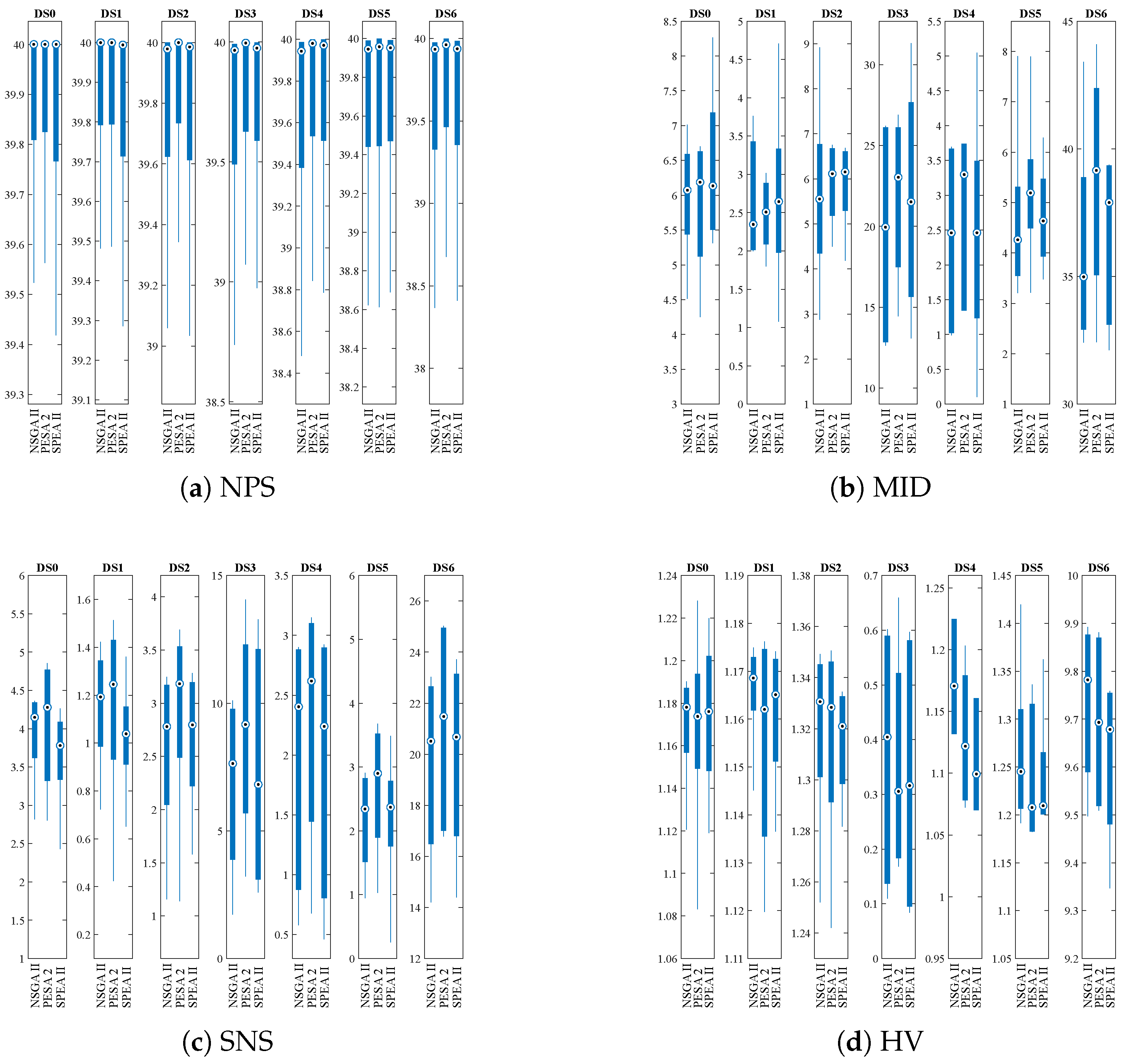
SPEA2	1.174	1.161	1.315	0.333	1.114	1.241	9.617

presents the mean values for each of the four performance measures on the Pareto fronts generated over the 200 independent runs on the seven sizes of the problem. Figure 2a–d present the corresponding box plots. Figure 2a shows that the median number of solutions in the Pareto fronts (NPS) is practically the same for all three algorithms. Figure 2b shows that for large instances the distance to the ideal solution (MID) is shorter for NSGA-II and SPEA2. The measure of the dispersion of non-dominated solutions on the Pareto front (SNS), shown in Figure 2c, yields, in general, better results with PESA-II than with NSGA-II and SPEA2. In terms of hypervolume (see Figure 2d), in large instances, NSGA-II shows a better performance than PESA-II and SPEA2.

Pairwise Tukey tests are performed to provide a statistical validation of the results. This test reduces the risk of incurring Type I errors. The hypotheses to be tested are as follows:

$$H_0:u_i-u_j=0 H_1:u_i-u_j\ne 0$$

where $u_i-u_j$ is the difference between the values of a pair of MOEAs under a given metric. The significance level $\left(\alpha \right)$ is set at 0.05.

Table 12. Statistical test results of MOEAs for the four criteria.

	NPS		MID		SNS		HV
DS0	$u_i-u_j$	$\mathit{p}$-value	$u_i-u_j$	$\mathit{p}$-value	$u_i-u_j$	$\mathit{p}$-value	$u_i-u_j$	$\mathit{p}$-value
NSGA-II vs. PESA-II	−0.038	0.025	0.131	0.026	−0.112	0.000	0.000	0.000
NSGA-II vs. SPEA2	0.007	0.502	−0.402	0.016	0.267	0.000	0.000	0.001
SPEA2 vs. PESA-II	−0.045	0.025	0.533	0.020	−0.379	0.000	0.004	0.002
DS1	$u_i-u_j$	$\mathit{p}$-value	$u_i-u_j$	$\mathit{p}$-value	$u_i-u_j$	$\mathit{p}$-value	$u_i-u_j$	$\mathit{p}$-value
NSGA-II vs. PESA-II	−0.006	0.628	0.212	0.019	−0.007	0.575	0.011	0.000
NSGA-II vs. SPEA2	0.026	0.056	−0.013	0.738	0.122	0.000	0.005	0.000
SPEA2 vs. PESA-II	−0.032	0.032	0.225	0.025	−0.129	0.000	0.007	0.000
DS2	$u_i-u_j$	$\mathit{p}$-value	$u_i-u_j$	$\mathit{p}$-value	$u_i-u_j$	$\mathit{p}$-value	$u_i-u_j$	$\mathit{p}$-value
NSGA-II vs. PESA-II	−0.062	0.025	−0.292	0.000	−0.380	0.000	0.004	0.002
NSGA-II vs. SPEA2	0.002	0.938	−0.282	0.000	0.109	0.000	0.005	0.000
SPEA2 vs. PESA-II	−0.063	0.025	−0.009	0.791	−0.279	0.000	0.000	0.000
DS3	$u_i-u_j$	$\mathit{p}$-value	$u_i-u_j$	$\mathit{p}$-value	$u_i-u_j$	$\mathit{p}$-value	$u_i-u_j$	$\mathit{p}$-value
NSGA-II vs. PESA-II	−0.083	0.025	−2.189	0.000	−2.135	0.000	0.017	0.051
NSGA-II vs. SPEA2	−0.037	0.085	−2.233	0.000	−0.636	0.000	0.038	0.000
SPEA2 vs. PESA-II	−0.046	0.034	0.044	0.858	−1.499	0.000	−0.020	0.015
DS4	$u_i-u_j$	$\mathit{p}$-value	$u_i-u_j$	$\mathit{p}$-value	$u_i-u_j$	$\mathit{p}$-value	$u_i-u_j$	$\mathit{p}$-value
NSGA-II vs. PESA-II	−0.092	0.025	−0.209	0.000	−0.299	0.000	0.048	0.000
NSGA-II vs. SPEA2	−0.057	0.037	−0.070	0.221	0.053	0.215	0.064	0.000
SPEA2 vs. PESA-II	−0.035	0.122	−0.139	0.015	−0.352	0.000	−0.010	0.000
DS5	$u_i-u_j$	$\mathit{p}$-value	$u_i-u_j$	$\mathit{p}$-value	$u_i-u_j$	$\mathit{p}$-value	$u_i-u_j$	$\mathit{p}$-value
NSGA-II vs. PESA-II	−0.027	0.286	−0.641	0.000	−0.528	0.000	0.023	0.000
NSGA-II vs. SPEA2	−0.010	0.702	−0.154	0.001	0.082	0.009	0.027	0.000
SPEA2 vs. PESA-II	−0.017	0.502	−0.487	0.000	−0.442	0.000	0.000	0.000
DS6	$u_i-u_j$	$\mathit{p}$-value	$u_i-u_j$	$\mathit{p}$-value	$u_i-u_j$	$\mathit{p}$-value	$u_i-u_j$	$\mathit{p}$-value
NSGA-II vs. PESA-II	−0.071	0.036	−2.622	0.000	−1.511	0.000	0.043	0.000
NSGA-II vs. SPEA2	−0.027	0.370	−0.463	0.001	0.350	0.016	0.120	0.000
SPEA2 vs. PESA-II	−0.044	0.131	−2.160	0.000	−1.162	0.000	−0.080	0.000

presents the results of the hypothesis tests. A p-value < $\alpha$ indicates that there is sufficient evidence to reject the null hypothesis; therefore, it can be concluded that significant differences are found between the means compared. Taking this into account, it can be seen that, for the NPS metric, in general, no significant differences are observed between NSGA-II and SPEA2; however, PESA-II obtains higher mean values. For the MID metric, in general, significant differences are observed between the algorithms, and, in particular, for large and medium-sized instances, NSGA-II obtains smaller mean values, followed by PESA-II. In general, significant differences between the algorithms are also observed for the SNS metric, with PESA-II obtaining higher mean values. Finally, significant differences are detected for the hypervolumes obtained by the three MOEAs in the different instances. Moreover, NSGA-II obtains the highest mean values.

These statistical tests validate the results presented in Table 11 and depicted in Figure 2a–d. In large instances, hybridized NSGA-II reaches Pareto fronts with mean hypervolumes up to 10% larger than those obtained by the other algorithms. The mean distances to the ideal solution are 17% shorter (averaging the large DS3 and DS6 instances) with NSGA-II. Finally, concerning the mean dispersion in the fronts, in the small and medium-sized instances, NSGA-II gives worse results than the other MOEAs but, in large instances, its results are similar or even better than those of the other two algorithms.

Figure 3a–d depict the fronts selected by TOPSIS (see

Table A1. TOPSIS DS2.

Ord.	S(v)	v1	v2
1°	0.583	0.318	0.516
2°	0.575	0.437	0.412
3°	0.572	0.401	0.454
4°	0.571	0.231	0.627
5°	0.571	0.267	0.591
6°	0.57	0.304	0.557
7°	0.568	0.217	0.646
8°	0.563	0.014	0.861
9°	0.563	0.515	0.359
10°	0.563	0.178	0.696
11°	0.563	0.387	0.488
12°	0.562	0.123	0.753
13°	0.56	0.139	0.74
14°	0.56	0.37	0.51
15°	0.559	0.295	0.587
16°	0.558	0.432	0.452
17°	0.558	0.103	0.781
18°	0.556	0.632	0.255
19°	0.555	0.579	0.311
20°	0.555	0.716	0.175
21°	0.551	0.66	0.238
22°	0.55	0.618	0.281
23°	0.547	0.05	0.856
24°	0.546	0.075	0.833
25°	0.542	0.682	0.234
26°	0.541	0.616	0.303
27°	0.54	0.699	0.22
28°	0.535	0.825	0.106
29°	0.534	0.763	0.169
30°	0.534	0.847	0.086
31°	0.531	0.786	0.152
32°	0.531	0.855	0.083
33°	0.531	0.816	0.122
34°	0.524	0.911	0.041
35°	0.517	0.942	0.024
36°	0.515	0.933	0.036
37°	0.506	0.908	0.08
38°	0.505	0.972	0.018
39°	0.5	0	1
40°	0.5	1	0

,

Table A2. TOPSIS DS3.

Ord.	S(v)	v1	v2
1°	0.608	0.322	0.463
2°	0.604	0.298	0.494
3°	0.599	0.391	0.412
4°	0.596	0.175	0.633
5°	0.596	0.282	0.527
6°	0.596	0.356	0.453
7°	0.591	0.273	0.545
8°	0.59	0.629	0.191
9°	0.59	0.254	0.566
10°	0.588	0.2	0.624
11°	0.588	0.475	0.349
12°	0.586	0.236	0.591
13°	0.585	0.546	0.283
14°	0.584	0.599	0.233
15°	0.581	0.613	0.224
16°	0.58	0.459	0.38
17°	0.58	0.448	0.392
18°	0.576	0.746	0.101
19°	0.575	0.706	0.145
20°	0.571	0.597	0.261
21°	0.569	0.534	0.327
22°	0.567	0.821	0.044
23°	0.564	0.126	0.746
24°	0.56	0.739	0.141
25°	0.56	0.161	0.719
26°	0.558	0.704	0.179
27°	0.556	0.144	0.744
28°	0.546	0.112	0.797
29°	0.545	0.121	0.789
30°	0.541	0.068	0.85
31°	0.54	0.032	0.888
32°	0.535	0.102	0.828
33°	0.535	0.065	0.865
34°	0.535	0.012	0.923
35°	0.532	0.031	0.913
36°	0.531	0.013	0.966
37°	0.525	0.021	0.963
38°	0.505	0.03	0.909
39°	0.5	0	1
40°	0.5	1	0

,

Table A3. TOPSIS DS5.

Ord.	S(v)	v1	v2
1°	0.577	0.358	0.488
2°	0.566	0.434	0.434
3°	0.563	0.297	0.578
4°	0.56	0.406	0.475
5°	0.553	0.557	0.338
6°	0.551	0.486	0.412
7°	0.546	0.509	0.399
8°	0.545	0.524	0.387
9°	0.545	0.604	0.307
10°	0.545	0.118	0.793
11°	0.539	0.236	0.686
12°	0.538	0.726	0.197
13°	0.538	0.656	0.269
14°	0.536	0.16	0.767
15°	0.534	0.821	0.112
16°	0.532	0.255	0.681
17°	0.529	0.75	0.192
18°	0.528	0.868	0.076
19°	0.527	0.703	0.244
20°	0.525	0.09	0.859
21°	0.525	0.901	0.05
22°	0.524	0.896	0.056
23°	0.522	0.925	0.031
24°	0.522	0.943	0.012
25°	0.521	0.939	0.019
26°	0.521	0.929	0.029
27°	0.519	0.807	0.155
28°	0.519	0.802	0.16
29°	0.518	0.104	0.859
30°	0.517	0.698	0.267
31°	0.517	0.778	0.187
32°	0.515	0.797	0.173
33°	0.508	0.972	0.012
34°	0.503	0.991	0.004
35°	0.501	0.061	0.953
36°	0.5	0.987	0.01
37°	0.5	0.07	0.94
38°	0.5	0.989	0.006
39°	0.5	0	1
40°	0.5	1	0

and

Table A4. TOPSIS DS6.

Ord.	S(v)	v1	v2
1°	0.765	0.29	0.179
2°	0.765	0.419	0.051
3°	0.757	0.439	0.047
4°	0.757	0.439	0.047
5°	0.756	0.255	0.234
6°	0.755	0.315	0.175
7°	0.754	0.382	0.109
8°	0.754	0.382	0.109
9°	0.747	0.248	0.258
10°	0.744	0.494	0.019
11°	0.744	0.494	0.019
12°	0.742	0.469	0.047
13°	0.737	0.481	0.045
14°	0.737	0.481	0.045
15°	0.734	0.519	0.014
16°	0.734	0.519	0.014
17°	0.732	0.372	0.165
18°	0.718	0.244	0.321
19°	0.705	0.173	0.416
20°	0.702	0.582	0.013
21°	0.697	0.6	0.007
22°	0.697	0.6	0.007
23°	0.685	0.234	0.396
24°	0.665	0.156	0.514
25°	0.662	0.669	0.006
26°	0.646	0.703	0.006
27°	0.644	0.152	0.559
28°	0.636	0.145	0.583
29°	0.634	0.142	0.591
30°	0.605	0.786	0.004
31°	0.605	0.786	0.004
32°	0.605	0.786	0.004
33°	0.597	0.042	0.763
34°	0.596	0.131	0.677
35°	0.594	0.127	0.685
36°	0.565	0.11	0.76
37°	0.509	0.039	0.943
38°	0.506	0.048	0.913
39°	0.5	1	0
40°	0.5	0	1

in the Appendix A).

The results obtained by TOPSIS are compared with those of the M1 single-objective model of Tsai et al. (2008) [2]. In this model, the authors consider the total operating cost (TOC) obtained from the weighted sum of the travel cost (TC) and the costs of anticipation and tardiness (ET) [2].

Table 13. MCDM performance and comparison with the benchmark [2].

	M1	TOPSIS		M1	TOPSIS		M1	TOPSIS
	TOC (Small)			TOC (Medium)			TOC (Large)
DS1	1092.60	1078.50	DS2	3104.83	2914.24	DS3	9207.13	8217.20
DS4	1322.20	1287.51	DS5	4431.03	4098.40	DS6	14,546.63	12,848.32

and

Table 14. Comparisons of mean criteria ratios.

	TOPSIS/M1		TOPSIS/M1		TOPSIS/M1
	Small		Medium		Large
DS1	0.987	DS2	0.939	DS3	0.892
DS4	0.974	DS5	0.925	DS6	0.883

compare the solutions of TOPSIS with the results obtained with the M1 model for instances DS1 to DS6 [2]. The columns in Table 13 show the TOC values in both cases, while the columns in Table 14 show the ratios between these values. It can be seen that the solutions of TOPSIS, in the smaller instances, do not differ much from those obtained by Tsai et al. (2008) [2] for the M1 model but, in larger instances, the solutions of TOPSIS are better in terms of TOC.

Figure 4 depicts these differences. It can be seen that the benchmark solutions are dominated by the best-ranked solution by TOPSIS on the front obtained by the hybridized NSGA-II algorithm.

7. Conclusions

This paper presents an integrated procedure to solve the joint OBP–OPP problem by combining an MOO and an MCDM. The first one consists of a MOEA that produces an approximate Pareto front. In the second one, TOPSIS is applied, which ranks the solutions of this approximate Pareto front according to their similarity ratios and selects the best one.

The objective of the procedure is the minimization of both the total operational cost of the pick-up process and the total earliness picking time. This multi-criteria approach considers the trade-off between minimization of operational costs and inefficiency due to earliness in the positioning of items to be included in the batches, assuming that no delays are allowed.

Three multiobjective hybrid evolutionary algorithms based on the dominance relation among solutions (NSGA-II, SPEA2, and PESA-II) are applied and compared on small, medium-sized, and large instances of mono and multilevel storage systems by Tsai et al. (2008) [2] Four performance metrics are used to compare the performance of the proposed multi-objective algorithms according to different measures: NPS, MID, SNS, and HV.

The results were statistically validated using Tukey’s test of difference of means for each of the metrics. It is found that on medium-sized and large instances, the hybridized NSGA-II algorithm achieves Pareto fronts with mean hypervolumes up to 10% above those of the other two algorithms, while the distances to the ideal solution are around 17% shorter, on average, for the large DS3 and DS6 instances. On the other hand, NSGA-II achieves a similar or even higher mean dispersion on large instances, although in smaller instances the other two MOEAs show better results.

In small-sized instances, TOPSIS does not yield better top-ranked results than those of the M1 model of Tsai et al. (2008) [2]. On the contrary, in large instances, the best-ranked results of the hybridized TOPSIS procedure proposed in this paper dominate those of the benchmark model.

Taking into account the growing importance of e-commerce and the high costs of picking activities in logistic centers, the proposed methodology can contribute to reducing those costs and gaining efficiency in their procedures.

Future work includes finding optimal placings for the articles, simultaneously taking into account aspects such as the size of the goods, the volume of their packaging, their relative demands, as well as operational considerations.

References

- Sancaklı, E.; Dumlupınar, İ.; Akçın, A.O.; Çınar, E.; Geylani, İ.; Düzgit, Z. Design of a Routing Algorithm for Efficient Order Picking in a Non-traditional Rectangular Warehouse Layout. In Proceedings of the Digitizing Production Systems, Online, 7–9 October 2021; Durakbasa, N.M., Gençyılmaz, M.G., Eds.; Springer: Cham, Switzerland, 2022; pp. 401–412. [Google Scholar]
- Tsai, C.Y.; Liou, J.; Huang, T.M. Using a multiple-GA method to solve the batch picking problem: Considering travel distance and order due time. Int. J. Prod. Res. 2008, 46, 6533–6555. [Google Scholar] [CrossRef]
- Miguel, F.; Frutos, M.; Tohmé, F.; Rossit, D.A. A memetic algorithm for the integral OBP/OPP problem in a logistics distribution center. Uncertain Supply Chain. Manag. 2019, 7, 203–214. [Google Scholar] [CrossRef]
- Miguel, F.M.; Frutos, M.; Méndez, M.; Tohmé, F. Solving Order Batching/Picking Problems with an Evolutionary Algorithm. In Proceedings of the International Conference of Production Research—Americas, Bahía Blanca, Argentina, 9–11 December 2020; Rossit, D.A., Tohmé, F., Mejía Delgadillo, G., Eds.; Communications in Computer and Information Science Series. Springer: Cham, Switzerland, 2021; pp. 177–186. [Google Scholar] [CrossRef]
- van Gils, T.; Ramaekers, K.; Braekers, K.; Depaire, B.; Caris, A. Increasing order picking efficiency by integrating storage, batching, zone picking, and routing policy decisions. Int. J. Prod. Econ. 2018, 197, 243–261. [Google Scholar] [CrossRef]
- de Koster, R.; Le-Duc, T.; Roodbergen, K.J. Design and control of warehouse order picking: A literature review. Eur. J. Oper. Res. 2007, 182, 481–501. [Google Scholar] [CrossRef]
- ten Hompel, M.; Schmidt, T. Warehouse Management; Springer: Berlin/Heidelberg, Germany, 2007. [Google Scholar] [CrossRef]
- de Koster, M.B.M.; van der Poort, E.; Wolters, M. Efficient orderbatching methods in warehouses. Int. J. Prod. Res. 1999, 37, 1479–1504. [Google Scholar] [CrossRef]
- Hofmann, F.M.; Visagie, S.E. The Effect of Order Batching on a Cyclical Order Picking System. In Proceedings of the International Conference on Computational Logistics, Enschede, The Netherlands, 27–29 September 2021; Mes, M., Lalla-Ruiz, E., Voß, S., Eds.; Lecture Notes in Computer Science. Springer: Cham, Switzerland, 2021; pp. 252–268. [Google Scholar] [CrossRef]
- Scholz, A.; Wäscher, G. Order Batching and Picker Routing in manual order picking systems: The benefits of integrated routing. Cent. Eur. J. Oper. Res. 2017, 25, 491–520. [Google Scholar] [CrossRef]
- Miguel, F.M.; Frutos, M.; Méndez, M.; Tohmé, F. Order batching and order picking with 3D positioning of the articles: Solution through a hybrid evolutionary algorithm. Math. Biosci. Eng. 2022, 19, 5546–5563. [Google Scholar] [CrossRef]
- Grosse, E.H.; Glock, C.H. The effect of worker learning on manual order picking processes. Int. J. Prod. Econ. 2015, 170, 882–890. [Google Scholar] [CrossRef]
- Žulj, I.; Glock, C.H.; Grosse, E.H.; Schneider, M. Picker routing and storage-assignment strategies for precedence-constrained order picking. Comput. Ind. Eng. 2018, 123, 338–347. [Google Scholar] [CrossRef]
- Chen, M.C.; Wu, H.P. An association-based clustering approach to order batching considering customer demand patterns. Omega 2005, 33, 333–343. [Google Scholar] [CrossRef]
- Henn, S.; Koch, S.; Wäscher, G. Order Batching in Order Picking Warehouses: A Survey of Solution Approaches. In Warehousing in the Global Supply Chain: Advanced Models, Tools and Applications for Storage Systems; Manzini, R., Ed.; Springer: London, UK, 2012; pp. 105–137. [Google Scholar] [CrossRef]
- Ardjmand, E.; Youssef, E.M.; Moyer, A.; Ii, W.A.Y.; Weckman, G.R.; Shakeri, H. A multi-objective model for minimising makespan and total travel time in put wall-based picking systems. Int. J. Logist. Syst. Manag. 2020, 36, 138–176. [Google Scholar] [CrossRef]
- Scholz, A.; Schubert, D.; Wäscher, G. Order picking with multiple pickers and due dates—Simultaneous solution of Order Batching, Batch Assignment and Sequencing, and Picker Routing Problems. Eur. J. Oper. Res. 2017, 263, 461–478. [Google Scholar] [CrossRef]
- Deb, K.; Pratap, A.; Agarwal, S.; Meyarivan, T. A fast and elitist multiobjective genetic algorithm: NSGA-II. IEEE Trans. Evol. Comput. 2002, 6, 182–197. [Google Scholar] [CrossRef]
- Zitzler, E.; Laumanns, M.; Thiele, L. SPEA2: Improving the Strength Pareto Evolutionary Algorithm; Technical Report; ETH: Zurich, Switzerland, 2001. [Google Scholar] [CrossRef]
- Corne, D.W.; Jerram, N.R.; Knowles, J.D.; Oates, M.J. PESA-II: Region-based selection in evolutionary multiobjective optimization. In Proceedings of the 3rd Annual Conference on Genetic and Evolutionary Computation, GECCO ’01, San Francisco, CA, USA, 7–11 July 2001; pp. 283–290. [Google Scholar]
- Hwang, C.L.; Yoon, K. Methods for Multiple Attribute Decision Making. In Multiple Attribute Decision Making: Methods and Applications A State-of-the-Art Survey; Hwang, C.L., Yoon, K., Eds.; Lecture Notes in Economics and Mathematical Systems; Springer: Berlin/Heidelberg, Germany, 1981; pp. 58–191. [Google Scholar] [CrossRef]
- Pardo, E.G.; Gil-Borrás, S.; Alonso-Ayuso, A.; Duarte, A. Order batching problems: Taxonomy and literature review. Eur. J. Oper. Res. 2023, 313, 1–24. [Google Scholar] [CrossRef]
- Henn, S.; Wäscher, G. Tabu search heuristics for the order batching problem in manual order picking systems. Eur. J. Oper. Res. 2012, 222, 484–494. [Google Scholar] [CrossRef]
- Rana, K. Order Picking in Narrow-Aisle Warehouses. Int. J. Phys. Distrib. Logist. Manag. 1990, 20, 9–15. [Google Scholar] [CrossRef]
- Hwang, H.; Kim, D.G. Order-batching heuristics based on cluster analysis in a low-level picker-to-part warehousing system. Int. J. Prod. Res. 2005, 43, 3657–3670. [Google Scholar] [CrossRef]
- Olmos, J.; Florencia, R.; García, V.; González, M.V.; Rivera, G.; Sánchez-Solís, P. Metaheuristics for Order Picking Optimisation: A Comparison Among Three Swarm-Intelligence Algorithms. In Technological and Industrial Applications Associated with Industry 4.0; Ochoa-Zezzatti, A., Oliva, D., Hassanien, A.E., Eds.; Studies in Systems, Decision and Control; Springer International Publishing: Cham, Switzerland, 2022; pp. 177–194. [Google Scholar] [CrossRef]
- Ardjmand, E.; Shakeri, H.; Singh, M.; Sanei Bajgiran, O. Minimizing order picking makespan with multiple pickers in a wave picking warehouse. Int. J. Prod. Econ. 2018, 206, 169–183. [Google Scholar] [CrossRef]
- Masae, M.; Glock, C.H.; Grosse, E.H. Order picker routing in warehouses: A systematic literature review. Int. J. Prod. Econ. 2020, 224, 107564. [Google Scholar] [CrossRef]
- Cergibozan, C.; Tasan, A.S. Order batching operations: An overview of classification, solution techniques, and future research. J. Intell. Manuf. 2019, 30, 335–349. [Google Scholar] [CrossRef]
- Ho, Y.C.; Tseng, Y.Y. A study on order-batching methods of order-picking in a distribution centre with two cross-aisles. Int. J. Prod. Res. 2006, 44, 3391–3417. [Google Scholar] [CrossRef]
- Henn, S.; Schmid, V. Metaheuristics for order batching and sequencing in manual order picking systems. Comput. Ind. Eng. 2013, 66, 338–351. [Google Scholar] [CrossRef]
- Lam, C.H.; Choy, K.; Ho, G.; Lee, C. An order-picking operations system for managing the batching activities in a warehouse. Int. J. Syst. Sci. 2014, 45, 1283–1295. [Google Scholar] [CrossRef]
- van Gils, T.; Ramaekers, K.; Caris, A.; de Koster, R.B.M. Designing efficient order picking systems by combining planning problems: State-of-the-art classification and review. Eur. J. Oper. Res. 2018, 267, 1–15. [Google Scholar] [CrossRef]
- Petersen, C.G. An evaluation of order picking routeing policies. Int. J. Oper. Prod. Manag. 1997, 17, 1098–1111. [Google Scholar] [CrossRef]
- Theys, C.; Bräysy, O.; Dullaert, W.; Raa, B. Using a TSP heuristic for routing order pickers in warehouses. Eur. J. Oper. Res. 2010, 200, 755–763. [Google Scholar] [CrossRef]
- Henn, S.; Koch, S.; Doerner, K.F.; Strauss, C.; Wäscher, G. Metaheuristics for the Order Batching Problem in Manual Order Picking Systems. Bus. Res. 2010, 3, 82–105. [Google Scholar] [CrossRef]
- Chen, R.C.; Lin, C.Y. An efficient two-stage method for solving the order-picking problem. J. Supercomput. 2020, 76, 6258–6279. [Google Scholar] [CrossRef]
- Lu, W.; McFarlane, D.; Giannikas, V.; Zhang, Q. An algorithm for dynamic order-picking in warehouse operations. Eur. J. Oper. Res. 2016, 248, 107–122. [Google Scholar] [CrossRef]
- Diefenbach, H.; Emde, S.; Glock, C.H.; Grosse, E.H. New solution procedures for the order picker routing problem in U-shaped pick areas with a movable depot. OR Spectr. 2022, 44, 535–573. [Google Scholar] [CrossRef]
- Molnar, B.; Lipovszki, G. Multi-objective routing and scheduling of order pickers in a warehouse. Int. J. Simul. 2005, 6, 22–32. [Google Scholar]
- Pan, J.C.H.; Shih, P.H.; Wu, M.H. Storage assignment problem with travel distance and blocking considerations for a picker-to-part order picking system. Comput. Ind. Eng. 2012, 62, 527–535. [Google Scholar] [CrossRef]
- Battini, D.; Glock, C.H.; Grosse, E.H.; Persona, A.; Sgarbossa, F. Human energy expenditure in order picking storage assignment: A bi-objective method. Comput. Ind. Eng. 2016, 94, 147–157. [Google Scholar] [CrossRef]
- Elbert, R.M.; Franzke, T.; Glock, C.H.; Grosse, E.H. The effects of human behavior on the efficiency of routing policies in order picking: The case of route deviations. Comput. Ind. Eng. 2017, 111, 537–551. [Google Scholar] [CrossRef]
- Vazquez-Noguerol, M.; Comesaña-Benavides, J.A.; Riveiro-Sanroman, S.; Prado-Prado, J.C. A mixed integer linear programming model to support e-fulfillment strategies in warehouse-based supermarket chains. Cent. Eur. J. Oper. Res. 2022, 30, 1369–1402. [Google Scholar] [CrossRef]
- Kocaman, Y.; Öztürkoğlu, Ö.; Gümüşoğlu, Ş. Aisle designs in unit-load warehouses with different flow policies of multiple pickup and deposit points. Cent. Eur. J. Oper. Res. 2021, 29, 323–355. [Google Scholar] [CrossRef]
- Ardjmand, E.; Singh, M.; Shakeri, H.; Tavasoli, A.; Young II, W.A. Mitigating the risk of infection spread in manual order picking operations: A multi-objective approach. Appl. Soft Comput. 2021, 100, 106–953. [Google Scholar] [CrossRef] [PubMed]
- Zhang, M.; Grosse, E.H.; Glock, C.H. Ergonomic and economic evaluation of a collaborative hybrid order picking system. Int. J. Prod. Econ. 2023, 258, 108774. [Google Scholar] [CrossRef]
- Cano, J.A.; Correa-Espinal, A.A.; Gómez-Montoya, R.A. Mathematical programming modeling for joint order batching, sequencing and picker routing problems in manual order picking systems. J. King Saud Univ. Eng. Sci. 2020, 32, 219–228. [Google Scholar] [CrossRef]
- Cals, B.; Zhang, Y.; Dijkman, R.; van Dorst, C. Solving the online batching problem using deep reinforcement learning. Comput. Ind. Eng. 2021, 156, 107221. [Google Scholar] [CrossRef]
- Roodbergen, K.J.; de Koster, R. Routing order pickers in a warehouse with a middle aisle. Eur. J. Oper. Res. 2001, 133, 32–43. [Google Scholar] [CrossRef]
- Coello Coello, C. Evolutionary multi-objective optimization: A historical view of the field. IEEE Comput. Intell. Mag. 2006, 1, 28–36. [Google Scholar] [CrossRef]
- Srinivas, N.; Deb, K. Muiltiobjective Optimization Using Nondominated Sorting in Genetic Algorithms. Evol. Comput. 1994, 2, 221–248. [Google Scholar] [CrossRef]
- Deb, K.; Agrawal, S.; Pratap, A.; Meyarivan, T. A Fast Elitist Non-dominated Sorting Genetic Algorithm for Multi-objective Optimization: NSGA-II. In Proceedings of the Parallel Problem Solving from Nature PPSN VI, Paris, France, 18–20 September 2000; Schoenauer, M., Deb, K., Rudolph, G., Yao, X., Lutton, E., Merelo, J.J., Schwefel, H.P., Eds.; Lecture Notes in Computer Science. Springer: Berlin/Heidelberg, Germany, 2000; pp. 849–858. [Google Scholar] [CrossRef]
- Corne, D.W.; Knowles, J.D.; Oates, M.J. The Pareto Envelope-Based Selection Algorithm for Multiobjective Optimization. In Proceedings of the Parallel Problem Solving from Nature PPSN VI, Paris, France, 18–20 September 2000; Schoenauer, M., Deb, K., Rudolph, G., Yao, X., Lutton, E., Merelo, J.J., Schwefel, H.P., Eds.; Lecture Notes in Computer Science. Springer: Berlin/Heidelberg, Germany, 2000; pp. 839–848. [Google Scholar] [CrossRef]
- Zitzler, E. Evolutionary Algorithms for Multiobjective Optimization: Methods and Applications. Ph.D. Thesis, ETH Zurich, Zurich, Switzerland, 1999. [Google Scholar] [CrossRef]
- Dasarathy, B.V. Smart: Similarity measure anchored ranking technique for the analysis of multidimensional data arrays. IEEE Trans. Syst. Man, Cybern. 1976, 6, 708–711. [Google Scholar]
- Pomerol, J.C.; Barba-Romero, S. Multicriterion Decision in Management: Principles and Practice; International Series in Operations Research & Management Science; Springer: Boston, MA, USA, 2000. [Google Scholar] [CrossRef]
- Méndez, M.; Frutos, M.; Miguel, F.; Aguasca-Colomo, R. TOPSIS Decision on Approximate Pareto Fronts by Using Evolutionary Algorithms: Application to an Engineering Design Problem. Mathematics 2020, 8, 2072. [Google Scholar] [CrossRef]
- Lee, I.G.; Chung, S.H.; Yoon, S.W. Two-stage storage assignment to minimize travel time and congestion for warehouse order picking operations. Comput. Ind. Eng. 1976, 139, 106–129. [Google Scholar] [CrossRef]
- Karimi, N.; Zandieh, M.; Karamooz, H.R. Bi-objective group scheduling in hybrid flexible flowshop: A multi-phase approach. Expert Syst. Appl. 2010, 37, 4024–4032. [Google Scholar] [CrossRef]
- Holland, J.H. Adaptation in Natural and Artificial Systems; University of Michigan Press: Ann Arbor, MI, USA, 1975; Volume 7, pp. 390–401. [Google Scholar]
- Whitley, D.; Starkweather, T.; Fuquay, D. Scheduling problems and traveling salesman: The genetic edge recombination. In Proceedings of the Third International Conference on Genetic Algorithms, San Francisco, CA, USA, 4–7 June 1989; pp. 133–140. [Google Scholar]
- Wetzel, A. Evaluation of the Effectiveness of Genetic Algorithms in Combinatorial Optimization; University of Pittsburgh: Pittsburgh, PA, USA, 1983; Volume 1, pp. 1932–4537. [Google Scholar]
Figure 1.
Illustrations of a small layout representation with a position marker for a particular batch. (a) Orders batch (highlighted) in warehouse layout. (b) A graph-based representation of the underlying topology. (c) A picking tour for a particular batch of orders.
Figure 2.
Box-plots of measurement comparisons.
Figure 3.
Non-dominated solutions medium and large problem size.
Figure 4.
Comparison of the TOPSIS-based results with M1 in all instances.