Bidirectional Tracking Method for Construction Workers in Dealing with Identity Errors

Abstract

Online multi-object tracking (MOT) techniques are instrumental in monitoring workers’ positions and identities in construction settings. Traditional approaches, which employ deep neural networks (DNNs) for detection followed by body similarity matching, often overlook the significance of clear head features and stable head motions. This study presents a novel bidirectional tracking method that integrates intra-frame processing, which combines head and body analysis to minimize false positives and inter-frame matching to control ID assignment. By leveraging head information for enhanced body tracking, the method generates smoother trajectories with reduced ID errors. The proposed method achieved a state-of-the-art (SOTA) performance, with a multiple-object tracking accuracy (MOTA) of 95.191%, higher-order tracking accuracy (HOTA) of 78.884% and an identity switch (IDSW) count of 0, making it a strong baseline for future research.

1. Introduction

The efficacy of worker tracking in construction safety management, both on-site [1] and off-site [2], has been widely acknowledged. The real-time monitoring of workers’ locations and identities enables managers to monitor working conditions closely, facilitating prompt interventions to prevent potential accidents [3], such as ensuring helmet usage, maintaining safe distances and avoiding collisions with vehicles [4]. By analyzing tracking data, valuable insights can be derived into workers’ productivity, intensity, movement patterns and other critical aspects, ultimately optimizing construction processes and labor allocation, enhancing efficiency, minimizing resource waste and reducing labor-intensive tasks for workers [5].

Nonetheless, complex construction scenarios pose challenges in feature extraction and identity matching, leading to identity-tracking errors. Four types of errors are illustrated in Figure 1: identity missing, identity increase, identity switch (IDSW) and identity transfer (IDTR) [6]. Identity missing occurs when false negatives (FNs) in deep learning models result in missed identifications, as demonstrated by worker ID = 2 in Figure 1a, who was occluded by “Bar shop” in frame #78. Identity increase is due to false positives (FPs), as exemplified by worker ID = 7 in Figure 1b, where an incorrect bounding box detection led to an additional ID. IDSW refers to a single person being assigned different IDs consecutively, as in Figure 1c, where worker ID = 5 had different IDs in frames #99 and #130. Conversely, IDTR occurs when two individuals are mistakenly assigned the same ID, as shown in Figure 1d, where worker ID = 3 switched to ID = 4 between frames #140 and #259. Both IDTR and IDSW stem from issues with association algorithms, which can be interpreted as “accepting false ID” and “rejecting truth ID”.

Current MOT methods have some intrinsic limitations:

(1) Relying on detection DNNs [7] limits the number of tracked individuals to the detected count per frame. Missed detections lead to a lost person’s re-identification (ReID) [8] information and, subsequently, motion estimation for the corresponding sequence, resulting in tracking ID loss.

(2) Current motion estimation techniques are confined to the Kalman filter (KF) [9], which may not converge mathematically. In cases of divergence, the KF’s estimates become meaningless and can cause incorrect motion predictions.

(3) Worker tracking, unlike pedestrian tracking, encounters more occlusion challenges in complex scenarios [10], posing higher ID error risks. While pedestrian tracking algorithms typically overlook ID-related metrics, worker tracking, which is crucial for safety management, necessitates their consideration, particularly in MOT challenge-like contexts [11,12].

(4) Head information, which is vital for worker identification, has often been overlooked [2]. Its use is pivotal due to workers’ upright posture and less obstructed heads, which can enhance whole-body tracking by leveraging bidirectional matching algorithms. Head tracking, as it aids in body detection and tracking, exploits this relationship to improve robustness.

The main innovation of this article is to provide a simple bidirectional method for tracking workers under complex construction scenarios. This bidirectional interaction improves the accuracy and robustness of body tracking while also addressing issues such as occlusion and environmental changes. The proposed method can significantly improve the safety and efficiency of construction sites by enabling the tracking of worker positions and movements with fewer ID errors.

The contributions of this research are as follows:

(1) Adopting head-tracking-to-body-tracking models in the construction field for the first time and using head motion state to correct whole-body movement.

(2) In the case where KF cannot be abandoned for movement estimation, modifying the body speed into head speed and making it comply with the basic “near-big, far-small” perspective principle.

(3) Changing the unidirectional method to bidirectional and letting tracking outputs correct current frame detections.

(4) Demonstrating the effectiveness of this method from a mathematical perspective.

2. Related Works

Vision-based MOT methods aim to identify target IDs (humans, vehicles, etc.) across successive frames. MOT usually consists of three subtasks [13]: object detection, feature extraction and data association.

• Object detection (observation model): using a DNN such as Faster R-CNN [14], YOLO [15], CenterNet [16], or Transformer [17] to obtain the region of interest (ROI) [18], also called the bounding box.
• Feature extraction (appearance model): employing a person re-identification (ReID) [8] network to extract a unidimensional vector from the ROI.
• Data association (motion estimation and linear assignment): matching the IDs [7] between the targets detected by the DNN at the current frame and estimated using the KF at the former frame and the similarity cost matrix with Hungarian [19] or Jonker–Volgenant [7] algorithms.

According to the literature [2], instance segmentation has been posited to enhance detection performance, as exemplified by Xiao et al.’s [2] adaptation of the Mask R-CNN [20] for worker tracking. However, their study relies on datasets without annotations for heavily occluded individuals (occlusion rate above 70%), which precludes the possibility of improving the data association process, as previously noted by [10].

There are two basic paradigms for MOT [21]: tracking by detection (TBD) and joint detection and tracking (JDT).

• TBD treats object detection as a separate detector, while feature extraction and data association are considered trackers [8]. TBD offers the advantage of flexibility in replacing modules with better DNNs or association methods. However, the detector and the tracker cannot enhance each other’s performance. If the detector produces missing or false bounding boxes, this will result in the tracker’s failure to track or accurately identify the target.
• JDT integrates the detector and tracker into one unified network that can be trained end-to-end, such as Siamese [22] or Transformer networks [23]. JDT relies exclusively on appearance features, but the training of DNNs often demands better GPUs and takes significant time. For instance, TransTrack [24] demands 16.1 GB of GPU memory for inference, making it incompatible with the NVIDIA Tesla T4 (15 GB) on Google Colaboratory [25]. To provide a simple and training-free tracking method, TBD is the better choice.

Matching algorithms in TBD use various cues, including motion information [9], appearance features [26], velocity direction, confidence and height state [27], to calculate the different similarity distances (the cosine distance, the squared Mahalanobis distance, the intersection over union (IoU) distance, etc.) for the cost matrix in the linear assignment problem.

However, unlike pedestrian tracking on roads, the motion of workers always features long stays or frequent crossings [28], which may lead to the continuous growth of the covariance matrix in KF. In practical scenarios, a large covariance matrix can lead to the acceptance of false IDs. Conversely, a small covariance matrix can result in the rejection of the true ID. Hence, it is essential to carefully consider the covariance matrix size to ensure accurate identification. Convergence failure of the covariance matrix implies a mismatch between the selected motion model of the KF and actual motion behavior, but it does not seem to offer an alternative solution for the linear estimator [9].

To provide a comprehensive overview of data association techniques in the MOT domain, we present the technical aspects in

Table 1. Strengths and limitations of SOTA methods.

No.	SOTA Methods	Year	Information Types	Advantages (A) & Shortcomings (S)
1	SORT [19]	2016	O: Faster R-CNN; A: None; M: KF + IoU + Hungarian.	A: presented as the baseline; KF state is $x_t={\left[x_c,y_c,s,r,v_x,v_y,v_s\right]}^T$, s = aspect ratio and r = area. S: highly dependent on detection performance and many IDSWs; no occlusion-solving considerations.
2	DeepSORT [8]	2017	O: Faster R-CNN; A: ReID (128-d); M: KF + Cosine distance + IoU + Hungarian.	A: presented as the baseline integrate appearance information. KF state is $x_t={\left[x_c,y_c,\gamma ,h,v_x,v_y,v_{\gamma },v_h\right]}^T$, γ = aspect ratio and h = height. S: detection performance dependency; occlusion-related IDSWs reduced but still frequent; constant-velocity model.
3	ByteTrack [7]	2022	O: re-trained YOLOX-x on 1400 videos; A: ReID (1024-d); M: KF + Cosine distance + IoU + Hungarian + low scores re-match.	A: best performance in MOT20 and with already published codes. KF state is $x_t={\left[x_c,y_c,a,h,v_x,v_y,v_a,v_h\right]}^T$; a = aspect ratio and h = height. S: highly dependent on detection performance and many IDSWs; no occlusion considerations; constant-velocity model.
4	OC_SORT [9]	2022	O: baseline detections in MOTChallenge; A: None; M: KF + IoU + Hungarian + re-update of KF + motion direction difference.	A: first to explain the KF predict errors accumulation in detail; motion direction difference is added in the association cost matrix. KF state is $x_t={\left[x_c,y_c,a,s,v_x,v_y,v_a\right]}^T$, a = area and s = aspect ratio. S: no real online method for KF update; needs future frame; constant-velocity assumption during occlusion, cannot remain effective during long-term occlusions; detection performance dependency; constant-velocity model.
5	Deep OC_SORT [26]	2023	O: YOLOX; A: ReID (SBS50, 287MB) + Camera Motion Compensation + Dynamic Appearance; M: KF + IoU + Hungarian + re-update of KF + motion direction difference.	A: Apply Camera Motion Compensation to correct the KF state for better locations of the bounding box; apply detection confidence to modify ReID output vectors. KF state is $x_t={\left[x_c,y_c,a,s,v_x,v_y,v_a\right]}^T$; a = area and s = aspect ratio. S: the same as the OC_SORT; constant-velocity model.
6	BoTSORT [29]	2022	O: Faster R-CNN; A: ReID + Camera Motion Compensation; M: KF + cosine distance + IoU + Hungarian.	A: modify KF state to $x_t={\left[x_c,y_c,s,a,v_x,v_y,v_s\right]}^T$, s = area and a = aspect ratio; apply Camera Motion Compensation to reduce errors of moving cameras; apply new cost matrix with weights of appearance cost and motion cost. S: the same as the OC_SORT; constant-velocity model; slow when working with sparse optical flow.
7	Strong_SORT [30]	2022	O: YOLOX-x; A: ReID (BoT) + Camera Motion Compensation; M: NSA-KF + cosine distance + IoU + Hungarian.	A: apply a new cost matrix with weights of appearance cost and motion cost; KF state is $x_t={\left[x_c,y_c,a,h,v_x,v_y,v_a,v_h\right]}^T$; a = aspect ratio and h = height. S: MOTA is slightly lower, mainly due to the high detection score threshold leading to many missing detections; working speed is not high.
8	TransTrack [24]	2020	O: re-trained transformer; A: None; M: None.	A: Self-Attention Mechanism and Query-Key pipeline. S: hard to train; no motion information utilization; JDT not better than TBD in performance.
9	UniTrack [31]	2021	O: ResNet-50; A: ImageNet-supervised appearance model; M: KF + cosine distance + IoU + Hungarian.	A: can support different tracking tasks and leverage many existing general appearance models. KF state is $x_t={\left[x_c,y_c,a,h,v_x,v_y,v_a,v_h\right]}^T$; a = aspect ratio and h = height. S: not better in terms of metrics performance.
10	FairMOT [32]	2020	O: encoder–decoder; A: encoder–decoder; M: KF + cosine distance + IoU + Hungarian.	A: one encoder–decoder network to obtain observation and appearance at the same time, with no need for an independent ReID model; S: need training for about 30 h on two RTX 2080 Ti GPUs; still a SORT-related method.
11	TransMOT [33]	2021	O: spatial–temporal graph Transformer; A: None; M: KF + cosine distance + IoU + Hungarian.	A: A cascaded association structure to handle low confidence detection and long-term occlusion. S: relatively large computing resources and data; no public codes.
12	Hybrid-SORT [27]	2023	O: YOLOX-x; A: ReID + Camera Motion Compensation; M: KF + cosine distance + IoU + Hungarian + weak cues.	A: apply a new cost matrix with weights of appearance cost, motion cost, four corners’ velocity direction, and height-modulated IoU. KF state is $x_t={\left[x_c,y_c,s,c,r,v_x,v_y,v_s,v_c\right]}^T$; r = aspect ratio, s = area and c = confidence score. S: detection performance dependency.
13	Xiao et al. [2]	2023	O: Mask R-CNN; A: ReID (128-d); M: KF + cosine distance + IoU + Hungarian.	A: baseline in worker tracking; S: needs retraining on a new dataset; does not address severe occlusions; no public codes.

Observation DNN: O; appearance DNN: A; motion estimation model and assignment algorithm: M.

. Contemporary methods focus on retraining detection DNNs for improved input accuracy, while others refine Kalman filter state vectors. Given our emphasis on data association, object detection and feature extraction details are not elaborated upon in this section.

The SOTA tracking-by-detection methods, as depicted in Table 1, are unidirectional, relying solely on the outputs of detection DNNs. Consequently, their tracking capacity is inherently limited to the number of detected objects, and the tracking ID count never exceeds the detection ID count. Our proposed bidirectional tracking approach encompasses two types of interactions, namely, head-to-body and detector–tracker, which enable the mutual correction of tracking and detection results, enhancing the overall performance.

3. Motion Estimation with KF

3.1. Basic KF Formula

Motion data, including position and velocity, can be effectively extracted using a linear Kalman filter (KF) [10]. The KF estimates the state of a dynamic system from noisy measurements, employing a state equation and an observation equation, as depicted in Equations (1) and (2).

In Equation (1), the prior state vector estimate (denoted by ${\overline{x}}_t$) is predicted based on the posterior distribution from the previous frame (denoted by ${\widehat{x}}_{t-1}$). The state vector $x_t={\left[x_c,y_c,a,h,v_x,v_y,v_a,v_h\right]}^T$ is (8 × 1) in frame t and consists of the bounding box center, with dimensions, width, height, $a=w/h$ and velocity. The transition matrix F_t governs the system dynamics, while Q_t (8 × 8) represents process noise, following a normal distribution.

$${\overline{x}}_t=F_t{\widehat{x}}_{t-1}+{\omega }_t,{\omega }_t\sim N\left(0,Q_t\right)$$

(1)

Equation (2) accounts for imperfect estimation, where the measurement $z_{t-1}={\left[x_c,y_c,a,h\right]}^T$ (a 4 × 1 vector in frame t − 1) and the projected posterior distribution are subject to observation noise (denoted by R_t, a 4 × 4 matrix). The observation matrix H facilitates dimensional transformation between state and measurement vectors.

$$z_{t-1}=H_t{\overline{x}}_{t-1}+{\nu }_t,{\nu }_t\sim N\left(0,R_t\right)$$

(2)

The KF’s prediction for the covariance matrix P_t is shown in Equation (3). Since elements in the vector can vary widely, a covariance matrix is used to quantify the variation between elements. P_t (8 × 8) is updated regardless of the presence of a tracking ID, with a “dummy update” [9] occurring during tracking, which can lead to error accumulation and non-convergence.

$${\overline{P}}_t=F_t{\widehat{P}}_{t-1}{F}_t^{\top }+Q_t$$

(3)

The Kalman gain, denoted in Equation (4), determines the influence of the current observation on state estimation. A higher value of $K_t$ indicates greater confidence in the detection, while a lower value suggests a greater confidence in the prediction. Elements of $K_t$(an 8 × 4 matrix) are confined to the range [0, 1] during normal operation.

$$K_t=\frac{{\overline{P}}_t{H}_t^{\top }}{\left(H_t{\overline{P}}_t{H}_t^{\top }+R_t\right)}={\widehat{P}}_t{H}_t^{\top }{R_t}^{-1}$$

(4)

Finally, Equations (5) and (6) describe the posterior update of the state vector and covariance matrix, respectively, incorporating the prior estimate and current observation data.

$${\widehat{x}}_t={\overline{x}}_t+K_t\left(z_t-H_t{\overline{x}}_t\right)=F_t{\widehat{x}}_{t-1}+K_t\left(z_t-H_t{F}_t{\widehat{x}}_{t-1}\right)$$

(5)

$${\widehat{P}}_t=\left(I-K_t{H}_t\right){\overline{P}}_t$$

(6)

3.2. KF Divergence Proof

This section elucidates the mechanism behind the non-convergence of the covariance matrix in the KF. When the employed motion estimation model in the KF mismatches the actual dynamics, iterative updates lead to divergence. Given the practical challenge of acquiring a precise motion model for humans, the KF often encounters the following issue:

• If the KF divergence → elements in the covariance matrix $P_t$ is larger → elements in the inverse covariance matrix ${P_t}^{-1}$ is smaller → Mahalanobis distance of two different persons’ IDs is smaller than the threshold → leading to “accepting false ID” errors

Consequently, addressing the KF divergence problem is crucial for reducing such identity errors. From the perspective of Bayesian probabilities, (1) can be expressed as $p\left(\overline{x_t}\right)=N\left(\mu ,\overline{P_t}\right)$, and if $\overline{x_t}$ is given, (2) can be expressed as $p\left(z_t\left|\overline{x_t}\right.\right)=N\left(H_t\mu ,R\right)$; then, $p\left(\widehat{x_t}\left|z_t\right.\right)=p\left(z_t\left|\overline{x_t}\right.\right)\times p\left(\overline{x_t}\right)$, so the corresponding equation of the covariance matrix is as described as follows (7):

$${\widehat{P_t}}^{-1}={H_t}^T{R}^{-1}{H}_t+{\overline{P_t}}^{-1}$$

(7)

Assuming a simple constant-velocity model, the ground truth motion yields (8):

$$\begin{array}{l}{x_t}^{*}={x_{t-1}}^{*}+v^{*}={x_0}^{*}+t{v}^{*}\\ {z_t}^{*}={x_t}^{*}+{\epsilon }_t={x_0}^{*}+t{v}^{*}+{\epsilon }_t\end{array}$$

(8)

Assuming the estimation model is not the same as the ground truth yields (9):

$$\begin{array}{l}{x}_t=x_{t-1}+v=x_0+tv,v\ne v^{*}\& x_0={x_0}^{*}\\ z_t=x_t+{\epsilon }_t=x_0+tv+{\epsilon }_t\end{array}$$

(9)

For one element p_t in the covariance matrix, assuming there is no relevant prior knowledge of noise and initial value at t = 0, let $r_0={\sigma }^2,p_0=\infty$. For the constant-velocity model, $f_t=h_t=1$, the following is obtained (10):

$$\begin{array}{l}{p_t}^{-1}={\left[f_t{p}_{t-1}{f}_t^T\right]}^{-1}+{\left[h_{t}r{h}_t^T\right]}^{-1}=\left[{p_{t-1}}^{-1}\right]+\left[{\sigma }^{-2}\right]\\ =\left(\left[{p_{t-2}}^{-1}\right]+\left[{\sigma }^{-2}\right]\right)+\left[{\sigma }^{-2}\right]\\ \dots \\ =\left[{p_0}^{-1}\right]+t\times \left[{\sigma }^{-2}\right]\\ =\frac{1}{\infty }+\frac{t}{{\sigma }^2}=\frac{t}{{\sigma }^2}\end{array}$$

(10)

(4) can be rewritten in one element of the vector, which yields (11):

$$k_t={\widehat{p}}_t{h}_t^{\top }{r_t}^{-1}=\frac{{\sigma }^2}{t}\frac{1}{{\sigma }^2}=\frac{1}{t}$$

(11)

Substituting (2) into (5) as one element of the posterior state vector yields (12):

$$\begin{array}{l}{\widehat{x}}_t=f_t{\widehat{x}}_{t-1}+k_t\left(z_t-h_t{f}_t{\widehat{x}}_{t-1}\right)=({\widehat{x}}_{t-1}+v)+\frac{1}{t}\left(z_t-{\widehat{x}}_{t-1}-v\right)\\ =\frac{t-1}{t}\left({\widehat{x}}_{t-1}+v\right)+\frac{1}{t}{z}_t\\ =\left(\underset{\to 0}{\underbrace{\frac{t-2}{t}}}\left({\widehat{x}}_{t-2}+v\right)+\frac{1}{t}{z}_{t-1}\right)+\frac{1}{t}{z}_t\\ \dots \\ =\frac{1}{t}\left(z_1+z_2+z_3+\dots +z_t\right)\\ =\frac{1}{t}\left(x_0+v+{\epsilon }_1\right)+\frac{1}{t}\left(x_0+2v+{\epsilon }_2\right)+\dots +\frac{1}{t}\left(x_0+tv+{\epsilon }_t\right)\\ =x_0+\frac{1}{t}\frac{(1+t)\ast t}{2}(v+\epsilon )=x_0+\frac{(t+1)}{2}v+\frac{1}{t}{\displaystyle \sum _{i=1}^t{\epsilon }_i}\end{array}$$

(12)

Under the constant-velocity assumption, the discrepancy between the ground truth and posterior estimates (13) exhibits an increasing trend with time. This observation implies that the error grows over time, leading to the divergence of the KF under constant perturbations. Consequently, when the employed motion estimation model deviates from the true dynamics, KF performance is significantly compromised, as it is prone to divergence issues. Given the complexity of worker movements, current research efforts, as exemplified by [7], have not been able to establish accurate motion models, resulting in the persistent challenge of mitigating KF divergence still needing a reasonable mathematical solution. Therefore, it is necessary to find ways to bypass the divergence problem.

$$\begin{array}{l}\Delta ={x_t}^{*}-{\widehat{x}}_t={x_0}^{*}+t{v}^{*}-x_0-\frac{(1+t)}{2}v-\frac{1}{t}{\displaystyle \sum _{i=1}^t{\epsilon }_i}=\frac{t-1}{2}(v^{*}-v)-\frac{1}{t}{\displaystyle \sum _{i=1}^t{\epsilon }_i}\\ E\left(\Delta \right)=\frac{t-1}{2}(v^{*}-v)\\ D\left(\Delta \right)={\left(\frac{t-1}{2}(v^{*}-v)\right)}^2+\frac{{\sigma }^2}{t}\end{array}$$

(13)

3.3. KF Processing Example

In this section, we demonstrate that despite the inherent limitations of the KF’s motion estimation, achieving convergence can still be accomplished through continuous and accurate detection measurements.

The state equation initialization requires understanding the motion model of the object, such as the uniformly moving, two-dimensional object in (14). On occasions where there was no fixed frame interval time in videos, $\Delta t$ was assigned the value 1.0, and could be adjusted through velocity.

$$\begin{array}{l}{x}_t=x_{t-1}+v_{t-1}^x\times \Delta t\\ y_t=y_{t-1}+v_{t-1}^y\times \Delta t\\ v_{t-1}^x=v_{t-1}^x\\ v_{t-1}^y=v_{t-1}^y\end{array}$$

(14)

Similar to (14), Equation (1), rewritten into the matrix form, can be presented as (15). At this point, our estimation motion model will be fixed.

$$\overrightarrow{x_t}=\left(\begin{array}{l}{x}_t\\ y_t\\ a_t\\ h_t\\ v_t^x\\ v_t^y\\ v_t^a\\ v_t^h\end{array}\right)=\left[\begin{array}{cccccccc}1& 0& 0& 0& 1& 0& 0& 0\\ 0& 1& 0& 0& 0& 1& 0& 0\\ 0& 0& 1& 0& 0& 0& 1& 0\\ 0& 0& 0& 1& 0& 0& 0& 1\\ 0& 0& 0& 0& 1& 0& 0& 0\\ 0& 0& 0& 0& 0& 1& 0& 0\\ 0& 0& 0& 0& 0& 0& 1& 0\\ 0& 0& 0& 0& 0& 0& 0& 1\end{array}\right]\times \left(\begin{array}{l}{x}_{t-1}\\ y_{t-1}\\ a_{t-1}\\ h_{t-1}\\ v_{t-1}^x\\ v_{t-1}^y\\ v_{t-1}^a\\ v_{t-1}^h\end{array}\right)=F_{8\times 8}\times \overrightarrow{x_{t-1}}$$

(15)

The initialization of the observation Equation (16):

$$\overrightarrow{z_{t-1}}=\left(\begin{array}{l}{x}_{t-1}\\ y_{t-1}\\ a_{t-1}\\ h_{t-1}\end{array}\right)=\left[\begin{array}{cccccccc}1& 0& 0& 0& 0& 0& 0& 0\\ 0& 1& 0& 0& 0& 0& 0& 0\\ 0& 0& 1& 0& 0& 0& 0& 0\\ 0& 0& 0& 1& 0& 0& 0& 0\end{array}\right]\times \left(\begin{array}{l}{x}_{t-1}\\ y_{t-1}\\ a_{t-1}\\ h_{t-1}\\ v_{t-1}^x\\ v_{t-1}^y\\ v_{t-1}^a\\ v_{t-1}^h\end{array}\right)=H_{4\times 8}\times \overrightarrow{x_{t-1}}$$

(16)

The initial noise covariance is empirical and exhibits a weight–height dependency. Vanilla DeepSORT assigns a position noise of 1/20 and a velocity noise of 1/160, assuming higher positional accuracy compared to velocity. Both the Q and R matrices are diagonal, with their values being determined by the height of each detection. It is commonly observed that larger bounding boxes imply higher noise levels, but concurrently, they indicate closer proximity to the camera, leading to less noisy images. This aspect has not been previously addressed in the literature. Consequently, we have revised the noise equation to achieve a more uniform and simplified treatment, as detailed in Equations (17) and (18).

Let a bounding box in frame t = 1 be

$$z_{t-1}={\left[x_c,y_c,a,h\right]}^T=\text{np.array} ([1062.161303,316.998036,0.405503,273.269825])$$

Then, the height is 273.269825, so the ${\left(273.269825\times 1/20\right)}^2=186.690993$.

$$Q_{8\times 8}=np.square\left(\left(\begin{array}{l}weight\_position\times h_t\\ weight\_position\times h_t\\ 1e-2\\ weight\_position\times h_t\\ weight\_velocity\times h_t\\ weight\_velocity\times h_t\\ 1e-5\\ weight\_velocity\times h_t\end{array}\right)\right)\times I_{8\times 8}\to \left[\begin{array}{cccccccc}186.69& 0.& 0.& 0.& 0.& 0.& 0.& 0.\\ 0.& 186.69& 0.& 0.& 0.& 0.& 0.& 0.\\ 0.& 0.& 0.0001& 0.& 0.& 0.& 0.& 0.\\ 0.& 0.& 0.& 186.69& 0.& 0.& 0.& 0.\\ 0.& 0.& 0.& 0.& 2.92& 0.& 0.& 0.\\ 0.& 0.& 0.& 0.& 0.& 2.92& 0.& 0.\\ 0.& 0.& 0.& 0.& 0.& 0.& 0.& 0.\\ 0.& 0.& 0.& 0.& 0.& 0.& 0.& 2.92\end{array}\right]$$

(17)

$$R_{4\times 4}=np.square\left(\left(\begin{array}{l}weight\_position\times h_t\\ weight\_position\times h_t\\ 1e-2\\ weight\_position\times h_t\end{array}\right)\right)\times I_{4\times 4}\to \left[\begin{array}{cccc}186.69& 0& 0& 0\\ 0& 186.69& 0& 0\\ 0& 0& 0.01& 0\\ 0& 0& 0& 186.69\end{array}\right]$$

(18)

Once initialized, the F and H will not be changed in any frame during the calculations (independent of t). However, Q and R will be changed in each frame for the height difference of the bounding box. The noise can be adjusted according to the actual scenarios to achieve better effects.

For the covariance matrix P, we follow the traditions presented in (19). The covariance matrix P is also weight–height dependent but with 2-times magnification for position and 10-times magnification for velocity.

$$P_{8\times 8}=np.square\left(\left(\begin{array}{l}2\times weight\_position\times h_t\\ 2\times weight\_position\times h_t\\ 1e-2\\ 2\times weight\_position\times h_t\\ 10\times weight\_velocity\times h_t\\ 10\times weight\_velocity\times h_t\\ 1e-5\\ 10\times weight\_velocity\times h_t\end{array}\right)\right)\times I_{8\times 8}\to P_{8\times 8}^{t=1}=\left[\begin{array}{cccccccc}746.76& 0.& 0.& 0.& 0.& 0.& 0.& 0.\\ 0.& 746.76& 0.& 0.& 0.& 0.& 0.& 0.\\ 0.& 0.& 0.0001& 0.& 0.& 0.& 0.& 0.\\ 0.& 0.& 0.& 746.76& 0.& 0.& 0.& 0.\\ 0.& 0.& 0.& 0.& 291.70& 0.& 0.& 0.\\ 0.& 0.& 0.& 0.& 0.& 291.70& 0.& 0.\\ 0.& 0.& 0.& 0.& 0.& 0.& 0.& 0.\\ 0.& 0.& 0.& 0.& 0.& 0.& 0.& 291.70\end{array}\right]$$

(19)

When the person’s detection is missing for 100 frames without an update of state, the same state vector [1062.161303, 316.998036, 0.405503, 273.269825] remains unchanged, while the elements in the covariance matrix can be magnified by more than 5000 times in (20) (3,894,274.937286/746.763973 = 5214.867).

$$only\_predict:P_{8\times 8}^{t=100}=\left[\begin{array}{cccccccc}3894274.93& 0.& 0.& 0.& 43609.84& 0.& 0.& 0.\\ 0.& 3894274.93& 0.& 0.& 0.& 43609.84& 0.& 0.\\ 0.& 0.& 0.010134& 0.& 0.& 0.& 0.000001& 0.\\ 0.& 0.& 0.& 3894274.93& 0.& 0.& 0.& 43609.84\\ 43609.84& 0.& 0.& 0.& 583.40& 0.& 0.& 0.\\ 0.& 43609.84& 0.& 0.& 0.& 583.40& 0.& 0.\\ 0.& 0.& 0.000001& 0.& 0.& 0.& 0.& 0.\\ 0.& 0.& 0.& 43609.84& 0.& 0.& 0.& 583.40\end{array}\right]$$

(20)

Once a subject’s detection is consistently stable and stationary at a specific position [1062.161303, 316.998036, 0.405503, 273.269825], the covariance matrix can be updated in each frame. The reduction in matrix elements, as observed in (21), is approximately 50% (363.719862/746.763973 = 0.48706), indicating that convergence is not reliant on motion and can occur even when the subject is completely stationary. The KF gain also exhibits a converging pattern in (22). Consequently, the non-convergence issue lies in the prediction stage, where an inadequate update occurs due to missing detections.

Each worker has two KFs, one for the head and the other for the body; likewise, different workers maintain different KFs. However, following the above calculations, with the presence of continuous detection values, even if the motion model is not good enough, the convergent P can also be achieved.

$$predict+update:P_{8\times 8}^{t=100}=\left[\begin{array}{cccccccc}363.71& 0.& 0.& 0.& 40.06& 0.& 0.& 0.\\ 0.& 363.71& 0.& 0.& 0.& 40.06& 0.& 0.\\ 0.& 0.& 0.001052& 0.& 0.& 0.& 0.& 0.\\ 0.& 0.& 0.& 363.71& 0.& 0.& 0.& 40.06\\ 40.06& 0.& 0.& 0.& 29.39& 0.& 0.& 0.\\ 0.& 40.06& 0.& 0.& 0.& 29.39& 0.& 0.\\ 0.& 0.& 0.& 0.& 0.& 0.& 0.& 0.\\ 0.& 0.& 0.& 40.06& 0.& 0.& 0.& 29.39\end{array}\right]$$

(21)

$$\begin{array}{l}{K}_{8\times 8}^{t=2}=\left[\begin{array}{cccc}0.86& 0.& 0.& 0.\\ 0.& 0.86& 0.& 0.\\ 0.& 0.& 0.019& 0.\\ 0.& 0.& 0.& 0.86\\ 0.21& 0.& 0.& 0.\\ 0.& 0.21& 0.& 0.\\ 0.& 0.& 0.& 0.\\ 0.& 0.& 0.& 0.21\end{array}\right]\to K_{8\times 8}^{t=100}=\left[\begin{array}{cccc}0.66& 0.& 0.& 0.\\ 0.& 0.66& 0.& 0.\\ 0.& 0.& 0.095& 0.\\ 0.& 0.& 0.& 0.66\\ 0.073& 0.& 0.& 0.\\ 0.& 0.073& 0.& 0.\\ 0.& 0.& 0.& 0.\\ 0.& 0.& 0.& 0.073\end{array}\right]\end{array}$$

(22)

Therefore, it is possible to maintain the correct motion if there is a method to retain detections. The following proposed method can utilize head cues to ensure the approximate accuracy of the whole-body detections even with heavy occlusions.

4. Methods

The bidirectional method can make the detector and tracker interact with each other, instead of only using the outputs of the previous step without changes.

As depicted in Figure 2, the proposed method consists of the detector, imputers, refiners and tracker; among them, the first three items are detailed and discussed in [10] while the tracker is our concern in this paper. Whereas the unidirectional method only contains the body_tracker, our tracker contains four parts:

• Head_tracker for tracking heads (in Section 4.1).
• Body_tracker for tracking bodies (in Section 4.1).
• Intra-frame processing to delete false positives of heads and bodies (in Section 4.2).
• Inter-frame matching to find the pairing relationship between heads and bodies (in Section 4.3).

4.1. Head Tracker and Body Tracker

The head tracker and body tracker are responsible for associating the head or body with detections, respectively.

The implementation of the head_tracker is basically the same as the body_tracker, which contains two steps of matching (shown in Algorithm 1), although the body_tracker will adopt the velocity of a head other than its own:

(1) The first match: the cascade matching with the appearance vector’s cosine distance and the bounding box center’s Euclidean distance.

(2) The second match: the bounding box’s IoU distance matching for the remaining unmatched detections and tracks.

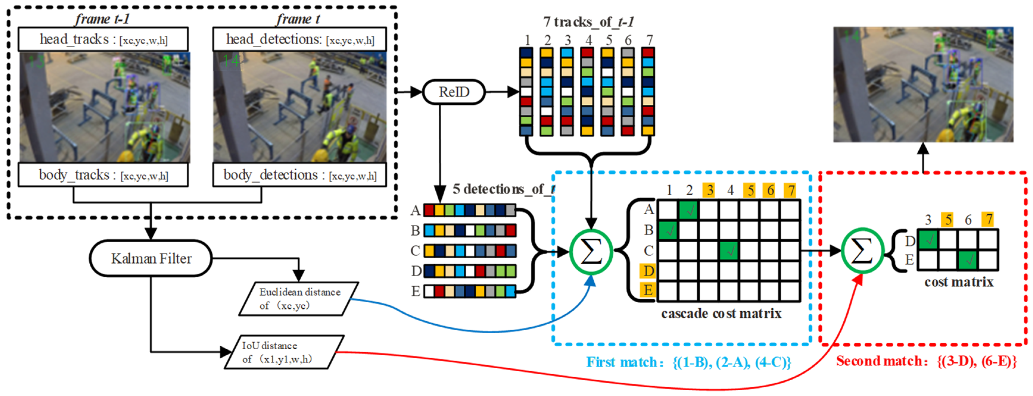
As shown in Figure 3, there are seven tracks of frame t − 1 and five detections of frame t; after the first match, (1-B), (2-A) and (4-C) were matched; the remaining (3-D) and (6-E) were successfully obtained in the second match. The tracking ID and detection ID are represented by the rows and columns in the cosine distance cost matrix. To match the tracking ID with the current frame, the Hungarian algorithm (Algorithm 1) is used. If the value is below the cosine similarity threshold of 0.2 and meets the tracking ID criteria, it is considered a successful match.

We modify the trackers in four ways:

(1) The Mahalanobis distance is modified to the Euclidean distance (23) in KF, to avoid the influence of covariance matrix divergence. $x_t={\left[x_c,y_c,a,h,v_x,v_y,v_a,v_h\right]}^T$ is the predicted vector of frame t over the state distribution (8-d) from frame t − 1, and it $y_t={\left[x_c,y_c,a,h,0,0,0,0\right]}^T$ refers to the detector’s measurements in frame t.

$$\begin{array}{l}Mahalanobisdistance=\sqrt{{\left(x_t-y_t\right)}^T{P}^{-1}\left(x_t-y_t\right)}\\ Euclideandistance=\sqrt{{\left(x_t-y_t\right)}^T\left(x_t-y_t\right)}\end{array}$$

(23)

(2) The head trajectory can be used as a reference to improve body accuracy. Because the head has limited motion and a fixed size, its use helps reduce errors in direction detection, ensuring that the tracker and imputer are not misled by incorrect detection results.

(3) The cost matrix uses a variable threshold (2 × head width), which reduces the number of for-loops to two. The vanilla DeepSORT cost matrix utilizes a fixed threshold of 9.4877, but variable thresholds maintain the visual principle of “near-big, far-small”. Therefore, a smaller threshold is crucial when a worker is far from the camera, has a small head size, and shows minimal movement.

(4) Additional constraints to add a new body ID. The unmatched detections of vanilla DeepSORT were directly added as a new ID, which might have resulted in inflation. The confidence level must be approximately 0.8 or no less than 0.95 during the range intervals near the edge. This effectively filters out most false positives.

Algorithm 1: Two Stages of the Matching Algorithm for the Trackers

Input: M ← number of workers; A ← number of frames; Two detections set: $D=\left\{d_i^j\left|1\le i\le M;1\le j\le A\right.\right\};D_{remain}=\left\{d_{i,remain}^j\left|1\le i\le M_{remain};1\le j\le A\right.\right\};$ Output: Two tracks set: $T_{matched}=\left\{t_i^j\left|1\le i\le N_{matched};1\le j\le A\right.\right\};T_{un\_matched}=\left\{t_i^j\left|1\le i\le N_{un\_matched};1\le j\le A\right.\right\};$ 1: for frame j in A do: 2:   $D^j=\left\{d_1^j,d_2^j,d_3^j,\dots d_{M^j}^j\right\}$ /*observations from the detector and ReID at j*/    $x^j=\left\{x_1^j,x_2^j,x_3^j,\dots x_{N^j}^j\right\}$ /*posterior state from KF by j − 1 */ 3. /*The First match: assignment to list of matches, unmatched_tracks, unmatched_detections:*/    $C^j\leftarrow C_{cosine}\left(D^j,x^j\right)+C_{Euclidean}\left(D^j,x^j\right)$ /*cost matrix at j */    Use the linear $\mathrm{Hungarian}\mathrm{algorithm}\mathrm{to}\mathrm{solve}{C}^j$.    if ($c_{\cos ine}$ > 0.2 and $c_{Euclidean}$ > 2 × head_width):     $T_{matched}\leftarrow t_i^j$ $\mathrm{that}\mathrm{matched}\mathrm{with}{d}_i^j$     $T_{un\_matched}\leftarrow t_i^j$$\mathrm{that}\mathrm{is}\mathrm{not}\mathrm{matched}\mathrm{with}{d}_i^j$     $D_{remain}\leftarrow d_i^j$$\mathrm{that}\mathrm{is}\mathrm{not}\mathrm{matched}\mathrm{with}{t}_i^j$ 4. /*The second match: for the remaining detecting-ID in $D_{remain}$*/    $C^j\leftarrow C_{cosine}\left({D_{remain}}^j,{x_{un\_matched}}^j\right)+C_{1-IoU}\left({D_{remain}}^j,{x_{un\_matched}}^j\right)$    Use the linear $\mathrm{Hungarian}\mathrm{algorithm}\mathrm{to}\mathrm{solve}{C}^j$.    if ($c_{1-IoU}$ > 0.7) or (match_times = 0 and $0.1\le c_{\cos ine}\le 0.2$):     $T_{matched}\leftarrow t_i^j$ $\mathrm{that}\mathrm{matched}\mathrm{with}{d}_{i,remain}^j$     $T_{un\_matched}\leftarrow t_i^j$$\mathrm{that}\mathrm{is}\mathrm{not}\mathrm{matched}\mathrm{with}{d}_{i,remain}^j$     $D_{remain}\leftarrow d_{i,remain}^j$$\mathrm{that}\mathrm{is}\mathrm{not}\mathrm{matched}\mathrm{with}{t}_i^j$

In this study, we utilized a Market-1501-based [34] 512-d vector for appearance information, which was better than the original 128-d vector of ReID (see Appendix A) in DeepSORT because an extensive feature dimension is appropriate for small objects such as heads.

4.2. Intra-Frame Processing

Intra-frame processing is used to reduce false positives and keep true positive detections, which can be treated as the pre-processing stage of the tracker’s inputs, as shown in Figure 2. Intra-frame processing contains the delete process and store process.

First, we need to filter out false positives of detected heads. Compared to height, human heads have smaller differences in size, so heads closer to the camera usually have clearer visual features and greater confidence scores than those that are farther away. Therefore, following the perspective principle of “near-big, far-small” and the detection confidence score, it is possible to filter out most of the false positive detected heads, as shown in Figure 4.

The head closest to the camera has the highest priority, and any heads with a confidence score of no less than 99% will be considered as true positives directly. After sorting by center vertical coordinates, we determine whether to delete the corresponding item based on the difference in height values and confidence scores between adjacent head boxes, as shown in Algorithm 2.

Algorithm 2: Filter out False Positives of Detected Heads

Input:   M ← number of detected heads; N ← number of remain heads; j = frame;     $D_{head}=\left\{d_i^j\left|1\le i\le M;1\le j\le A\right.\right\};$$d_i^j={\left[x_c,y_c,w,h,confidence,class\_id=1\right]}_{i=1}^M$ Output: $D_{head}^{del}=\left\{d_i^j\left|1\le i\le N;1\le j\le A\right.\right\};$$D_{head}^{remain}=\left\{d_i^j\left|1\le i\le N;1\le j\le A\right.\right\};$ 1: $D_{head}\leftarrow sort\left\{d_i^j,y_c\right\};$        /*sorted by head center yc*/ 2: while i + 1 < M − 1 do:    ${\Delta }_i\leftarrow d_i^j-d_{i+1}^j;$    if ${\Delta }_i$ < −5:           /*two heads are very close, maybe FP in here*/     if $d_i^j\left[4\right]$ ≥ 99%:       /* confidence ≥ 0.99*/       $D_{head}^{del}\leftarrow d_i^j$       /*delete i*/     elif $d_{i+1}^j\left[4\right]\ge d_i^j\left[4\right]$:       $D_{head}^{del}\leftarrow d_{i+1}^j$      /*delete i + 1*/     else:       $D_{head}^{del}\leftarrow d_i^{j}and{d}_{i+1}^j$  /*delete i and i + 1*/    i += 1 3: $D_{head}^{remain}\leftarrow D_{head}-D_{head}^{del}$

Second, we need to filter out false positives of detected bodies. Body detections are prone to instability when encountering occlusions or blurring. IoU and keypoints will be taken as conditions to delete unstable bodies in Algorithm 3; first, calculate the IoU between each pair of bounding boxes and if the value is greater than the given threshold (iou_threshold = 0.6), the lower confidence box is deleted; second, check the number of keypoints to ensure at least two body joints are in the box.

Algorithm 3: Filter out False Positives of Detected Bodies

Input:   M ← number of detected bodies; N ← number of remain bodies; j = frame;     $D_{body}=\left\{d_i^j\left|1\le i\le M;1\le j\le A\right.\right\};$$d_i^j={\left[x_c,y_c,w,h,confidence,class\_id=0\right]}_{i=1}^M$ Output: $D_{body}^{del}=\left\{d_i^j\left|1\le i\le N;1\le j\le A\right.\right\};$$D_{body}^{remain}=\left\{d_i^j\left|1\le i\le N;1\le j\le A\right.\right\};$ 1: for i, k in M do:    $Io{U}_i\leftarrow Compute\_IoU\left(d_i^j,d_i^{j+1}\right);$    if $Io{U}_i$ ≥ 60%:          /*two bodies are very close, maybe FPs in here*/     $D_{body}^{del}\leftarrow \min \left(d_i^j\left[4\right],d_i^{j+1}\left[4\right]\right)$  /*lower confidence deleted*/     i += 1     k += 1 2: for i in length(keypoints) do:   /*if the body has no more than two effective keypoints in total*/   if torch.sum (one_key[:, −1] ≥ 0.05) < 2:     $D_{body}^{del}\leftarrow d_i^j$          /*lower confidence deleted*/     i += 1 3: $D_{body}^{remain}\leftarrow D_{body}-D_{body}^{del}$

After these filtering steps, the remaining heads and bodies are passed to the store process. To handle potential crowd scenarios where multiple heads may occupy a single body location, we employed Python dictionaries (head_sequence_set and body_sequence_set) to store data. This approach allows for persistent tracking even when individuals enter or exit the field of view. Additionally, this method mitigates indexing issues that may arise due to variable head–body pairings, such as the example provided:

body_head_matched_ids = [(3, 0), (0, 1), (2, 2), (None, 3), (4, None), (1, 4)]

By deferring matching to the inter-frame tracking stage, our method can utilize appearance features in addition to intra-frame location data, thus avoiding the potential identity confusion caused by false positives, as shown in Figure 4.

In summary, the intra-frame processing stage employs a combination of confidence scores, size principles and keypoint analysis to refine head and body detections, reducing false positives and preparing the data for more accurate inter-frame tracking using the RseNet-50-based [10] head-integrated keypoint R-CNN model.

4.3. Inter-Frame Matching

Since head detection can aid in body detection [10], head tracking can likewise assist in body tracking, as described in this section. Because a less occluded head has an inclusion relationship with the entire body, the corresponding tracking can be achieved through bidirectional matching algorithms.

Inter-frame matching refers to associating the heads and bodies in consecutive frames. Unlike the traditional matching procedure of “head to head” or “body to body” in vanilla DeepSORT, we have expanded the scope of association to “head to body”.

Because the head and body do not belong to the same recognition category ($class\_id=0$ for body; $class\_id=1$ f or head), it is meaningless to directly use the appearance features of the head to match a body but this is very useful for filtering newly added tracking IDs, as shown in Algorithm 4. This process can provide additional checking conditions for new IDs. In the case of mixed tracking, the correspondence between the body and head does not need to be calculated in every frame but only during the track ID initialization frame.

The head feature is the critical factor in identifying a worker in practical construction scenarios, which may lead to dilemmas in the annotation of tracking IDs in manual labeling. Due to the size of the head being relatively small and fixed, we used the Euclidean distance of the bounding box center (3 × width) and a higher confidence threshold (95%) to restrict the newly added head’s tracking ID in Algorithm 3. Based on the assumption that the head tracking is more accurate than the body tracking, the newly added body should not be around those already-existing heads by the IoU threshold of 0.8.

Whenever there is a newly added ID, we calculate the elements z of the cost matrix as (24) and use Algorithm 4 to find the corresponding head or body ID.

$$z=\frac{1-\mathit{modified}\text{\_}\mathit{IoU}}{\mathit{confidence}}$$

(24)

$$\mathit{modified}\text{\_}\mathit{IoU}=\frac{\mathit{body}\cap \mathit{head}}{\mathit{min}\left(\mathit{body},\mathit{head}\right)}$$

(25)

where the modified_IoU in (25) is no longer focused on the union area of the body and head, but on the smaller area. This type of calculation tends to retain a high-overlap “head to body” pair, and the low-confidence pair will lose priority to an extent.

Algorithm 4: Matching of “Head to Body” across Frames

Input: MT ← number of tracked heads; NT ← number of tracked bodies; j = frame; $T_{body}=\left\{t_{i,body}^j\left|1\le i\le N_T;1\le j\le A\right.\right\};$$t_{i,body}^j={\left[x_c,y_c,w,h,confidence,class\_id=0\right]}_{i=1}^{N_T}$ $T_{head}=\left\{t_{i,head}^j\left|1\le i\le M_T;1\le j\le A\right.\right\};$$t_{i,head}^j={\left[x_c,y_c,w,h,confidence,class\_id=1\right]}_{i=1}^{M_T}$ $L_{body,head}=\left\{\left(t_{i,body}^j,t_{a,head}^j\right)\left|1\le i\le N_T;1\le j\le A;1\le a\le N_T\right.\right\};$ Output: $L_{body,head}$ 1: if $\exists I{D}_{head}\notin T_{head}$:    for k in $L_{body,head}$ do:     /*find the closest head, and calculate the Euclidean distance of the center*/     if Euclidean $\left|I{D}_{head}-t_{a,head}^j\right|$ > 3×w and $I{D}_{head}\left[4\right]$ > 0.95:       $T_{head}\leftarrow I{D}_{head}$ 2: if $\exists I{D}_{body}\notin T_{body}$:    for k in $L_{body,head}$ do:     /*find the closest body, and calculate the IoU*/     if IoU $\left(I{D}_{body},t_{a,head}^j\right)$ > 0.8 and $I{D}_{a,head}^j\ne None$:       $T_{body}\leftarrow I{D}_{body}$ 3: if $T_{head}\leftarrow I{D}_{head}$$\mathrm{or}{T}_{body}\leftarrow I{D}_{body}$: /*matching of new added head–body pairs*/     $\forall C^j\in \cos \mathrm{t}\text{\_}\mathrm{matrix},C^j\leftarrow \frac{1-\mathrm{modified}\text{\_}\mathrm{IoU}}{\mathrm{confidence}}$$\mathrm{when}{C}^j\le 1.0$;               $C^j\leftarrow 100000$$\mathrm{when}{C}^j>1.0$;     Use the linear $\mathrm{Hungarian}\mathrm{algorithm}\mathrm{to}\mathrm{solve}{C}^j$     # row_indices, col_indices = linear_assignment(cost_matrix)     $L_{body,head}\leftarrow \left(I{D}_{body},I{D}_{head}\right)$

By adding head tracking, the weakness of relying solely on body tracking can be overcome. Figure 5 (the frame #37 in video-3) shows the effective processing of inter-frame matching from left to right images: the left image is the detector’s outputs, while the middle image is the tracker’s outputs and the right image is the final results. Head and body IDs can obtain the pair-wise relationship and stable trajectories successfully. The newly added head ID = 17 in the middle image (confidence = 92.2% in the left image) was deleted as a false positive association and did not affect the final tracking outputs.

In vanilla DeepSORT, the matching algorithm was only restricted to two frames (t − 1 and t) as the Markov property in the KF in (2), whereas former frames (1, 2 … t − 2) were forgotten. Then, unmatched head or body detections could be directly and easily treated as a new track ID for the next frame; consequently, if the ReID feature vector of the current frame is not good enough due to occlusions or blurring, better feature vectors from previous frames will be replaced and cannot be recovered. Using the head as a benchmark can maintain correspondence with past frames during the bad modification of body features in the current frame; the “head to body” matching reduces possible ID errors effectively.

Note: to clearly understand how head tracking aids in body tracking, please refer to Appendix B for the calculation details.

4.4. Evaluation Metrics

CLEAR MOT [35] proposed the IDF1, MOTA and MOTP metrics in (26)–(28).

$$IDF1=\frac{2\times IDTP}{2\times IDTP+IDFP+IDFN}$$

(26)

$$MOTA=1-\frac{{\displaystyle {\sum }_i\left(IDF{P}_i+IDF{N}_i+IDS{W}_i\right)}}{{\displaystyle {\sum }_{i}G{T}_i}}\in \left(-\infty ,\left.1\right]\right.$$

(27)

$$\mathit{MOTP}=\frac{{\displaystyle {\sum }_{i,t}{d}_{i,t}}}{{\displaystyle {\sum }_i{c}_i}}\in \left(0,1\right)$$

(28)

where True Positive ID (IDTP) is the number of correctly assigned IDs throughout the entire video; False Positive ID (IDFP) is the number of incorrect IDs; False Negative ID (IDFN) is the number of missed IDs; IDSW is the identity switches of one object; GT means the number of manually labeled ground truth boxes; $i$ is one frame in video set; $t$ is a worker identity; $d$ refers to the distance between the prediction box and ground truth box, $d$ may be assigned as the IoU distance.

IDTP does not have the same value as TP. The former emphasizes maintaining ID consistency, whereas TP primarily focuses on bounding box IoU. IDTP can only be obtained after the tracking association calculation is complete, whereas TP can be obtained during the earlier detection stage. The same is true for IDFP and FP, and IDFN and FN.

IDF1 gauges the proportion of correctly identified detections to the mean count of ground truth and computed detections. It offers a fair assessment of all trackers based on their identification precision and recall through their harmonic mean [36].

MOTA measures the combined errors of IDFNs, IDFPs and IDSW. However, IDFPs have a greater influence than IDFNs and IDSW. For instance, if the GT tracking target has an ID error, it results in an increment of IDFP + 1. On the other hand, if the GT does not have a corresponding detection, it is considered missing, resulting in IDFN + 1. Changes in IDFPs will lead to an increase in IDFNs but not vice versa. It is important to note that MOTA does not include a measure of localization error.

To compensate for this, MOTP measures a tracker’s ability to accurately estimate object positions, regardless of its proficiency in recognizing object configurations and maintaining consistent trajectories. It primarily evaluates positional accuracy, which is more relevant to the detector’s performance than the overall performance of the tracker. As a result, MOTChallenge removes MOTP as an evaluation metric.

HOTA [6] balances the effect of three accuracies: detection, association and localization. Equations (29) and (30) decompose HOTA into separate DetA and AssA scores.

$${\mathit{HOTA}}_{\alpha }=\sqrt{\frac{{\displaystyle \sum _{c\in \left\{\mathit{TP}\right\}}\mathcal{A}}(c)}{\left|\mathit{TP}\right|+\left|\mathit{FN}\right|+\left|\mathit{FP}\right|}}=\sqrt{\mathit{Det}{A}_{\alpha }\cdot {\mathit{AssA}}_{\alpha }}$$

(29)

$$\mathit{HOTA}={\displaystyle {\int }_0^1{\mathit{HOTA}}_{\alpha }d\alpha \approx \frac{1}{19}{\displaystyle \sum _{\alpha \in \left\{0.05,0.1,\cdots 0.95\right\}}{\mathit{HOTA}}_{\alpha }}}$$

(30)

where $\alpha$ is the localization threshold of IoU, with 19 different distinct values (0.05 to 0.95 in 0.05 intervals) for integral calculation; c is one worker ID. More details of the HOTA formula can be found in [6].

HOTA identified two errors in ID distinction for tracking: ID switches (IDSWs) and ID transfers (IDTRs). IDSW is designed for continuous trajectories, while IDTR is designed for intermittent trajectories.

IDSW calculates the frequency at which a tracked trajectory switches its matched GT identity. It is worth mentioning that this definition is applicable only while the target is within the field of view. IDSW occurs when, in consecutive frames, the same worker has varying IDs, but it is restricted to TP and not FN. If a trajectory abruptly vanishes, it will not be counted as IDSW.

IDTR happens when one worker exits the frame and another worker enters the subsequent frame, but with the former’s ID. IDTR is common in scenarios involving frequent entry and exit. When worker A leaves frame-i, worker B enters frame-i + 1. If worker B is mistakenly recognized as worker A in frame-i + 1, worker A’s ID will be transferred to worker B, but IDSW will not be added since worker A was interrupted. Therefore, IDTR is also considered an undesirable behavior during tracking, which MOTA could not consider.

Fortunately, HOTA can effectively resolve IDTR errors [6]. The IDSW in the CLEAR MOT evaluation only measures short-term tracking and cannot accurately assess long-term tracking. HOTA can evaluate the global long-term tracking by comparing FN and FP in the matched trajectories.

5. Results and Discussion

The proposed tracking method achieved an IDF1 of 97.609%, MOTA of 95.191% and HOTA of 78.884% on the testing dataset of nine videos [2] with a total of 41 workers. Additionally, the method achieved an IDSW of 0, even in scenarios with heavy occlusions. This is the first report of the IDSW value since previous research on tracking workers.

The model is implemented using Python 3.8.8 and PyTorch 1.8.0. The method is based on the GitHub code [37], containing KF and Hungarian algorithms. The computer has one NVIDIA RTX 3080 GPU, an Intel(R) Core(TM) i9-10900K CPU @ 3.70 GHz and one 32 GB RAM with Win10. The testing dataset of nine videos is the same as [2,38], with a resolution of 1920 × 1080 and 30 FPS; more details can be found in [2].

The ground truth data with frame-ID, track-ID and bounding box in a four-tuple (x, y, width, height) were manually annotated as follows: <frame>, <id>, <bb_x>, <bb_y>, <bb_width>, <bb_height>, <conf = 1>, <x = −1>, <y = −1>, <z = −1>. This was performed with TrackEval [39].

5.1. Quantitative Results

Table 2. Performance of our tracking method on the testing dataset.

Metrics		Video-1	Video-2	Video-3	Video-4	Video-5	Video-6	Video-7	Video-8	Video-9	Combined
1	MOTA↑ (%)	100	94.08	93.943	93.582	94.833	98.859	95.44	96.843	93.972	95.191
2	IDF1↑ (%)	100	97.04	96.966	96.824	97.468	99.431	97.73	98.422	97.007	97.609
3	HOTA↑ (%)	93.023	77.601	81.446	75.7	74.801	76.911	78.273	81.799	77.446	78.884
4	AssA↑ (%)	93.023	79.784	86.066	78.962	81.28	85.451	80.484	83.341	78.149	83.296
5	AssRe↑ (%)	94.298	84.026	89.916	84.525	87.219	89.145	85.352	86.762	84.28	87.83
6	AssPr↑ (%)	94.298	84.026	90.052	83.247	84.142	88.895	84.634	86.689	83.016	86.976
7	LocA↑ (%)	92.568	83.922	86.915	82.642	82.643	81.798	84.326	85.815	85.614	84.725
8	IDSW↓	0	0	0	0	0	0	0	0	0	0
9	Frag↓	0	4	7	21	22	4	6	10	12	86
10	Hz↑	9.05	6.01	5.69	5.96	7.11	6.69	6.62	5.33	6.82	6.58
11	MT	1	3	9	5	5	4	4	6	4	41

(‘↑’ means higher is better, ‘↓’ means lower is better).

presents a comprehensive analysis of the performance evaluation outcomes for the nine videos across seven metrics: MOTA, IDF1, HOTA, AssA, AssRe, AssPr and LocA. It is important to note that the aggregated value in the final row does not result from a simple average of individual video scores due to variations in total frames; instead, the cumulative frames of all videos are considered.

The method consistently demonstrates stability and reliability across diverse scenarios and conditions, as shown in Figure 6. The challenge for tracking algorithms, particularly in video 3, with the highest number of workers, is exemplified by HOTA reaching 81.446%, which is marginally higher than the combined score of 78.884%, thereby highlighting the effectiveness of the crowd-tracking method.

5.2. Comparision of Other SOTA Methods

Pedestrian tracking on roads presents a relatively straightforward task from a programming standpoint, despite some inherent complexities and uncertainties in traffic environments. In contrast, construction sites pose a greater challenge due to their dynamic nature. The simplicity of pedestrians’ movement patterns further contributes to the relative ease of tracking on roads.

Table 3. Performance of classical pedestrian tracking method on the testing dataset.

Metrics		DeepSORT	ByteTrack	Deep OC_SORT	BoTSORT	OC_SORT	Strong_SORT	TransTrack	UniTrack
1	MOTA↑ (%)	69.914	62.515	56.429	60.699	66.002	56.698	39.345	27.441
2	IDF1↑ (%)	79.771	81.829	74.471	77.365	80.633	77.065	70.459	61.887
3	HOTA↑ (%)	68.418	66.915	62.425	63.208	66.596	63.893	57.607	49.201
4	AssA↑ (%)	74.585	77.995	71.394	73.429	76.166	74.7	72.685	63.686
5	AssRe↑ (%)	78.896	82.717	75.462	76.777	80.316	78.679	76.712	68.208
6	AssPr↑ (%)	84.488	83.637	83.043	85.385	86.221	84.348	82.495	74.389
7	LocA↑ (%)	85.353	80.694	82.01	82.833	82.657	82.058	80.222	69.791
8	IDSW↓	21	5	51	8	10	12	7	15
9	Frag↓	101	107	178	180	168	140	161	268
10	Hz↑	1.77	9.09	8.33	7.14	8.47	7.69	5.13	4.30

(‘↑’ means higher is better, ‘↓’ means lower is better).

highlights eight state-of-the-art pedestrian tracking methods employed in recent years, particularly in the context of worker tracking. However, these methods exhibit considerable disparities in application domains, tracked objects and technical challenges. Consequently, selecting the most suitable tracking techniques for practical applications is crucial, as it ensures alignment with the diverse needs and requirements of different scenarios.

The codes of ByteTrack [7], Deep OC_SORT [26], BoTSORT [29], OC_SORT [9] and Strong_SORT [30] are from [40]. These five methods were retrained on 26.6 K images of CrowdHuman, MOT17, Cityperson and ETHZ datasets [7]. TransTrack [24] and UniTrack [31] are in the authors’ original codes, and DeepSORT uses an implementation from [41]. These three methodologies rely on vanilla YOLOX-x (yolox_x.pth, 756 MB).

As displayed in Table 3, YOLOX-based DeepSORT achieved the highest HOTA and MOTA scores, at 68.418% and 69.914%, respectively, but exhibited the lowest FPS (1.77) and the worst IDSW score (21). In contrast, ByteTrack demonstrated the best performance, with an IDF1 score of 81.829%, the fastest FPS (9.09) and the lowest IDSW score (5). Despite these achievements, none of these pedestrian tracking methods surpasses our proposed bidirectional tracking method.

5.3. Discussion

Compared with the unidirectional method, the bidirectional method has the following advantages:

(1)

Low dependency of detection DNN

The bidirectional approach allows the tracker to modify the results of the detector in reverse with imputers and refiners. Therefore, poor detections (ResNet-50 [10]) in the current frame will be modified into acceptable outputs and saved into head or body sequence sets for the next frame’s prediction. Thus, these poor detections will not greatly change the value of the covariance matrix.

(2)

Application of head tracking aid in body tracking

Head cues’ distinctive attributes, including low variation, visibility and reduced occlusion, contribute to their effectiveness in tracking tasks. In tracking algorithms, the utilization of head appearance features for body tracking marks a novel approach. Worker tracking, far from being a mere metric comparison, demonstrates its practicality in complex situations like the occlusions depicted in Figure 7 and Figure 8. Despite individual differences in head shape, the relatively consistent size of heads compared to other body parts ensures more reliable appearance features compared to limbs.

In Figure 7, from frames #4 to #14, workers with ID = 2 and ID = 4 of the same categories are moving in the opposite direction. In frame #16, ID = 2 loses the detection of the head and body until frames #19 and #22, respectively. After calculating, ID = 2 maintained continuous tracklets during the overlap by ID = 4, proving its effectiveness in handling intra-class occlusions.

In Figure 8, due to the obstruction of the fence category, only a few appearance features are visible in the worker category ID = 0. Frame #79 demonstrates that the scaled-down bounding box of ID = 0 was repaired to a normal height and width, indicating that inter-class occlusions can be fixed even during bad detections.

(3)

Avoidance of the impact of KF divergence issues

The prediction of the whole body’s speed can now be replaced by the speed of the head, instead of solely relying on KF prediction. The head’s speed can serve as a reference to refine body velocity predictions in the KF. If body bounding box coordinates are inaccurate, the correct head coordinates can be employed to correct them, preventing the tracker and imputer from being misled by faulty detections.

For instance, in the top row of Figure 9, the body detector’s output for the left worker’s full-body box in frames 112 to 114 shows an unexpected increase in the x-coordinate (ID 4). The expected trend is a decrease as the worker moves leftward, but the detection error pushes the x-coordinates to the right (upper row: 667.91 → 668.17 → 666.25). Conversely, the head’s x-coordinate accurately reflects the leftward movement (lower row: 668.50 → 653.50 → 648.00). By utilizing head-based linear interpolation, the x-coordinate of the full-body bounding box can be corrected to the correct value (lower row: 666.65 → 665.5 → 660.5), ensuring accurate tracking.

(4)

Focus on metrics performance with ID errors

Addressing identity errors can be efficiently achieved with meticulous handling of new head or body IDs, as outlined in the intra-frame processing and inter-frame matching sections. By not immediately assigning unmatched detections to new identities, these methods can significantly reduce false positives (FPs) and false negatives (FNs), as demonstrated by Algorithms 2–4. These heuristic algorithms streamline the process by avoiding the need for retraining and effectively leveraging head information for identity association. By attentively managing new IDs, they contribute to enhanced tracking system performance, presenting a simple, effective and cost-efficient solution. This approach is particularly suitable for practical applications due to its wide applicability.

The main limitation of the proposed method is the fact that many innovations are heuristic and difficult to fully prove using mathematical formulas. Another limitation is that it is not possible to completely abandon the use of KF to estimate velocity values.

A potential future research direction is to track worker movement data, obtain movement characteristics and make trajectory predictions.

6. Conclusions

This article introduced a training-free tracking method for tracking workers. The novel method has a bidirectional interaction mechanism between the detector and tracker, which allows head information to supply more stable and precise navigation for body tracking. We have also analyzed in detail the mathematical reasons for the non-convergence phenomenon, and the proposed method can successfully prevent the problem of non-convergence KF in traditional one-way tracking and significantly reduce identity errors regarding workers through the designed newly added ID-checking algorithms. During testing, our method achieved an HOTA of 78.884%, an MOTA of 95.191% and an IDSW of 0 across nine video datasets, demonstrating that the method remains highly effective even in scenarios with serious occlusions or non-convergence issues.

References

- Teizer, J. Status quo and open challenges in vision-based sensing and tracking of temporary resources on infrastructure construction sites. Adv. Eng. Inform. 2015, 29, 225–238. [Google Scholar] [CrossRef]
- Xiao, B.; Xiao, H.; Wang, J.; Chen, Y. Vision-based method for tracking workers by integrating deep learning instance segmentation in off-site construction. Autom. Constr. 2022, 136, 104148. [Google Scholar] [CrossRef]
- Golizadeh, H.; Hon, C.K.H.; Drogemuller, R.; Hosseini, M.R. Digital engineering potential in addressing causes of construction accidents. Autom. Constr. 2018, 95, 284–295. [Google Scholar] [CrossRef]
- Freimuth, H.; Koenig, M. Planning and executing construction inspections with unmanned aerial vehicles. Autom. Constr. 2018, 96, 540–553. [Google Scholar] [CrossRef]
- Guo, H.; Yu, Y.; Skitmore, M. Visualization technology-based construction safety management: A review. Autom. Constr. 2017, 73, 135–144. [Google Scholar] [CrossRef]
- Luiten, J.; Os, A.A.; Dendorfer, P.; Torr, P.; Geiger, A.; Leal-Taixé, L.; Leibe, B. HOTA: A Higher Order Metric for Evaluating Multi-object Tracking. Int. J. Comput. Vis. 2021, 129, 548–578. [Google Scholar] [CrossRef] [PubMed]
- Zhang, Y.; Sun, P.; Jiang, Y.; Yu, D.; Weng, F.; Yuan, Z.; Luo, P.; Liu, W.; Wang, X. ByteTrack: Multi-Object Tracking by Associating Every Detection Box. arXiv 2022, arXiv:2110.06864. [Google Scholar] [CrossRef]
- Wojke, N.; Bewley, A.; Paulus, D. Simple Online and Realtime Tracking with a Deep Association Metric. In Proceedings of the 24th IEEE International Conference on Image Processing (ICIP), Beijing, China, 17–20 September 2017; pp. 3645–3649. [Google Scholar] [CrossRef]
- Cao, J.; Pang, J.; Weng, X.; Khirodkar, R.; Kitani, K. Observation-Centric SORT: Rethinking SORT for Robust Multi-Object Tracking. arXiv 2022, arXiv:2203.14360. [Google Scholar] [CrossRef]
- Liu, Y.; Zhou, Z.; Wang, Y.; Sun, C. Head-Integrated Detecting Method for Workers under Complex Construction Scenarios. Buildings 2024, 14, 859. [Google Scholar] [CrossRef]
- Dendorfer, P.; Ošep, A.; Milan, A.; Schindler, K.; Cremers, D.; Reid, I.; Roth, S.; Leal-Taixé, L. MOTChallenge: A Benchmark for Single-Camera Multiple Target Tracking. arXiv 2020, arXiv:2010.07548. [Google Scholar] [CrossRef]
- Leal-Taixé, L.; Milan, A.; Reid, I.; Roth, S.; Schindler, K. MOTChallenge 2015: Towards a Benchmark for Multi-Target Tracking. arXiv 2015, arXiv:1504.01942. [Google Scholar] [CrossRef]
- Ciaparrone, G.; Sánchez, F.L.; Tabik, S.; Troiano, L.; Tagliaferri, R.; Herrera, F. Deep Learning in Video Multi-Object Tracking: A Survey. arXiv 2019, arXiv:1907.12740. [Google Scholar] [CrossRef]
- Ren, S.; He, K.; Girshick, R.; Sun, J. Faster R-CNN: Towards Real-Time Object Detection with Region Proposal Networks. arXiv 2016, arXiv:1506.01497. [Google Scholar] [CrossRef] [PubMed]
- Redmon, J.; Divvala, S.; Girshick, R.; Farhadi, A. You Only Look Once: Unified, Real-Time Object Detection. arXiv 2015, arXiv:1506.02640. [Google Scholar] [CrossRef]
- Duan, K.; Bai, S.; Xie, L.; Qi, H.; Huang, Q.; Tian, Q. CenterNet: Keypoint Triplets for Object Detection. arXiv 2019, arXiv:1904.08189. [Google Scholar] [CrossRef]
- Vaswani, A.; Shazeer, N.; Parmar, N.; Uszkoreit, J.; Jones, L.; Gomez, A.N.; Kaiser, Ł.; Polosukhin, I. Attention Is All You Need. arXiv 2017, arXiv:1706.03762. [Google Scholar] [CrossRef]
- Girshick, R. Fast R-CNN. arXiv 2015, arXiv:1504.08083. [Google Scholar] [CrossRef]
- Bewley, A.; Ge, Z.Y.; Ott, L.; Ramov, F.; Upcroft, B. Simple Onlne and Realtime Tracking. In Proceedings of the 23rd IEEE International Conference on Image Processing (ICIP), Phoenix, AZ, USA, 25–28 September 2016; pp. 3464–3468. [Google Scholar] [CrossRef]
- He, K.; Gkioxari, G.; Dollár, P.; Girshick, R. Mask R-CNN. arXiv 2018, arXiv:1703.06870. [Google Scholar] [CrossRef]
- Bashar, M.; Islam, S.; Hussain, K.K.; Hasan, M.B.; Rahman, A.B.M.A.; Kabir, M.H. Multiple Object Tracking in Recent Times: A Literature Review. arXiv 2022, arXiv:2209.04796. [Google Scholar] [CrossRef]
- Shuai, B.; Berneshawi, A.; Li, X.; Modolo, D.; Tighe, J. SiamMOT: Siamese Multi-Object Tracking. arXiv 2021, arXiv:2105.11595. [Google Scholar] [CrossRef]
- Meinhardt, T.; Kirillov, A.; Leal-Taixe, L.; Feichtenhofer, C. TrackFormer: Multi-Object Tracking with Transformers. arXiv 2021, arXiv:2101.02702. [Google Scholar] [CrossRef]
- Sun, P.; Cao, J.; Jiang, Y.; Zhang, R.; Xie, E.; Yuan, Z.; Wang, C.; Luo, P. TransTrack: Multiple Object Tracking with Transformer. arXiv 2020, arXiv:2012.15460. [Google Scholar] [CrossRef]
- Google. Google Colaboratory. 2023. Available online: https://colab.research.google.com/ (accessed on 29 August 2023).
- Maggiolino, G.; Ahmad, A.; Cao, J.; Kitani, K. Deep OC-SORT: Multi-Pedestrian Tracking by Adaptive Re-Identification. arXiv 2023, arXiv:2302.11813. [Google Scholar] [CrossRef]
- Yang, M.; Han, G.; Yan, B.; Zhang, W.; Qi, J.; Lu, H.; Wang, D. Hybrid-SORT: Weak Cues Matter for Online Multi-Object Tracking. arXiv 2023, arXiv:2308.00783. [Google Scholar] [CrossRef]
- Duan, P.; Zhou, J.; Goh, Y.M. Spatial-temporal analysis of safety risks in trajectories of construction workers based on complex network theory. Adv. Eng. Inform. 2023, 5, 101990. [Google Scholar] [CrossRef]
- Aharon, N.; Orfaig, R.; Bobrovsky, B.-Z. BoT-SORT: Robust Associations Multi-Pedestrian Tracking. arXiv 2022, arXiv:2206.14651. [Google Scholar] [CrossRef]
- Du, Y.; Zhao, Z.; Song, Y.; Zhao, Y.; Su, F.; Gong, T.; Meng, H. StrongSORT: Make DeepSORT Great Again. arXiv 2022, arXiv:2202.13514. [Google Scholar] [CrossRef]
- Wang, Z.; Zhao, H.; Li, Y.L.; Wang, S.; Torr, P.; Bertinetto, L. Do Different Tracking Tasks Require Different Appearance Models? arXiv 2021, arXiv:2107.02156. [Google Scholar] [CrossRef]
- Zhang, Y.; Wang, C.; Wang, X.; Zeng, W.; Liu, W. FairMOT: On the Fairness of Detection and Re-Identification in Multiple Object Tracking. arXiv 2020, arXiv:2004.01888. [Google Scholar] [CrossRef]
- Chu, P.; Wang, J.; You, Q.; Ling, H.; Liu, Z. TransMOT: Spatial-Temporal Graph Transformer for Multiple Object Tracking. arXiv 2021, arXiv:2104.00194. [Google Scholar] [CrossRef]
- Zheng, L.; Shen, L.; Tian, L.; Wang, S.; Bu, J.; Tian, Q. Person Re-identification Meets Image Search. arXiv 2015, arXiv:1502.02171. [Google Scholar] [CrossRef]
- Bernardin, K.; Stiefelhagen, R. Evaluating Multiple Object Tracking Performance: The CLEAR MOT Metrics. Eurasip J. Image Video Process. 2008, 2008, 246309. [Google Scholar] [CrossRef]
- Ristani, E.; Solera, F.; Zou, R.S.; Cucchiara, R.; Tomasi, C. Performance Measures and a Data Set for Multi-Target, Multi-Camera Tracking. arXiv 2016, arXiv:1609.01775. [Google Scholar] [CrossRef]
- KubaRurak. Detectron2-Deepsort-Repo. 2021. Available online: https://github.com/KubaRurak/detectron2-deepsort-repo (accessed on 31 August 2023).
- Konstantinou, E.; Lasenby, J.; Brilakis, I. Adaptive computer vision-based 2D tracking of workers in complex environments. Autom. Constr. 2019, 103, 168–184. [Google Scholar] [CrossRef]
- JonathonLuiten. TrackEval. 2021. Available online: https://github.com/JonathonLuiten/TrackEval (accessed on 31 August 2023).
- Mikel-Brostrom. YOLO_Tracking. 2023. Available online: https://github.com/mikel-brostrom/yolo_tracking#real-time-multi-object-segmentation-and-pose-tracking-using-yolov8--yolo-nas--yolox-with-deepocsort-and-lightmbn (accessed on 31 August 2023).
- pmj110119. YOLOX_Deepsort_Tracker. 2021. Available online: https://github.com/pmj110119/YOLOX_deepsort_tracker (accessed on 31 August 2023).
- Xiao, B.; Kang, S.-C. Vision-Based Method Integrating Deep Learning Detection for Tracking Multiple Construction Machines. J. Comput. Civ. Eng. 2021, 35, 04020071. [Google Scholar] [CrossRef]
- Xiao, B.; Lin, Q.; Chen, Y. A vision-based method for automatic tracking of construction machines at nighttime based on deep learning illumination enhancement. Autom. Constr. 2021, 127, 13. [Google Scholar] [CrossRef]
- Drive, G. Deepsort_Parameters. 2023. Available online: https://drive.google.com/drive/folders/1xhG0kRH1EX5B9_Iz8gQJb7UNnn_riXi6 (accessed on 31 August 2023).
Figure 1.
Types of identity errors in tracking workers.
Figure 2.
Overview of the proposed tracking method.
Figure 3.
Framework of the head_tracker or body_tracker.
Figure 4.
Examples of deleted false positives during intra-frame processing.
Figure 5.
Process images of the inter-frame matching.
Figure 6.
Testing videos’ tracking outputs at their final frames.
Figure 7.
Example of intra-class occlusions in video 3.
Figure 8.
Example of inter-class occlusions in video 7.
Figure 9.
Example of body’s reverse movement for ID = 4.