
Escaping Stagnation through Improved Orca Predator Algorithm with Deep Reinforcement Learning for Feature Selection


1
Escuela de Ingeniería Informática, Universidad de Valparaíso, Valparaíso 2362905, Chile
2
Escuela de Ingeniería Informática, Pontificia Universidad Católica de Valparaíso, Valparaíso 2362807, Chile
*
Author to whom correspondence should be addressed.
Mathematics 2024, 12(8), 1249; https://doi.org/10.3390/math12081249
Submission received: 28 March 2024
/
Revised: 17 April 2024
/
Accepted: 18 April 2024
/
Published: 20 April 2024
(This article belongs to the Special Issue Evolutionary Computation and Applications)
Abstract
:Stagnation at local optima represents a significant challenge in bio-inspired optimization algorithms, often leading to suboptimal solutions. This paper addresses this issue by proposing a hybrid model that combines the Orca predator algorithm with deep Q-learning. The Orca predator algorithm is an optimization technique that mimics the hunting behavior of orcas. It solves complex optimization problems by exploring and exploiting search spaces efficiently. Deep Q-learning is a reinforcement learning technique that combines Q-learning with deep neural networks. This integration aims to turn the stagnation problem into an opportunity for more focused and effective exploitation, enhancing the optimization technique’s performance and accuracy. The proposed hybrid model leverages the biomimetic strengths of the Orca predator algorithm to identify promising regions nearby in the search space, complemented by the fine-tuning capabilities of deep Q-learning to navigate these areas precisely. The practical application of this approach is evaluated using the high-dimensional Heartbeat Categorization Dataset, focusing on the feature selection problem. This dataset, comprising complex electrocardiogram signals, provided a robust platform for testing the feature selection capabilities of our hybrid model. Our experimental results are encouraging, showcasing the hybrid strategy’s capability to identify relevant features without significantly compromising the performance metrics of machine learning models. This analysis was performed by comparing the improved method of the Orca predator algorithm against its native version and a set of state-of-the-art algorithms.
MSC:
68T05; 68T20; 68W50; 90C59; 90C271. Introduction
Over the years, optimization mechanisms have significantly evolved, in tandem with the rise in scientific knowledge, as evidenced by the considerable progress in this field of study [1]. In this context, artificial intelligence has led the most significant innovations, and within this realm, bio-inspired optimization algorithms, especially those employing biomimetic approaches, have achieved significant benefits [2]. Despite their proven efficiency in solving a variety of complex optimization problems [3], these methods face a crucial challenge: stagnation at local optima. Many works have faced this issue as a problem to be normally solved by using sophisticated exploration techniques to visit other places of the search spaces [4,5,6]. However, this stagnation can be viewed as an opportunity to exploit promising zones of the search space with more focused and controlled diversification, potentially enhancing the algorithm’s performance and accuracy.
In swarm intelligence algorithms, the stagnation problem typically occurs when solutions converge to a local optimum rather than the desired global optimum [7]. This is primarily due to artificial agents being guided by local information in their vicinity, leading to premature convergence to suboptimal solutions. When the swarm becomes trapped in a local optimum, exploring other regions of the search space becomes challenging. This convergence is altered with random exploration processes. This implies that targeted tactics do not always enrich the search for the global optimum but are sometimes guided by a more random process. Although this approach may open new areas for exploration [8,9], it does not necessarily ensure a more effective path to optimal solutions.
In this research, we pioneer the synergy of the Orca predator algorithm (OPA) and deep Q-learning (DQL), aiming to harness the strengths of both to identify and exploit promising solutions more effectively, building on the foundational work detailed in [10]. Traditional methodologies often fall short by prematurely converging on local optima; our strategy, however, capitalizes on such convergences, treating them as gateways for directed exploration towards areas of promise. The selection of OPA was meticulous, driven by its intricate parameter requirements and the profound influence of its calibration. This methodology is designed to be adaptable and suitable for application to other techniques with similar functional characteristics. The fusion of OPA and DQL marks a notable innovation in tackling optimization challenges, merging OPA’s biomimetic prowess in swiftly pinpointing areas worth exploring with DQL’s precision in refining searches within these zones.
Despite our proposal’s significant advancements, we also face challenges inherent in integrating optimization techniques with deep learning algorithms [11]. One of the main challenges in this field is the management of high-dimensional search spaces, which often lead to a higher probability of generating similar solutions. Additionally, the computational complexity of combining OPA with DQL raises practical concerns regarding computational resources and execution time, particularly in large-scale problems [12]. We acknowledge the potential of our approach in various optimization scenarios while also considering that its applicability and effectiveness may need to be tailored to the specific characteristics and complexities of each unique problem set.
The proposal will be evaluated on the feature selection (FS) problem, aiming to identify a subset of features that offers comparable results with less computational effort. This is particularly relevant in datasets with irrelevant, noisy, and high-dimensional data [13,14]. The dataset selected for evaluation is the Heartbeat Categorization Dataset [15], available on Kaggle. This dataset contains electrocardiogram signals of heartbeats, which can be normal or affected by various arrhythmias and myocardial infarctions. The dataset includes 188 features, reflecting the dimensionality of our problem. To validate our proposal, the improved Orca predator algorithm will be rigorously compared with its native version and various established techniques already considered state-of-the-art, underscoring its competitive edge and potential for setting new benchmarks in the field.
This research is committed to exploring the frontiers of bio-inspired optimization methods and machine learning, seeking not only to advance in theory and methodology but also in the practical application of these techniques to real-world problems. With a focus on feature selection in complex datasets, this study aims to overcome limitations and pave new paths for future research in this exciting and rapidly evolving field.
The structure of this work is presented as follows: Section 2 provides a robust analysis of the current work on hybridizations between learning techniques and metaheuristics. Section 3 details the conceptual framework of the study, emphasizing the biomimetic principles of OPA, the formal description of DQL, and the formulation of FS. Section 4 explains how reinforcement learning is integrated into the Orca predator algorithm. Section 5 outlines the phases of the experimental design. Section 6 discusses the results achieved, underscoring the approach’s effectiveness in feature selection. Finally, the conclusions and future work are presented in Section 7.
2. Related Work
In the realm of computational intelligence, mainly biomimetic algorithms, there has been a concerted and vigorous effort to enhance the search capabilities of these algorithms. This endeavor has involved not only the augmentation of existing models with more sophisticated decision-making and optimization strategies but also the integration of innovative computational techniques that mimic natural processes more closely [16]. These improvements have been manifested in numerous ways, from increased speed and accuracy in finding optimal solutions to a more profound ability to tackle high-dimensional and dynamically changing environments. Initial strides have been made towards devising new strategies for swarm intelligence algorithms, augmenting their search capabilities through formulations specifically designed to modulate the balance between exploration and exploitation. These efforts underscore the potential of bio-inspired methods to autonomously modulate their behavior. Some recent examples can be seen in [17,18,19,20,21,22,23,24,25,26].
Swarm-based intelligence methods have firmly established themselves as a robust framework for navigating and optimizing search spaces. However, the integration of machine learning into these algorithms represents a pivotal advancement, significantly amplifying their efficacy [27]. By harnessing machine learning, these algorithms gain unprecedented capabilities to learn from, adapt to, and effectively address the intricacies of complex problem spaces.
This synthesis of swarm intelligence and machine learning facilitates the creation of algorithms that not only traverse search spaces with enhanced efficiency but also demonstrate a superior ability to identify and utilize optimal solutions across varied problem domains. This interdisciplinary fusion is driving noteworthy progress in computational intelligence, equipping swarm-based optimization strategies with a level of adaptability and learning proficiency previously unattainable [28,29].
Such evolutionary strides are crucial for the development of sophisticated methods tailored to meet the challenges posed by complex optimization landscapes. At the heart of this transformative shift is the goal to harmonize the inherent exploratory capabilities of swarm intelligence algorithms with the predictive and analytical prowess of machine learning. Achieving this equilibrium ensures a dynamic interplay between exploration and exploitation, enabling the algorithms to navigate and solve complex problems more effectively [30].
Exploring closer the fusion of metaheuristics with reinforcement learning unveils a robust corpus of research dedicated to augmenting the efficiency of optimization algorithms through this multidisciplinary approach [31]. This integration has led to significant advancements across several research domains. Innovations in local search optimization [32], dynamic parameter tuning [33], and the identification of promising search areas represent key areas of progress [34]. Studies have demonstrated the efficacy of this integration in enhancing algorithmic intelligence and adaptability, contributing to fields ranging from optimization challenges in theoretical contexts to practical applications like neural network training and cloud computing load balancing [35,36]. This collective body of work highlights a pivotal shift towards more sophisticated, efficient, and adaptive optimization strategies capable of addressing complex problems across a wide range of disciplines [37].
Integrating bio-inspired techniques and machine learning also plays a fundamental role in feature selection. This approach is an essential component in the effectiveness of machine learning models. Recent research has explored various methodologies and techniques to enhance feature selection. For instance, ref. [38] offers a comprehensive review of the use of metaheuristic algorithms in feature selection, suggesting paths for future research in developing or modifying these algorithms for classification tasks. In [39], the performance of recent metaheuristic algorithms in feature selection is evaluated, highlighting the challenges and opportunities in this field.
The models presented in [40,41] demonstrate the application of hybrid approaches that combine optimization techniques and deep reinforcement learning for feature selection in network intrusion detection. Additionally, ref. [42] compiles a series of research on feature selection, where a taxonomy of objective functions is presented, and related metrics are classified into four categories: classifiers, metaheuristics, features, and statistical tests. This classification facilitates effective comparison of different feature selection methodologies, focusing on metaheuristics’ implementation and hybridization strategies.
Finally, ref. [43] introduces a technique for predicting customer churn in the telecommunications sector. The Archimedes optimization algorithm is employed for optimal feature selection, combined with a hybrid deep learning model for customer churn prediction. The study is notable for its focus on efficient feature selection and hyperparameter tuning, achieving significant improvements in the accuracy and effectiveness of the predictive model. The study’s results indicate the high efficiency of the proposed technique compared to other methods, achieving outstanding accuracy.
3. Preliminaries
In this section, we introduce the conceptual framework of our study, focusing on the biomimetic principles underlying the Orca predator algorithm, providing a formal description of deep reinforcement learning through deep Q-learning, and outlining the formulation of feature selection. This framework forms the foundation of our approach, integrating these distinct yet complementary components to address the challenges at hand.
3.1. Biomimetic Orca Predator Algorithm
The Orca predator algorithm is inspired by the predatory tactics of orcas, leveraging their strategic hunting behaviors as a foundation for its operational framework [44]. Recognized for their complex social structures and cooperative hunting strategies, orcas utilize echolocation to navigate and communicate within their aquatic territories, orchestrating coordinated assaults on their prey. In this algorithmic model, a potential solution is conceptualized as an n-dimensional vector, with the collective solution space denoted by .
OPA operates through two primary stages: the chase and attack phases, each embodying distinct aspects of orca hunting patterns. The chase phase comprises two distinct actions: herding the prey towards the water’s surface and surrounding it to prevent escape. This is regulated by a parameter p, which dictates the likelihood of executing either action, based on a comparison with a random value r within the interval . Should , the algorithm opts for the herding strategy; otherwise, it proceeds with encirclement. The subsequent attack phase mirrors the orcas’ approach to narrowing the gap with their prey, employing precision and cooperation to secure their target. The efficacy of OPA hinges on its ability to mimic these intricate behaviors, requiring accurate sensory data and collaborative decision-making processes to optimize the search for solutions.
3.1.1. Chase Phase
This strategy operates under two distinct environmental scenarios. The initial scenario emerges when a diminutive shoal of fish constricts the spatial domain available for the orca’s navigation. Conversely, the second scenario unfolds as an expansive shoal of fish broadens the orca’s operational hunting territory. In response to these varying conditions, the algorithm delineates two specific approaches for engaging with the prey.
The dynamics of velocity and spatial positioning are computed by Equations (1)–(4). In this strategy, delineates the velocity according to the initial chase tactic, while marks the corresponding spatial coordinate of the i-th orca at moment t. Analogously, and are defined for the alternative chase strategy. The variable is the general coordinate of the i-th orca at time t, and is the optimal position among the orcas, signifying proximity to the prey or the most efficient strategy at time t. The term M quantifies the mean position within the orca assembly, with a, b, and d representing random variables uniformly distributed in , and e spans a range of . The parameter F encapsulates the influence or attractive force exerted by one agent upon another, and q, lying within , dictates the likelihood of selecting a specific method for prey pursuit.
With the prey now accessible at the water’s surface, the subsequent maneuver involves encircling the target. Orcas, utilizing sonar for communication, ascertain their ensuing positions through coordination with proximate members of their pod. It is posited that orcas adjust their locations based on the coordinates of three orcas chosen at random. The calculation of their positions post-maneuver is articulated through Equations (5)–(7), providing a mathematical representation of this coordinated movement.
where denotes the maximal iteration count, whereas , , and represent three distinct orcas chosen at random from the collective, ensuring ≠≠. The variable corresponds to the spatial coordinate of the i-th orca subsequent to adopting the tertiary strategy for pursuit at the iteration t.
Throughout the chase, orcas leverage acoustic signals to ascertain the prey’s whereabouts, modulating their spatial orientation in response. This instinctive behavior prompts orcas to either persist in the pursuit, contingent on the perceived proximity of the prey, or to halt and maintain their current position if the prey seems to be distancing itself.
3.1.2. Attack Phase
After encircling their prey, orcas execute a coordinated attack by taking turns entering the formed circuit to feed. Upon feeding, they revert to their original positions within the enclosure to allow another orca to partake in the feeding process. Assuming that four orcas correspond to the optimal attack positions within the circle, other orcas may choose to join the circuit based on their positional preferences. The direction in which orcas return to the enclosure circle after feeding, in preparation for replacement, is determined by the positions of randomly selected neighboring orcas. This behavioral pattern is precisely characterized through Equations (8)–(10).
In this context, symbolizes the velocity vector of the i-th orca engaged in prey pursuit at iteration t, while denotes the velocity vector of the i-th orca returning to the rendezvous circuit during the same iteration t. The positions of the four orcas optimally positioned within the circuit are represented by , , , and . Additionally, , , and are three orcas randomly selected from the population during the pursuit, with the constraint ≠≠. The positional update of the i-th orca after the attack phase at iteration t is expressed as . Furthermore, is a random value chosen from the interval , and is a random number within the range .
Subsequent to this phase, orcas employ sonar to detect the prey’s location and adjust their positions accordingly, mirroring the pursuit process. The lower boundary limit (lb) of the problem’s potential range dictates the orcas’ positional adjustments, conforming to the stipulations outlined in the algorithm proposed by [44].
Algorithm 1 details the orca predator procedure. The pseudocode requires the definition of inputs such as population size (S), probabilities for selecting methods (p and q), and dimensionality (n), aiming to produce the best solution. Thus, the algorithm begins by initializing the objective function and randomly computing the first generation of S orcas (Line 1). For each orca and each decision variable, positions and velocities are assigned randomly (Lines 4–6). The fitness of each orca is calculated using the objective function defined in the optimization problem, and the best orca is identified. If an orca is better than the best solution achieved, then this solution is updated.
| Algorithm 1: Pseudocode for the orca predator method. |
 |
Subsequently, the algorithm enters a loop to produce generations of orcas until a predefined iteration limit is reached (Line 16). Within this loop, each orca is processed. The algorithm selects three random orcas (Line 18). Based on the probability p, the algorithm decides whether to perform the chase phase to drive the prey or encircle the prey for each variable (Lines 19–29). If p is more significant than a random value, the chase phase is executed by either driving the prey or encircling it based on the value of q (Lines 20–28). If p is less than a random value, the attack phase is performed for each variable (Lines 29–33). The fitness of each orca is computed again (Line 34), and the best solution achieved is updated if an orca is found to be better (Lines 36–40). The algorithm concludes by returning the post-processed results and visualization (Line 42).
3.2. Deep Reinforcement Learning
Reinforcement learning (RL) is an advanced machine learning technique focusing on autonomous agents striving to maximize rewards through their actions [45]. These agents learn by trial and error, identifying actions that lead to greater rewards, both immediate and long-term, a distinguishing feature of RL [46].
In the RL process, agents continually interact with their environment, involving key components such as the value function, policy, and occasionally, a model of the environment [47,48,49,50]. The value function evaluates the effectiveness of the agent’s actions in the environment, and the agent’s policy adjusts based on received rewards.
Q-learning, a fundamental technique in RL, focuses on establishing a function to assess the effectiveness of a specific action in a given state at time t [51,52]. The Q function updates using Equation (11):
where is the learning rate and is the discount factor. is the reward obtained after performing action .
Deep Reinforcement Learning (DRL) integrates deep learning techniques with RL, enabling addressing problems with greater complexity and dimensionality [53]. In DRL, deep neural networks approximate value functions or policies. Deep Q-Learning is a DRL technique that uses a neural network to approximate the Q value function to measure the expected cumulative reward for acting in a particular state. The Q value function learns through an iterative process when the agent takes actions in the environment and receives rewards.
In DQL, the Q function is defined as , where represents the current state, the action taken by the agent at time t, and the network weights [54]. The Q function is updated by using Equation (12):
where, and represent the new state and action at time , respectively. The parameter , known as the learning rate, regulates the magnitude of the update to the Q value function at each training step. A high value of accelerates the adaptation of the Q function to environmental changes, being beneficial in the initial stages of learning or in highly dynamic environments. However, an excessively high learning rate can cause a disproportionate response to random variations in rewards, leading to instability in learning [54]. On the other hand, a lower promotes a more gradual and stable learning process but may prolong the time required to achieve convergence. The factor , known as the discount factor, assigns relevance to future rewards compared to immediate ones. A value close to 1 encourages the agent to give almost equal importance to long-term rewards as to current ones, thereby incentivizing strategies that aim to maximize long-term benefits. In contrast, a lower prioritizes short-term rewards, which is advantageous in scenarios where future rewards are less predictable or when effective policies are required in reduced time horizons. Finally, is the reward received after executing action in state . represents the parameters of a target neural network that is periodically updated with the values of to improve training stability.
A distinctive feature of DQL is its use of replay memory, which constitutes a crucial part of its learning architecture [55,56]. Replay memory stores the agent’s past experiences in the form of tuples . Each tuple represents an individual experience of the agent, where is the current state, the action taken, the reward received, and the subsequent state. This approach of storing and reusing past experiences aids in enhancing the efficiency and effectiveness of the learning process, allowing the agent to learn from a more diverse set of experiences. With that, it reduces the correlation between consecutive learning sequences, a critical aspect to avoid over-dependence on recent data and to promote more generalized learning. Additionally, the mini-batch technique is implemented for sampling experiences from replay memory during the training process [57]. Instead of learning from a single experience at each step, the algorithm randomly selects a mini-batch of experiences. This batch sampling method contributes to the stability of learning by promoting the independence of samples and allows for more efficient use of computational resources.
Finally, learning in DQL is guided by a loss function according to Equation (13), which measures the discrepancy between the estimated Q and target values.
where y is the target value, calculated by Equation (14):
Here, is the reward received after taking action in state , and is the discount factor, which balances the importance of short-term and long-term rewards. The formulation represents the maximum estimated value for the next state , according to the target network with parameters . is the Q value estimated by the evaluation network for the current state and action , using the current parameters . In each training step in DQL, the evaluation network receives a loss function backpropagated based on a batch of experiences randomly selected from the experience replay memory. The evaluation network’s parameter, , is then updated by minimizing the loss function through the stochastic gradient descent (SGD) function. After several steps, the target network’s parameter, , is updated by assigning the latest parameter to . After a period of training, the two neural networks are trained stably.
Lastly, the epsilon-greedy [58] strategy in DQL crucially balances exploration and exploitation. It does this by initially favoring exploration with a probability of for selecting actions randomly and gradually shifting towards exploitation, choosing actions that maximize the Q function with a probability of . As the agent gains more knowledge, decreases, effectively transitioning from exploration to exploitation. This approach prevents the agent from settling into suboptimal strategies, ensuring adaptability and learning from diverse experiences.
3.3. Feature Selection
Feature selection is an integral component in data preprocessing that identifies and selects a subset of relevant features (variables, predictors) for use in model construction [59]. It is crucial in enhancing the efficiency of machine learning models by eliminating redundant and irrelevant data, thus streamlining the computational process and potentially improving model performance [60,61].
Formally, let us consider a dataset with a set of features and a class label Y. The objective of feature selection is to find a subset such that and the predictive power of concerning Y is maximized. This process involves evaluating the importance of each feature in D and retaining only those that contribute significantly to our understanding of Y.
There are three primary approaches to feature selection [62,63]: filter methods, wrapper methods, and embedded methods. Filter methods rank features based on statistical measures independent of any learning algorithm. Wrapper methods use a predictive model to score feature subsets and are computationally intensive, as they involve training models on different subsets. Embedded methods perform feature selection as part of the model training process and are specific to particular algorithms.
We focus on the wrapper approach, particularly its application in selecting features that provide high classification accuracy while minimizing computational resources. In this approach, subsets of features are iteratively evaluated using a specific learning algorithm, and the subset that yields the highest classification performance is selected. This process can be computationally expensive due to the need to train a model for each subset.
Our work utilizes an improved bio-inspired metaheuristic algorithm to optimize the feature selection process. Each potential solution in this algorithm represents a subset of features encoded as a binary string where one indicates the inclusion of a feature and zero is its exclusion. The algorithm iteratively refines these solutions, guided by the learning model’s performance on these subsets [64]. The performance of these subsets is evaluated using metrics like score and accuracy. score provides a balance between precision and recall, while accuracy measures the proportion of correctly predicted instances [65].
Feature selection is undoubtedly a vital step in the data preprocessing phase, aiding in reducing the dimensionality of the dataset, curtailing overfitting, and enhancing the generalizability and efficiency of the learning models [61]. Therefore, our work contributes to this field by applying an advanced metaheuristic approach to optimize the feature selection process, thereby striking a balance between model complexity and computational efficiency.
4. Developed Solution
Our proposed solution integrates the Orca predator algorithm with deep Q-learning for dynamically optimizing OPA’s parameters. This approach leverages the predatory behavior of orcas and DQL’s management of large state and action spaces to enhance feature selection efficiency. OPA, inspired by orca hunting strategies [44], offers an innovative optimization approach, while DQL addresses high-dimensional space challenges in complex combinatorial problems [66].
DQL plays an essential role in transitioning towards exploitation, particularly in the later stages of the optimization process. As OPA explores the solution space by mimicking orcas’ collaborative and adaptive strategies in their natural habitat, DQL refines this exploration by targeting the most promising regions. This shift from exploration to exploitation is efficiently managed through DQL’s epsilon-greedy policy, significantly enhancing the selection of optimal actions as the model accumulates knowledge.
OPA operates as a metaheuristic where each orca represents an independent search agent, exploring the solution space characterized by a binary vector. These vectors represent selected features from the database, with each vector being individually evaluated through a variety of machine learning algorithms, such as decision trees (DT), random forests (RF), support vector machines (SVM), and extremely randomized trees (ERT). score and accuracy derived from these evaluation methods provide crucial feedback to OPA about the quality of the solutions, thereby allowing the orcas to adjust their strategies and explore bounded promising areas of the solution space.
DQL intervenes in this dynamic adaptive process by providing a sophisticated reinforcement learning-based strategy to regulate the operational parameters of OPA. DQL accumulates experiences from the evaluations of the orcas, including rewards based on the diversity of solutions and performance metrics. These experiences are essential for updating the decision policies in OPA, precisely calibrating the probabilities and parameters that guide both the exploration and exploitation of the search space. Through the implementation of replay memory, DQL learns from past experiences, enabling it to anticipate and maximize future rewards. This leads to a significant and iterative improvement in feature selection, constantly refining the solution search process.
Figure 1 illustrates in detail the flow of the proposed solution process, highlighting the synergy between OPA and DQL in this advanced optimization method. It underscores how the interaction between these two components leads to a more efficient and effective search for optimal solutions, combining OPA’s nature-inspired exploration with DQL’s outcome-oriented and adaptive learning strategy.
The core of our methodology is embodied in the pseudocode of Algorithm 2. The algorithm begins by taking data from a dataset, such as dimensionality and row data, trying to find the best solution. Then, it continues by initializing a swarm of orcas and setting up the initial state and action parameters based on performance metrics.
| Algorithm 2: Pseudocode for the improved orca predator method. |
 |
The main loop of the hybridization continues until a specified iteration limit equal to the original version is reached. During each iteration, every orca in the swarm is processed. First, it selects three random orcas and updates the position and velocity of each orca. These two steps are also equivalent to the original version. Next, a machine learning technique is invoked to compute fitness (Line 8). This process uses the solution stored in the orca, corresponding to an n-dimensional vector composed of zeros and ones. The machine learning method generates a trained model only with selected columns (ones of the vector).
We strongly emphasize critical performance metrics in evaluating our machine learning model, notably the score and accuracy. We have adopted a comprehensive multi-objective strategy to enhance the model’s effectiveness. This approach does not just focus on maximizing these essential metrics but also includes the solution diversity metric and a reduction component aimed at optimizing the balance between the number of features used and the total available features. This optimization is crucial for streamlining our algorithm and making it more efficient in feature selection.
Integrating individual performance metrics into a unified measure known as the feature efficiency index (FEI) is central to our study. The FEI is designed to capture the holistic performance of the model by synthesizing the score, accuracy, diversity of solutions, and effectiveness of the feature reduction strategy. This composite measure is calculated through a carefully designed linear scalarization method, as detailed in Equation (15), allowing us to gauge the overall efficiency and effectiveness of the model in utilizing the selected features.
In the above formula, represents the weights assigned to each pair of objective functions, ensuring that the total influence of each function is balanced and the sum of all weights equals 1. This normalization is critical, as it maintains the proportionality and relevance of each function relative to the others, ensuring no single metric disproportionately influences the FEI. The values represent upper bounds to minimize within single-objective functions, ensuring that the FEI strives for optimal values across all dimensions.
The terms and refer to the current and best values of the objective functions, respectively, allowing the FEI to dynamically adjust as improvements are found during the optimization process. The objective functions and aim to maximize the score and accuracy, respectively, while seeks to minimize the diversity (heterogeneity) of solutions, and focuses on maximizing the use of non-dominant features (reduction strategy). With that, a reward is generated based on performance metrics. Changes in the score, accuracy, diversity, and reduction are computed by comparing the current values with previous values.
where , , , and serve as weights, each assigned to quantify the significance of corresponding terms in the reward calculation. The terms and represent the scores of the current and previous best orcas, respectively. Similarly, and refer to the accuracies of the current and previous best orcas, respectively. Both scores and accuracies, values close to 1 indicate a good performances.
Diversity is evaluated using the Euclidean distance between the positions of each pair of orcas across the entire swarm. For a set of orcas, with each individual’s position denoted by the vector , diversity is determined in accordance with Equation (17).
where S denotes the total number of orcas, n represents the dimension of the solution space, and and are k-th decision variables of solutions and , respectively. Values close to 0 note a good performance. Finally, the reduction metric is calculated by determining the percentage of columns not accessed by the most proficient orca in relation to the total number of available columns. Again, values close to 1 indicate a good performances.
We can see that the reward function is tailored to encourage solutions that not only enhance performance in terms of score and accuracy but also maintain diversity and utilize a reduced number of features. Next, updating of states and actions is conducted through the DQL process (Line 12). In this process, the state is a vector composed by the current performance metrics and the diversity of the orca swarm, and is represented as follows:
In the training phase of the DQL process, the formulation of states is a critical aspect, as it provides the necessary context for decision-making [67]. This state design (Equation (18)) ensures that all critical dimensions of the problem are represented, allowing DQL to make informed adjustments in OPA’s operational parameters. This information is compiled in real time and feeds into DQL to facilitate continuous and adaptive adjustment decisions.
The actions in the DQL process are decisions on how to adjust OPA’s operational parameters, identified as a, b, d, and e. These parameters are vital in defining the movement and adaptation strategies of the orcas in OPA. Specifically, a and b control the intensity and direction of the orcas’ movement, respectively, influencing their capacity to explore the solution space. On the other hand, d and e determine the orcas’ sensitivity to environmental signals, affecting their ability to adapt and converge towards optimal solutions.
In the DQL process, two key neural networks are implemented: (1) the evaluation network, which is constantly updated with new experiences, and (2) the target network, which provides a stable estimation of Q-function values and is periodically updated to stabilize the learning process [68]. This approach helps mitigate issues associated with data correlation and rapid changes in Q-estimation, which can lead to unstable learning. The loss function in DQL is critical for calibrating the evaluation network. Huber loss, a combination of mean squared and absolute errors, is employed, as it is less sensitive to outliers in predictions and provides more stable training. The loss is calculated by comparing the predictions of the evaluation network with the target values generated by the target network. Here, the gradient descent algorithm plays a crucial role, as it adjusts the network parameters by minimizing this loss function, allowing the model to learn from its errors effectively.
During DQL training, each accumulated experience, based on the performance and diversity of the orcas’ solutions, contributes to updating the parameters to be improved. The aim is to achieve an effective balance between exploring new areas and exploiting the most promising ones in the solution space. The parameter tuning is carried out through an iterative reinforcement learning process, where the DQL model evaluates the impact of different configurations of these parameters on the overall system performance. Through the reward function, DQL identifies which adjustments in these parameters enhance the efficacy of the search, thus guiding the evolution of the exploration and exploitation strategy in OPA.
The parameters of OPA are optimized using the DQL training function, which employs a neural network for continuous estimation of the Q-function values, along with a memory buffer to store experiential data (referenced in Lines 18–19). The neural network facilitates the DQL model’s learning process, enabling it to maximize expected long-term rewards by refining its predictions based on feedback from environmental interactions. Concurrently, the memory buffer plays a crucial role by preserving a record of accumulated experiences during these interactions. Each recorded experience encapsulates the system’s current state, the action executed, the reward obtained, and the subsequent state achieved post-action. This historical data empowers the model to extract lessons from previous scenarios, thereby boosting its predictive accuracy and adaptability in new situations—a critical aspect for enhancing decision-making efficiency over time.
Action selection follows an epsilon-greedy strategy, ensuring a proper mix between exploration and exploitation. After executing an action, the new state and reward are observed (Lines 21–22) and stored in the memory buffer. Once sufficient experiences are accumulated, a mini-batch is extracted to train the evaluation network. This training process involves updating the target network with state–action pairs and their corresponding target values, simultaneously adjusting the values of parameters (Lines 26–27).
This iterative DQL training method is reintegrated into the main algorithm, allowing optimization cycles to continue. With each iteration, DQL adapts and improves its policy, thus refining OPA’s search for focused exploitation in a promising area of the solution space. This leads to more precise and efficient feature selection for machine learning models (Line 16). This iterative procedure is repeated, progressively refining the solutions proposed by the orcas through a reward that reflects both the quality of the solution in terms of model performance and the exploitation of new potential solutions. With each iteration, DQL adapts, improving its policy and refining OPA’s search for more effective exploitation of the solution space, leading to a more precise and efficient feature selection for machine learning models.
Finally, regarding computational complexity, our metaheuristic exhibits complexity, where n denotes the dimension of the problem and k represents either the number of iterations or the population size, encapsulating the total number of function evaluations throughout the algorithm’s execution. We also evaluate the complexity of the DQL algorithm, which is generally [69,70], with M indicating the sample size and N the number of network parameters, both essential for thorough dataset analysis. Despite the potentially large values of M and N, they remain fixed, making the integration of DQL a justifiable increase in computational demand for superior outcomes. Additionally, the continual advancement in computing technology significantly mitigates the impact of this heightened complexity.
5. Experimental Setup
We used a rigorous quantitative methodology to evaluate our proposal, comparing the hybrid approach with the traditional version of the optimization algorithm. Moreover, we tested each machine-learning method independently. This involved detailed planning, execution, and assessment, including statistical testing and in-depth analysis.
5.1. Methodology
To evaluate the enhanced metaheuristic’s performance rigorously, we have established a comprehensive quantitative methodology that aligns with the principles outlined in [71]. Our approach involves a comparative analysis between the solutions provided by our proposed hybridization, the native version of the optimization algorithm, and the results generated by machine learning working alone. For that, we employed the following methodological strategy:
- Preparation and planning: Define specific multi-objective goals for feature selection effectiveness, aiming to minimize the number of selected features while simultaneously maximizing accuracy and the score. Design experiments to systematically evaluate the enhanced technique under controlled conditions, ensuring a balanced optimization of these criteria.
- Execution and assessment: Perform a multi-faceted evaluation of the technique, assessing not only the quality of the solutions generated but also the computational efficiency and convergence properties. Employ rigorous statistical tests to compare the performance with baseline methods. Here, to evaluate data independence and statistical significance, we use the Kolmogorov–Smirnov–Lilliefors test for assessing sample autonomy and the Mann–Whitney–Wilcoxon test for comparative analysis. This approach involves calculating the fitness from each one executions per instance.
- Analysis and validation: Conduct thorough in-depth analysis to understand the deep Q-learning’s parameter influence and the orca predator algorithm’s behavior on the feature selection task. This involves iterating over a range of hyperparameters to fine-tune the model, using the dataset to validate the consistency and stability of the selected features. To ensure the validity of the results generated by our proposal, we conducted tests to evaluate the final outcomes. We can assure that all simulated experiments were carried out with reliability.
5.2. Dataset
Our research utilized the “ECG Heartbeat Categorization Dataset” from Kaggle [15], which comprises records of ECG signals indicative of various heart conditions. These signals are classified into five categories: Normal (N), Supraventricular (S), Ventricular (V), Fusion (F), and Unclassified (Q). The dataset is rich, with 188 distinct features per record, encapsulating the complexity of our problem space, represented as n. The dataset is divided into two primary files: the training set, containing 87,554 records, and the test set, with 21,892 records. For our analysis, we further split the test set equally into two parts: one half (10,946 records) is utilized for cross-validation to fine-tune the model parameters, while the remaining half is reserved for the final testing phase to evaluate the model’s performance. This significantly reduces the risk of overfitting.
We employed a strategic sampling approach to address class imbalance during training. For classes 1 (S), 2 (V), and 4 (Q), which had a larger number of records, we randomly selected a subset of 1000 records each. This was conducted to ensure that these classes did not overwhelm the learning process. In contrast, for class 3 (F), which had fewer instances, we included all 641 available records. This selective sampling was crucial to maintain a balanced representation across all classes, enhancing the classifier’s ability to identify each category accurately without bias.
During the testing or prediction phase, we utilized the available records. This comprehensive approach in the testing phase allowed us to assess the model’s performance across a diverse and complete range of data. In both the training and testing stages, we applied all 188 features in the dataset to the machine learning techniques, ensuring a thorough analysis and utilization of the available data. This exhaustive feature application was key to comprehensively training and evaluating the machine learning models, providing us with a detailed understanding of the dataset and the effectiveness of our approach.
5.3. Implementation Aspects
We conducted empirical assessments of the Orca predatory algorithm. These trials involved independent executions of four distinct machine learning models: decision tree (DT), random forest (RF), support vector machine (SVM), and extremely randomized trees (ERT). In subsequent stages, we evaluated the hybridization of the OPA algorithm with each of these classification techniques.
In [44], the parameter values yielding the best average performance regarding swarm behavior are described. Based on this, we developed a set of preliminary evaluations with a reduced test scenario in order to find the best initial configuration [72]. Setting q to notably boosts OPA performance, because the algorithm has more opportunities to search for solutions in a wide search space against the exploration phase than looking for a local search procedure. These tests generated good results, and we can observe that the a and d parameters take values closer to 1 than 0. The b value is kept random without unpredictable behavior. Finally, these experiments show the F value is always close to 2. Consequently, our proposal will be challenged to operate and improve in an initially adverse situation. We extracted results from 30 runs per algorithm, each run iterating 100 times and orcas. In order to identify how different values for the parameters affect the final performance, we plotted its values against the performance metrics, enabling us to analyze trends and optimal values that enhance the model’s effectiveness. This analysis will reveal which parameters are critical for the algorithm’s performance.
We established the following parameters for the deep Q-learning configuration: The state size was set to 5, with an action size of 40 to encompass a broad range of potential parameter adjustments in OPA. We constructed a sequential neural network with dense layers and dropout for regularization. The network consists of layers with 24 neurons each, using ReLU activation, and a final layer of size equal to the number of possible actions (40), with linear activation. The Huber loss function and the RMSprop optimizer with a learning rate of were used. Regarding the epsilon-greedy policy, we started with an epsilon value of 1.0, decaying to a minimum of to balance exploration and exploitation. Using a double Q-learning approach, the network trains with random experiences from a mini-batch during training and updating. The target network is updated every 50 training steps to stabilize the estimation of Q-values. The initial values for parameters and e, used in moving the orcas and updating their positions and velocities, are randomly generated in the range of [0, 1] at the start of each OPA algorithm execution. Table 1 summarizes the initial parameter values.
Another key aspect is the adaptation of OPA to the binary domain, which necessitates the inclusion of a binarization phase following alterations to the solution vector. In this instance, the transformation function utilized was the conventional sigmoid function. This entails that if , with representing a random value uniformly distributed within the interval , then, discretization is achieved by setting . Conversely, should this condition not hold, is applied.
Finally, we used Python 3.10 to code all algorithms. The computer used for each test had the following specifications: macOS 14.2.1 Darwin Kernel version 23 with an Ultra M2 chip and 64 GB of RAM. All codes are available in [73].
6. Results and Discussion
The initial comparative analysis between our approach and the traditional version of OPA focuses on the runtime. On one hand, we consider the time it takes to generate the solution vector, encompassing all necessary actions and the time required to process and evaluate fitness accuracy. On the other hand, the time spent on the classification phase using learning techniques is not considered because this phase is considered part of the model’s training process, where the primary focus is on achieving high accuracy and reliability rather than speed.
OPA achieves the best runtime in all the tests performed, with a value of 200 ms. In contrast, the best time achieved by OPADQL is 500 ms, which is even worse than the average time of OPA, equivalent to 220 ms. There are no instances where OPADQL’s runtime is inferior to OPA’s runtimes. However, it is important to note that although OPADQL does not outperform OPA in runtime, the difference is negligible. The anticipated benefit in terms of prediction accuracy and feature reduction justifies the additional execution time required by OPADQL.
Furthermore, we acknowledge the importance of examining how the selected features vary across different runs. To this end, we conducted several runs of the OPA and OPADQL methods, analyzing the consistency in feature selection. We found that, although there is inherent variability due to the stochastic nature of the algorithms, certain features tend to be selected more frequently, indicating their potential relevance to the problem at hand. We can see that discarded features are usually related to constant or poorly varied values since they do not provide useful information for differentiating between heartbeat categories, as well as those that offer redundant information.
Continuing with experimental results, Table 2 and Table 3 present our computational findings. Tables are structured into five sections, each comprising six rows corresponding to evaluation metrics. We define the best value as the optimal performance attained across each model and feature selection technique combination, highlighted using bold font. Conversely, the worst value signifies the least effective yield. The mean value provides an average of the results, while the standard deviation (std) value quantifies the variability in findings. Additionally, the median value and interquartile range (iqr) value represent the middle value and the spread of the middle 50% of performances. Regarding columnar representation, the notation n/o specifically denotes the absence of an optimizer method, indicating that algorithms were run without optimization techniques to enhance performance. In this context, all machine learning methods are employed to classify the dataset using all features. The best-performing methods are then identified, and their results are stored for comparative analysis.
OPA stands for a bio-inspired optimizer lacking a learning component, and OPADQL represents our enhanced version of OPA. Finally, we employ score, accuracy, diversity, reduction, and FEI for metrics. All of them were defined in the previous section. In the context of the score and accuracy, the OPADQL model exhibits a remarkable and consistent enhancement in performance when contrasted with the native OPA and non-optimized learning methods.
This improvement is particularly pronounced in models employing RF and SVM, underscoring the advanced capability of OPADQL in managing intricate feature selection challenges. This integration enables a more nuanced and precise feature selection process. Consequently, this leads to a significant boost in model performance, as evidenced by the higher F1 scores and accuracy rates, which are critical indicators of a model’s predictive power and reliability in classification tasks.
Concerning the diversity metric, an essential measure of the variation and uniqueness in the solutions generated, both OPA and OPADQL showcase commendable performances. However, OPADQL distinguishes itself by achieving marginally inferior values. This slight but critical advantage highlights the efficacy of the hybrid model in sustaining the comprehensive exploitation of the solution space.
The OPADQL’s ability to try to maintain a diverse set of solutions while simultaneously homing in on the most effective ones exemplifies its balanced approach to optimization. This diverse exploitation ensures that the algorithm does not prematurely converge to suboptimal solutions, thereby enhancing the robustness and reliability of the outcomes.
The results of the reduction metric are particularly striking. In this aspect, OPADQL outshines OPA by a significant margin, indicating a more proficient approach in maximizing the number of features while not preserving or even enhancing model accuracy. This attribute of OPADQL is especially beneficial in dealing with high-dimensional data, where reducing the feature set without compromising the model’s effectiveness is a challenging but crucial task. The ability to selectively reduce features contributes to more streamlined models, reducing computational complexity and enhancing efficiency.
Finally, when considering the feature efficiency index, which amalgamates all the above-discussed metrics, the superiority of OPADQL becomes even more evident.
The FEI values for OPADQL consistently surpass those of the native OPA and non-optimized methodologies across all tested machine learning techniques. This comprehensive index affirms the overall effectiveness of OPADQL in feature selection. By excelling in multiple metrics—including accuracy, diversity, reduction, and the FEI—OPADQL proves itself as a robust, versatile, and effective tool for feature selection. Its ability to deliver high-quality results across different evaluation criteria and machine learning models signifies a significant advancement in the field, offering a sophisticated solution for complex feature selection challenges.
The charts deployed in Figure 2 enrich our comprehension of the effectiveness of OPA (left side) and OPADQL (right side) across different ML models. These graphical illustrations reveal the data’s distribution and density, highlighting OPADQL’s supremacy in several dimensions. Specifically, Figure 2a,b, showcasing the score and accuracy of OPADQL, respectively, demonstrate its notable superiority, indicating more accurate and dependable classification performance.
Regarding diversity, OPADQL exhibits an outstanding yield by achieving slightly lower values than its native version (see Figure 2c). This performance is due to the intrinsic nature of the native algorithm that attempts to explore promising areas.
Regarding feature reduction, OPADQL is noted for its capability to efficiently reduce the number of features without sacrificing model precision (refer to Figure 2d). Moreover, in the context of the feature efficiency index (FEI) (refer to Figure 2e), OPADQL showcases a comprehensive advantage, underscoring its efficiency in feature selection across diverse ML models. This evidence underlines OPADQL’s robustness and adaptability, positioning it as a crucial tool for overcoming feature selection challenges.
Additionally, we employed two-dimensional charts to represent the multivariate variables influencing the performance of these algorithms (see Figure 3). In general terms, OPADQL exhibits superiority over OPA in various ML models. For example, Figure 3a, which shows the DT learning model, reveals OPADQL’s distinct advantage across all performance metrics, accentuating its selection efficacy. Similarly, Figure 3b, related to the RF technique, highlights OPADQL’s exceptional outcomes, particularly in score and accuracy, with a noted reduction in diversity, suggesting a more targeted feature selection.
In the SVM context (see Figure 3c), OPADQL’s performance in score and accuracy further proves its effective classification capability, alongside a remarked decrease in solution diversity.
Lastly, Figure 3d, corresponding to the ERT model, demonstrates OPADQL’s superiority in all evaluated metrics, showcasing its ability to balance feature selection efficiency with precision and diversity maintenance. These findings affirm OPADQL’s ability to navigate the complexities of various ML models, optimizing feature selection to enhance model performance while ensuring the balance between diversity and accuracy.
6.1. Statistical Test
To showcase that our proposal overcomes the native version, we employ a robust statistical strategy exploiting generated results. This strategy includes two contrasting hypotheses: (a) evaluation of normality and (b) hypothesis testing to ascertain whether the samples originate from a uniformly distributed sequence. To assess whether the observations (runs per instance) form a Gaussian distribution, we define to propose that samples do not adhere to a normal distribution, with positing the contrary. For that, the Kolmogorov–Smirnov–Lilliefors test was utilized. The significance level for the p-value was set at , indicating that results falling below this threshold would suggest that the test is significant. Consequently, this leads to a failure to reject the null hypothesis .
The findings revealed that the samples do not conform to a normal distribution, allowing the non-parametric Mann–Whitney–Wilcoxon test. In this context, suggests that there is a difference between the distributions of the two samples . states the opposite. The following table shows the Mann–Whitney–Wilcoxon test results. The acronym sws indicates statistically without significance.
Table 4 shows that for score and accuracy metrics, the results are highly significant across all models, with p-values far below the threshold, illustrating OPADQL’s superior performance. In terms of diversity, significant differences are observed in the RF and SVM models, as indicated by their p-values, whereas DT and ERT models show statistically insignificant differences. For reduction and FEI metrics, the p-values again highlight OPADQL’s enhanced efficiency across most models, demonstrating its effectiveness in feature selection and overall model performance optimization.
6.2. Comparing OPADQL vs. State-of-the-Art Algorithms
Table 5 and Table 6 present a comparative analysis between OPADQL and various state-of-the-art algorithms, including genetic algorithm (GA) [74], particle swarm optimization (PSO) [75], Bat Algorithm (BAT) [76], Black Hole Optimization (BH) [77], Grey Wolf Optimizer (GWO) [78], Golden Eagle Optimization (GEO) [79], Reptile Search Algorithm (RSA) [80], and a random strategy.
This analysis is conducted using machine learning models and key metrics used in Table 2 and Table 3. Additionally, we include a random strategy for the construction of the solution vector for feature selection; however, this strategy is not applicable to the diversity metric due to the generation of a unique random solution. Best results are highlighted using bold font.
In relation to DT, OPADQL surpasses all other algorithms in score, with a notable difference compared to the second-best result (GWO). This trend remains consistent across other metrics such as accuracy and FEI, where OPADQL also achieves the best results. In RF, OPADQL continues to be the most effective algorithm, reaching the highest value in accuracy and score, surpassing the results of other state-of-the-art algorithms. Additionally, OPADQL exhibits an exceptional ability to reduce the number of features without compromising model accuracy, as reflected in superior reduction and FEI values compared with other algorithms. In SVM, OPADQL performs outstandingly, surpassing other algorithms in several key metrics. Although GWO presents a slightly higher score, OPADQL stands out in the accuracy metric and in FEI, highlighting its ability to identify feature sets that are not only predictively powerful but also efficient in terms of the number of features used. Finally, in ERT, OPADQL continues to demonstrate its superiority, achieving the highest values in both accuracy and score compared to state-of-the-art algorithms and the random strategy. This efficacy is particularly notable in the reduction metric, where OPADQL equals or surpasses other methods, evidencing its exceptional skill in maintaining a simplified model without compromising performance.
The superiority of OPADQL is significantly attributed to its advanced configuration, which incorporates a higher number of adjustable parameters in comparison to other state-of-the-art algorithms. This additional complexity, far from being an obstacle, becomes a decisive advantage thanks to the integration of DQL. Being a central component of OPADQL, it grants a decisive edge by enabling a dynamic and detailed adaptation of these parameters according to the complexities of the data and the variety of the solution space.
OPADQL’s ability to effectively adjust these additional parameters contrasts with the rigidity of traditional state-of-the-art algorithms, which, while efficient within their own frameworks, lack the flexibility to adapt to the complex variations inherent in high-dimensional data.
The integration of DQL into OPADQL not only enhances performance through a more accurate and relevant feature selection but also reflects the algorithm’s capacity to learn and continuously improve through experience, adjusting its internal parameters to efficiently explore the search space and exploit the most promising regions.
The convergence graphs for DT, RF, SVM, and ERT models presented in Figure 4 consistently demonstrate OPADQL’s superior performance in terms of the FEI metric, surpassing state-of-the-art algorithms and the random strategy across iterations. While the other algorithms also show progress, they do not reach the level of efficacy of OPADQL. The random strategy, on the other hand, shows the lowest performance, highlighting the importance of meticulous parameter selection and adjustment. OPADQL not only achieves a higher score in FEI, but its curve also suggests a faster convergence compared to the other algorithms, which is particularly notable in the SVM and ERT models, where the competition is closer. Through these models, OPADQL demonstrates its ability to efficiently optimize feature selection, adapting to different dynamics and data requirements. The robustness and versatility of OPADQL become evident as it maintains a clear advantage over alternative algorithms in a wide variety of machine learning contexts, demonstrating its potential for practical applications by effectively improving model performance.
Finally, once the optimal result is achieved, we analyze the solution vectors and observe that ten dominant columns, which are consistently active, are indexed by [124, 23, 0, 112, 36, 38, 54, 9, 134, 35]. Conversely, ten columns that are least present in the vectors are indicated by [72, 132, 4, 18, 91, 113, 76, 102, 92, 2]. In both cases, the lists are sorted from best to worst. Typically, ECG datasets do not use labels for columns; instead, they utilize serial time or continuous signals. For this reason, indexes are generally used to identify columns.
7. Conclusions
This study introduces a hybrid optimization method that synergizes the biomimetic prowess of the Orca predator algorithm with the adaptive intelligence of deep Q-learning. This approach was meticulously designed to enhance the process of feature selection in machine learning, enabling the construction of more efficient models by selecting the most relevant subset of features. However, our approach is not solely confined to these. When applying our method to regression tasks, it is critical to make certain adaptations. For instance, instead of relying on the F1 score and accuracy, we recommend employing analogous metrics such as mean squared error, root mean squared error, and mean absolute error. These metrics are broadly utilized for their effective ability to capture the discrepancy between predicted and actual values, thereby providing a clear measure of prediction accuracy and model performance in continuous output spaces.
To rigorously evaluate the efficacy of our proposed model, we deployed it on the ECG Heartbeat Categorization Dataset, characterized by its high-dimensional feature space of 188 attributes. We further validated our approach across a diverse array of machine learning models to ensure a comprehensive assessment under varied modeling techniques.
The results obtained from the extensive evaluation clearly demonstrate that the Orca predator algorithm hybridized with Deep Q-learning significantly outperforms the standalone OPA across all tested machine learning models. According to the findings, we can see that the proposal seeks to increase the values of a and b while reducing the value of q, signifying a decrease in exploration probability, that is, intensifying the search process. For that, our analysis revealed that OPADQL consistently achieved higher scores and accuracy, effectively enhancing the predictive performance of decision trees, random forests, support vector machines, and extremely randomized tree models. Furthermore, OPADQL exhibited a superior ability to reduce the feature space without compromising the model’s effectiveness, as evidenced by its higher reduction scores and the feature efficiency index (FEI). These results not only underscore the enhanced optimization capability of OPADQL but also highlight its potential to significantly streamline the feature selection process, making it an invaluable tool for building more robust and efficient machine learning models.
Based on all generated results, we can infer that our solution proposal outperforms traditional a posteriori techniques’ random permutation feature importance thanks to our use of sophisticated metaheuristics for an exhaustive analysis of the feature space. This approach not only pinpoints essential features and their synergies but also significantly enhances model generalization. Although our technique may require more time, it delivers unparalleled accuracy, robustness, and dependability, vital for applications where precise outcomes are paramount.
Finally, some future studies in this domain could focus on exploring the integration of DQL with other bio-inspired optimization algorithms and advanced machine learning techniques, aiming to further enhance its feature selection capabilities. Additionally, adapting OPADQL to address multi-objective optimization problems presents an intriguing avenue for expanding its applicability across various disciplines. Another promising line of inquiry involves investigating the scalability and efficiency of OPADQL in processing extremely large datasets, particularly in fields such as genomics and text mining, where high-dimensional data are prevalent. These future directions not only promise to refine the efficacy and versatility of OPADQL but also open up new possibilities for innovative applications in the ever-evolving landscape of machine learning and data analysis.
Author Contributions
Formal analysis, R.O., R.S. and B.C.; Investigation, R.O., C.R., R.S. and B.C.; Methodology, R.O. and R.S.; Resources, R.O.; Software, C.R. and R.O.; Validation, R.O., R.S. and B.C.; Writing—original draft, C.R. and R.O.; Writing—review and editing, R.O., C.R., R.S. and B.C. All the authors of this paper hold responsibility for every part of this manuscript. All authors have read and agreed to the published version of the manuscript.
Funding
Rodrigo Olivares is supported by grant ANID/FONDECYT/INICIACION/11231016. Broderick Crawford is supported by the Spanish Ministry of Science and Innovation Project PID2019-109891RB-I00, under the European Regional Development Fund (FEDER).
Institutional Review Board Statement
Not applicable.
Data Availability Statement
Data is available at [73].
Conflicts of Interest
The authors declare no conflicts of interest. The funding sponsors had no role in the design of the study; in the collection, analyses, or interpretation of data; in the writing of the manuscript; or in the decision to publish the results.
References
- Gad, A.G. Particle swarm optimization algorithm and its applications: A systematic review. Arch. Comput. Methods Eng. 2022, 29, 2531–2561. [Google Scholar] [CrossRef]
- Salhi, S.; Thompson, J. An overview of heuristics and metaheuristics. In The Palgrave Handbook of Operations Research; Springer: Berlin/Heidelberg, Germany, 2022; pp. 353–403. [Google Scholar]
- Abualigah, L.; Yousri, D.; Abd Elaziz, M.; Ewees, A.A.; Al-Qaness, M.A.; Gandomi, A.H. Aquila optimizer: A novel meta-heuristic optimization algorithm. Comput. Ind. Eng. 2021, 157, 107250. [Google Scholar] [CrossRef]
- Prabha, S.; Yadav, R. Differential evolution with biological-based mutation operator. Eng. Sci. Technol. Int. J. 2020, 23, 253–263. [Google Scholar] [CrossRef]
- Olivares, R.; Soto, R.; Crawford, B.; Riquelme, F.; Munoz, R.; Ríos, V.; Cabrera, R.; Castro, C. Entropy-based diversification approach for bio-computing methods. Entropy 2022, 24, 1293. [Google Scholar] [CrossRef] [PubMed]
- Molina, D.; Poyatos, J.; Ser, J.D.; García, S.; Hussain, A.; Herrera, F. Comprehensive taxonomies of nature-and bio-inspired optimization: Inspiration versus algorithmic behavior, critical analysis recommendations. Cogn. Comput. 2020, 12, 897–939. [Google Scholar] [CrossRef]
- Ahmed, H.R. An efficient fitness-based stagnation detection method for particle swarm optimization. In Proceedings of the Companion Publication of the 2014 Annual Conference on Genetic and Evolutionary Computation, Vancouver, BC, Canada, 12–16 July 2014; pp. 1029–1032. [Google Scholar]
- Worasucheep, C. A particle swarm optimization with stagnation detection and dispersion. In Proceedings of the 2008 IEEE Congress on Evolutionary Computation (IEEE World Congress on Computational Intelligence), Hong Kong, China, 1–6 June 2008; IEEE: Piscataway, NJ, USA, 2008; pp. 424–429. [Google Scholar]
- Zaman, H.R.R.; Gharehchopogh, F.S. An improved particle swarm optimization with backtracking search optimization algorithm for solving continuous optimization problems. Eng. Comput. 2022, 38, 2797–2831. [Google Scholar] [CrossRef]
- Dokeroglu, T.; Kucukyilmaz, T.; Talbi, E.G. Hyper-heuristics: A survey and taxonomy. Comput. Ind. Eng. 2024, 187, 109815. [Google Scholar] [CrossRef]
- Chen, X.; Zhang, K.; Ji, Z.; Shen, X.; Liu, P.; Zhang, L.; Wang, J.; Yao, J. Progress and Challenges of Integrated Machine Learning and Traditional Numerical Algorithms: Taking Reservoir Numerical Simulation as an Example. Mathematics 2023, 11, 4418. [Google Scholar] [CrossRef]
- Peres, F.; Castelli, M. Combinatorial Optimization Problems and Metaheuristics: Review, Challenges, Design, and Development. Appl. Sci. 2021, 11, 6449. [Google Scholar] [CrossRef]
- Remeseiro, B.; Bolon-Canedo, V. A review of feature selection methods in medical applications. Comput. Biol. Med. 2019, 112, 103375. [Google Scholar] [CrossRef]
- Colaco, S.; Kumar, S.; Tamang, A.; Biju, V.G. A review on feature selection algorithms. In Emerging Research in Computing, Information, Communication and Applications: ERCICA 2018; Springer: Berlin/Heidelberg, Germany, 2019; Volume 2, pp. 133–153. [Google Scholar]
- Fazeli, S. ECG Heartbeat Categorization Dataset. 2018. Available online: https://www.kaggle.com/datasets/shayanfazeli/heartbeat (accessed on 17 April 2024).
- Jakšić, Z.; Devi, S.; Jakšić, O.; Guha, K. A comprehensive review of bio-inspired optimization algorithms including applications in microelectronics and nanophotonics. Biomimetics 2023, 8, 278. [Google Scholar] [CrossRef] [PubMed]
- Liang, Y.C.; Cuevas Juarez, J.R. A self-adaptive virus optimization algorithm for continuous optimization problems. Soft Comput. 2020, 24, 13147–13166. [Google Scholar] [CrossRef]
- Olamaei, J.; Moradi, M.; Kaboodi, T. A new adaptive modified firefly algorithm to solve optimal capacitor placement problem. In Proceedings of the 18th Electric Power Distribution Conference, Turin, Italy, 6–9 June 2013; IEEE: Piscataway, NJ, USA, 2013; pp. 1–6. [Google Scholar]
- Li, X.; Yin, M. Self-adaptive constrained artificial bee colony for constrained numerical optimization. Neural Comput. Appl. 2014, 24, 723–734. [Google Scholar] [CrossRef]
- Li, X.; Yin, M. Modified cuckoo search algorithm with self adaptive parameter method. Inf. Sci. 2015, 298, 80–97. [Google Scholar] [CrossRef]
- Cui, L.; Li, G.; Zhu, Z.; Wen, Z.; Lu, N.; Lu, J. A novel differential evolution algorithm with a self-adaptation parameter control method by differential evolution. Soft Comput. 2018, 22, 6171–6190. [Google Scholar] [CrossRef]
- De Barros, J.B.; Sampaio, R.C.; Llanos, C.H. An adaptive discrete particle swarm optimization for mapping real-time applications onto network-on-a-chip based MPSoCs. In Proceedings of the 32nd Symposium on Integrated Circuits and Systems Design, São Paulo, Brazil, 26–30 August 2019; pp. 1–6. [Google Scholar]
- Zhang, L.; Chen, H.; Wang, W.; Liu, S. Improved Wolf Pack Algorithm for Solving Traveling Salesman Problem. In FSDM; IOS Press: Amsterdam, The Netherlands, 2018; pp. 131–140. [Google Scholar]
- Nasser, A.B.; Zamli, K.Z. Parameter free flower algorithm based strategy for pairwise testing. In Proceedings of the 2018 7th International Conference on Software and Computer Applications, Kuantan, Malaysia, 8–10 February 2018; pp. 46–50. [Google Scholar]
- Cruz-Salinas, A.F.; Perdomo, J.G. Self-adaptation of genetic operators through genetic programming techniques. In Proceedings of the Genetic and Evolutionary Computation Conference, Berlin, Germany, 15–19 July 2017; pp. 913–920. [Google Scholar]
- Kavoosi, M.; Dulebenets, M.A.; Abioye, O.F.; Pasha, J.; Wang, H.; Chi, H. An augmented self-adaptive parameter control in evolutionary computation: A case study for the berth scheduling problem. Adv. Eng. Inform. 2019, 42, 100972. [Google Scholar] [CrossRef]
- Bacanin, N.; Stoean, C.; Zivkovic, M.; Jovanovic, D.; Antonijevic, M.; Mladenovic, D. Multi-swarm algorithm for extreme learning machine optimization. Sensors 2022, 22, 4204. [Google Scholar] [CrossRef] [PubMed]
- Wong, L.H.; Looi, C.K. Swarm intelligence: New techniques for adaptive systems to provide learning support. Interact. Learn. Environ. 2012, 20, 19–40. [Google Scholar] [CrossRef]
- Kicska, G.; Kiss, A. Comparing swarm intelligence algorithms for dimension reduction in machine learning. Big Data Cogn. Comput. 2021, 5, 36. [Google Scholar] [CrossRef]
- Mavrovouniotis, M.; Li, C.; Yang, S. A survey of swarm intelligence for dynamic optimization: Algorithms and applications. Swarm Evol. Comput. 2017, 33, 1–17. [Google Scholar] [CrossRef]
- Seyyedabbasi, A.; Aliyev, R.; Kiani, F.; Gulle, M.U.; Basyildiz, H.; Shah, M.A. Hybrid algorithms based on combining reinforcement learning and metaheuristic methods to solve global optimization problems. Knowl.-Based Syst. 2021, 223, 107044. [Google Scholar] [CrossRef]
- Sadeg, S.; Hamdad, L.; Remache, A.R.; Karech, M.N.; Benatchba, K.; Habbas, Z. Qbso-fs: A reinforcement learning based bee swarm optimization metaheuristic for feature selection. In Proceedings of the Advances in Computational Intelligence: 15th International Work-Conference on Artificial Neural Networks, IWANN 2019, Gran Canaria, Spain, 12–14 June 2019; Part II 15. Springer: Berlin/Heidelberg, Germany, 2019; pp. 785–796. [Google Scholar]
- Sagban, R.; Ku-Mahamud, K.R.; Bakar, M.S.A. Nature-inspired parameter controllers for ACO-based reactive search. Res. J. Appl. Sci. Eng. Technol. 2015, 11, 109–117. [Google Scholar] [CrossRef]
- Nijimbere, D.; Zhao, S.; Gu, X.; Esangbedo, M.O.; Dominique, N. Tabu search guided by reinforcement learning for the max-mean dispersion problem. J. Ind. Manag. Optim. 2020, 17, 3223–3246. [Google Scholar] [CrossRef]
- Reyes-Rubiano, L.; Juan, A.; Bayliss, C.; Panadero, J.; Faulin, J.; Copado, P. A biased-randomized learnheuristic for solving the team orienteering problem with dynamic rewards. Transp. Res. Procedia 2020, 47, 680–687. [Google Scholar] [CrossRef]
- Kusy, M.; Zajdel, R. Stateless Q-learning algorithm for training of radial basis function based neural networks in medical data classification. In Intelligent Systems in Technical and Medical Diagnostics; Springer: Berlin/Heidelberg, Germany, 2014; pp. 267–278. [Google Scholar]
- Kalaiselvi, B.; Pushparani, M. A novel impulsive genetic fuzzy C-means for task scheduling and hybridization of improved Fire Hawk optimizer and enhanced Deep Q-Learning algorithm for load balancing in cloud computing. J. Data Acquis. Processing 2023, 38, 1091. [Google Scholar]
- Agrawal, P.; Abutarboush, H.F.; Ganesh, T.; Mohamed, A.W. Metaheuristic algorithms on feature selection: A survey of one decade of research (2009–2019). IEEE Access 2021, 9, 26766–26791. [Google Scholar] [CrossRef]
- Dokeroglu, T.; Deniz, A.; Kiziloz, H.E. A comprehensive survey on recent metaheuristics for feature selection. Neurocomputing 2022, 494, 269–296. [Google Scholar] [CrossRef]
- Ren, K.; Zeng, Y.; Cao, Z.; Zhang, Y. ID-RDRL: A deep reinforcement learning-based feature selection intrusion detection model. Sci. Rep. 2022, 12, 15370. [Google Scholar] [CrossRef] [PubMed]
- Priya, S.; Kumar, K. Feature Selection with Deep Reinforcement Learning for Intrusion Detection System. Comput. Syst. Sci. Eng. 2023, 46, 3340–3353. [Google Scholar] [CrossRef]
- Barrera-García, J.; Cisternas-Caneo, F.; Crawford, B.; Gómez Sánchez, M.; Soto, R. Feature Selection Problem and Metaheuristics: A Systematic Literature Review about Its Formulation, Evaluation and Applications. Biomimetics 2024, 9, 9. [Google Scholar] [CrossRef]
- Mengash, H.A.; Alruwais, N.; Kouki, F.; Singla, C.; Abd Elhameed, E.S.; Mahmud, A. Archimedes Optimization Algorithm-Based Feature Selection with Hybrid Deep-Learning-Based Churn Prediction in Telecom Industries. Biomimetics 2023, 9, 1. [Google Scholar] [CrossRef] [PubMed]
- Jiang, Y.; Wu, Q.; Zhu, S.; Zhang, L. Orca predation algorithm: A novel bio-inspired algorithm for global optimization problems. Expert Syst. Appl. 2022, 188, 116026. [Google Scholar] [CrossRef]
- Sutton, R.S.; Barto, A.G. Reinforcement Learning: An Introduction; MIT Press: Cambridge, MA, USA, 2018. [Google Scholar]
- Wang, L.; Pan, Z.; Wang, J. A review of reinforcement learning based intelligent optimization for manufacturing scheduling. Complex Syst. Model. Simul. 2021, 1, 257–270. [Google Scholar] [CrossRef]
- Sun, H.; Yang, L.; Gu, Y.; Pan, J.; Wan, F.; Song, C. Bridging locomotion and manipulation using reconfigurable robotic limbs via reinforcement learning. Biomimetics 2023, 8, 364. [Google Scholar] [CrossRef] [PubMed]
- Zhu, K.; Zhang, T. Deep reinforcement learning based mobile robot navigation: A review. Tsinghua Sci. Technol. 2021, 26, 674–691. [Google Scholar] [CrossRef]
- Azar, A.T.; Koubaa, A.; Ali Mohamed, N.; Ibrahim, H.A.; Ibrahim, Z.F.; Kazim, M.; Ammar, A.; Benjdira, B.; Khamis, A.M.; Hameed, I.A.; et al. Drone deep reinforcement learning: A review. Electronics 2021, 10, 999. [Google Scholar] [CrossRef]
- Alavizadeh, H.; Alavizadeh, H.; Jang-Jaccard, J. Deep Q-learning based reinforcement learning approach for network intrusion detection. Computers 2022, 11, 41. [Google Scholar] [CrossRef]
- Zhang, L.; Tang, L.; Zhang, S.; Wang, Z.; Shen, X.; Zhang, Z. A Self-Adaptive Reinforcement-Exploration Q-Learning Algorithm. Symmetry 2021, 13, 1057. [Google Scholar] [CrossRef]
- Jang, B.; Kim, M.; Harerimana, G.; Kim, J.W. Q-learning algorithms: A comprehensive classification and applications. IEEE Access 2019, 7, 133653–133667. [Google Scholar] [CrossRef]
- Wang, H.n.; Liu, N.; Zhang, Y.y.; Feng, D.w.; Huang, F.; Li, D.s.; Zhang, Y.m. Deep reinforcement learning: A survey. Front. Inf. Technol. Electron. Eng. 2020, 21, 1726–1744. [Google Scholar] [CrossRef]
- Mnih, V.; Kavukcuoglu, K.; Silver, D.; Rusu, A.A.; Veness, J.; Bellemare, M.G.; Graves, A.; Riedmiller, M.; Fidjeland, A.K.; Ostrovski, G.; et al. Human-level control through deep reinforcement learning. Nature 2015, 518, 529–533. [Google Scholar] [CrossRef] [PubMed]
- Diekmann, N.; Walther, T.; Vijayabaskaran, S.; Cheng, S. Deep reinforcement learning in a spatial navigation task: Multiple contexts and their representation. In Proceedings of the 2019 Conference on Cognitive Computational Neuroscience, Berlin, Germany, 13–16 September 2019. [Google Scholar] [CrossRef]
- Schaul, T.; Quan, J.; Antonoglou, I.; Silver, D. Prioritized Experience Replay. arXiv 2015, arXiv:1511.05952. [Google Scholar]
- Ramicic, M.; Bonarini, A. Correlation minimizing replay memory in temporal-difference reinforcement learning. Neurocomputing 2020, 393, 91–100. [Google Scholar] [CrossRef]
- Liu, F.; Viano, L.; Cevher, V. Understanding Deep Neural Function Approximation in Reinforcement Learning via ϵ-Greedy Exploration. In Proceedings of the NeurIPS 2022, New Orleans, LA, USA, 28 November–9 December 2022. [Google Scholar]
- Nguyen, B.H.; Xue, B.; Zhang, M. A survey on swarm intelligence approaches to feature selection in data mining. Swarm Evol. Comput. 2020, 54, 100663. [Google Scholar] [CrossRef]
- Pudjihartono, N.; Fadason, T.; Kempa-Liehr, A.W.; O’Sullivan, J.M. A Review of Feature Selection Methods for Machine Learning-Based Disease Risk Prediction. Front. Bioinform. 2022, 2, 927312. [Google Scholar] [CrossRef]
- Kaur, S.; Kumar, Y.; Koul, A.; Kumar Kamboj, S. A Systematic Review on Metaheuristic Optimization Techniques for Feature Selections in Disease Diagnosis: Open Issues and Challenges. Arch. Comput. Methods Eng. 2022, 30, 1863–1895. [Google Scholar] [CrossRef] [PubMed]
- Li, J.; Cheng, K.; Wang, S.; Morstatter, F.; Trevino, R.P.; Tang, J.; Liu, H. Feature selection: A data perspective. ACM Comput. Surv. (CSUR) 2017, 50, 1–45. [Google Scholar] [CrossRef]
- Hoque, N.; Bhattacharyya, D.K.; Kalita, J.K. MIFS-ND: A mutual information-based feature selection method. Expert Syst. Appl. 2014, 41, 6371–6385. [Google Scholar] [CrossRef]
- Peng, Y.; Wu, Z.; Jiang, J. A novel feature selection approach for biomedical data classification. J. Biomed. Inform. 2010, 43, 15–23. [Google Scholar] [CrossRef] [PubMed]
- Ma, L.; Li, M.; Gao, Y.; Chen, T.; Ma, X.; Qu, L. A novel wrapper approach for feature selection in object-based image classification using polygon-based cross-validation. IEEE Geosci. Remote Sens. Lett. 2017, 14, 409–413. [Google Scholar] [CrossRef]
- Tan, F.; Yan, P.; Guan, X. Deep reinforcement learning: From Q-learning to deep Q-learning. In Proceedings of the Neural Information Processing: 24th International Conference, ICONIP 2017, Guangzhou, China, 14–18 November 2017; Part IV 24. Springer: Berlin/Heidelberg, Germany, 2017; pp. 475–483. [Google Scholar]
- Ramaswamy, A. Theory of Deep Q-Learning: A Dynamical Systems Perspective. arXiv 2020, arXiv:2008.10870. [Google Scholar]
- Hong, Z.W.; Su, S.Y.; Shann, T.Y.; Chang, Y.H.; Lee, C.Y. A Deep Policy Inference Q-Network for Multi-Agent Systems. arXiv 2017, arXiv:1712.07893. [Google Scholar]
- Hu, X.; Chu, L.; Pei, J.; Liu, W.; Bian, J. Model complexity of deep learning: A survey. Knowl. Inf. Syst. 2021, 63, 2585–2619. [Google Scholar] [CrossRef]
- Fan, J.; Wang, Z.; Xie, Y.; Yang, Z. A theoretical analysis of deep Q-learning. Learning for dynamics and control. In Proceedings of the PMLR, Virtual, 13–18 July 2020; pp. 486–489. [Google Scholar]
- Bartz-Beielstein, T.; Preuss, M. Experimental research in evolutionary computation. In Proceedings of the 9th Annual Conference Companion on Genetic and Evolutionary Computation, ACM, GECCO07, London, UK, 7–11 July 2007. [Google Scholar] [CrossRef]
- Arcuri, A.; Fraser, G. Parameter tuning or default values? An empirical investigation in search-based software engineering. Empir. Softw. Eng. 2013, 18, 594–623. [Google Scholar] [CrossRef]
- Ravelo, C.; Olivares, R. Biomimetic Orca Predator Algorithm Improved by Deep Reinforcement Leaning for Feature Selection. 2024. Available online: https://figshare.com/articles/online_resource/Biomimetic_Orca_Predator_Algorithm_improved_by_Deep_Reinforcement_Leaning_for_Feature_Selection/25126043 (accessed on 17 April 2024).
- Katoch, S.; Chauhan, S.S.; Kumar, V. A review on genetic algorithm: Past, present, and future. Multimed. Tools Appl. 2020, 80, 8091–8126. [Google Scholar] [CrossRef] [PubMed]
- Shami, T.M.; El-Saleh, A.A.; Alswaitti, M.; Al-Tashi, Q.; Summakieh, M.A.; Mirjalili, S. Particle Swarm Optimization: A Comprehensive Survey. IEEE Access 2022, 10, 10031–10061. [Google Scholar] [CrossRef]
- Shehab, M.; Abu-Hashem, M.A.; Shambour, M.K.Y.; Alsalibi, A.I.; Alomari, O.A.; Gupta, J.N.D.; Alsoud, A.R.; Abuhaija, B.; Abualigah, L. A Comprehensive Review of Bat Inspired Algorithm: Variants, Applications, and Hybridization. Arch. Comput. Methods Eng. 2022, 30, 765–797. [Google Scholar] [CrossRef] [PubMed]
- Abualigah, L.; Elaziz, M.A.; Sumari, P.; Khasawneh, A.M.; Alshinwan, M.; Mirjalili, S.; Shehab, M.; Abuaddous, H.Y.; Gandomi, A.H. Black hole algorithm: A comprehensive survey. Appl. Intell. 2022, 52, 11892–11915. [Google Scholar] [CrossRef]
- Faris, H.; Aljarah, I.; Al-Betar, M.A.; Mirjalili, S. Grey wolf optimizer: A review of recent variants and applications. Neural Comput. Appl. 2018, 30, 413–435. [Google Scholar] [CrossRef]
- Mohammadi-Balani, A.; Nayeri, M.D.; Azar, A.; Taghizadeh-Yazdi, M. Golden eagle optimizer: A nature-inspired metaheuristic algorithm. Comput. Ind. Eng. 2021, 152, 107050. [Google Scholar] [CrossRef]
- Abualigah, L.; Abd Elaziz, M.; Sumari, P.; Geem, Z.W.; Gandomi, A.H. Reptile Search Algorithm (RSA): A nature-inspired meta-heuristic optimizer. Expert Syst. Appl. 2022, 191, 116158. [Google Scholar] [CrossRef]
Figure 1.
Scheme of the hybrid proposal combining OPA and DQL for the feature selection problem.

Figure 2.
Distributions for all metrics employed to analyze the effectiveness of OPA and OPADQL on machine learning methods. (a) Distribution of score values obtained by OPA (left side) and OPADQL (right side). (b) Distribution of accuracy values obtained by OPA (left side) and OPADQL (right side). (c) Distribution of diversity values obtained by OPA (left side) and OPADQL (right side). (d) Distribution of reduction values obtained by OPA (left side) and OPADQL (right side). (e) Distribution of FEI values obtained by OPA (left side) and OPADQL (right side).


Figure 3.
Radar analysis comparing OPA and OPADQL performance across all machine learning techniques. (a) DT radar analysis: performance comparison between OPA and OPADQL. (b) RF radar analysis: performance comparison between OPA and OPADQL. (c) SVM radar analysis: performance comparison between OPA and OPADQL. (d) ERT radar analysis: performance comparison between OPA and OPADQL.


Figure 4.
Convergence analysis of OPADQL versus state-of-the-art algorithms across various machine learning models. (a) DT: c analysis. (b) RF: convergence analysis. (c) SVM: convergence analysis. (d) ERT: convergence analysis.
Figure 4.
Convergence analysis of OPADQL versus state-of-the-art algorithms across various machine learning models. (a) DT: c analysis. (b) RF: convergence analysis. (c) SVM: convergence analysis. (d) ERT: convergence analysis.


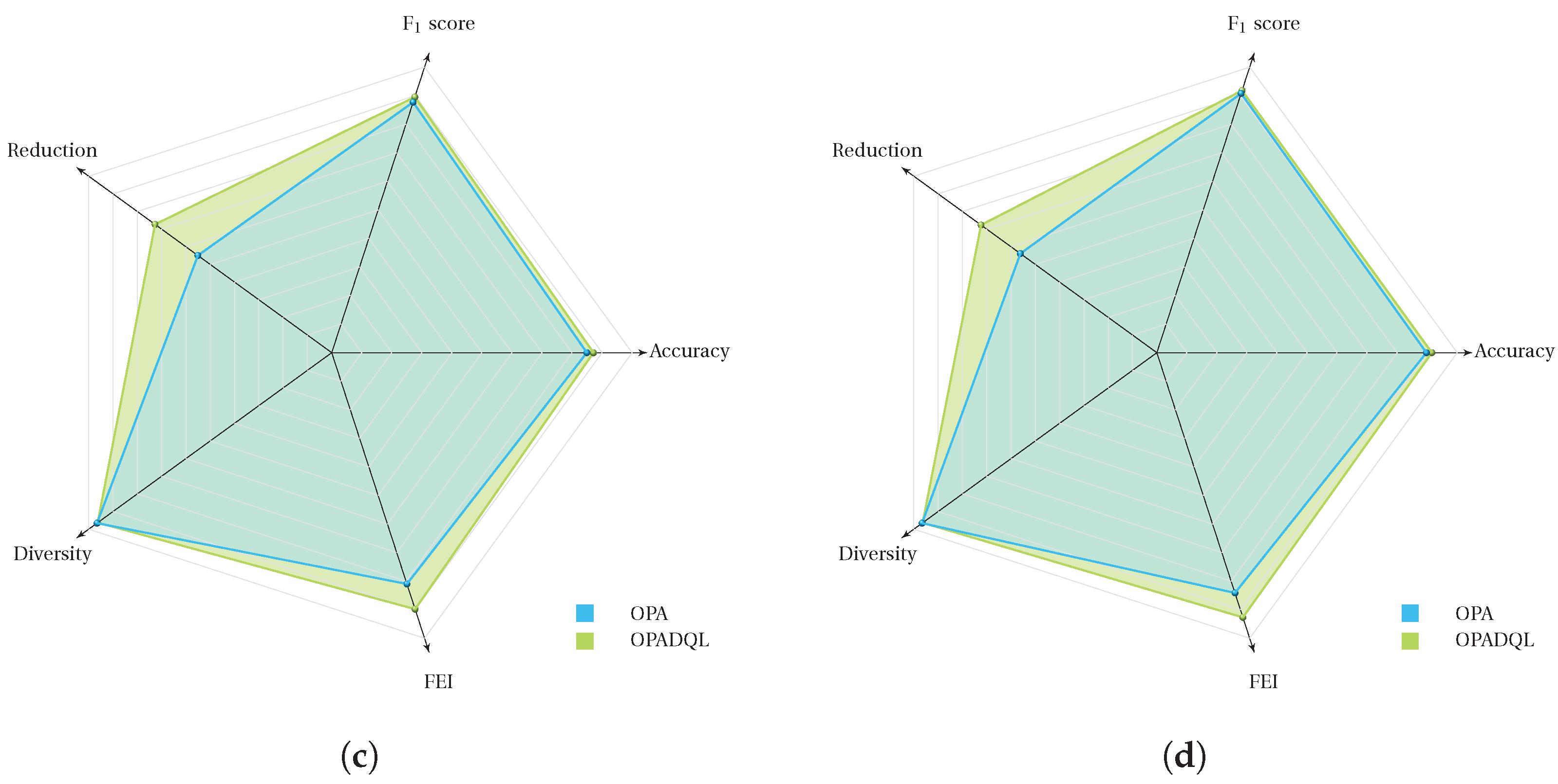
Table 1.
Parameter setting.
| Parameter | Value or Description |
|---|---|
| q | 0.9 |
| a | Closer to 1 |
| b | Random |
| d | Closer to 1 |
| F | Close to 2 |
| S | 10 |
| Maximum iterations | 100 |
| State size | 5 |
| Action size | 40 |
| Neurons per layer | 24 |
| Activation | ReLU (layers), Linear (final layer) |
| Loss function | Huber |
| Optimizer | RMSprop with a learning rate of |
| Epsilon | Starts at 1.0, decays to |
| Network update | Every 50 training steps |
| Initial parameters | Randomly generated in range [0, 1] |
| Binarization threshold () | Random value uniformly distributed [0, 1] |
Table 2.
Comparative analysis of algorithms’ performance: OPA vs. OPADQL for DT and RF.
| Metrics | DT | RF | |||||
|---|---|---|---|---|---|---|---|
| n/o | OPA | OPADQL | n/o | OPA | OPADQL | ||
| score | 0.7911 | 0.8242 | 0.8250 | 0.9154 | 0.9165 | 0.9186 | |
| 0.7753 | 0.7601 | 0.7936 | 0.8671 | 0.8921 | 0.9087 | ||
| 0.7829 | 0.7845 | 0.8093 | 0.8956 | 0.9110 | 0.9124 | ||
| 0.0037 | 0.0062 | 0.0133 | 0.0016 | 0.0045 | 0.0137 | ||
| 0.7835 | 0.7851 | 0.8087 | 0.9002 | 0.9107 | 0.9120 | ||
| 0.0045 | 0.0070 | 0.0209 | 0.0023 | 0.0062 | 0.0194 | ||
| Accuracy | 0.7408 | 0.7886 | 0.9035 | 0.8978 | 0.8989 | 0.9035 | |
| 0.7207 | 0.7225 | 0.7432 | 0.8897 | 0.8342 | 0.8673 | ||
| 0.7299 | 0.7307 | 0.8921 | 0.8731 | 0.8921 | 0.8943 | ||
| 0.0047 | 0.0071 | 0.0159 | 0.0021 | 0.0071 | 0.0176 | ||
| 0.7304 | 0.7328 | 0.8922 | 0.8782 | 0.8922 | 0.8940 | ||
| 0.0065 | 0.0091 | 0.0240 | 0.0035 | 0.0108 | 0.0257 | ||
| Diversity | n/a | 0.9647 | 0.9691 | n/a | 0.9666 | 0.9692 | |
| n/a | 0.9576 | 0.9116 | n/a | 0.9420 | 0.9405 | ||
| n/a | 0.9611 | 0.9659 | n/a | 0.9647 | 0.9616 | ||
| n/a | 0.0096 | 0.0019 | n/a | 0.0096 | 0.0053 | ||
| n/a | 0.9636 | 0.9663 | n/a | 0.9663 | 0.9637 | ||
| n/a | 0.0003 | 0.0003 | n/a | 0.0014 | 0.0003 | ||
| Reduction | n/a | 0.6043 | 0.9645 | n/a | 0.6043 | 0.8014 | |
| n/a | 0.5026 | 0.6099 | n/a | 0.5133 | 0.5390 | ||
| n/a | 0.5378 | 0.6811 | n/a | 0.5575 | 0.6622 | ||
| n/a | 0.0234 | 0.7328 | n/a | 0.0259 | 0.8782 | ||
| n/a | 0.5957 | 0.6738 | n/a | 0.5615 | 0.6773 | ||
| n/a | 0.0321 | 0.0390 | n/a | 0.0401 | 0.1170 | ||
| FEI | n/a | 0.7800 | 0.8991 | n/a | 0.8432 | 0.9259 | |
| n/a | 0.7646 | 0.7992 | n/a | 0.8154 | 0.8615 | ||
| n/a | 0.7710 | 0.8293 | n/a | 0.8300 | 0.8881 | ||
| n/a | 0.0042 | 0.0117 | n/a | 0.0059 | 0.0160 | ||
| n/a | 0.0770 | 0.8276 | n/a | 0.8311 | 0.8871 | ||
| n/a | 0.0065 | 0.0178 | n/a | 0.0082 | 0.0265 | ||
Table 3.
Comparative analysis of algorithms’ performance: OPA vs. OPADQL for SVM and ERT.
| Metrics | SVM | ERT | |||||
|---|---|---|---|---|---|---|---|
| n/o | OPA | OPADQL | n/o | OPA | OPADQL | ||
| score | 0.8841 | 0.8843 | 0.9155 | 0.9168 | 0.9180 | 0.9228 | |
| 0.8841 | 0.8644 | 0.8645 | 0.9108 | 0.8392 | 0.9048 | ||
| 0.8841 | 0.8766 | 0.8919 | 0.9145 | 0.8946 | 0.9153 | ||
| 0.0000 | 0.0051 | 0.0129 | 0.0014 | 0.0048 | 0.0177 | ||
| 0.8841 | 0.8771 | 0.8954 | 0.9147 | 0.8974 | 0.9155 | ||
| 0.0000 | 0.0082 | 0.0175 | 0.0021 | 0.0066 | 0.0234 | ||
| Accuracy | 0.8565 | 0.8594 | 0.8966 | 0.8975 | 0.9013 | 0.9078 | |
| 0.8565 | 0.8328 | 0.8344 | 0.8910 | 0.8023 | 0.8826 | ||
| 0.8565 | 0.8488 | 0.8682 | 0.8951 | 0.8710 | 0.8973 | ||
| 0.0000 | 0.0069 | 0.0158 | 0.0016 | 0.0066 | 0.0218 | ||
| 0.8565 | 0.8493 | 0.8713 | 0.8953 | 0.8755 | 0.8976 | ||
| 0.0000 | 0.0106 | 0.0215 | 0.0026 | 0.0091 | 0.0276 | ||
| Diversity | n/a | 0.9671 | 0.9638 | n/a | 0.9637 | 0.9661 | |
| n/a | 0.9525 | 0.9306 | n/a | 0.9326 | 0.9557 | ||
| n/a | 0.9650 | 0.9593 | n/a | 0.9629 | 0.9642 | ||
| n/a | 0.0053 | 0.0088 | n/a | 0.0015 | 0.0061 | ||
| n/a | 0.9658 | 0.9631 | n/a | 0.9634 | 0.9659 | ||
| n/a | 0.0003 | 0.0041 | n/a | 0.0010 | 0.0010 | ||
| Reduction | n/a | 0.5829 | 0.8014 | n/a | 0.6043 | 0.8014 | |
| n/a | 0.5133 | 0.5673 | n/a | 0.5133 | 0.6312 | ||
| n/a | 0.5519 | 0.7026 | n/a | 0.5565 | 0.7272 | ||
| n/a | 0.0190 | 0.8713 | n/a | 0.0214 | 0.8755 | ||
| n/a | 0.5508 | 0.7270 | n/a | 0.5615 | 0.7234 | ||
| n/a | 0.0254 | 0.0975 | n/a | 0.0254 | 0.0408 | ||
| FEI | n/a | 0.8220 | 0.9342 | n/a | 0.8434 | 0.9265 | |
| n/a | 0.8014 | 0.8650 | n/a | 0.8237 | 0.8798 | ||
| n/a | 0.8105 | 0.8955 | n/a | 0.8333 | 0.9039 | ||
| n/a | 0.0048 | 0.0168 | n/a | 0.0048 | 0.0110 | ||
| n/a | 0.8100 | 0.8981 | n/a | 0.8333 | 0.9043 | ||
| n/a | 0.0046 | 0.0223 | n/a | 0.0059 | 0.0139 | ||
Table 4.
p-values obtained from Wilcoxon–Mann–Whitney Test.
| Metrics | OPADQL v/s OPA | |||
|---|---|---|---|---|
| DT | RF | SVM | ERT | |
| Accuracy | ||||
| Diversity | sws | sws | ||
| Reduction | ||||
| FEI | ||||
Table 5.
OPADQL for DT and RF vs. state-of-the-art algorithms.
| Metrics | Random | GA | PSO | BAT | BH | GWO | GEO | RSA | OPADQL | |
|---|---|---|---|---|---|---|---|---|---|---|
| Decision Tree | ||||||||||
| score | 0.8191 | 0.8085 | 0.8106 | 0.8126 | 0.8147 | 0.8168 | 0.8137 | 0.8151 | 0.8250 | |
| 0.7781 | 0.7777 | 0.7797 | 0.7817 | 0.7837 | 0.7857 | 0.7811 | 0.7827 | 0.7936 | ||
| 0.7929 | 0.7931 | 0.7951 | 0.7972 | 0.7992 | 0.8012 | 0.7965 | 0.7981 | 0.8093 | ||
| 0.0011 | 0.0049 | 0.0069 | 0.0049 | 0.0059 | 0.0109 | 0.0058 | 0.0067 | 0.0133 | ||
| 0.7935 | 0.7931 | 0.7951 | 0.7971 | 0.7991 | 0.8011 | 0.7965 | 0.7980 | 0.8087 | ||
| 0.0011 | 0.0207 | 0.0177 | 0.0027 | 0.0201 | 0.0200 | 0.0137 | 0.0146 | 0.0209 | ||
| Accuracy | 0.7720 | 0.8854 | 0.8877 | 0.8899 | 0.8922 | 0.8945 | 0.8703 | 0.8744 | 0.9035 | |
| 0.7107 | 0.7283 | 0.7302 | 0.7321 | 0.7339 | 0.7358 | 0.7285 | 0.7303 | 0.7432 | ||
| 0.7499 | 0.8743 | 0.8765 | 0.8787 | 0.8809 | 0.8832 | 0.8573 | 0.8616 | 0.8921 | ||
| 0.0117 | 0.0049 | 0.0049 | 0.0049 | 0.0049 | 0.0049 | 0.0060 | 0.0073 | 0.0159 | ||
| 0.7463 | 0.8741 | 0.8761 | 0.8791 | 0.8811 | 0.8830 | 0.8566 | 0.8611 | 0.8922 | ||
| 0.0115 | 0.0215 | 0.0211 | 0.0225 | 0.0235 | 0.0217 | 0.0203 | 0.0208 | 0.0240 | ||
| Diversity | n/a | 0.9645 | 0.9650 | 0.9701 | 0.9748 | 0.9698 | 0.9689 | 0.9699 | 0.9691 | |
| n/a | 0.9574 | 0.9575 | 0.9576 | 0.9577 | 0.9578 | 0.9499 | 0.9509 | 0.9116 | ||
| n/a | 0.9600 | 0.9611 | 0.9612 | 0.9613 | 0.9614 | 0.9618 | 0.9628 | 0.9659 | ||
| n/a | 0.0048 | 0.0049 | 0.0052 | 0.0053 | 0.0052 | 0.0045 | 0.0055 | 0.0019 | ||
| n/a | 0.9590 | 0.9600 | 0.9615 | 0.9611 | 0.9612 | 0.9615 | 0.9625 | 0.9663 | ||
| n/a | 0.0048 | 0.0049 | 0.0050 | 0.0051 | 0.0052 | 0.0042 | 0.0052 | 0.0003 | ||
| Reduction | 0.5634 | 0.6041 | 0.6042 | 0.6043 | 0.6044 | 0.7045 | 0.6142 | 0.6579 | 0.9645 | |
| 0.4564 | 0.5024 | 0.5025 | 0.5026 | 0.5027 | 0.5928 | 0.5099 | 0.5224 | 0.6099 | ||
| 0.4873 | 0.5376 | 0.5377 | 0.5378 | 0.5379 | 0.6380 | 0.5460 | 0.5629 | 0.6811 | ||
| 0.0375 | 0.0276 | 0.0278 | 0.0277 | 0.0279 | 0.0279 | 0.0294 | 0.1173 | 0.7328 | ||
| 0.4863 | 0.5370 | 0.5371 | 0.5371 | 0.5373 | 0.6373 | 0.5454 | 0.5614 | 0.6738 | ||
| 0.0144 | 0.0276 | 0.0277 | 0.0278 | 0.0279 | 0.0280 | 0.0256 | 0.0272 | 0.0390 | ||
| FEI | 0.7200 | 0.8570 | 0.7756 | 0.8100 | 0.7890 | 0.8700 | 0.8036 | 0.8155 | 0.8991 | |
| 0.6320 | 0.7900 | 0.7100 | 0.7110 | 0.6915 | 0.7950 | 0.7216 | 0.7313 | 0.7992 | ||
| 0.6767 | 0.8200 | 0.7400 | 0.7710 | 0.7215 | 0.8250 | 0.7590 | 0.7678 | 0.8293 | ||
| 0.0204 | 0.0100 | 0.0102 | 0.0104 | 0.0106 | 0.0110 | 0.0121 | 0.0121 | 0.0117 | ||
| 0.6747 | 0.8230 | 0.7354 | 0.7340 | 0.7545 | 0.8270 | 0.7581 | 0.7668 | 0.8276 | ||
| 0.0276 | 0.0160 | 0.0162 | 0.0164 | 0.0166 | 0.0170 | 0.0183 | 0.0182 | 0.0178 | ||
| Random Forest | ||||||||||
| score | 0.8915 | 0.9002 | 0.9025 | 0.9048 | 0.9071 | 0.9094 | 0.9026 | 0.9046 | 0.9186 | |
| 0.8671 | 0.8905 | 0.8928 | 0.8951 | 0.8973 | 0.8996 | 0.8904 | 0.8927 | 0.9087 | ||
| 0.8956 | 0.8942 | 0.8964 | 0.8987 | 0.901 | 0.9033 | 0.8982 | 0.9000 | 0.9124 | ||
| 0.0016 | 0.0213 | 0.0213 | 0.0213 | 0.0213 | 0.0213 | 0.0180 | 0.0175 | 0.0137 | ||
| 0.8802 | 0.8940 | 0.8960 | 0.8990 | 0.9010 | 0.9030 | 0.8955 | 0.8976 | 0.9120 | ||
| 0.0023 | 0.0173 | 0.0183 | 0.0131 | 0.0013 | 0.0113 | 0.0106 | 0.0117 | 0.0194 | ||
| Accuracy | 0.9001 | 0.8854 | 0.8877 | 0.8899 | 0.8922 | 0.8945 | 0.8916 | 0.8931 | 0.9035 | |
| 0.8897 | 0.8556 | 0.8521 | 0.8543 | 0.8565 | 0.8586 | 0.8611 | 0.8619 | 0.8673 | ||
| 0.8731 | 0.8764 | 0.8786 | 0.8809 | 0.8831 | 0.8854 | 0.8796 | 0.8814 | 0.8943 | ||
| 0.0021 | 0.0213 | 0.0213 | 0.0213 | 0.0213 | 0.0213 | 0.0181 | 0.0180 | 0.0176 | ||
| 0.8782 | 0.8760 | 0.8790 | 0.8810 | 0.8830 | 0.8850 | 0.8804 | 0.8821 | 0.8940 | ||
| 0.0015 | 0.0213 | 0.0225 | 0.0215 | 0.0213 | 0.0223 | 0.0184 | 0.0193 | 0.0257 | ||
| Diversity | n/a | 0.9725 | 0.9701 | 0.9766 | 0.9699 | 0.9749 | 0.9728 | 0.9723 | 0.9692 | |
| n/a | 0.9574 | 0.9575 | 0.9576 | 0.9577 | 0.9578 | 0.9576 | 0.9552 | 0.9405 | ||
| n/a | 0.9710 | 0.9654 | 0.9681 | 0.9613 | 0.9740 | 0.9680 | 0.9671 | 0.9616 | ||
| n/a | 0.0048 | 0.0049 | 0.0050 | 0.0051 | 0.0052 | 0.0050 | 0.0050 | 0.0053 | ||
| n/a | 0.9711 | 0.9610 | 0.9610 | 0.9610 | 0.9610 | 0.9630 | 0.9631 | 0.9637 | ||
| n/a | 0.0048 | 0.0059 | 0.0050 | 0.0051 | 0.0052 | 0.0052 | 0.0045 | 0.0003 | ||
| Reduction | 0.5469 | 0.6041 | 0.6242 | 0.6143 | 0.6344 | 0.7045 | 0.6214 | 0.6439 | 0.8014 | |
| 0.4475 | 0.5024 | 0.5025 | 0.5026 | 0.5027 | 0.5028 | 0.4934 | 0.4991 | 0.5390 | ||
| 0.4948 | 0.5376 | 0.5377 | 0.5578 | 0.5479 | 0.6380 | 0.5523 | 0.5660 | 0.6622 | ||
| 0.0269 | 0.0276 | 0.0277 | 0.0278 | 0.0289 | 0.0280 | 0.0278 | 0.1341 | 0.8782 | ||
| 0.4917 | 0.5378 | 0.5485 | 0.5599 | 0.5364 | 0.6370 | 0.5519 | 0.5676 | 0.6773 | ||
| 0.0469 | 0.0276 | 0.0277 | 0.0278 | 0.0279 | 0.0280 | 0.0310 | 0.0417 | 0.1170 | ||
| FEI | 0.7823 | 0.8000 | 0.7892 | 0.7821 | 0.8021 | 0.8823 | 0.8063 | 0.8213 | 0.9259 | |
| 0.7257 | 0.6250 | 0.5355 | 0.6160 | 0.7065 | 0.8300 | 0.6731 | 0.6967 | 0.8615 | ||
| 0.7567 | 0.7010 | 0.6635 | 0.7040 | 0.7445 | 0.8660 | 0.7393 | 0.7579 | 0.8881 | ||
| 0.0150 | 0.0140 | 0.0142 | 0.0144 | 0.0146 | 0.0150 | 0.0145 | 0.0147 | 0.0160 | ||
| 0.7564 | 0.7050 | 0.6655 | 0.7060 | 0.7465 | 0.8670 | 0.7411 | 0.7593 | 0.8871 | ||
| 0.0257 | 0.0257 | 0.0252 | 0.0254 | 0.0056 | 0.0260 | 0.0223 | 0.0228 | 0.0265 | ||
Table 6.
OPADQL for SVM and ERT vs. state-of-the-art algorithms.
| Metrics | Random | GA | PSO | BAT | BH | GWO | GEO | RSA | OPADQL | |
|---|---|---|---|---|---|---|---|---|---|---|
| Support Vector Machine | ||||||||||
| score | 0.8874 | 0.9052 | 0.9073 | 0.9094 | 0.9115 | 0.9170 | 0.9063 | 0.9075 | 0.9155 | |
| 0.8485 | 0.8550 | 0.8560 | 0.8570 | 0.8580 | 0.8660 | 0.8567 | 0.8577 | 0.8645 | ||
| 0.8666 | 0.8890 | 0.8895 | 0.8900 | 0.8905 | 0.8930 | 0.8864 | 0.8871 | 0.8919 | ||
| 0.0087 | 0.0125 | 0.0126 | 0.0127 | 0.0128 | 0.0130 | 0.0121 | 0.0122 | 0.0131 | ||
| 0.8664 | 0.8890 | 0.8895 | 0.8900 | 0.8905 | 0.8978 | 0.8872 | 0.8882 | 0.8954 | ||
| 0.0098 | 0.0160 | 0.0162 | 0.0164 | 0.0166 | 0.0178 | 0.0155 | 0.0157 | 0.0175 | ||
| Accuracy | 0.8615 | 0.8860 | 0.8865 | 0.8870 | 0.8875 | 0.8994 | 0.8847 | 0.8861 | 0.8966 | |
| 0.8144 | 0.8250 | 0.8260 | 0.8270 | 0.8280 | 0.8290 | 0.8249 | 0.8261 | 0.8344 | ||
| 0.8361 | 0.8610 | 0.8615 | 0.8620 | 0.8625 | 0.8692 | 0.8587 | 0.8599 | 0.8682 | ||
| 0.0113 | 0.0145 | 0.0146 | 0.0147 | 0.0148 | 0.0149 | 0.0141 | 0.0143 | 0.0158 | ||
| 0.8360 | 0.8610 | 0.8615 | 0.8620 | 0.8625 | 0.8630 | 0.8577 | 0.8594 | 0.8713 | ||
| 0.0131 | 0.0200 | 0.0002 | 0.0204 | 0.0006 | 0.0308 | 0.0142 | 0.0151 | 0.0215 | ||
| Diversity | n/a | 0.9636 | 0.9637 | 0.9638 | 0.9639 | 0.9640 | 0.9638 | 0.9638 | 0.9638 | |
| n/a | 0.9304 | 0.9305 | 0.9306 | 0.9307 | 0.9308 | 0.9306 | 0.9306 | 0.9306 | ||
| n/a | 0.9591 | 0.9592 | 0.9593 | 0.9594 | 0.9595 | 0.9593 | 0.9593 | 0.9593 | ||
| n/a | 0.0086 | 0.0087 | 0.0088 | 0.0089 | 0.0090 | 0.0088 | 0.0088 | 0.0088 | ||
| n/a | 0.9591 | 0.9592 | 0.9593 | 0.9594 | 0.9595 | 0.9593 | 0.9598 | 0.9631 | ||
| n/a | 0.0038 | 0.0039 | 0.0040 | 0.0041 | 0.0042 | 0.0040 | 0.0040 | 0.0041 | ||
| Reduction | 0.5524 | 0.6812 | 0.4813 | 0.5814 | 0.6715 | 0.7916 | 0.6266 | 0.6484 | 0.8014 | |
| 0.4088 | 0.5571 | 0.4072 | 0.5573 | 0.5574 | 0.5575 | 0.5076 | 0.5150 | 0.5673 | ||
| 0.4987 | 0.6024 | 0.4525 | 0.6926 | 0.5927 | 0.6928 | 0.5886 | 0.6029 | 0.7026 | ||
| 0.0350 | 0.8608 | 0.8609 | 0.8610 | 0.8611 | 0.8612 | 0.7233 | 0.7418 | 0.8713 | ||
| 0.5027 | 0.6024 | 0.4625 | 0.6926 | 0.5927 | 0.6928 | 0.5910 | 0.6080 | 0.7270 | ||
| 0.0441 | 0.0950 | 0.0435 | 0.0252 | 0.0053 | 0.0954 | 0.0514 | 0.0572 | 0.0975 | ||
| FEI | 0.5524 | 0.6812 | 0.4813 | 0.5814 | 0.6715 | 0.7916 | 0.6266 | 0.6484 | 0.8014 | |
| 0.4088 | 0.5571 | 0.4072 | 0.5573 | 0.5574 | 0.5575 | 0.5076 | 0.5150 | 0.5673 | ||
| 0.4987 | 0.6024 | 0.4525 | 0.6926 | 0.5927 | 0.6928 | 0.5886 | 0.6029 | 0.7026 | ||
| 0.0350 | 0.8608 | 0.8609 | 0.8610 | 0.8611 | 0.8612 | 0.7233 | 0.7418 | 0.8713 | ||
| 0.5027 | 0.6024 | 0.4625 | 0.6926 | 0.5927 | 0.6928 | 0.5910 | 0.6080 | 0.7270 | ||
| 0.0441 | 0.0950 | 0.0435 | 0.0252 | 0.0053 | 0.0954 | 0.0514 | 0.0572 | 0.0975 | ||
| Extremely Randomized Trees | ||||||||||
| score | 0.9121 | 0.9201 | 0.9202 | 0.9203 | 0.9204 | 0.9240 | 0.9195 | 0.9199 | 0.9228 | |
| 0.8823 | 0.9020 | 0.9021 | 0.9022 | 0.9023 | 0.9060 | 0.8995 | 0.9001 | 0.9048 | ||
| 0.9023 | 0.9140 | 0.9141 | 0.9142 | 0.9143 | 0.9160 | 0.9125 | 0.9128 | 0.9153 | ||
| 0.0014 | 0.0172 | 0.0173 | 0.0174 | 0.0175 | 0.0179 | 0.0148 | 0.0152 | 0.0177 | ||
| 0.8947 | 0.9140 | 0.9141 | 0.9142 | 0.9143 | 0.9160 | 0.9112 | 0.9118 | 0.9155 | ||
| 0.0021 | 0.0225 | 0.0226 | 0.0227 | 0.0228 | 0.0235 | 0.0194 | 0.0199 | 0.0234 | ||
| Accuracy | 0.9052 | 0.9050 | 0.9055 | 0.9060 | 0.9065 | 0.9070 | 0.9059 | 0.9061 | 0.9078 | |
| 0.8620 | 0.8800 | 0.8805 | 0.8810 | 0.8815 | 0.8820 | 0.8778 | 0.8784 | 0.8826 | ||
| 0.8806 | 0.8950 | 0.8955 | 0.8960 | 0.8965 | 0.8970 | 0.8934 | 0.8962 | 0.8973 | ||
| 0.0016 | 0.0205 | 0.0206 | 0.0207 | 0.0208 | 0.0209 | 0.0175 | 0.0181 | 0.0218 | ||
| 0.8953 | 0.8950 | 0.8955 | 0.8960 | 0.8965 | 0.8970 | 0.8959 | 0.8961 | 0.8976 | ||
| 0.0026 | 0.0260 | 0.0262 | 0.0264 | 0.0266 | 0.0268 | 0.0224 | 0.0231 | 0.0276 | ||
| Diversity | n/a | 0.9659 | 0.9660 | 0.9661 | 0.9662 | 0.9663 | 0.9665 | 0.9664 | 0.9661 | |
| n/a | 0.9555 | 0.9556 | 0.9557 | 0.9558 | 0.9559 | 0.9561 | 0.9563 | 0.9557 | ||
| n/a | 0.9640 | 0.9641 | 0.9642 | 0.9643 | 0.9644 | 0.9646 | 0.9645 | 0.9642 | ||
| n/a | 0.0062 | 0.0061 | 0.0062 | 0.0063 | 0.0064 | 0.0066 | 0.0065 | 0.0061 | ||
| n/a | 0.9640 | 0.9641 | 0.9642 | 0.9643 | 0.9644 | 0.9647 | 0.9646 | 0.9659 | ||
| n/a | 0.0008 | 0.0009 | 0.0010 | 0.0011 | 0.0012 | 0.0014 | 0.0013 | 0.0010 | ||
| Reduction | 0.5414 | 0.7912 | 0.7913 | 0.7914 | 0.7915 | 0.7916 | 0.7497 | 0.7562 | 0.8014 | |
| 0.4530 | 0.6210 | 0.6211 | 0.6212 | 0.6213 | 0.6214 | 0.5932 | 0.5979 | 0.6312 | ||
| 0.4983 | 0.7170 | 0.7171 | 0.7172 | 0.7173 | 0.7174 | 0.6807 | 0.6865 | 0.7272 | ||
| 0.0270 | 0.8650 | 0.8651 | 0.8652 | 0.8653 | 0.8654 | 0.7255 | 0.7443 | 0.8755 | ||
| 0.5000 | 0.7170 | 0.7171 | 0.7172 | 0.7173 | 0.7174 | 0.681 | 0.6863 | 0.7234 | ||
| 0.0359 | 0.0395 | 0.0396 | 0.0397 | 0.0398 | 0.0399 | 0.0391 | 0.0393 | 0.0408 | ||
| FEI | 0.7894 | 0.8752 | 0.8053 | 0.8125 | 0.8257 | 0.9059 | 0.8357 | 0.8470 | 0.9265 | |
| 0.7334 | 0.8087 | 0.6888 | 0.7189 | 0.7590 | 0.8091 | 0.7530 | 0.7688 | 0.8798 | ||
| 0.7604 | 0.84027 | 0.7228 | 0.7630 | 0.7731 | 0.8433 | 0.7838 | 0.7988 | 0.9039 | ||
| 0.0156 | 0.0106 | 0.0107 | 0.0108 | 0.0109 | 0.0110 | 0.0116 | 0.0115 | 0.0110 | ||
| 0.7691 | 0.8427 | 0.7328 | 0.7630 | 0.7701 | 0.8333 | 0.7852 | 0.8001 | 0.9043 | ||
| 0.0020 | 0.0035 | 0.0136 | 0.0107 | 0.0108 | 0.0039 | 0.0074 | 0.0082 | 0.0139 | ||
Disclaimer/Publisher’s Note: The statements, opinions and data contained in all publications are solely those of the individual author(s) and contributor(s) and not of MDPI and/or the editor(s). MDPI and/or the editor(s) disclaim responsibility for any injury to people or property resulting from any ideas, methods, instructions or products referred to in the content. |
© 2024 by the authors. Licensee MDPI, Basel, Switzerland. This article is an open access article distributed under the terms and conditions of the Creative Commons Attribution (CC BY) license (https://creativecommons.org/licenses/by/4.0/).
Share and Cite
MDPI and ACS Style
Olivares, R.; Ravelo, C.; Soto, R.; Crawford, B. Escaping Stagnation through Improved Orca Predator Algorithm with Deep Reinforcement Learning for Feature Selection. Mathematics 2024, 12, 1249. https://doi.org/10.3390/math12081249
AMA Style
Olivares R, Ravelo C, Soto R, Crawford B. Escaping Stagnation through Improved Orca Predator Algorithm with Deep Reinforcement Learning for Feature Selection. Mathematics. 2024; 12(8):1249. https://doi.org/10.3390/math12081249
Chicago/Turabian StyleOlivares, Rodrigo, Camilo Ravelo, Ricardo Soto, and Broderick Crawford. 2024. "Escaping Stagnation through Improved Orca Predator Algorithm with Deep Reinforcement Learning for Feature Selection" Mathematics 12, no. 8: 1249. https://doi.org/10.3390/math12081249
Note that from the first issue of 2016, this journal uses article numbers instead of page numbers. See further details here.