A Nonlinear ODE Model for a Consumeristic Society

Abstract

In this paper, we introduce an ODE system to model the interaction between natural resources and human exploitation in a rich consumeristic society. In this model, the rate of change in population depends on wealth per capita, and the rate of consumption has a quadratic growth with respect to population and wealth. We distinguish between renewable and non-renewable resources, and we introduce a replenishment term for non-renewable resources. We first obtain some information on the asymptotic behavior of wealth and population, then we compute all system equilibria and study their stability when the resource exploitation parameter is low. Some numerical simulations confirm the theoretical results and suggest directions for future research.

1. Introduction

In this paper, we study a model of interactions between society and nature, whose original inspiration goes back to the HANDY model introduced in [1] (see also [2,3]). The original HANDY model is a set of four differential equations whose variables are natural resources, wealth produced by human work, and population, split in the two classes of Commoner and Elite. Using computer simulations, the paper [1] shows different possibilities for the evolution of society, including collapse. It is a simple model that seems to allow a rich panel of behavior, so it attracted attention, and several papers have been devoted to its exploration, trying to generalize the original idea in several, different directions. In [4], the HANDY model is studied using a Lyapunov-type analysis. The authors give an interesting mathematical generalization of the original model, proving that a set of qualitative hypotheses on the state variables implies collapse, even without assuming that the functions involved are solutions of a system of differential equations. In [5], the authors on one hand simplify the HANDY model, dropping the division of population in two classes, and on the other hand use general nonlinear functions to describe the equations involving the state variables, which are “population”, “resources”, and “reserves”. Because of the generality of their model, they are able to treat different sets of hypotheses on the interactions between the state variables. More recently, Tonnelier [6] presented a clearer rewrite of the HANDY model and studied its dynamics using bifurcation techniques and focusing on the influence of two parameters: the nature depletion rate and the inequality factor. All these works, after the mathematical analysis, give several kinds of numerical simulations, exploring the actual dynamics of the system for some fixed values of the parameters. Computational techniques applied to the HANDY model are the main subject of [7].

Our work is more directly linked to some ideas introduced in [8,9]. In [8], various developments of the original model are introduced, including, among other aspects, the division of natural resources into renewable and non-renewable categories. This idea has been developed in the paper [9], where some general results are obtained and again numerical simulations show different possibilities for the evolution of society. In [9] the dynamics of non-renewable resources is given by the following equation

$$\frac{d{y}_n}{dt}=-{\delta }_n{x}_c{y}_n,$$

where $y_n$ is the variable for the non-renewable resources, $x_c$ is the Commoner population and ${\delta }_n>0$ is a parameter. Clearly, this equation translates the idea of a given amount and an irreversible depletion of $y_n$. In our previous work [2], we have pursued this idea but we have introduced a replenishment term for non-renewable resources. This is due to the optimistic argument, which is often used in public debate on these subjects, that human ingenuity and scientific progress can substitute depleted resources with new ones. The term of replenishment that we have added is given by

$$k\frac{xw}{xw+1}z.$$

This term depends on $xw$, where x represents the population, w represents wealth, z is the level of non-renewable resources, and k is a constant. Hence, the dynamics of non-renewable resources z in [2] is given by

$$z^{\prime }=k\frac{xw}{xw+1}z-\delta zx,$$

The replenishment term is obtained from a function $\frac{t}{t+1}$ which, in population dynamics, is a Holling II-type function (see [10], p. 25 and passim), used to model saturation effects. The equation above states that the replenishment is possible but cannot be above a level k, and we can call this an hypothesis of “moderate optimism”. Another characteristic of [2] is that we dropped the distinction between Commoner and Elite, so we obtained a model with four variables, which are population, renewable and non-renewable resources, wealth. In [2], we obtained all the critical points of the system, and we studied their stability. In the final section of [2], numerical simulations support the theoretical results and also suggest the possibility, not yet treated in a rigorous way, of periodic orbits and chaotic dynamics.

The present paper originated from the attempt to adapt the HANDY model to contemporary, rich, consumeristic societies (like contemporary Western countries). Indeed, the HANDY model seems to be a very nice and simple way to treat the interaction of nature and society for a large class of historical societies, but, in our opinion, it has some serious flaws when dealing with contemporary, rich, consumeristic societies. The main one is probably the fact that in the original model, the birth rate is constant and the death rate decays when wealth increases, leading to the conclusion that a wealthy society should have a strong population growth. This is definitely not true in contemporary Western societies, and the reason for this is due to the fact that birth rate is not constant, and indeed, in most contemporary rich societies, it is falling. Hence, to study rich, contemporary societies, it seems necessary to overcome the HANDY model used in the papers quoted above (including our previous paper [2]) and to introduce new ideas. This is what we do in the present paper. Firstly, we introduce an equation for population dynamics which is different from that of HANDY model, and it is as follows

$$x^{\prime }=-cx+d\frac{\mu xw}{w^2+{\mu }^2{x}^2}x.$$

Here, x is the population and w the wealth. In this equation we have a negative term $-cx$, which is balanced by the term

$$d\frac{\mu xw}{w^2+{\mu }^2{x}^2}x=d\frac{\frac{w}{\mu x}}{{\left(\frac{w}{\mu x}\right)}^2+1}x,$$

depending on the wealth per capita $w/x$ via a constant $\mu$. When $w/\mu x$ is very small or very large, the positive term is small and the population falls. In an intermediate region, the population grows. This seems to better fit the recent history of rich countries.

Another difference compared to the HANDY model (and to [2]) is that in previous works the depletion of natural resources depends on the population, while it seems reasonable that in a consumeristic society it should depend more on wealth than on population. Hence, a first idea should be to substitute population with wealth (x with w) in the depletion terms, giving rise to quadratic terms $w^2$. We will pursue this idea in a forthcoming paper. In the present paper, however, we are interested in preserving some influence of population on consumption of natural resources, so we introduce the function $m=m(x,w)=max\{x,w\}$ and we substitute x with m in the depletion terms. We notice also that the consumption term in the equation for $w^{\prime }$ in [2], which is given by $s\left[x-\frac{1}{\rho }{(\rho x-w)}^{+}\right],$ has a linear growth, while here, to model a consumeristic society, we use a quadratic term $m(x,w)w$, where the consumption is led mostly by wealth.

Summing up all these ideas, and applying some standard rescaling, the model we are going to study in the present paper is the following

$$\left\{\begin{array}{cc}\hfill x^{\prime }& =-cx+d\frac{\mu xw}{w^2+{\mu }^2{x}^2}x\hfill \\ \hfill y^{\prime }& =\gamma y(\lambda -y)-\delta ym(x,w)\hfill \\ \hfill z^{\prime }& =k\frac{m(x,w)w}{m(x,w)w+1}z-\delta zm(x,w)\hfill \\ \hfill w^{\prime }& =\delta ym(x,w)+\delta zm(x,w)-\sigma m(x,w)w.\hfill \end{array}\right.$$

(1)

where x is the population, y and z are the renewable and non-renewable resources, w is the wealth. As we said above, $m(x,w)=max\{x,w\}=\frac{1}{2}(x+w+|x-w\left|\right)$.

We underline that, because of the changes that have been explained above, the present model can no longer be considered a HANDY-type model, as it was the model of our previous work [2].

To start the work with (1) we need some assumptions on the parameters. Firstly, we assume $d>2c$, which is necessary to have a positive growth of x for some range of $\frac{w}{\mu x}$. Indeed, if $d\le 2c$, then it is

$$-c+d\frac{\mu xw}{w^2+{\mu }^2{x}^2}\le 0,$$

for any value of $x,w$, hence it is always $x^{\prime }\le 0$, making the model less interesting. We also assume $\mu >1$, which means that the ratio $w/\mu x$ becomes large only when w is larger than x, and this implies that the negative effect on the population growth of the increasing wealth becomes relevant only for large values of wealth per capita. We also assume $\mu \ne \frac{d+\sqrt{d^2-4c^2}}{2c}$, which is just a technical assumption that we will drop in a forthcoming paper. We remark that in (1), the depletion rates for renewable and non-renewable resources are equal. This is a simplifying assumption that we hope to drop in future research. In our previous paper [2], numerical simulations seemed to suggest that the dynamics do not change too much taking different values for the depletion rates. In Section 7, some simulations show a different dependence of the dynamics on the two depletion rates (which are labeled ${\delta }_1$ and ${\delta }_2$), and this seems an interesting topic for future research.

The present paper is organized as follows. After the introduction, in Section 2 we obtain general results for the existence and positivity of the solutions, as well as results on their asymptotic behavior. In particular, we prove that it cannot happen $x\to +\infty$ or $w\to +\infty$ or $z\to +\infty$ as $t\to +\infty$.

In Section 3, Section 4, Section 5 and Section 6, we compute all the equilibrium points of system (1), and we study their stability properties. We distinguish the cases $x<w$, $x>w$, $x=w=0$, while the case $x=w>0$ is excluded by our hypotheses. There is a rich variety of such equilibria. We are able to give a complete description of the stability properties for some of them, but it seems very difficult to do the same for all. So we decided to study the stability when $\delta \to 0^{+}$, which is reasonable, in our opinion, because $\delta$ is a parameter depending on human choices. Using standard linearization techniques and asymptotic developments, we are able to describe the stability properties of all the equilibria when $\delta \to 0^{+}$ (and the other parameters are fixed).

In Section 7, we present some numerical simulations, both to corroborate the theoretical results of the preceding sections and to have some hint on the cases for which we do not have such results.

In Section 8 we highlight the main results of the paper, and give some hints on possible future research work.

2. General Results on the Solutions

We set $X=(x,y,z,w)\in {\mathbb{R}}^4$ and $F\left(X\right)=\left(f_1\left(X\right),f_2\left(X\right),f_3\left(X\right),f_4\left(X\right)\right)$ where

$$\left\{\begin{array}{c}{\displaystyle f_1\left(X\right)=-cx+d\frac{\mu xw}{w^2+{\mu }^2{x}^2}x}\hfill \\ {\displaystyle f_2\left(X\right)=\gamma y(\lambda -y)-\delta ym(x,w)}\hfill \\ {\displaystyle f_3\left(X\right)=k\frac{m(x,w)w}{m(x,w)w+1}z-\delta zm(x,w)}\hfill \\ {\displaystyle f_4\left(X\right)=\delta ym(x,w)+\delta zm(x,w)-\sigma m(x,w)w.}\hfill \end{array}\right.$$

We are interested in non-negative solutions, so we work the cone

$$\mathcal{C}=\left\{(x,y,z,w)\in {\mathbb{R}}^4|x>0,y>0,z>0,w>0\right\},$$

or in the set

$${\mathcal{C}}_0=\left\{(x,y,z,w)\in {\mathbb{R}}^4|x>0,y>0,z>0,w\ge 0\right\},$$

or also in the closure of $\mathcal{C}$

$$\overline{\mathcal{C}}=\left\{(x,y,z,w)\in {\mathbb{R}}^4|x\ge 0,y\ge 0,z\ge 0,w\ge 0\right\}.$$

Let us first prove existence and uniqueness.

Proposition 1. 

For any $\left(t_0,X_0\right)\in \mathbb{R}\times {\mathcal{C}}_0$, there exists a unique maximal solution $X\left(t\right)$ to the Cauchy problem

$$\left\{\begin{array}{c}{X}^{\prime }=F\left(X\right)\hfill \\ X\left(t_0\right)=X_0,\hfill \end{array}\right.$$

(2)

defined in $J=(a,b)$, with $a<t_0<b$.

Proof. 

The function $m(x,w)$ is locally Lipschitz in all ${\mathbb{R}}^4$. As a consequence, for any $X_0\in {\mathcal{C}}_0$ the vector field $F\left(X\right)$ is Lipschitz in a neighborhood of $X_0$, hence the result follows from standard ODE theory.    □

In the following, we will set $t_0=0$ and $X_0\in {\mathcal{C}}_0$.

The first thing we prove is, if $X_0$ is as above, the solution stays in $\mathcal{C}$ for any $t>0$.

Proposition 2. 

Let

$$X\left(t\right)=\left(x\right(t),y(t),z(t),w(t\left)\right)$$

be a solution to (2) with $t_0=0$ and $X\left(0\right)=X_0=(x_0,y_0,z_0,w_0)\in {\mathcal{C}}_0$. Then $X\left(t\right)\in \mathcal{C}$ for every $t\in (0,b)$.

Proof. 

It follows that $x\left(t\right),y\left(t\right),z\left(t\right)>0$ for any $t\in J=(a,b)$, because the zero constant is a solution in the three equations for $x^{\prime }\left(t\right),y^{\prime }\left(t\right),z^{\prime }\left(t\right)$, so it cannot be crossed, and $x_0,y_0,z_0>0$. As for w, we first observe that there exists $\epsilon >0$ such that $w\left(t\right)>0,\forall t\in (0,\epsilon )$: this is obvious if $w_0>0$, due to continuity, whereas if $w_0=0$ we have $w^{\prime }\left(0\right)=\delta x_0{y}_0+\delta x_0{z}_0>0$, and the result follows. Now let us define

$$t_1=sup\{t>0\mid w\left(s\right)>0\mathrm{for}\mathrm{every}s\in (0,t)\}.$$

If $t_1=b$, we easily conclude that $w\left(t\right)>0$ in $(0,b)$. If $t_1<b$, it is easy to see that $w\left(t_1\right)=0$ and $w\left(t\right)>0$ for any $t\in \left(0,t_1\right)$, so $w^{\prime }\left(t_1\right)\le 0$. But from the equation we obtain

$$w^{\prime }\left(t_1\right)=\delta x\left(t_1\right)y\left(t_1\right)+\delta x\left(t_1\right)z\left(t_1\right)>0,$$

and the contradiction proves that $t_1=b$ and thus $w\left(t\right)>0,\forall t\in (0,b)$.    □

Proposition 3. 

Under the same assumptions as in Proposition 2 it holds $b=+\infty$.

Proof. 

We argue by contradiction, so we assume $b<+\infty$. From the first equation, we easily obtain $x^{\prime }\le c_{1}x$ for some $c_1>0$, hence

$$\begin{array}{c}\hfill x\left(t\right)\le x_0{e}^{c_{1}t}\le x_0{e}^{c_{1}b}:=c_2.\end{array}$$

As for $y\left(t\right)$, using the same argument of [2], we obtain that y is bounded in $[0,b)$ and, more precisely, we have $0\le y\left(t\right)\le max\{\lambda ,y_0\},\forall t\in [0,b)$. Notice that this also holds when $b=+\infty$.

From the equation for $z\left(t\right)$ we obtain $z^{\prime }\le kz$, hence

$$\begin{array}{c}\hfill z\left(t\right)\le z_0{e}^{kt}\le z_0{e}^{kb}:=c_3,\end{array}$$

and thus,

$$\begin{array}{cc}\hfill w^{\prime }& \le m(x,w)(\delta y+\delta z)\le c_4(w+c_2)\hfill \\ \hfill & =c_{4}w+c_5.\hfill \end{array}$$

From this it follows that $w\left(t\right)\le c_6$ if $b<+\infty$. Therefore, if $b<+\infty$ we obtain that $X\left(t\right)$ is bounded in $[0,b)$, which is impossible because of well-known ODE theorems. Hence, $b=+\infty$.    □

We now prove some asymptotic results on x and w.

Proposition 4. 

It cannot be ${lim}_{t\to +\infty }x\left(t\right)=+\infty$.

Proof. 

We argue by contradiction, so we assume ${lim}_{t\to +\infty }x\left(t\right)=+\infty$. For the sake of simplicity, let us set $m\left(t\right)=m\left(x\right(t),w(t\left)\right)$. As $x\left(t\right)\to +\infty$, of course we have also $m\left(t\right)\to +\infty$. To obtain the result, we have to study the asymptotic behavior of $y,z,w$, in the hypothesis $x\left(t\right)\to +\infty$.

Claim 1: ${lim}_{t\to +\infty }y\left(t\right)=0$. We have

$$y^{\prime }\le y(\gamma \lambda -\gamma y-m).$$

Given that $y\left(t\right)$ is bounded and $m\left(t\right)\to +\infty$, $y\left(t\right)$ is decreasing as $t\to +\infty$. Hence, there exists a limit $l_{+}={lim}_{t\to +\infty }y\left(t\right)\ge 0$. If $l_{+}>0$, then $y^{\prime }\left(t\right)\to -\infty$, which is a contradiction with known theorems. Therefore $l_{+}=0$.

Claim 2: ${lim}_{t\to +\infty }z\left(t\right)=0$. We have

$$z^{\prime }\le kz-\delta zm=z(k-\delta m)<0,$$

as $t\to +\infty$. Thus, there exists a limit

$$l_{+}=\underset{t\to +\infty }{lim}z\left(t\right)\ge 0.$$

If $l_{+}>0$, then ${lim}_{t\to +\infty }{z}^{\prime }\left(t\right)=-\infty$, which is, as above, a contradiction.

Claim 3: $w\left(t\right)$ is bounded on $[0,+\infty )$.

Let $T>0$ be such that for all $t\ge T$, $\frac{\delta y\left(t\right)+\delta z\left(t\right)}{\sigma }<1$. We distinguish two cases:

• Suppose $w\left(t\right)\ge \frac{\delta y\left(t\right)+\delta z\left(t\right)}{\sigma }$ for all $t\ge T$. In this case, we have

  $$w^{\prime }=m(x,w)(\delta y+\delta z-\sigma w)\le 0,$$

  which means that $w\left(t\right)$ is decreasing on $(T,+\infty )$ and thus it is bounded in $[0,+\infty )$.
• Suppose now that there exists $t_1\ge T$ such that $w\left(t_1\right)<\frac{\delta y\left(t_1\right)+\delta z\left(t_1\right)}{\sigma }$. Let $t>t_1$. If $w\left(t\right)\le \frac{\delta y\left(t\right)+\delta z\left(t\right)}{\sigma }$, then $w\left(t\right)<1$. Otherwise, if $w\left(t\right)>\frac{\delta y\left(t\right)+\delta z\left(t\right)}{\sigma }$, define

  $$t_2=inf\left\{\tau \in (t_1,t)|w\left(s\right)>\frac{\delta y\left(s\right)+\delta z\left(s\right)}{\sigma },\forall s\in (\tau ,t)\right\}.$$
  We have that $t_2>t_1$. Because of continuity we also have $w\left(s\right)>\frac{\delta y\left(s\right)+\delta z\left(s\right)}{\sigma }\forall s\in (t_2,t)$ and $w\left(t_2\right)=\frac{\delta y\left(t_2\right)+\delta z\left(t_2\right)}{\sigma }<1$. Hence we have $w^{\prime }\left(s\right)<0$ in $(t_2,t)$ implying that $w\left(s\right)$ is decreasing in $(t_2,t)$ and thus $w\left(t\right)\le w\left(t_2\right)<1$. In conclusion, $w\left(t\right)<1$ for every $t\ge t_1$, and therefore w is bounded on $[0,+\infty )$.

End of the proof: from the previous claims, we obtain, as w is bounded and $x\left(t\right)\to +\infty$, that $\frac{w}{\mu x}\to 0$ as $t\to +\infty$, and thus $\frac{\mu xw}{w^2+{\mu }^2{x}^2}\to 0$. This implies $x^{\prime }<0$ on a half-line $[t_3,+\infty )$, and therefore we obtain a contradiction with the hypothesis that ${lim}_{t\to +\infty }x\left(t\right)=+\infty$.    □

Proposition 5. 

It cannot be ${lim}_{t\to +\infty }w\left(t\right)=+\infty$.

Proof. 

Since $m=m(x,w)\ge w$ we can repeat the previous arguments and obtain ${lim}_{t\to +\infty }y\left(t\right)={lim}_{t\to +\infty }z\left(t\right)=0$. From this we deduce, again as above, that $w\left(t\right)$ is bounded, and this is a contradiction.    □

Proposition 6. 

It cannot be ${lim}_{t\to +\infty }z\left(t\right)=+\infty$.

Proof. 

Also in this case we argue by contradiction. We will show that, if ${lim}_{t\to +\infty }z\left(t\right)=+\infty$, then it holds also ${lim}_{t\to +\infty }w\left(t\right)=+\infty$, and this impossible by Proposition 5. So, let us assume ${lim}_{t\to +\infty }z\left(t\right)=+\infty$. As a consequence, for any $\gamma >0$ we can fix $T_{\gamma }>0$ such that for all $t\ge T_{\gamma }$, $z\left(t\right)\ge \gamma \left(1+\frac{\sigma }{\delta }\right)$.

Claim: it cannot be $w\left(t\right)\le \frac{\delta }{\sigma }(y+z)\left(t\right)$ for all $t\ge T_{\gamma }$. Indeed, in this case it would be $w^{\prime }\left(t\right)\ge 0$ for all $t\ge T_{\gamma }$, implying that w is increasing on $[T_{\gamma },+\infty )$. Thus, there would be a limit $l_{+}={lim}_{t\to +\infty }w\left(t\right)>0$. By Proposition 5 it cannot be $l_{+}=+\infty$, so it must be $l_{+}<+\infty$, hence $\delta y+\delta z-\sigma w$ would go to $+\infty$, leading to $w^{\prime }\ge aw$ for some $a>0$ in a half-line $(\alpha ,+\infty )$. This of course implies ${lim}_{t\to +\infty }w\left(t\right)=+\infty$, contradicting the assumption $l_{+}<+\infty$. The contradiction proves the claim.

Thanks to the previous claim, we can state that there exists $t_{\gamma }\ge T_{\gamma }$ such that

$$w\left(t_{\gamma }\right)>\frac{\delta }{\sigma }(y\left(t_{\gamma }\right)+z\left(t_{\gamma }\right)).$$

Let us now prove that $w\left(t\right)>\gamma$ for all $t\ge t_{\gamma }$. Fix $t>t_{\gamma }$. If $w\left(t\right)\ge \frac{\delta }{\sigma }(y\left(t\right)+z\left(t\right))$, then $w\left(t\right)\ge \frac{\delta }{\sigma }z\left(t\right)>\gamma$ (since $t>t_{\gamma }\ge T_{\gamma }$). Otherwise, if $w\left(t\right)<\frac{\delta }{\sigma }(y\left(t\right)+z\left(t\right))$, define

$${\tau }_1=inf\left\{\tau \in (t_{\gamma },t)|w\left(s\right)<\frac{\delta }{\sigma }(y\left(s\right)+z\left(s\right)),\forall s\in (\tau ,t)\right\}.$$

By continuity, $w\left(s\right)<\frac{\delta }{\sigma }(y\left(s\right)+z\left(s\right))$ for all s in $({\tau }_1,t)$. Hence, w is increasing in $({\tau }_1,t)$, implying $w\left(t\right)\ge w\left({\tau }_1\right)$. Furthermore, by standard continuity arguments, $w\left({\tau }_1\right)=\frac{\delta }{\sigma }(y\left({\tau }_1\right)+z\left({\tau }_1\right))\ge \gamma$. Thus, in any case we obtain $w\left(t\right)\ge \gamma$ for all $t\ge t_{\gamma }$. Since this holds for any $\gamma >0$, we conclude that ${lim}_{t\to +\infty }w\left(t\right)=+\infty$. However, Proposition 5 states that this is not possible, and the contradiction proves that $z\left(t\right)$ cannot tend to $+\infty$ as t tends to $+\infty$.    □

3. Steady States If $\mathit{x}\le \mathit{w}$

We are now going to compute all the steady states of the system (1) in $\overline{\mathcal{C}}$, and to study their stability. As we said in the introduction, in most cases, we will only be able to obtain an answer about the stability for $\delta \to 0^{+}$. In this section we deal with the case $x\le w$. In this subset the equilibrium points are the solutions of the following system

$$x\left[-c+d\frac{\mu xw}{w^2+{\mu }^2{x}^2}\right]=0,$$

(3)

$$y(\gamma \lambda -\gamma y-\delta w)=0,$$

(4)

$$zw\left[k\frac{w}{w^2+1}-\delta \right]=0,$$

(5)

$$w\left[\delta y+\delta z-\sigma w\right]=0.$$

(6)

We can consider the following cases:

(i) 

$w=0$. In this case we obtain $x=0$, and from (4) we have two possibilities: either $y=0$ or $y=\lambda$. There is no constraint on z, so we have two families of critical points:

$$\left\{(0,0,Z,0),Z\ge 0\right\}.$$

(7)

$$\left\{(0,\lambda ,Z,0),Z\ge 0\right\}.$$

(8)

We remark that the points (7) correspond to what is called “desert state” in [6], while the points (8) correspond to what is called “nature state” in the same paper. We also notice that these points are not in ${\mathcal{C}}_0$, and the vector field F is not defined on them. However, it is interesting to study what we can improperly call their stability, that is to know whether the trajectories starting close to them are attracted or repelled by them, because this says to us if a society with declining population and wealth can recover or not.

(ii) 

$w\ne 0$. In this case we have

$$\begin{array}{cc}\hfill \left(3\right)\Rightarrow x=0,& \mathrm{or}c=d\frac{\mu xw}{w^2+{\mu }^2{x}^2},\hfill \\ \hfill \left(4\right)\Rightarrow y=0,& \mathrm{or}\gamma \lambda -\gamma y-\delta w=0,\hfill \\ \hfill \left(5\right)\Rightarrow z=0,& \mathrm{or}\delta w^2-kw+\delta =0,\hfill \end{array}$$

and we can count 8 different cases.

We note that, if $x\ne 0$ from (3) we have

$${\displaystyle d\frac{\mu xw}{w^2+{\mu }^2{x}^2}=c\Rightarrow d\frac{\frac{w}{\mu x}}{{\left(\frac{w}{\mu x}\right)}^2+1}=c\Rightarrow d\frac{t}{t^2+1}=c\Rightarrow c{t}^2-dt+c=0,}$$

with ${\displaystyle t=\frac{w}{\mu x}}$ and so

$$\begin{array}{cc}\hfill {\displaystyle t_1}& =\frac{d-\sqrt{d^2-4c^2}}{2c}\in (0,1),\hfill \\ \hfill {\displaystyle t_2}& =\frac{d+\sqrt{d^2-4c^2}}{2c}>1.\hfill \end{array}$$

(9)

Notice that the hypothesis $d>2c$ rules out the case $t_1=t_2=1$.

We then obtain two possible values for x given by

$$x_1=\frac{w}{\mu t_1},x_2=\frac{w}{\mu t_2},$$

(10)

with $t_1,t_2$ as in (9).

If $y\ne 0$ then, from (4), $\gamma \lambda -\gamma y-\delta w=0$, i.e.,

$$y=\lambda -\frac{\delta }{\gamma }w.$$

(11)

Finally, if $z\ne 0$ then

$$w_1=\frac{k-\sqrt{k^2-4{\delta }^2}}{2\delta },w_2=\frac{k+\sqrt{k^2-4{\delta }^2}}{2\delta },\mathrm{with}k\ge 2\delta .$$

(12)

We can now write down a complete list of equilibrium points, in the half-space $x\le w$, when $w>0$.

(ii.1) 

First, we observe that if $x=y=z=0$, then from (6) we obtain $w=0$, hence here we exclude this case, because we have already dealt with it (see above the case $w=0$).

(ii.2) 

If $x=y=0$ and $z\ne 0$ from (5) we have $w=w_{1,2}$ and from (6) ${\displaystyle z_{1,2}=\frac{\sigma }{\delta }{w}_{1,2}}$. Therefore, we have the two equilibrium points

$$P_i=\left(0,0,\frac{\sigma }{\delta }{w}_i,w_i\right),i=1,2,k\ge 2\delta ,$$

(13)

where $w_1,w_2$ are given by (12).

(ii.3) 

If ${\displaystyle x=z=0,y=\lambda -\frac{\delta }{\gamma }w}$, then from (6) we have ${\displaystyle w=\frac{\delta }{\sigma }y}$ so that

$$w=\frac{\gamma \lambda \delta }{\gamma \sigma +{\delta }^2},y=\frac{\gamma \lambda \sigma }{\gamma \sigma +{\delta }^2},$$

(14)

and we obtain the equilibrium point

$$P=\left(0,\frac{\gamma \lambda \sigma }{\gamma \sigma +{\delta }^2},0,\frac{\gamma \lambda \delta }{\gamma \sigma +{\delta }^2}\right).$$

(15)

(ii.4) 

If ${\displaystyle x=0,y=\lambda -\frac{\delta }{\gamma }w}$, $z\ne 0$, we obtain $w=w_{1,2}$, hence from (6) we deduce

$$z=-\lambda +\left(\frac{\delta }{\gamma }+\frac{\sigma }{\delta }\right)w.$$

We then obtain two equilibrium points

$$P_i=\left(0,\lambda -\frac{\delta }{\gamma }{w}_i,-\lambda +\left(\frac{\delta }{\gamma }+\frac{\sigma }{\delta }\right)w_i,w_i\right),i=1,2,k\ge 2\delta .$$

(16)

(ii.5) 

If $x>0$ and $y=z=0$, from (6) we obtain $w=0$ and we exclude this case because we are assuming $x\le w$.

(ii.6) 

If $x>0$, $y=0$ and $z>0$, from (5) we obtain $w=w_{1,2}$, with $k\ge 2\delta$. For x we obtain (10) with $d\ge 2c$, and from (6) ${\displaystyle z=\frac{\sigma w}{\delta }}$. We have then 4 equilibrium points

$$P_{i,j}=\left({\displaystyle \frac{w_j}{\mu t_i},0,\frac{\sigma w_j}{\delta },w_j}\right),i,j=1,2,k\ge 2\delta ,d\ge 2c.$$

(17)

with $w_j$ as in (12) and $t_i$ as in (9).

(ii.7) 

If $x>0$, $y>0$, $z=0$, from (6) we deduce for y and w the same values as in (14). Also, x is as in (10), and we obtain the two equilibrium points

$$P_i=\left(\frac{\delta \gamma \lambda }{\mu t_i(\gamma \sigma +{\delta }^2)},\frac{\gamma \lambda \sigma }{\gamma \sigma +{\delta }^2},0,\frac{\delta \gamma \lambda }{\gamma \sigma +{\delta }^2}\right),i=1,2,d\ge 2c.$$

(18)

(ii.8) 

If $x>0,y>0,z>0$, then $\lambda -\frac{\delta }{\gamma }w$ and arguing as in [ii.7] we obtain 4 equilibrium points

$$P_{i,j}=\left(\frac{w_j}{\mu t_i},\lambda -\frac{\delta }{\gamma }{w}_j,-\lambda +\left(\frac{\delta }{\gamma }+\frac{\sigma }{\delta }\right)w_j,w_j\right),i,j=1,2,k\ge 2\delta ,d\ge 2c.$$

(19)

with $w_j$ as in (12) and $t_i$ as in (9).

In the two next sections we are going to discuss the stability of these equilibrium points. In the case $w=0$, we will obtain a result independent of $\delta$. For all the other equilibria above, we will study the stability as $\delta \to 0^{+}$.

4. Instability in the Case $\mathit{w}=\mathbf{0}$

In this section we study the stability of the two families of points (7) and (8). We will obtain that they all are unstable. By this we mean that for each of these points there is a neighborhood such that the trajectories starting in this neighborhood exit from it.

Proposition 7. 

Let $Z\ge 0$ and $P=(0,0,Z,0)$. Then there is $ϵ>0$ such that the trajectories starting in $B_{ϵ}\left(P\right)\cap {\mathcal{C}}_0$ exit from $B_{ϵ}\left(P\right)$.

Proof. 

Let $ϵ=min\left\{\frac{\gamma \lambda }{3\delta },\frac{\lambda }{3}\right\}$ and let $B_{ϵ}\left(P\right)$ be the ball with center P and radius $ϵ$. Let $Q=(x_q,y_q,z_q,w_q)$ be in $B_{ϵ}\left(P\right)\cap {\mathcal{C}}_0$, where ${\mathcal{C}}_0$ is defined above. Let $u(t,Q)=\left(x\right(t),y(t),z(t),w(t\left)\right)$ be the trajectory starting from Q, so that $u(0,Q)=Q$. We want to prove that there exists $t>0$ such that $u(t,Q)\notin B_{ϵ}\left(P\right)$. By contradiction, assume $u(t,Q)\in B_{ϵ}\left(P\right)$ for every $t\ge 0$. Then $0<y\left(t\right)<\frac{\lambda }{3}$ and $m(x\left(t\right),w\left(t\right))<\frac{\gamma \lambda }{3\delta }$ for every $t\ge 0$, thus $\gamma y<\frac{\gamma \lambda }{3}$ and $\delta m(x,w)<\frac{\gamma \lambda }{3}$, hence

$$\gamma \lambda -\gamma y-\delta m(x,w)>\gamma \lambda -\frac{\gamma \lambda }{3}-\frac{\gamma \lambda }{3}=\frac{\gamma \lambda }{3}$$

in $[0,+\infty )$. From this, we obtain

$$y^{\prime }=y(\lambda \gamma -\gamma y-\delta m(x,w))>y\frac{\gamma \lambda }{3},$$

and it easily follows that

$$y\left(t\right)\ge y_0{e}^{\frac{\gamma \lambda }{3}t}\to +\infty \mathrm{for}t\to +\infty .$$

This contradicts the assumption $u(t,Q)\in B_{ϵ}\left(P\right)$ and the contradiction proves our thesis.    □

Proposition 8. 

Let $Z\ge 0$ and $P=(0,\lambda ,Z,0)$. Then there is $ϵ>0$ such that the trajectories starting in $B_{ϵ}\left(P\right)\cap {\mathcal{C}}_0$ exit from $(B_{ϵ}\left(P\right)$.

Proof. 

Let $ϵ>0$ be such that $ϵ<\frac{\lambda \delta }{2(\delta +\sigma )}$. This implies

$$\delta (\lambda -ϵ)-\sigma ϵ>\frac{\delta \lambda }{2}.$$

Let $B_{ϵ}\left(P\right)$ be the ball centered at P with radius $ϵ$ and let $Q=(x_q,y_q,z_q,w_q)\in B_{ϵ}\left(P\right)\cap {\mathcal{C}}_0$. As in the previous proposition, we argue by contradiction. Let $u(t,Q)$ be the trajectory starting from Q. If it were $u(t,Q)\in B_{ϵ}\left(P\right)$ for any $t\ge 0$ we would have $y\left(t\right)>\lambda -ϵ$ and $w\left(t\right)<ϵ$ for every $t\ge 0$, hence

$$\delta y+\delta z-\sigma w\ge \delta (\lambda -ϵ)-\sigma ϵ>\frac{\delta \lambda }{2},$$

thus

$$w^{\prime }=m(x,w)(\delta y+\delta z-\sigma w)\ge m(x,w)\frac{\delta \lambda }{2}\ge w\frac{\delta \lambda }{2}.$$

Therefore, we obtain

$$w\left(t\right)\ge w_0{e}^{\frac{\delta \lambda }{2}t},$$

for every $t\ge 0$ and thus $w\to +\infty$, contradicting the hypothesis $u(t,Q)\in B_{ϵ}\left(P\right)$ for every $t\ge 0$. The contradiction proves that there exists $t>0$ such that $u(t,Q)\notin B_{ϵ}\left(P\right)$ and since this holds for every $Q\in B_{ϵ}\left(P\right)\cap {\mathcal{C}}_0$, our thesis is proven.    □

5. Stability of Equilibria in the Case $\mathit{w}\ne \mathbf{0}$

In this section we study the stability of equilibrium points with $x\le w$ and $w\ne 0$. These are the equilibria listed above from (ii.2)–(ii.8), recalling that we have ruled out the cases (ii.1) and (ii.5). We will limit our study to what happens as $\delta \to 0^{+}$, assuming that the other parameters remain fixed. We will analyze the Jacobian matrix at equilibria, and this is not possible if an equilibrium lies on the hyperplane $x=w$, because there the vector field F is not differentiable. So let us prove, as first thing, the following proposition.

Proposition 9. 

If $P=(x_0,y_0,z_0,w_0)\in {\mathcal{C}}_0$ is an equilibrium point and $w_0>0$, then $x_0\ne w_0$.

Proof. 

We argue by contradiction. If P is an equilibrium point and $x_0=w_0>0$, then by (7) we obtain

$$-c+\frac{d\mu }{1+{\mu }^2}=0,$$

that is, $\mu =\frac{d+\sqrt{d^2-4c^2}}{2c}$ or $\mu =\frac{d-\sqrt{d^2-4c^2}}{2c}\le 1$. Our hypotheses on $\mu$ rule out both these possibilities.    □

To study the stability of the problem, we introduce the Jacobian matrix of the differential model (1). Recall that we are studying the case $x\le w$, $w>0$, and by the previous proposition we can assume $x<w$. We obtain

$$J\left(X\right)=\left(\begin{array}{cccc}{\displaystyle -c+2d\mu \frac{x{w}^3}{{(w^2+{\mu }^2{x}^2)}^2}}& 0& 0& {\displaystyle \frac{d\mu x^2({\mu }^2{x}^2-w^2)}{{(w^2+{\mu }^2{x}^2)}^2}}\\ \\ 0& \gamma \lambda -2\gamma y-\delta w& 0& -\delta y\\ \\ 0& 0& {\displaystyle \frac{k{w}^2}{w^2+1}-\delta w}& {\displaystyle \frac{2kwz}{{(w^2+1)}^2}-\delta z}\\ \\ 0& \delta w& \delta w& \delta y+\delta z-2\sigma w\end{array}\right).$$

As we can see, ${\rho }_1=-c+2d\mu \frac{x{w}^3}{{(w^2+{\mu }^2{x}^2)}^2}$ is always an eigenvalue of the Jacobian calculated at the critical points. In cases from (ii.2)–(ii.4), as $x=0$, we obtain ${\rho }_1=-c<0$. In cases (ii.6)–(ii.8) we note that

$$\frac{\mu x{w}^3}{{(w^2+{\mu }^2{x}^2)}^2}={\left(\frac{w}{\mu x}\right)}^3\frac{1}{{\left(1+{\left(\frac{w}{\mu x}\right)}^2\right)}^2}=\frac{t^3}{{(1+t^2)}^2},$$

where $t=w/\mu x$, so

$${\rho }_1\left(t\right)=-c+2d\mu \frac{x{w}^3}{{(w^2+{\mu }^2{x}^2)}^2}=-c+2d\frac{t^3}{{(1+t^2)}^2}=\frac{c}{d}\left(2tc-d\right),$$

since we are in the case in which ${\displaystyle d\frac{t}{1+t^2}=c}$. When ${\displaystyle t=t_2=\frac{d+\sqrt{d^2-4c^2}}{2c}}$ we have

$${\rho }_1\left(t_2\right)=\frac{c}{d}\sqrt{d^2-4c^2}>0,$$

(20)

and when ${\displaystyle t=t_1=\frac{d-\sqrt{d^2-4c^2}}{2c}}$ we have

$${\rho }_1\left(t_1\right)=-\frac{c}{d}\sqrt{d^2-4c^2}<0.$$

(21)

Thus, in cases from (ii.6)–(ii.8), the points corresponding to $t_2$ are always unstable, for any value of the parameters, while for equilibrium points corresponding to $t=t_1$ a more detailed analysis will be carried on.

Let us now study the various cases previously determined.

(ii.2) 

As we just said, an eigenvalue of the Jacobian matrix $J\left(P_i\right)$ is given by ${\rho }_1=-c<0$. So, we have to study the eigenvalues of the submatrix

$$\left(\begin{array}{ccc}\gamma \lambda -\delta w& 0& 0\\ \\ 0& {\displaystyle \frac{k{w}^2}{w^2+1}-\delta w}& {\displaystyle \frac{2kwz}{{(w^2+1)}^2}-\delta z}\\ \\ \delta w& \delta w& \delta z-2\sigma w\end{array}\right).$$

(22)

We note that we have the eigenvalue ${\rho }_2=\gamma \lambda -\delta w$ and, for $w_1,w_2$ as in (12), with $k\ge 2\delta$, $\delta \to 0^{+}$, we obtain the following expansions

$$\begin{array}{cc}\hfill w_1& =\frac{\delta }{k}+\mathcal{O}\left({\delta }^3\right),\hfill \end{array}$$

(23)

$$\begin{array}{cc}\hfill w_2& =\frac{k}{\delta }-\frac{\delta }{k}+\mathcal{O}\left({\delta }^3\right).\hfill \end{array}$$

(24)

We need to distinguish the two cases ${\displaystyle P_1=\left(0,0,\frac{\sigma }{\delta }{w}_1,w_1\right)}$ and ${\displaystyle P_2=\left(0,0,\frac{\sigma }{\delta }{w}_2,w_2\right)}$. Because of the continuous dependence of the eigenvalues on the coefficients of the matrix, we can conclude that the point $P_1$ is unstable as $\delta \to 0^{+}$, because $J\left(P_1\right)$ has the eigenvalue ${\rho }_2=\gamma \lambda -\delta w_1>0$, as $\delta w_1\to 0^{+}$. We have then proved the following proposition.

Proposition 10. 

The point ${\displaystyle P_1=\left(0,0,\frac{\sigma }{\delta }{w}_1,w_1\right)}$, with $w_1$ as in (12), is an unstable equilibrium point as $\delta \to 0^{+}$.

As to $P_2$ we notice that $\delta w_2\to k$ for $\delta \to 0^{+}$, and therefore we must take in account the sign of $\gamma \lambda -k$. If $\gamma \lambda -k>0$ we have that the matrix $J\left(P_2\right)$ has an eigenvalue ${\rho }_2={\rho }_2\left(\delta \right)$, which, by continuous dependence of the eigenvalues of a matrix on the entries, tends to the value $\gamma \lambda -k>0$ as $\delta \to 0^{+}$. We then obtain, in this case, the instability for the point $P_2$ as $\delta \to 0^{+}$. Let us now assume $\gamma \lambda -k<0$. We consider the submatrix $\widehat{J}\left(P_2\right)$, defined as follows

$$\widehat{J}\left(P_2\right)=\left(\begin{array}{cc}{\displaystyle \frac{k{w}_2^2}{w_2^2+1}-\delta w_2}& {\displaystyle \frac{2k{w}_{2}z}{{(w_2^2+1)}^2}-\delta z}\\ \\ \delta w_2& \delta z-2\sigma w_2\end{array}\right)=\left(\begin{array}{cc}\mathcal{O}\left({\delta }^2\right)& {\displaystyle -\frac{k\sigma }{\delta }+\mathcal{O}\left(\delta \right)}\\ \\ k+\mathcal{O}\left({\delta }^2\right)& {\displaystyle -\frac{k\sigma }{\delta }+\mathcal{O}\left(\delta \right)}\end{array}\right).$$

(25)

We easily obtain that, as $\delta \to 0^{+}$, the trace of the matrix $\widehat{J}\left(P_2\right)$ becomes negative and its determinant positive. This implies that the eigenvalues of $\widehat{J}\left(P_2\right)$ have strictly negative real parts. Now, the eigenvalues of the matrix $J\left(P_2\right)$ are given by ${\rho }_1=-c<0,{\rho }_2=\gamma \lambda -k$ and by the two eigenvalues of $\widehat{J}\left(P_2\right)$. Hence, we have proved the following proposition.

Proposition 11. 

As $\delta \to 0^{+}$, the point ${\displaystyle P_2=\left(0,0,\frac{\sigma }{\delta }{w}_2,w_2\right)}$, with $w_2$ as in (12), is an unstable equilibrium point if $\gamma \lambda -k>0$, and it is an asymptotically stable equilibrium point if $\gamma \lambda -k<0$.

(ii.3) 

We refer to P as (15). We consider $J\left(P\right)$ for $\delta \to 0^{+}$ and we obtain

$$J\left(P\right)=\left(\begin{array}{cccc}{\displaystyle -c}& 0& 0& 0\\ \\ 0& -\gamma \lambda +\mathcal{O}\left({\delta }^2\right)& 0& -\lambda \delta +\mathcal{O}\left({\delta }^3\right)\\ \\ 0& 0& {\displaystyle \frac{k\lambda -\sigma }{{\sigma }^2}\lambda {\delta }^2+\mathcal{O}\left({\delta }^4\right)}& 0\\ \\ 0& {\displaystyle \frac{\lambda }{\sigma }{\delta }^2+\mathcal{O}\left({\delta }^4\right)}& {\displaystyle \frac{\lambda }{\sigma }{\delta }^2+\mathcal{O}\left({\delta }^4\right)}& {\displaystyle -\lambda \delta +\mathcal{O}\left({\delta }^3\right)}\end{array}\right).$$

With some lengthy but standard computations we obtain the following eigenvalues

$$\begin{array}{ccc}& {\rho }_1=-c<0,\hfill & \hfill {\rho }_2=-\lambda \delta +\mathcal{O}\left({\delta }^2\right)<0,\\ & {\rho }_3=-\gamma \lambda +\mathcal{O}\left(\delta \right)<0,\hfill & \hfill {\displaystyle {\rho }_4=\frac{\lambda (k\lambda -\sigma )}{{\sigma }^2}{\delta }^2+\mathcal{O}\left({\delta }^4\right).}\end{array}$$

As a consequence, we have the following result.

Proposition 12. 

The point ${\displaystyle P=\left(0,\frac{\gamma \lambda \sigma }{\gamma \sigma +{\delta }^2},0,\frac{\gamma \lambda \delta }{\gamma \sigma +{\delta }^2}\right)}$ is an unstable equilibrium point if $k\lambda -\sigma >0$ and is an asymptotically stable equilibrium point if $k\lambda -\sigma <0$ as $\delta \to 0^{+}$.

(ii.4) 

The Jacobian matrix calculated at the points $P_i,i=1,2$ is as follows

$$J\left(P_i\right)=\left(\begin{array}{cccc}{\displaystyle -c}& 0& 0& 0\\ \\ 0& -\gamma \lambda +\delta w& 0& -\delta y\\ \\ 0& 0& 0& {\displaystyle \delta z\left(\frac{2\delta }{kw}-1\right)}\\ \\ 0& \delta w& \delta w& -\sigma w\end{array}\right),i=1,2.$$

We use the Routh–Hurwitz criterion (see [11]). As ${\rho }_1=-c$ is an eigenvalue, we can write the characteristic polynomial of $J\left(P_i\right),i=1,2$, in the following form

$$p_4\left(\rho \right)=(\rho +c)p_3\left(\rho \right).$$

(26)

with $p_3\left(\rho \right)={\rho }^3+a_1{\rho }^2+a_2\rho +a_3$. According to the Routh–Hurwitz criterion. the necessary and sufficient conditions for all roots of $p_3\left(\rho \right)$ to have a strictly negative real part are the following

$$\begin{array}{cc}\hfill & a_1>0\hfill \\ \hfill & a_1{a}_2>a_3>0.\hfill \end{array}$$

(27)

Let us study the stability of the point $P_1$ obtained by setting $w=w_1$ as in (12). After some lengthy but standard computations, we obtain

$$\begin{array}{cc}& a_1=\gamma \lambda +\mathcal{O}\left(\delta \right)>0\hfill \\ & a_2=\frac{\gamma \lambda \sigma }{k}\delta +\mathcal{O}\left({\delta }^3\right)>0\hfill \\ & {\displaystyle a_3=\frac{\gamma \lambda (k\lambda -\sigma )}{k^2}{\delta }^3+\mathcal{O}\left({\delta }^5\right)}\hfill \\ & a_1{a}_2-a_3=\frac{{\gamma }^2{\lambda }^2\sigma }{k}\delta +\mathcal{O}\left({\delta }^2\right)>0.\hfill \end{array}$$

Hence, we obtain instability when $k\lambda -\sigma <0$, stability when $k\lambda -\sigma >0$. However, the asymptotic development of the z component of $P_1$ gives

$$z=-\lambda +\left(\frac{\delta }{\gamma }+\frac{\sigma }{\delta }\right)w_1=-\frac{1}{k}\left(k\lambda -\sigma \right)+\mathcal{O}\left({\delta }^3\right),$$

hence, in the case of stability, the equilibrium $P_1$ is not in $\overline{\mathcal{C}}$, as $\delta \to 0$. We conclude that the following proposition holds true.

Proposition 13. 

The point ${\displaystyle P_1=\left(0,\lambda -\frac{\delta }{\gamma }{w}_1,-\lambda +\left(\frac{\delta }{\gamma }+\frac{\sigma }{\delta }\right)w_1,w_1\right),k\ge 2\delta }$, with $w_1$ as in (12), is an unstable equilibrium as $\delta \to 0^{+}$ if $k\lambda -\sigma <0$. If $k\lambda -\sigma >0$ the point $P_1$ is an asymptotically stable equilibrium of the ODE system (1), but it is not in $\overline{\mathcal{C}}$, as $\delta \to 0^{+}$.

We now study the point $P_2$ with $w=w_2$ as in (12). After some computations, we obtain the following results for the coefficients of $p_3$:

$$\begin{array}{cc}& a_1=\frac{k\sigma }{\delta }+\mathcal{O}\left(1\right)>0\hfill \\ & a_2=\frac{k\gamma \lambda \sigma }{\delta }+\mathcal{O}\left(\delta \right)>0\hfill \\ & {\displaystyle a_3=\frac{k^2\sigma (\gamma \lambda -k)}{\delta }+\mathcal{O}\left(\delta \right)}\hfill \\ & a_1{a}_2-a_3=\frac{\gamma \lambda {\sigma }^2{k}^2}{{\delta }^2}+\mathcal{O}\left({\delta }^{-1}\right)>0.\hfill \end{array}$$

Hence, by applying the Routh–Hurwitz criterion again, we obtain that, as $\delta \to 0^{+}$, the critical point $P_2$ is stable when $\gamma \lambda -k>0$, unstable when $\gamma \lambda -k<0$. But in $P_2$ we have

$$y=\lambda -\frac{\delta }{\gamma }{w}_2=\lambda -\frac{k}{\gamma }+\mathcal{O}\left({\delta }^2\right).$$

Hence, in the instability case $\gamma \lambda -k<0$, we have $y<0$ as $\delta \to 0^{+}$, and $P_2$ is not in $\overline{\mathcal{C}}$. We have then proved the following proposition.

Proposition 14. 

The point ${\displaystyle P_2=\left(0,\lambda -\frac{\delta }{\gamma }{w}_2,-\lambda +\left(\frac{\delta }{\gamma }+\frac{\sigma }{\delta }\right)w_2,w_2\right),k\ge 2\delta }$, with $w_2$ as in (12), is an asymptotically stable equilibrium point if $\gamma \lambda -k>0$ as $\delta \to 0^{+}$. When $\gamma \lambda -k<0$$P_2$ is an unstable equilibrium point of the ODE system (1), but it is not in $\overline{\mathcal{C}}$, as $\delta \to 0^{+}$.

(ii.6) 

In this case we have 4 critical points $P_{i,j}=P(t_i,w_j),i,j=1,2$ as in (17) with $t_i,w_j$ given in (9) and (12), respectively. For sake of simplicity, we report the expression of the Jacobian matrix calculated at these points.

$$J\left(P_{i,j}\right)=\left(\begin{array}{cccc}{\displaystyle -c+2d\mu \frac{x{w}^3}{{(w^2+{\mu }^2{x}^2)}^2}}& 0& 0& {\displaystyle \frac{d\mu x^2({\mu }^2{x}^2-w^2)}{{(w^2+{\mu }^2{x}^2)}^2}}\\ \\ 0& \gamma \lambda -\delta w& 0& 0\\ \\ 0& 0& 0& {\displaystyle \frac{2kwz}{{(w^2+1)}^2}-\delta z}\\ \\ 0& \delta w& \delta w& -\sigma w\end{array}\right).$$

Based on what is established in (20), the following proposition holds.

Proposition 15. 

The points ${\displaystyle P_{2,j}=\left(\frac{w_j}{\mu t_2},0,\frac{\sigma w_j}{\delta },w_j\right),j=1,2,k\ge 2\delta ,d\ge 2c}$, with $t_2$ as in (9) and $w_j$ as in (12), are unstable equilibrium points.

Let us now begin the study in the case ${\displaystyle t=t_1=\frac{d-\sqrt{d^2-4c^2}}{2c}}$ where ${\rho }_1\left(t_1\right)<0$ as seen in (21).

Let us then analyze the eigenvalue ${\rho }_2=\gamma \lambda -\delta w$. We have

$$\begin{array}{cc}\hfill {\rho }_2& =\gamma \lambda -k+\mathcal{O}\left({\delta }^2\right)\mathrm{if}w=w_2\hfill \\ \hfill {\rho }_2& =\gamma \lambda +\mathcal{O}\left({\delta }^2\right)\mathrm{if}w=w_1.\hfill \end{array}$$

Therefore, the Jacobian calculated at point $P_{1,1}$ has a positive eigenvalue for $\delta \to 0^{+}$ and thus the equilibrium $P_{1,1}$ is unstable. As for point $P_{1,2}$, we must distinguish between two cases. If $\gamma \lambda -k>0$ then this equilibrium will also be unstable, so let us see what happens if $\gamma \lambda -k<0$. In this case the eigenvalues of $J\left(P_{1,2}\right)$ are as follows. A first one is given by ${\rho }_1\left(t_1\right)$ as in (21), a second one is ${\rho }_2=\gamma \lambda -k+\mathcal{O}\left({\delta }^2\right)<0$. The last two are the eigenvalues of the following matrix $\widehat{J}\left(P_{1,2}\right)$:

$$\widehat{J}\left(P_{1,2}\right)=\left(\begin{array}{cc}0& {\displaystyle \frac{2k{w}_{2}z}{{(w_2^2+1)}^2}-\delta z}\\ \\ \delta w_2& -\sigma w_2\end{array}\right)=\left(\begin{array}{cc}0& {\displaystyle -\frac{k\sigma }{\delta }+\mathcal{O}\left(\delta \right)}\\ \\ k+\mathcal{O}\left({\delta }^2\right)& {\displaystyle -\frac{k\sigma }{\delta }+\mathcal{O}\left(\delta \right)}\end{array}\right).$$

As $\delta \to 0^{+}$, this matrix has strictly negative trace and strictly positive determinant, so its eigenvalues have strictly negative real parts. Thus we have proved that, in this case, the point $P_{1,2}$ is a stable equilibrium. Let us summarize everything in the following proposition.

Proposition 16. 

The point ${\displaystyle P_{1,1}=\left(\frac{w_1}{\mu t_1},0,\frac{\sigma w_1}{\delta },w_1\right),k\ge 2\delta ,d\ge 2c}$, with $t_1$ as in (9) and $w_1$ as in (12), is an unstable equilibrium. The point ${\displaystyle P_{1,2}=\left(\frac{w_2}{\mu t_1},0,\frac{\sigma w_2}{\delta },w_2\right),k\ge 2\delta ,d>2c}$, with $t_1$ as in (9) and $w_2$ as in (12), is an unstable equilibrium if $\gamma \lambda -k>0$ and is an asymptotically stable equilibrium if $\gamma \lambda -k<0$.

(ii.7) 

Based on what is established in (20), the following proposition holds.

Proposition 17. 

The point ${\displaystyle P_2=\left(\frac{\delta \gamma \lambda }{\mu t_2(\gamma \sigma +{\delta }^2)},\frac{\gamma \lambda \sigma }{\gamma \sigma +{\delta }^2},0,\frac{\gamma \lambda \delta }{\gamma \sigma +{\delta }^2}\right)}$ is an unstable equilibrium point.

Let us then analyze the behavior of the Jacobian matrix calculated at point ${\displaystyle P_1=\left(\frac{\delta \gamma \lambda }{\mu t_1(\gamma \sigma +{\delta }^2)},\frac{\gamma \lambda \sigma }{\gamma \sigma +{\delta }^2},0,\frac{\delta \gamma \lambda }{\gamma \sigma +{\delta }^2}\right).}$ In this case, the Jacobian matrix is almost the same one computed at point P in case (ii.3). Indeed, the two points differ only for their first entry, and the two Jacobian matrices only for the entries $j_{1,1}$ (first row, first column). Hence, the two matrices have different ${\rho }_1$ eigenvalues (${\rho }_1=-c$ in case (ii.3), ${\rho }_1=-\frac{c}{d}\sqrt{d^2-4c^2}$ in the present case), but both are negative, while the other three eigenvalues are the same as in the case (ii.3). Using the results we have obtained in that case, we obtain the following proposition.

Proposition 18. 

The point ${\displaystyle P_1=\left(\frac{\delta \gamma \lambda }{\mu t_1(\gamma \sigma +{\delta }^2)},\frac{\gamma \lambda \sigma }{\gamma \sigma +{\delta }^2},0,\frac{\gamma \lambda \delta }{\gamma \sigma +{\delta }^2}\right)}$ is an unstable equilibrium if $k\lambda -\sigma >0$ and is an asymptotically stable equilibrium if $k\lambda -\sigma <0$ as $\delta \to 0^{+}$.

(ii.8) 

In this case we have 4 critical points $P_{i,j}=P(t_i,w_j),i,j=1,2$ as in (19) with $t_i,w_j$ given in (9) and (12), respectively. Based on what is established in (20), the following proposition holds.

Proposition 19. 

The points ${\displaystyle P_{2,j}=\left(\frac{w_j}{\mu t_2},\lambda -\frac{\delta }{\gamma }{w}_j,-\lambda +\left(\frac{\delta }{\gamma }+\frac{\sigma }{\delta }\right)w_j,w_j\right),}$$j=1,2,k\ge 2\delta ,d>2c$ with $t_2$ as in (9) and $w_j$ as in (12), are unstable equilibria.

Regarding the points $P_{1,j}$ ($j=1,2$) we argue as we have just done for the previous case (ii.7). Indeed, in this case, the Jacobian matrix is almost the same one computed at point $P_2$ in case (ii.4): the two points differ only for their first entry, and the two Jacobian matrices only for the entries $j_{1,1}$, hence the two matrices have different ${\rho }_1$ eigenvalues, which are both negative, while the other three eigenvalues are the same in the two cases. Using the arguments and the results of case (ii.4), we obtain the following proposition.

Proposition 20. 

The point $P_{1,1}=\left(\frac{w_1}{\mu t_1},\lambda -\frac{\delta }{\gamma }{w}_1,-\lambda +\left(\frac{\delta }{\gamma }+\frac{\sigma }{\delta }\right)w_1,w_1\right)$, with $w_1$ as in (12), is an unstable equilibrium as $\delta \to 0^{+}$ if $k\lambda -\sigma <0$. If $k\lambda -\sigma >0$ the point $P_{1,1}$ is an asymptotically stable equilibrium of the ODE system (1), but it is not in $\overline{\mathcal{C}}$, as $\delta \to 0^{+}$. The point $P_{1,2}=\left(\frac{w_2}{\mu t_1},\lambda -\frac{\delta }{\gamma }{w}_2,-\lambda +\left(\frac{\delta }{\gamma }+\frac{\sigma }{\delta }\right)w_2,w_2\right),k\ge 2\delta$, with $w_2$ as in (12) is an asymptotically stable equilibrium if $\gamma \lambda -k>0$ as $\delta \to 0^{+}$. When $\gamma \lambda -k<0$, $P_{1,2}$ is an unstable equilibrium of ODE system (1), but it is not in $\overline{\mathcal{C}}$, as $\delta \to 0^{+}$.

6. Fixed Points and Stability If $\mathit{x}>\mathit{w}$

We are now going to look for the equilibria, and their stability, in the case $x>w$. To compute the equilibria, we need to consider the system given by Equation (3) and by the following equations

$$y(\gamma \lambda -\gamma y-\delta x)=0,$$

(28)

$$xz\left[k\frac{w}{xw+1}-\delta \right]=0,$$

(29)

$$x\left[\delta y+\delta z-\sigma w\right]=0.$$

(30)

We note that x cannot be zero since $x>w\ge 0$. Therefore, we will always have the relation

$$w=t_i\mu x,i=1,2,$$

(31)

with $t_i$ given by (9). Moreover, it cannot be $y=z=0$ because this would lead, from (30), to $w=0$ and, as just stated, $x=0$.

We distinguish the following cases:

(iii.1) 

$y=0$ and $z\ne 0$. From (30) we obtain ${\displaystyle z=\frac{\sigma }{\delta }w}$. From (29), we obtain

$$\begin{array}{cc}\hfill w_1\left(t\right)& =\frac{k\mu t-\sqrt{k^2{\mu }^2{t}^2-4{\delta }^{2}t\mu }}{2\delta },\hfill \\ \hfill w_2\left(t\right)& =\frac{k\mu t+\sqrt{k^2{\mu }^2{t}^2-4{\delta }^{2}t\mu }}{2\delta },k^2\mu t-4{\delta }^2\ge 0.\hfill \end{array}$$

(32)

Let us set $w_{i,j}=w_j\left(t_i\right),$ with $i,j=1,2,$ and $t_i$ as in (9). We have the expression for x from (31). Hence, we obtain the following equilibria

$$P_{i,j}=\left(\frac{w_{i,j}}{\mu t_i},0,\frac{\sigma }{\delta }{w}_{i,j},w_{i,j}\right)i,j=1,2.$$

(33)

(iii.2) 

$z=0$ and $y\ne 0$. From (30) and (31), we have $y=\frac{\sigma }{\delta }w=\sigma t_i\mu x/\delta$ and, substituting in (28), this gives us the expression for x

$$x=\frac{\delta \gamma \lambda }{{\delta }^2+\gamma \mu \sigma t_i},i=1,2.$$

(34)

Then we have two equilibrium points

$$P_i=\left(\frac{\delta \gamma \lambda }{{\delta }^2+\gamma \mu \sigma t_i},\frac{\gamma \lambda \mu \sigma t_i}{{\delta }^2+\gamma \mu \sigma t_i},0,\frac{\delta \gamma \lambda \mu t_i}{{\delta }^2+\gamma \mu \sigma t_i}\right),i=1,2.$$

(35)

(iii.3) 

$y\ne 0,z\ne 0$. From (29) we obtain the expression (32) for w and from (31) the expression for x. Then, (28) gives us the expression for y and finally (30) the value of z. So we have four equilibrium points

$$P_{i,j}=\left(\frac{w_{i,j}}{\mu t_i},\lambda -\frac{\delta }{\gamma \mu t_i}{w}_{i,j},-\lambda +\left(\frac{\delta }{\gamma \mu t_i}+\frac{\sigma }{\delta }\right)w_{i,j},w_{i,j}\right),i,j=1,2.$$

(36)

with $k^2\mu t_i-4{\delta }^2\ge 0$.

Next, we will study the stability of these equilibria. For this, we compute the Jacobian matrix of the differential model (1) with $x>w$. Recalling that ${\displaystyle c=d\frac{t}{t^2+1}}$ and considering (31) we obtain

$$J\left(X\right)=\left(\begin{array}{cccc}{\displaystyle \frac{dt(t^2-1)}{{(t^2+1)}^2}}& 0& 0& {\displaystyle -\frac{d(t^2-1)}{\mu {(t^2+1)}^2}}\\ \\ -\delta y& \gamma \lambda -2\gamma y-\delta x& 0& 0\\ \\ {\displaystyle \frac{kwz}{{(xw+1)}^2}-\delta z}& 0& {\displaystyle \frac{kxw}{xw+1}-\delta x}& {\displaystyle \frac{kxz}{{(xw+1)}^2}}\\ \\ \delta y+\delta z-\sigma w& \delta x& \delta x& -\sigma x\end{array}\right),$$

so that ${\displaystyle j_{1,4}=-\frac{j_{1,1}}{\mu t}}$. Since $t_1\in (0,1)$ and $t_2>1$ we have that if $t=t_2$ then $j_{1,1}>0$, $j_{1,4}<0$ and vice versa for $t=t_1$.

(iii.1) 

As $y=0$, in this case the entry $j_{2,2}=\gamma \lambda -\delta x$ is an eigenvalue, with $x=x_{i,j}=w_{i,j}/\mu t_i$. Let us call ${\rho }_1$ this eigenvalue. Considering the asymptotic for $\delta \to 0^{+}$ we obtain

$$\begin{array}{cc}\hfill w_1\left(t\right)& =\frac{1}{k}\delta +\mathcal{O}\left({\delta }^3\right)\hfill \\ \hfill w_2\left(t\right)& =\frac{k\mu t}{\delta }+\mathcal{O}\left(\delta \right),\hfill \end{array}$$

(37)

and we can state

$$\begin{array}{ccc}\hfill {\rho }_1& =\gamma \lambda +\mathcal{O}\left({\delta }^2\right)\hfill & \hfill \mathrm{if}w=w_{i,1},i=1,2,\\ \hfill {\rho }_1& =\gamma \lambda -k+\mathcal{O}\left({\delta }^2\right)\hfill & \hfill \mathrm{if}w=w_{i,2},i=1,2.\end{array}$$

(38)

Therefore, the Jacobian matrix calculated at the points $P_{i,1}$ for $\delta \to 0^{+}$ has at least one positive eigenvalue, and therefore the equilibria $P_{i,1}$ are unstable. We thus state the following proposition.

Proposition 21. 

The critical points ${\displaystyle P_{i,1}=\left(\frac{w_{i,1}}{\mu t_i},0,\frac{\sigma }{\delta }{w}_{i,1},w_{i,1}\right),i=1,2}$ with $w_{i,1}$ given in (32) and $t_i$ given in (9), are unstable equilibria for $\delta \to 0^{+}$.

The behavior of the points $P_{i,2}$ depends instead on the sign of $\gamma \lambda -k$. If $\gamma \lambda -k>0$ these equilibria are unstable. We then study the behavior of such points under the assumption $\gamma \lambda -k<0.$ We examine the asymptotic behavior for $\delta \to 0^{+}$. The asymptotic of the Jacobian matrix $J\left(P_{i,2}\right)$ becomes

$$J\left(P_{i,2}\right)=\left(\begin{array}{cccc}{\displaystyle \frac{dt(t^2-1)}{{(t^2+1)}^2}}& 0& 0& {\displaystyle -\frac{d(t^2-1)}{\mu {(t^2+1)}^2}}\\ \\ 0& \gamma \lambda -k+\mathcal{O}\left({\delta }^2\right)& 0& 0\\ \\ {\displaystyle -\frac{k\mu \sigma t}{\delta }+\mathcal{O}\left(\delta \right)}& 0& 0& {\displaystyle \frac{\sigma }{k\mu t}\delta +\mathcal{O}\left({\delta }^3\right)}\\ \\ 0& k+\mathcal{O}\left({\delta }^2\right)& k+\mathcal{O}\left({\delta }^2\right)& {\displaystyle -\frac{k\sigma }{\delta }+\mathcal{O}\left(\delta \right)}\end{array}\right).$$

We use the Routh–Hurwitz criterion. We introduce the characteristic polynomial of $J\left(P_{i,2}\right)$

$$p_4\left(\rho \right)=(\rho -\gamma \lambda +k+\mathcal{O}\left({\delta }^2\right))({\rho }^3+a_1{\rho }^2+a_2\rho +a_3).$$

(39)

Through some lengthy but standard computations we obtain

$$\begin{array}{cc}\hfill a_1& {\displaystyle =\frac{k\sigma }{\delta }+\mathcal{O}\left(1\right)}\hfill \\ \hfill a_2& =\frac{k\sigma dt(1-t^2)}{{(t^2+1)}^2\delta }+\mathcal{O}\left(\delta \right)\hfill \\ \hfill a_3& {\displaystyle =\frac{(1-t^2)d{k}^2\sigma t}{{(t^2+1)}^2\delta }+\mathcal{O}\left(\delta \right).}\hfill \end{array}$$

Let us recall that the necessary and sufficient condition for the roots of the polynomial $p_3\left(\rho \right)={\rho }^3+a_1{\rho }^2+a_2\rho +a_3$ to have strictly negative real parts is that $a_1,a_3>0$ e $a_1{a}_2-a_3>0$. We recall that $t_1\in (0,1)$ and $t_2>1$ as given in (9). Therefore, $a_2<0$ and $a_3<0$ if $t=t_2$ making $P_{2,2}$ unstable. Conversely, $a_2>0$ and $a_3>0$ if $t=t_1$ with

$${\displaystyle a_1{a}_2-a_3=\frac{k^2{\sigma }^{2}dt(1-t^2)}{{(t^2+1)}^2{\delta }^2}+\mathcal{O}\left({\delta }^{-1}\right)>0.}$$

We can therefore summarize in the following proposition.

Proposition 22. 

The equilibrium point ${\displaystyle P_{2,2}=\left(\frac{w_{2,2}}{\mu t_2},0,\frac{\sigma }{\delta }{w}_{2,2},w_{2,2}\right),}$ with $w_{2,2}$ given in (32) and $t_2$ given in (9), is unstable for $\delta \to 0^{+}$. The equilibrium point ${\displaystyle P_{1,2}=\left(\frac{w_{1,2}}{\mu t_1},0,\frac{\sigma }{\delta }{w}_{1,2},w_{1,2}\right),}$ with $w_{1,2}$ given in (32) and $t_1$ given in (9), is unstable for $\delta \to 0^{+}$ if $\gamma \lambda -k>0$. The equilibrium $P_{1,2}$ is asymptotically stable for $\delta \to 0^{+}$ if $\gamma \lambda -k<0$.

(iii.2) 

In this case, we have two critical points $P_i,i=1,2$ as in (35). Computing the asymptotic expansions for $\delta \to 0^{+}$ we obtain

$$\begin{array}{cc}\hfill x_i& =\frac{\delta \gamma \lambda }{{\delta }^2+\gamma \mu \sigma t_i}=\frac{\lambda }{\mu \sigma t_i}\delta +\mathcal{O}\left({\delta }^3\right)\hfill \\ \hfill y_i& =\frac{\gamma \lambda \mu \sigma t_i}{{\delta }^2+\gamma \mu \sigma t_i}=\lambda +\mathcal{O}\left({\delta }^2\right)\hfill \\ \hfill z_i& =0\hfill \\ \hfill w_i& {\displaystyle =\frac{\delta \gamma \lambda \mu t_i}{{\delta }^2+\gamma \mu \sigma t_i}=\frac{\lambda }{\sigma }\delta +\mathcal{O}\left({\delta }^3\right),}\hfill \end{array}$$

(40)

and the Jacobian matrix calculated at these points becomes

$$J\left(P_i\right)=\left(\begin{array}{cccc}{\displaystyle \frac{dt(t^2-1)}{{(t^2+1)}^2}}& 0& 0& {\displaystyle -\frac{d(t^2-1)}{\mu {(t^2+1)}^2}}\\ \\ -\lambda \delta +\mathcal{O}\left({\delta }^3\right)& -\gamma \lambda +\mathcal{O}\left({\delta }^2\right)& 0& 0\\ \\ 0& 0& {\displaystyle \frac{\lambda (k\lambda -\sigma )}{\mu {\sigma }^{2}t}{\delta }^2+\mathcal{O}\left({\delta }^4\right)}& 0\\ \\ 0& {\displaystyle \frac{\lambda }{\mu \sigma t}{\delta }^2+\mathcal{O}\left({\delta }^4\right)}& {\displaystyle \frac{\lambda }{\mu \sigma t}{\delta }^2+\mathcal{O}\left({\delta }^4\right)}& {\displaystyle -\frac{\lambda }{\mu t}\delta +\mathcal{O}\left({\delta }^3\right)}\end{array}\right),$$

for $t=t_1$ and $t=t_2$. When $\delta =0^{+}$, this matrix reduces to a diagonal matrix with an eigenvalue given by

$${\rho }_1=\frac{dt(t^2-1)}{{(t^2+1)}^2}.$$

We have repeatedly noted that ${\rho }_1>0$ if $t=t_2$ and ${\rho }_1<0$ if $t=t_1$. Due to the continuity of eigenvalues with respect to the elements of the matrix, in the case $t=t_2$ for $\delta \to 0^{+}$, there is an eigenvalue of the Jacobian matrix that tends to a positive value, and therefore the critical point $P_2$ is unstable. If $t=t_1$, we obtain instead ${\rho }_1<0$, hence we must apply the Routh–Hurwitz criterion to the characteristic polynomial $p_4\left(\rho \right)$. The criterion states, in this case, that the necessary and sufficient conditions for all roots of characteristic polynomial $p_4\left(\rho \right)={\rho }^4+a_1{\rho }^3+a_2{\rho }^2+a_3\rho +a_4$ to have a strictly negative real part are the following:

$$\left\{\begin{array}{c}{a}_i>0i=0,\cdots ,4\hfill \\ a_1{a}_2-a_3>0\hfill \\ a_1{a}_2{a}_3-a_1^2{a}_4-a_3^2>0.\hfill \end{array}\right.$$

(41)

After lengthy computations we obtain the following asymptotic developments of the coefficients of the polynomial $p_4\left(\rho \right)$ as $\delta \to 0^{+}$

$$\begin{array}{cc}\hfill & a_4=-\frac{(k\lambda -\sigma )\gamma {\lambda }^3(1-t^2)d}{{\mu }^2{\sigma }^{2}t{(t^2+1)}^2}{\delta }^3+\mathcal{O}\left({\delta }^5\right)\hfill \\ \hfill & a_3=\frac{\gamma {\lambda }^{2}d(1-t^2)}{\mu {(t^2+1)}^2}\delta +\mathcal{O}\left({\delta }^2\right)\hfill \\ \hfill & a_2=\frac{\gamma \lambda (1-t^2)dt}{{(t^2+1)}^2}+\mathcal{O}\left(\delta \right)\hfill \\ \hfill & a_1=\gamma \lambda +\frac{dt(1-t^2)}{{(t^2+1)}^2}+\mathcal{O}\left(\delta \right)\hfill \\ \hfill & a_1{a}_2-a_3=a_1{a}_2+\mathcal{O}\left(\delta \right)\hfill \\ \hfill & a_1{a}_2{a}_3-a_1^2{a}_4-a_3^2=a_1{a}_2{a}_3+\mathcal{O}\left({\delta }^2\right).\hfill \end{array}$$

(42)

Recalling that $1-t_1^2>0$, we have that $a_1,a_2,a_3>0$ for $t=t_1$. Also, we have $a_4>0$ if $k\lambda -\sigma <0$. Analyzing the orders of magnitude of the coefficients, the last two conditions are definitely met when the leading terms of the coefficients of the characteristic polynomial are positive. On the other hand, $p_4\left(\rho \right)$ obviously has a positive root if $a_4<0$. We can therefore conclude with the following proposition

Proposition 23. 

The point ${\displaystyle P_2=\left(\frac{\delta \gamma \lambda }{{\delta }^2+\gamma \mu \sigma t_2},\frac{\gamma \lambda \mu \sigma t_2}{{\delta }^2+\gamma \mu \sigma t_2},0,\frac{\delta \gamma \lambda \mu t_2}{{\delta }^2+\gamma \mu \sigma t_2}\right)}$, for $t_2$ defined in (9), is an unstable equilibrium point. The point ${\displaystyle P_1=\left(\frac{\delta \gamma \lambda }{{\delta }^2+\gamma \mu \sigma t_1},\frac{\gamma \lambda \mu \sigma t_1}{{\delta }^2+\gamma \mu \sigma t_1},0,\frac{\delta \gamma \lambda \mu t_1}{{\delta }^2+\gamma \mu \sigma t_1}\right)}$, for $t_1$ defined in (9), is an asymptotically stable equilibrium point if $k\lambda -\sigma <0$ and is unstable if $k\lambda -\sigma >0$.

(iii.3) 

In this case, we have four equilibrium points varying with the values of $w_{i,j}$ see (32) and $t_i$, see (9). We start with $w_{i,1}$ for $i=1,2$. Considering the asymptotic expansions of the variables for $\delta \to 0^{+}$, we obtain

$$\begin{array}{cc}\hfill x_{i,1}& {\displaystyle =\frac{w_{i,1}}{\mu t_i}=\frac{\delta }{k\mu t_i}+\mathcal{O}\left({\delta }^3\right)}\hfill \\ \hfill y_{i,1}& =\lambda -\frac{\delta }{\gamma }{x}_{i,1}=\lambda +\mathcal{O}\left({\delta }^2\right)\hfill \\ \hfill z_{i,1}& {\displaystyle =-y_{i,1}+\frac{\sigma }{\delta }{w}_{i,1}=\frac{\sigma }{k}-\lambda +\mathcal{O}\left({\delta }^2\right)}\hfill \\ \hfill w_{i,1}& {\displaystyle =\frac{k\mu t_i-\sqrt{k^2{\mu }^2{t}_i^2-4{\delta }^2{t}_i\mu }}{2\delta }=\frac{\delta }{k}+\mathcal{O}\left({\delta }^3\right).}\hfill \end{array}$$

(43)

Notice that, when $\lambda k-\sigma >0$, we obtain $z_{i,1}<0$ as $\delta \to 0^{+}$, hence in this case the points $P_{i,1}$ are not in $\overline{\mathcal{C}}$.

The developments above, when substituted into the Jacobian matrix, lead to

$$J\left(P_{i,1}\right)=\left(\begin{array}{cccc}{\displaystyle \frac{dt(t^2-1)}{{(t^2+1)}^2}}& 0& 0& {\displaystyle -\frac{d(t^2-1)}{\mu {(t^2+1)}^2}}\\ \\ -\lambda \delta +\mathcal{O}\left({\delta }^3\right)& -\gamma \lambda +\mathcal{O}\left({\delta }^2\right)& 0& 0\\ \\ \mathcal{O}\left({\delta }^3\right)& 0& 0& {\displaystyle \frac{\sigma -k\lambda }{k\mu t}\delta +\mathcal{O}\left({\delta }^3\right)}\\ \\ 0& {\displaystyle \frac{{\delta }^2}{kt\mu }+\mathcal{O}\left({\delta }^4\right)}& {\displaystyle \frac{{\delta }^2}{kt\mu }+\mathcal{O}\left({\delta }^4\right)}& {\displaystyle -\frac{\sigma }{kt\mu }\delta +\mathcal{O}\left({\delta }^3\right)}\end{array}\right).$$

We now argue as in the previous case, noticing that, when $\delta =0$, this matrix reduces to a diagonal matrix with an eigenvalue

$${\rho }_1=\frac{dt(t^2-1)}{{(t^2+1)}^2}.$$

As we know, this value satisfies ${\rho }_1>0$ if $t=t_2>1$ and ${\rho }_1<0$ if $t=t_1\in (0,1).$ Therefore, when $t=t_2$, due to the continuity of eigenvalues with respect to the entries of the matrix, there exists at least one positive eigenvalue as $\delta \to 0^{+}$, and thus the equilibrium point $P_{2,1}$ is unstable.

We now proceed by studying the stability of the point $P_{1,1}$. We apply again the Routh–Hurwitz criterion, and we study the characteristic polynomial $p_4\left(\rho \right)$ of the matrix and its coefficients $a_i$, $i=1,..,4$. We want to study what happens for $\delta \to 0^{+}$, so we look at the asymptotic behavior of the $a_i$s. We start noticing that

$$\begin{array}{cc}\hfill & a_4=\frac{(k\lambda -\sigma )\gamma \lambda (1-t^2)d}{k^2{\mu }^{2}t{(t^2+1)}^2}{\delta }^3+\mathcal{O}\left({\delta }^5\right)\hfill \\ \hfill & a_3=\frac{\gamma \lambda \sigma (1-t^2)dt}{k\mu t{(t^2+1)}^2}\delta +\mathcal{O}\left({\delta }^3\right)\hfill \\ \hfill & a_2=\frac{\gamma \lambda (1-t^2)dt}{{(t^2+1)}^2}+\mathcal{O}\left(\delta \right)\hfill \\ \hfill & a_1=\frac{\gamma \lambda {(1+t^2)}^2+dt(1-t^2)}{{(t^2+1)}^2}+\mathcal{O}\left(\delta \right)\hfill \\ \hfill & a_1{a}_2-a_3=a_1{a}_2+\mathcal{O}\left(\delta \right)\hfill \\ \hfill & a_1{a}_2{a}_3-a_1^2{a}_4-a_3^2=a_1{a}_2{a}_3+\mathcal{O}\left({\delta }^2\right).\hfill \end{array}$$

(44)

We have that $a_1,a_2,a_3>0$ for $t=t_1$ and $a_4>0$ for $t=t_1$ and $k\lambda -\sigma >0.$ Under these conditions, the $a_1{a}_2-a_3$ and $a_1{a}_2{a}_3-a_1^2{a}_4-a_3^2$ are also positive, as $\delta \to 0^{+}$.

We recall that the equilibria $P_{i,1}$ are not in $\overline{\mathcal{C}}$ when $k\lambda -\sigma >0$. We collect our results in the following proposition:

Proposition 24. 

$P_{2,1}$ is an unstable equilibrium. If $k\lambda -\sigma >0$ the equilibrium $P_{1,1}$ is asymptotically stable but is not in $\overline{\mathcal{C}}$, together with $P_{2,1}$, as $\delta \to 0^{+}$. If $k\lambda -\sigma <0$ the two equilibria are in $\mathcal{C}$ and are unstable, as $\delta \to 0^{+}$.

We now proceed with the study of the stability of the points $P_{i,2}.$ The asymptotic developments in this case are

$$\begin{array}{cc}\hfill x_{i,2}& {\displaystyle =\frac{w_{i,2}}{\mu t_i}=\frac{k}{\delta }+\mathcal{O}\left(\delta \right)}\hfill \\ \hfill y_{i,2}& =\lambda -\frac{\delta }{\gamma }{x}_{i,2}=\lambda -\frac{k}{\gamma }+\mathcal{O}\left({\delta }^2\right)\hfill \\ \hfill z_{i,2}& {\displaystyle =-y_{i,2}+\frac{\sigma }{\delta }{w}_{i,2}=\frac{\sigma k\mu t_i}{{\delta }^2}+\mathcal{O}\left(1\right)}\hfill \\ \hfill w_{i,2}& {\displaystyle =\frac{k\mu t_i+\sqrt{k^2{\mu }^2{t}_i^2-4{\delta }^2{t}_i\mu }}{2\delta }=\frac{k\mu t_i}{\delta }+\mathcal{O}\left(\delta \right),}\hfill \end{array}$$

(45)

which lead to the Jacobian matrix calculated at $P_{i,2}$

$$J\left(P_{i,2}\right)=\left(\begin{array}{cccc}{\displaystyle \frac{dt(t^2-1)}{{(t^2+1)}^2}}& 0& 0& {\displaystyle -\frac{d(t^2-1)}{\mu {(t^2+1)}^2}}\\ \\ {\displaystyle \left(-\lambda +\frac{k}{\gamma }\right)\delta +\mathcal{O}\left({\delta }^3\right)}& -\gamma \lambda +k+\mathcal{O}\left({\delta }^2\right)& 0& 0\\ \\ {\displaystyle -\frac{\sigma k\mu t}{\delta }+\mathcal{O}\left(\delta \right)}& 0& \mathcal{O}\left({\delta }^6\right)& {\displaystyle \frac{\sigma \delta }{k\mu t}+\mathcal{O}\left({\delta }^3\right)}\\ \\ 0& k+\mathcal{O}\left({\delta }^2\right)& k+\mathcal{O}\left({\delta }^2\right)& {\displaystyle -\frac{\sigma k}{\delta }+\mathcal{O}\left(\delta \right)}\end{array}\right).$$

We now apply the Routh–Hurwitz criterion to the characteristic polynomial $p_4\left(\rho \right)={\rho }^4+a_1{\rho }^3+a_2{\rho }^2+a_3\rho +a_1$ with

$$\begin{array}{cc}\hfill & a_4=\frac{(\gamma \lambda -k)(1-t^2)d{k}^2\sigma t}{{(t^2+1)}^2\delta }+\mathcal{O}\left(\delta \right)\hfill \\ \hfill & a_3=\frac{\gamma \lambda \sigma k(1-t^2)dt}{{(t^2+1)}^2\delta }+\mathcal{O}\left(\delta \right)\hfill \\ \hfill & a_2=k\sigma \left[(\gamma \lambda -k)+\frac{dt(1-t^2)}{{(t^2+1)}^2}\right]\frac{1}{\delta }+\mathcal{O}\left(1\right)\hfill \\ \hfill & a_1=\frac{\sigma k}{\delta }+\mathcal{O}\left(1\right).\hfill \end{array}$$

(46)

If we assume $\gamma \lambda -k<0$ and $t=t_1\in (0,1)$, we have $a_4<0$, while if $t=t_2>1$ it holds $a_2,a_3<0$, and in both cases we obtain that there is an eigenvalue with strictly positive real part. Hence, in this case, the two equilibrium points we are dealing with are unstable. Notice also that from $\gamma \lambda -k<0$, we derive $y_{i,2}<0$ as $\delta \to 0^{+}$, so in this case the two points are not in the positive cone.

Let us now assume $\gamma \lambda -k>0$. If $t=t_2>1$ we obtain $a_4<0$ and the equilibrium is unstable. If $t=t_1\in (0,1)$, all the coefficients $a_i$ are positive. For the stability we have then to verify that, at least for $\delta \to 0^{+}$, it holds

$$a_1{a}_2>a_3,a_1{a}_2{a}_3>{a_1}^2{a}_4+{a_3}^2.$$

We have that $a_1{a}_2$ is led by a term of the type $c/{\delta }^2$, with $c>0$, while $a_3=\mathcal{O}\left({\delta }^{-1}\right)$, so the first inequality above is verified for small $\delta$s. Regarding the last condition, that is $a_1{a}_2{a}_3-a_1^2{a}_4-a_3^2>0$, we notice that $a_3^2=\mathcal{O}\left({\delta }^{-2}\right)$ while $a_1{a}_2{a}_3=\mathcal{O}\left({\delta }^{-3}\right)$ and $a_1^2{a}_4=\mathcal{O}\left({\delta }^{-3}\right).$ Therefore, the last condition is simplified by requiring $a_2{a}_3-a_1{a}_4>0.$ With simple calculations, we obtain

$$a_2{a}_3-a_1{a}_4=\frac{{\sigma }^2{k}^{2}dt(1-t^2)}{{(t^2+1)}^2}\left[{(\gamma \lambda -k)}^2+\gamma \lambda \frac{dt(1-t^2)}{{(t^2+1)}^2}\right]\frac{1}{{\delta }^2}+\mathcal{O}\left({\delta }^{-1}\right),$$

so the second condition is verified for $t=t_1$ and $\delta \to 0^{+}$. We summarize in the following proposition

Proposition 25. 

If $\gamma \lambda -k<0$ the two points $P_{i,2}$ are both unstable equilibria of the system (1), but are not in $\overline{\mathcal{C}}$, as $\delta \to 0^{+}$. If $\gamma \lambda -k>0$ and $\delta \to 0^{+}$, the point $P_{2,2}$ is an unstable equilibrium, while the point $P_{1,2}$ is an asymptotically stable equilibrium (and both are in $\mathcal{C}$).

7. Simulation Results

We present the results from simulations conducted with Matlab’s ode45 solver, an explicit adaptive Runge–Kutta method known for its broad applicability in solving ordinary differential equations (ODEs). While our study utilizes ode45 for its efficiency and general applicability, it is worth acknowledging the existence of specialized methods for particular types of nonlinear ODEs, see for example [12], with an iterative finite difference method for nonlinear ODEs.

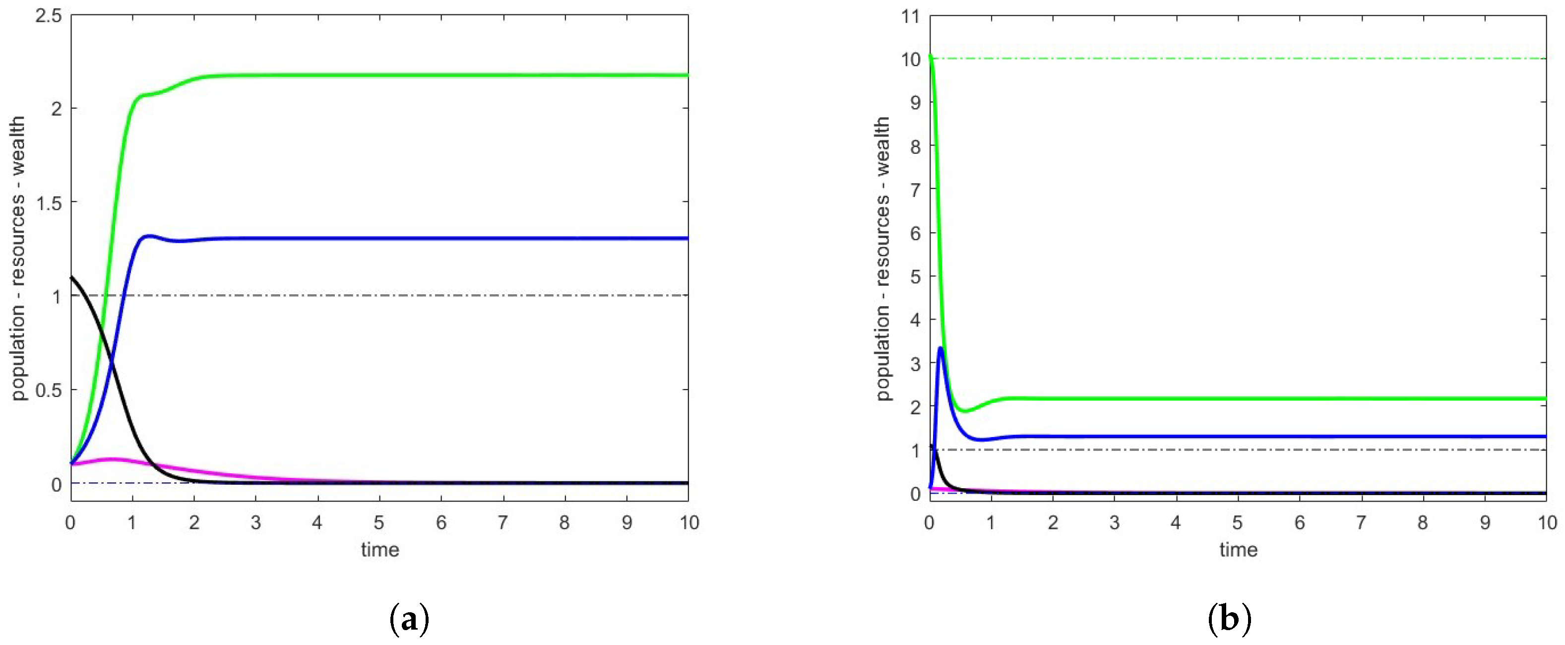
In all depicted graphs, the evolution of variables is illustrated using distinct colors: the population in magenta, renewable resources in green, non-renewable resources in black, and accumulated wealth in blue. Dashed lines indicate the coordinates of the equilibrium point under consideration, with matching colors for corresponding components (i.e., magenta for the population, and so forth).

In these simulations, we aimed to test our theoretical analyses by depicting in each chart a dashed line that represents the equilibrium point and a curve that results from uniformly perturbing the initial value relative to the equilibrium point. Alongside these verifications, we analyzed the behavior of the solution curves as the depletion coefficient $\delta$ of both renewable and non-renewable resources increases, sometimes obtaining results different from those achieved for a small $\delta$ (in the literature small $\delta$s are usually considered). We also analyzed the behavior of the solutions obtained by considering different depletion factors between renewable and non-renewable resources. Finally, we tested the stability of some equilibrium points supporting positive values for all the variables. On the x-axis, we use a generic unit of time that does not correspond to specific intervals such as days, months, or years, and does not necessarily span long periods. Indeed, we suspend our simulation once the expected behavior becomes clear. On the y-axis, the label "resources" refers to both renewable and non-renewable resources. This simplification was dictated by space constraints.

In these experiments, we kept certain parameter values constant, setting them to the values generally found in the literature (see [6,9]). However, we deliberately altered other parameters to study their behavior. In particular, if not stated otherwise in the comment of the individual figure, we consider the nature carrying capacity $\lambda =100$, the nature regeneration factor $\gamma =0.01$, the wealth consumption $\sigma =5$, the factor that regulates the possible increase of non-renewable resources $k=1$, and, finally, the factors that govern the dynamics of populations $c=1,d=3,\mu =2$. Our simulations, on the other hand, were conducted by varying the parameter $\delta$.

In analyzing the correctness of our theoretical studies, we started from the case $x\le w$, that is, when wealth is greater than the current population. When $w=0$ the critical points are given by two families of points that we have denoted by Q and R, representing the desert state and the nature state, respectively. These are two families of unstable points that in Figure 1 we have represented in the case of $\delta =3,Z=1$. To achieve better chart readability with variable values of the same order of magnitude, we set $\lambda =10,\gamma =0.5$.

We then analyzed the situation near the critical points of case (ii.2) both to verify the correctness of our analysis and to observe the potential scenarios around such points. The theoretical results obtained for small $\delta$ predict instability at point $P_1$, whereas for point $P_2$, we observe instability when $\gamma \lambda -k>0$ and stability otherwise. We have depicted in Figure 2a the scenario that emerges from a situation close to point $P_1=(0,0,9.4054,0.9387)$ with $\delta =0.49<k/2$. The eigenvalues of $J\left(P_1\right)$ are ${\rho }_k=0.0294,-4.7227,-1.0,0.5316$, indicating an unstable situation according to theory. This behavior was confirmed by various numerical simulations for both a small $\delta$ and a potentially large $\delta$ value. In Figure 2b, we present the expected situation following a perturbation of point $P_2$ when $\gamma \lambda -k=-0.9<0$ with $\lambda =10$, that is, in a situation of stability. Thus, we identify the critical point $P_2=(0,0,10.6748,1.0653)$ with eigenvalues of $J\left(P_2\right)$ as ${\rho }_k=-0.0338,-5.2929,-1.0000,-0.4316$, stable according to the theory. We also examined the behavior of $P_2$ with a large $\delta$ value. For example, in the case $\delta =5$, by setting $k=2\delta +0.5=10.5$, and thus $\gamma \lambda -k=-9.5$, we obtained $P_2=(0,0,1.3702,1.3702)$ and the following eigenvalues for $J\left(P_2\right)$: ${\rho }_k=-3.4254\pm 1.6053i,-1.0000,-5.8508$. The numerical results align with our predictions both when $\gamma \lambda -k<0$ and $\gamma \lambda -k>0$.

We have now included an example of our simulation for large values of $\delta$. This is just one among many tests we conducted without complete theoretical support. Because of this, we are eager to explore this area further in future research. In Figure 3, we present the analysis of point P in case (ii.3) for large values of $\delta$. We recall that in case (ii.3), there exists a single stable critical point when $k\lambda -\sigma <0$ and it becomes unstable if the condition is reversed. This analysis has been validated through numerous simulations with small $\delta$. It should be noted that, in the case of stability, the basin of attraction of the point is very small and the perturbation applied to P had to be minimized to ensure convergence to this equilibrium point. With the standard perturbation $ϵ={10}^{-1}$, the system tends to converge towards point $P_1$ of case (ii.7), which only differs from P in the population values. In Figure 3, we detail the analysis of point $P=(0,0.0500,0,0.1000)$ for $\delta =10$. In Figure 3a, the outcomes for $k\lambda -\sigma >0$, specifically $k\lambda -\sigma =95$, are shown. Here, P is established as a stable point, irrespective of $k\lambda -\sigma$ values. However, it is crucial to highlight that the attraction basin of this point is exceedingly narrow. Similar to the previously mentioned scenario for small $\delta$, it was necessary to reduce the standard perturbation to $ϵ={10}^{-3}$ to ensure convergence to point P instead of point $P_1=(0.1308,0.00500,0,0.01000)$ of case (ii.7), which remains stable under identical convergence conditions for $\delta \to 0^{+}$. Given that P’s components are near zero, a perturbation on the order of ${10}^{-3}$ is deemed reasonable. The eigenvalues of matrix $J\left(P\right)$ are ${\rho }_k=-0.2501\pm 0.6612i,-1.0000,-0.9896$. Figure 3b explores the scenario with $k\lambda -\sigma =-2$, achieved with $k=0.3,\lambda =10$. The eigenvalues of $J\left(P\right)$ are $-0.0250\pm 0.0661i,-1.0000,-0.0999$. Stability is observed over very long intervals. Similar to the previous cases, the stable point exhibits a notably small basin of attraction. In Figure 3b, we illustrate the scenario achieved with a perturbation $ϵ={10}^{-2}$ that leads us to convergence towards the point $P_1=(0.0131,0.00500,0,0.01000)$ of case (ii.7).

We now report some experiments conducted in the case $x>w$.

Specifically, in Figure 4, we analyze, as $\delta$ varies, the behavior of solutions starting near the equilibrium point indicated as $P_{12}$ in the scenario (iii.1), predicted to be unstable if $\gamma \lambda -k>0$. In our case, we set $\gamma =0.1$ so that $\gamma \lambda -k=9>0$.

In Figure 4a, we show the behavior near $P_{12}=(9.8673,0,376.8988,7.5380)$ obtained with $\delta =0.1$. The eigenvalues of $J\left(P_{12}\right)$ are ${\rho }_k=-0.3587\pm 0.7661i,-49.3647,9.0133$.

In Figure 4b, we present the situation near the point $P_{12}=(1.2243,0,10.7251,0.9353)$ obtained with $\delta =k\sqrt{\mu t_1}/2-0.001=0.4360$, a value of $\delta$ that we consider large, given that we intend to keep the value of $k=1$ fixed while respecting the required constraints. The eigenvalues of $J\left(P_{12}\right)$ are ${\rho }_k=-0.0631,-0.4081,-6.3956,9.4662$.

In the case of $\gamma \lambda -k<0$, for which we have stability for small values of $\delta$, we observed a situation of instability by pushing $\delta$ to the maximum value allowed while keeping $k=1$ fixed.

In Figure 5, we show two examples from our work on how solutions behave when the depletion rates, ${\delta }_1$ and ${\delta }_2$ for renewable and non-renewable resources, are different. This part of our study adds an interesting twist, showing that these different rates can change how the system behaves. We think this is a good area to explore more in future research.

Specifically, in Figure 5a, we analyzed a situation similar to the one observed in Figure 3a, for the case (ii.3) with $k\lambda -\sigma =95$ being unstable according to theoretical results for $\delta \to 0^{+}$, but exhibiting behavior that contradicts this for large $\delta$. The point P under consideration depends only on ${\delta }_1$, but it would seem that the behavior of the solutions is dictated by ${\delta }_2$. Indeed, in Figure 5a, we report the situation obtained by setting ${\delta }_1=10$, resulting in point $P=(0,0.0500,0,0.1000)$, and ${\delta }_2=0.01$. The simulation provides a scenario of unstability with eigenvalues given by ${\rho }_k=-0.2501\pm 0.6612i,-1.0000,0.0089$. We have also analyzed the situation with ${\delta }_1=0.01$, ${\delta }_2=10$ in a scenario of stability, with the eigenvalues of the Jacobian matrix in $P=(0,99.8004,0,0.1996)$ given by ${\rho }_k=-0.9980\pm 0.0446i,-1.0000,-1.9577$. Therefore, the point is stable, in accordance with the behavior observed for large values of $\delta$. The chart is not significant as it shows a rapid convergence to the indicated point and is therefore not included here.

In Figure 5b, we instead report the scenario obtained for point $P_1$ in case (iii.2), again with ${\delta }_1\ne {\delta }_2$ when $k\lambda -\sigma =95>0$. It is recalled that the theoretical analysis conducted for ${\delta }_1={\delta }_2=\delta$ predicts a situation of instability for small $\delta$. However, numerical experiments have revealed a behavior of stability for large $\delta$. Returning to ${\delta }_1\ne {\delta }_2$, even in this case, $P_1$ depends only on the value of ${\delta }_1$. In the Figure 5b we have reported the result obtained with ${\delta }_1=3$ leading to $P_1=(0.3319,0.4226,0,0.2536)$ and ${\delta }_2=0.1$. This is a situation of instability, and the eigenvalues of the Jacobian matrix are ${\rho }_k=-0.1567\pm 0.7521i,-2.0957,0.0444$. The presence of a small ${\delta }_2$ thus leads us to achieve what is predicted by the theory for $\delta \to 0^{+}$. We do not report the graph of the result obtained by inverting the values of ${\delta }_1$ and ${\delta }_2$, that is, by setting ${\delta }_1=0.1$ leading to $P_1=(2.0748,79.2516,0,1.5850)$ and ${\delta }_2=3$. In this case, we achieved a situation of stability with the eigenvalues of the Jacobian matrix given by ${\rho }_k=-0.7603\pm 0.4076i,-10.3915,-5.4577$. The graph turned out to be of little significance as the stability situation was reached quickly. We therefore conclude by saying that even in the case (iii.2), as in the case of (ii.3), it would seem that ${\delta }_2$ controls the behavior of the equilibrium point whose coordinates depend only on ${\delta }_1$.

We would have liked to further analyze the scenario presented in (ii.4), because the critical point depends on both ${\delta }_1$ and ${\delta }_2$, but studies for significantly different values of the two parameters are not possible because, as they increase, the point exits the cone.

A state of stability with a positive population is depicted in Figure 6. We have analyzed the scenario described in cases (ii.8) and (iii.3) under the predicted conditions of stability as $\delta \to 0^{+}$. In both instances, we set $\delta =0.3$. Figure 6a illustrates case ii.8) where $P_{12}=(2.3138,4.6972,24.7626,1.7676)$ is stable and falls within the cone for $\gamma \lambda -k=0.3>0$, achieved with $k=0.7$, $\lambda =10$, and $\gamma =0.1$. The eigenvalues of $J\left(P_{12}\right)$ are ${\rho }_k=-0.7454,-8.5064,-0.6207,-0.1805$. Figure 6b shows case (iii.3) with $P_{12}=(2.4700,25.8987,5.5504,1.8869)$, stable and within the cone for $\gamma \lambda -k=0.1>0$, obtained with $k=0.9$. The eigenvalues of $J\left(P_{12}\right)$ are ${\rho }_k=-12.4196,-0.4555\pm 0.6858i,-0.0239$.

8. Conclusions: Main Results and Future Steps

Let us summarize the main results obtained in this paper. In Section 2, we obtained that it cannot be $x\left(t\right)\to +\infty$ or $w\left(t\right)\to +\infty$ or $z\left(t\right)\to +\infty$ as $t\to +\infty$. This does not mean that $x,w,z$ are bounded, but that, if they exceed a critical level, they will begin to oscillate. In a real society, such oscillations of population and wealth of course are not a positive thing. Hence, our results seem to suggest that, even assuming an optimistic hypothesis on the replenishment of non-renewable resources, indefinite growth in wealth (and population) is not possible, and any attempt to achieve it may have undesirable consequences. We remark that we obtained a similar result in [2]. As the model introduced in [2] is different in many respects from the present one, these asymptotic results seem to be robust.

The analysis of equilibrium points shows a much greater variety of such equilibria than the original HANDY model. This seems to indicate that the use of non-renewable resources allows human society greater freedom to choose between possible paths. We have also shown that most equilibrium points are unstable as $\delta \to 0^{+}$. However, for some ranges of the parameters, there are asymptotically stable equilibrium points, and also some that exhibit positive values for both population and wealth. These are cases (ii8) and (iii3) in Section 3, Section 5, and Section 6 (see also Figure 6 in Section 7). This suggests a possibility for a rich, consumeristic society to avoid collapse or dangerous oscillations in population and wealth. However, this requires abandoning the idea of indefinite growth in favor of seeking a steady state for the relevant variables.

Most of these results are obtained in the hypothesis of $\delta \to 0^{+}$, which means a small rate of depletion of resources. An interesting topic for future research would be to study if these results are still valid for large $\delta$s. Some simulations (which we have not reported in this paper) seem to indicate that this is not always the case, and it would be interesting to obtain some theoretical results. Another interesting topic would be to understand if there are changes in the dynamics assuming different depletion rates for renewable and non-renewable resources. See Figure 5 of Section 7 for some simulations. An interesting direction for future research would be to change the model to take into account the major importance of the non-renewable resources in our society. This will be the argument of a forthcoming paper.

References

- Motesharrei, S.; Rivas, J.; Kalnay, E. Human and nature dynamics (HANDY): Modeling inequality and use of resource in the collapse or sustainability of societies. Ecol. Econ. 2014, 101, 90–102. [Google Scholar] [CrossRef]
- Badiale, M.; Cravero, I. A HANDY type model with non renewable resources. Nonlinear Anal. Real World Appl. 2024, 77. [Google Scholar] [CrossRef]
- Motesharrei, S.; Rivas, J.; Kalnay, E.; Asrar, G.R.; Busalacchi, A.J.; Cahalan, R.F.; Cane, M.A.; Colwell, R.R.; Feng, K.; Franklin, R.S.; et al. Modeling sustainability: Population, inequality, consumption, and bidirectional coupling of the Earth and Human Systems. Natl. Sci. Rev. 2016, 3, 470–494. [Google Scholar] [CrossRef] [PubMed]
- Akhavan, N.; Yorke, A. Population collapse in Elite-dominated societies: A differential model without differential equations. SIAM J. Appl. Dyn. Syst. 2020, 19, 1736–1757. [Google Scholar] [CrossRef]
- Grammaticos, B.; Willox, R.; Satsuma, J. Revisiting the Human and Nature Dynamics Model. Regul. Chaotic Dyn. 2020, 25, 178–198. [Google Scholar] [CrossRef]
- Tonnelier, A. Sustainability or societal collapse, dynamics and bifurcations of the handy model. SIAM J. Appl. Dyn. Syst. 2023, 22, 1877–1905. [Google Scholar] [CrossRef]
- Sendera, M. Data adaptation in handy economy-ideology model. arXiv 2019, arXiv:1904.04309. [Google Scholar]
- Al-Khawaja, T.A.K.A. Mathematical Models, Analysis and Simulations of the HANDY Model with Middle Class. Ph.D. Dissertation, Oakland University, Rochester, MI, USA, 2021. Available online: https://our.oakland.edu/handle/10323/11946 (accessed on 20 March 2024).
- Shillor, M.; Kadhim, T.A. Analysis and simulation of the HANDY model with social mobility, renewables and nonrenewables. Electron. J. Differ. Equ. 2023, 2023, 1–22. [Google Scholar] [CrossRef]
- Iannelli, M.; Pugliese, A. An Introduction to Mathematical Population Dynamics; Springer: Berlin/Heidelberg, Germany, 2014. [Google Scholar]
- Gantmacher, F.R. The Theory of Matrices 2; AMS Chelsea Publishing: New York, NY, USA, 2000. [Google Scholar]
- Ben-Romdhane, M.; Temimi, H.; Baccouch, M. An iterative finite difference method for approximating the two-branched solution of Bratu’s problem. Appl. Numer. Math. 2019, 139, 62–76. [Google Scholar] [CrossRef]
Figure 1.
Case (i). Scenario around the unstable critical points. (a) . (b) .
Figure 2.
Case (ii.2), analysis of the points and , with . (a) . (b) .
Figure 3.
Case (ii.3), analysis of the point P with . (a) . (b) .
Figure 4.
Case (iii.1) analysis of the point with . (a) . (b) .
Figure 5.
Analysis for . (a) Case (ii.3). (b) Case (iii.2).
Figure 6.
Stable critical points with positive population. (a) case (ii.8). (b) case (iii.3).
Disclaimer/Publisher’s Note: The statements, opinions and data contained in all publications are solely those of the individual author(s) and contributor(s) and not of MDPI and/or the editor(s). MDPI and/or the editor(s) disclaim responsibility for any injury to people or property resulting from any ideas, methods, instructions or products referred to in the content. |
© 2024 by the authors. Licensee MDPI, Basel, Switzerland. This article is an open access article distributed under the terms and conditions of the Creative Commons Attribution (CC BY) license (https://creativecommons.org/licenses/by/4.0/).
Share and Cite
MDPI and ACS Style
Badiale, M.; Cravero, I. A Nonlinear ODE Model for a Consumeristic Society. Mathematics 2024, 12, 1253. https://doi.org/10.3390/math12081253
AMA Style
Badiale M, Cravero I. A Nonlinear ODE Model for a Consumeristic Society. Mathematics. 2024; 12(8):1253. https://doi.org/10.3390/math12081253
Chicago/Turabian StyleBadiale, Marino, and Isabella Cravero. 2024. "A Nonlinear ODE Model for a Consumeristic Society" Mathematics 12, no. 8: 1253. https://doi.org/10.3390/math12081253
Note that from the first issue of 2016, this journal uses article numbers instead of page numbers. See further details here.