A Novel Computational Instrument Based on a Universal Mixture Density Network with a Gaussian Mixture Model as a Backbone for Predicting COVID-19 Variants’ Distributions

Abstract

Various published COVID-19 models have been used in epidemiological studies and healthcare planning to model and predict the spread of the disease and appropriately realign health measures and priorities given the resource limitations in the field of healthcare. However, a significant issue arises when these models need help identifying the distribution of the constituent variants of COVID-19 infections. The emergence of such a challenge means that, given limited healthcare resources, health planning would be ineffective and cost lives. This work presents a universal neural network (NN) computational instrument for predicting the mainstream symptomatic infection rate of COVID-19 and models of the distribution of its associated variants. The NN is based on a mixture density network (MDN) with a Gaussian mixture model (GMM) object as a backbone. Twelve use cases were used to demonstrate the validity and reliability of the proposed MDN. The use cases included COVID-19 data for Canada and Saudi Arabia, two date ranges (300 and 500 days), two input data modes, and three activation functions, each with different implementations of the batch size and epoch value. This array of scenarios provided an opportunity to investigate the impacts of epistemic uncertainty (EU) and aleatoric uncertainty (AU) on the prediction model’s fitting. The model accuracy readings were in the high nineties based on a tolerance margin of 0.0125. The primary outcome of this work indicates that this easy-to-use universal MDN helps provide reliable predictions of COVID-19 variant distributions and the corresponding synthesized profile of the mainstream infection rate.

1. Introduction

Research teams from many countries have prioritized the study of the spread of the COVID-19 virus to combat its threat to health. As a result, numerous mathematical models have been developed to study the virus’s transmission [1,2,3,4,5,6,7,8,9,10,11,12,13,14,15,16,17,18,19,20,21,22,23,24,25,26,27,28,29,30,31,32,33,34]. From a statistical perspective, these models can be classified into deterministic staging or compartmental models (CMs) [1,2,3,4,5,6,7,8,9,10,11] and stochastic models (SMs) [12,13]. In addition, machine learning (ML) [15,16,17,18,19] and neural networks (NNs) [20,21,22,23,24,25,26,27,28] have also been used to create COVID-19 models. In some cases, ML technology has been used for COVID-19 diagnosis [28,29] and prognosis [30]. However, these studies focused on models that only targeted the growth of the mainstream symptomatic infection rate of COVID-19 and have yet to address its symptomatic variants. Therefore, the gap in these mathematical modelling techniques can be addressed by briefly reviewing the CM, SM, and ML approaches. This communication identifies and addresses this technical gap, which is the impetus for creating multi-variant models of COVID-19.

CMs are models with fixed input variables, and they are considered deterministic models. Providing consistent epidemiological projections for a pandemic is one of the essential techniques for planning and deploying appropriate healthcare procedures, as well as establishing which remedies and interventions are the most effective. From the perspective of statistical models, the main challenges are uncertainties in the collected data, the inhomogeneous assembly of datasets across different local health authorities, and the limited capability for conducting tests and attaining the associated results to classify infection variants’ contributions. These same challenges are natural obstacles to using ML and NNs for the modelling and prediction of the infection rate and potential variant growth.

The complexity of a CM depends on the following formal elements:

(1)

The number of compartments or stages (M);

(2)

The forward and backward inner flows between the compartments;

(3)

The weighting parameters;

(4)

The number of numerical computation libraries.

A CM depends on the critical assumption that the total population in a given infection cycle is constant within the framework that defines that model. This postulation allows one to consider that the time derivative of the n^th compartment can be considered as the rate of individuals’ transition to the (n ± k)^th compartment, where n, k = {1, 2, …, M} and n ≠ k. This cascading form constitutes a system of ordinary differential equations (SODE). Consequently, we can build simple to complex CMs depending on the number and details of the formal elements. To find an optimal solution for an SODE, one must optimize the whole system of equations, not the individual equations [1,2]. While it is possible to find an analytical solution for a simple (i.e., M = 3 and no backward flows) CM, a system’s optimal solution can typically be found using a numerical computation library, such as the Python Differential Evolution (DE) library [35]. The optimal solution and the framework are the foundational pillars of the targeted model of the COVID-19 infection rate. Such a model can be as simple as SIR [3,4] (susceptible, infected, and recovered), as detailed as SEIR [4,5,6] (susceptible, exposed, infected, and recovered), or as extensive as those in [1,2,7,8,9] with many backward flows.

When considering variations in the input variables, one can produce a stochastic model (SM) [12,13]. One of the characteristics of the SM approach is that one can characterize the model’s output in terms of probability. Such a model allows random multi-dimensional time variations. This means that the probability distribution of the COVID-19 transition rate within an epidemic cycle can be conditioned by the possible influence of the associated health environment and noise from working procedures. Both simple and complex models can be formulated depending on the number of influencing variables and their assumed probability distributions, to compute an average over the plausible range of values. Based on the derived model, the computed set of average value predictions form an infection forecast profile over a period beyond the data range of the model itself.

Before summarizing the research efforts related to ML, it is worth mentioning that the ML survey papers presented in [31,32,33] reveal astonishing research statistics that reflect the advancements in open-source ML libraries and computing horsepower. The authors of [31] assessed 126,978 titles and 412 studies detailing 731 novel prediction models or validations thereof. Among the 731 models, 125 were diagnostic ML models (with 75 using medical imaging). At the same time, the remaining 606 were predictive models (13 models) or models that predicted different outcomes for the general population and those with confirmed cases (593 models). The studies presented in [28,29,30] are examples of diagnostic and prognostic research using ML. The report in [32] identified 920 conference presentations, review articles, algorithmic descriptions, and case studies providing organzational options related to ML and NNs. The communication in [29] characterized the published COVID-19 forecasting papers based on the algorithms used and the implementation approaches. The main algorithms can be summarized as follows: the simple moving average; auto-regressive integrated moving average (ARIMA); two-piece distributions based on the scale; logistic functions, such as S-shaped functions for modelling epidemiological curves; regression methods; canonical neural networks; deep learning methods based on convolutional neural networks (CNN); and deep learning methods based on long short-term memory (LSTM) neural networks. Implementations include genetic programming and classical/modified compartmental models: SIR, SEIR, and SEIRD. However, ML has been a critical mathematical research tool since the outbreak of the pandemic [33].

By leveraging data-driven approaches, researchers have attempted to understand the factors influencing transmission dynamics and forecast infection rates [14,15,16,17,18,19,20,21,22,23,24,25,26,27]. For the modelling and prediction of infection growth with ML, the health data related to COVID-19 must be historically deep enough to ensure consistency and reliability for a training set to support the optimization processes within an ML test engine. The two main aspects that require focus when designing an ML solution architecture are feature engineering and building the design of the actual ML model. The first focus is on the identification of the essential features that capture the complex dynamics of the pandemic’s spread. The size of the elements in the feature set should be sufficient to formulate the mapping and flow relationships of the independent input variables’ domain with the corresponding output set or sets. This detailed mapping allows the ML model to weave the fabric of the data framework within its deployed layers. Brief examples of these features of COVID-19 include the following:

(1)

regional density distribution;

(2)

age categories;

(3)

social distancing and masking;

(4)

vaccination;

(5)

climate data;

(6)

asymptomatic infection;

(7)

healthcare resources.

The second focus is on designing and building an actual ML layering model for the profile of the curve of the growth rate. This step requires (a) ML algorithms for the prediction and modelling of COVID-19, as well as (b) predictive analysis and forecasting. By training a model on published data, researchers can forecast infection rate profiles, identify potential hotspots, and estimate the effectiveness of containment measures.

The predictive modelling approaches using CMs in [2,3,4,5,6,7,8,9], using SMs in [12,13], and using ML in [15,16,17,18,19,20,21,22,23,24,25,26,27,28] share one statistical and computational characteristic, based on which the model of the infection rate I(t) is formed. This common characteristic is the average value set {$\widehat{I_j}$}, where j є {0,1, 2, …, J}, and J is the total number of compartmental observations of infections. The modelling and prediction work in [1] differed from that in [2,3,4,5,6,7,8,9,10,11,12,13,14,15,16,17,18,19,20,21,22,23,24,25,26,27,28]. The team in this study used an extended SEIR model, which they called PCom-SEIR. They implemented the Python Differential Evolution (DE) library to determine the optimal solution for the whole system of differential equations in PCom-SEIR as the average rate profile for each stage/compartment. Based on this approach, the researchers eventually produced separate rate profiles for COVID-19 variants.

Vanilla-type ML approaches are fit for modelling and predicting outputs based on a set of average values, but they need to be more capable of producing models and predictions for a set of average profiles. The latter is the required numerical computational path for modelling and predicting COVID-19 variants’ infection rates. No ML or NN studies have addressed the modelling of the distribution of multiple variants of COVID-19, nor have they addressed the contributions of individual variants. Consequently, this deficiency limits proper resource health planning, which costs lives and money. To overcome these challenges, in this work, we propose a practical and reliable computational engine using an MDN with GMM as a backbone. The design of the anticipated MDN architecture comprises one dense input layer, two hidden dense layers, an output layer set that consists of three specialized dense sublayers, and one concatenation layer. The output represents a set of predicted rate profiles of each COVID-19 symptomatic infection variant and the associated variant’s contribution. Then, the prediction of the overall symptomatic infection rate of COVID-19 is synthesized. In addition, in this study, the impact of noise in the input data (randomness) on model fitting is discussed. Furthermore, the determination and results of the model accuracy are discussed.

When implementing the design of the proposed MDN, we faced many challenges. One of the most challenging aspects of this work was assessing the failure of model fitting and changing the configuration of the network implementation accordingly. Implementing changes could involve one or more NN configuration elements (batch size, epochs, activation function, etc.). In addition, from an early stage, the design of an NN architecture should be identified to provide the flexibility to close computing gaps and eventually deliver the necessary results that furbish a solution with which one can answer the critical questions to help create the right health plans for combatting the spread of COVID-19 infection.

The sections of this article address the challenges in the work and pave the way to the delivery of an MDN supported by logical and valid results. Section 2 reveals the concept of the two input modes and exposes the steps for deriving the solution of PCom-SEIR for the mainstream COVID-19 infection rate. In addition, this section explains the reason for using two input runs. Section 3 discusses the evaluation of the design of an MDN for modelling COVID-19 variants. The audience of this study could range from NN experts to health professionals working for health authorities. Hence, we divided this section into three subsections because of the broad spectrum of the readers’ backgrounds. The first subsection presents an introductory overview of the NN technology. The second subsection introduces the theory behind the MDN. The third subsection presents notes about the architecture, design, and implementation of the MDN. Section 4 presents results covering two sets of twelve use cases—one for Canada and the other for Saudi Arabia. In this section, we present a table that maps the twenty-four sub-use cases to the corresponding diagrams to ease navigation through the reported results. These sub-use cases cover different data-range scenarios, two input data modes (to explore the influence of two kinds of uncertainty (epistemic and aleatoric uncertainty) on the model fitting and accuracy), and the implementations of three activation functions. In Section 5, we present the conclusions, the most important of which is that the proposed MDN is a valid and reliable tool for predicting the distribution of COVID-19 variants.

2. COVID-19 Input Data Modes

To deploy the MDN [36], we devised two input modes for the implementation, as shown in the diagram of the topology depicted in Figure 1. At an abstract level, the difference between the two modes was the degree of noise embedded in the data (randomness). The first mode was based on using raw data on COVID-19 from the WHO [37], which we expected to have a high noise level due to the natural data uncertainty and possible irregularities in the collection process. These two sources of data noise reduced the continuity (i.e., the potential absence of the data profile’s first and/or second derivative). The second mode involved the optimal solution of a modified PCom-SEIR SODE from [1]. The set of data that formed the optimal solution was expected to have less uncertainty due to the inherent curve smoothing, which led to continuity in the profile. Below, we show the steps of modifying the derivation to obtain only the mainstream infection rate.

The modification of the PCom-SEIR system eliminated the differential equations that represent COVID-19 variants, which are shown in Equation (5). This modification resulted in the following SODE:

$$\frac{dS\left(t\right)}{dt}=-\left(\alpha +\beta \frac{I}{N}\right)S\left(t\right)$$

(1)

$$\frac{dP\left(t\right)}{dt}=\alpha S\left(t\right)-\left({\Phi }_e+{\Phi }_m\right)P\left(t\right), \mathrm{where} \left({\mathsf{\Phi }}_e+{\mathsf{\Phi }}_m\right)=\mathsf{\Phi }$$

(2)

$$\frac{dE\left(t\right)}{dt}=\beta S\left(t\right)\frac{I}{N}-ϵ E\left(t\right)+\gamma E\left(t\right)$$

(3)

$$\frac{dM\left(t\right)}{dt}=ϵ E\left(t\right)-{\Phi }_{m}P\left(t\right)$$

(4)

$$\frac{dI\left(t\right)}{dt}=-\left(\delta +\mathsf{\eta }+\lambda \right) I\left(t\right)+\gamma E\left(t\right)+{\Phi }_{e}P\left(t\right)+rR\left(t\right)$$

(5)

$$\frac{dH\left(t\right)}{dt}=\delta I\left(t\right)-\left(\mathsf{{\rm X}}+\rho \right)H\left(t\right)+\phi Q\left(t\right)$$

(6)

$$\frac{dQ\left(t\right)}{dt}=\mathsf{\eta }I\left(\mathrm{t}\right)-\left(\mu +\mathsf{\sigma }+\phi \right) Q\left(t\right)$$

(7)

$$\frac{dD\left(t\right)}{dt}=\lambda I\left(t\right)+\rho H\left(t\right)+\mathsf{\sigma } Q\left(t\right)$$

(8)

$$\frac{dR\left(t\right)}{dt}=\mathsf{{\rm X}} H\left(t\right)+\mu Q\left(t\right)-\mathrm{r} R\left(\mathrm{t}\right)$$

(9)

The relationships in Equations (1)–(9) form the structural foundations that steer the transition dynamics within the life cycle of COVID-19, as shown in Figure 2. To ease the mapping between Equations (1)–(9) and the PCom-SEIR framework shown in Figure 2, we created two tables:

• One in which the time-dependent variable of the infection compartment’s population is Z(t), at which Z(t) $\in$ {S(t), P(t), E(t), I(t), M(t), H(t), Q(t), D(t), R(t)}.

  Table 1. Description of the time-dependent variables in the equations.

  	Variable (Z(t))	Description
  1	S(t)	The population of the susceptible compartment.
  2	P(t)	The population of the protected compartment.
  3	E(t)	The population of the exposed compartment.
  4	I(t)	The infection population of the symptomatic infection compartment.
  5	M(t)	The population with asymptomatic infection.
  6	Q(t)	The population of the quarantined compartment.
  7	H(t)	The population of the hospitalised compartment.
  8	D(t)	The population of the dead compartment.

  exhibits the definitions of the mentioned time-dependent variables. For the rest of this communication, the time-independent notation for the compartment rate variables is dropped to facilitate reading, when necessary.
• The compartment parameter variable ψ is defined as ψ $\in$ {α, β, є, ϒ, δ, η, λ, μ, χ, σ, ρ, φ}.

  Table 2. Description of the input parameters of the equations.

  	Parameter (ψ)	Input Parameter
  		From Compartment	To Compartment
  1	α	Susceptible (S)	Protected (P)
  2	Β		Exposed (E)
  3	Φ	Protected (P)
  4	Φe	Protected Pe = P * Φe component	Symptomatic infection (I)
  5	Φm	Protected Pm = P * Φm component	Asymptomatic infection (M)
  6	ϒ	Exposed (E)	Symptomatic infection (I)
  7	є		Asymptomatic infection (M)
  8	I	Symptomatic infection (I)	Symptomatic infection
  9	ϒ	Exposed component	Symptomatic infection (I)
  10	η		Quarantine (Q)
  11	λ		Death (D)
  12	Τ	Asymptomatic (M)	Recovered (R)
  13	Χ	Hospitalisation (H)	Recovered (R)
  14	Ρ		Death (D)
  15	Μ	Quarantine (Q)	Recovered (R)
  16	Σ		Death (D)
  17	Φ		Hospitalisation (H)
  18	r	Recovered component	Symptomatic infection

  exhibits the definitions of these parameters as the weights from the input compartment to the target compartment.

The use case for Canada showed the inherent influence of the combination of federal and various provincial health controls and district statistical measures. On the contrary, the use case for Saudi Arabia revealed that there was one central health system with one set of statistical measures [2].

We employed a derivative-free optimization strategy, as in an intelligent search challenge [35,38]. As a core optimization challenge, one or more computational agents were utilized to find the optima in a real-valued search space with the embedded set of initial conditions [39]. Particle swarm optimization (PSO) [40] and differential evolution (DE) [35] are two of the most outstanding procedures. DE uses a sort of differential operator that could be easily invoked and applied via the adjustment of the model parameters [39] defined in Equations (1)–(9). The optimal solutions for differential Equations (1)–(9) are shown in Figure 3 and Figure 4 for Canada and Saudi Arabia, respectively.

3. Mixture Density Network (MDN) with Multiple Outputs

This section explains the evolution of the concept of the MDN, starting from a simple neural network (NN). This review includes four subsections, allowing the reader to skip the subsections that seem elementary or familiar. This first subsection starts with a simple neural network (NN) with one average target data output and a probability density (pd) based on a parametric set of two elements. The second part provides the theory and the logical progression of the NN to a full-fledged MDN. The architecture, design, and implementation required to run the MDN code are covered in the third subsection.

3.1. Neural Networks (NNs): An Introductory Overview

An NN with one output typically consists of an input layer, one or more hidden layers, and an output layer, as depicted in Figure 5. Each layer contains neurons, nodes, or units (in this study, we will use the word “neurons”), and these neurons are interconnected with each other through weighted connections. The input value x_i of the processing unit is multiplied by the connection weight w_kj, which simulates the learning in an artificial neural network (ANN) by adjusting the strength or weight of the connection.

The relationship between the input (x) and output (y) is then formulated as

$$y_k=f\left({\sum }_{j=o}^J{w}_{kj}{x}_{kj}\right)+\mathrm{bias}$$

(10)

This relationship is a reflection of the model’s hypothesis, which is embedded in the controlled hidden layer. The function $f$, whose input is weighted and can be shifted by the bias when needed, allows the algorithm to learn the governing relationship.

A simple feedforward NN [41] consists of

(1)

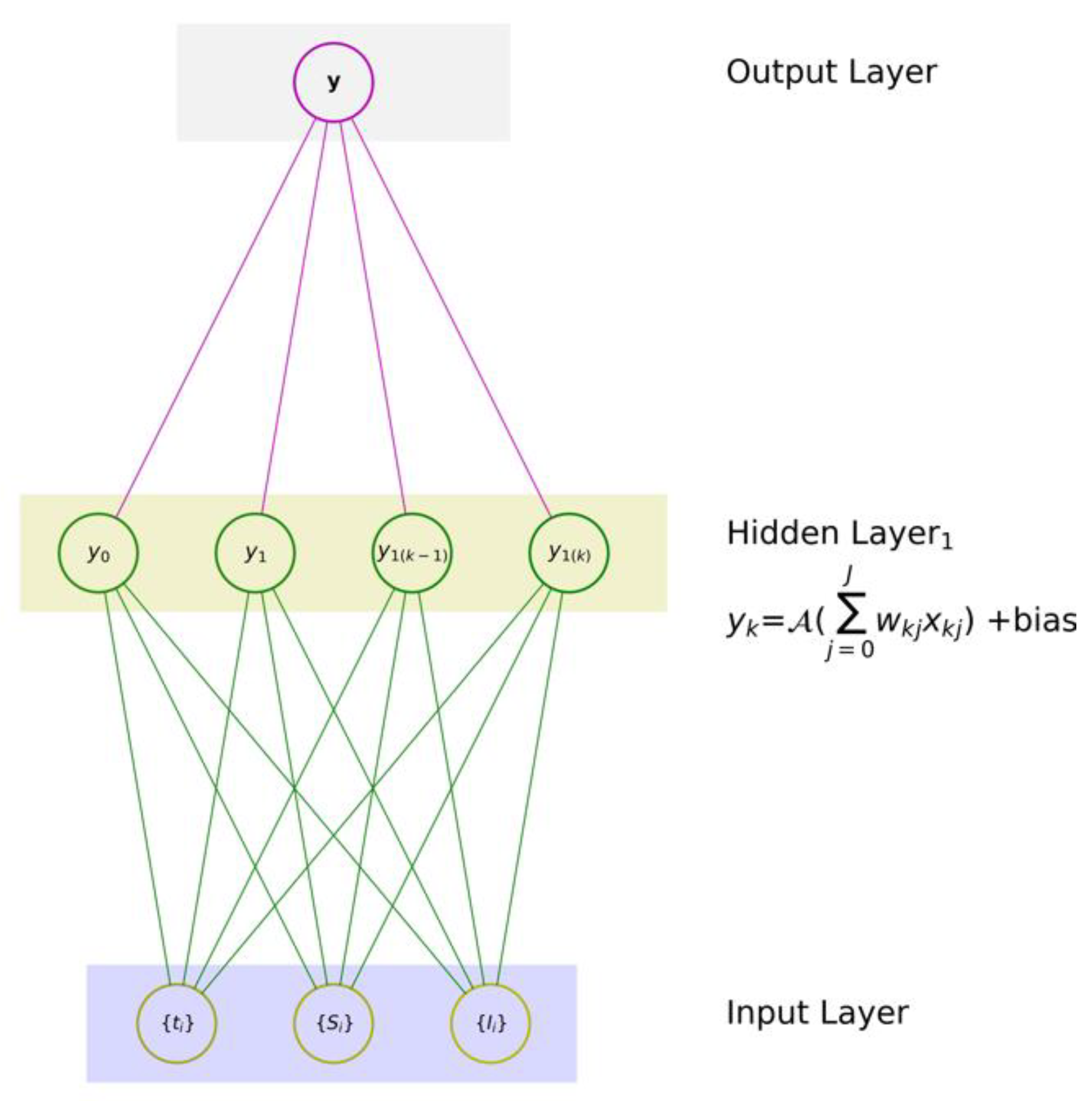
one input layer that digests a given set of input variables x ≡ {x₁, x₂, …, x_J}, where J is the number of input features,

(2)

one hidden layer with K neurons, and

(3)

one output layer with one neuron to produce an associated mapping y.

An NN model deploys an associated mapping to learn a transformation from a given set of input variables x to a set of output variables y ≡ {y₁, y₂, …, y_n}. In practice, such a network is trained to utilize a finite set of samples, which can be denoted by [{x}_q, {y}_q], where q = 1, 2, …, Q are the training sets under investigation. In other words, the principal aim of network training is to model the causal sources of event data. Hence, the best possible predictions for the y vector can be made when the trained network is presented with a new value of x. The data source can be expressed statistically in terms of the probability density function (PDF) p(x, y) in a joint-input target space.

A joint PDF with time as an additional independent variable is required if the data source evolves over time. For temporal data, in time-series analysis, the time itself (i.e., timestamps) can be a feature that is used directly in the input layer. For example, in a dataset containing recordings of daily infected populations, the date or time of the day can be an explicit input feature. However, instead of using the raw date/time values, neural networks (NNs) can learn temporal relationships implicitly. In sequential data such as published COVID-19 data, the position of a data point within the sequence (time step) can be implicitly encoded as a feature. RNNs, long short-term memory (LSTM) networks, gated recurrent units (GRUs), and other sequential models are particularly suitable for handling time-related data (e.g., windowing/time windows (TWs) and temporal embeddings (TEs)), due to their ability to maintain memory across time steps.

In summary, time can indeed be treated as an input feature in neural networks, especially when dealing with sequential or time-dependent data such as collected COVID-19 data [37], and it can be represented in various ways depending on the problem domain and data characteristics. While RNNs, LSTM networks, and GRUs are valid approaches, they have their underlying problems. The reason for this is that TWs and TEs might suppress important behaviors that exist in x, leading to an inaccurate prediction of y. Nevertheless, these techniques are good for comparing and assessing the validity of a proposed NN design. For associated mapping scenarios, such as that of the COVID-19 infection rate that we consider in this study, it is suitable to decompose the joint probability density p(x, y) into the product of the conditional density of the target data p(y|x), which is conditioned on that of the input data p(x) [41]: p(x,y) = p(y|x) p(x), where the density p(x) = ∫ p(x,y) dy plays a crucial role in confirming the predictions of the trained networks. Nevertheless, to predict the value of y corresponding to the input set {x_j} of feature x, we need to focus on the conditional density p(y|x) model rather than the average target value. This is a fundamental aspect on which we should keep our focus.

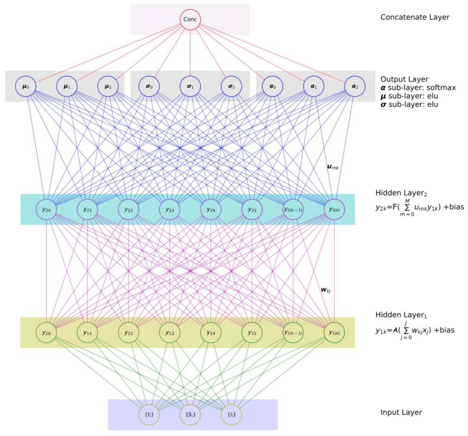
3.2. Mixture Density Network (MDN): The Theory

Typically, data scientists apply GMMs with regression and classification techniques to build the targeted MDN, and the architecture provides the necessary solution for the underlying statistical problem. However, it is known that GMMs perform clustering far better than well-known techniques such as K-means [42]. A GMM, as a computational entity within an MDN, produces a set of COVID-19 variants/subsamples {I_n(t)}, where n є {1, 2, …, N}, and N is the maximum number of variants in a COVID-19 infection wave. The GMM is computationally equipped to determine the {I_n(t)} set from the corresponding infected population I(t), which is a principal input into the input layer (Figure 1).

I(t) can be logically assumed to be normally distributed, even if it does not fall under the case of a normal distribution. This is possible because any random variable can be transformed from its actual distribution into a normal distribution [43]. Nevertheless, one might be able to find two or more variants (subsamples) of data for I(t) that can indeed be described with a normal distribution. Thus, to describe the entire population of I(t), we do not assume a Gaussian distribution across the whole population but, rather, synthesize the actual underlying distribution as a mixture of Gaussian ones with different contributions (α), variances (σ), and means (µ).

A data scientist working for a health authority might be able to predict I(t) over time in the future. However, suppose that a region has a specific COVID-19 variant that dominates over another variant or other variants. In that case, it is logical to assume that there will be a definitive number of clusters/groups N of COVID-19 variants {I_n(t)}. With different health controls across regions and the nature of the variants, type j of the variant may dominate the other types k, where j, k є {1, 2, 3, …, N} and k $\ne j$. Suppose that we construct an ML regression model (e.g., an NN) to estimate the population of an individual I_n(t). In that case, we have two potential deficiencies:

(1) We can only predict the conditional µ of the distribution. This means that we will not have a definitive and complete view of the extent of I_n(t) to propose the right health control actions.

(2) The health authority will not be able to properly discriminate between the multi-modal distributions if the entire population of I(t) is characterized by a single distribution that could be assumed to be Gaussian. To overcome these two weaknesses, a simple feedforward NN for regression purposes probably looks something like that in Figure 6, where there are two output sets of the mean (µ) and variance (σ), which represent the two basic elements of the targeted distributions.

The standard NN architecture, which is shown in Figure 6, involves injecting a collection of input variables {x_q} into the input layer of the network, determining weights in a subsequent layer, and eventually modelling an estimate of the output y. Then, once a possible backpropagation action has been commenced, the weights in the NN can be altered when necessary, and the best estimate of y is eventually provided as a prediction that yields a single value. This single value is inadequate for effective health planning because different types of variants require different diagnoses, treatments, and levels of health control measures.

To overcome this challenge, we must generate an output for the probability distributions across an array of values described by sets of the mean (µ) and variance (σ), thus defining a conditional probability distribution (CPD); hence, the network must produce two outputs, not one, as depicted in Figure 6. However, in principle, the computational learning process in Figure 5 stays the same as that in Figure 6, with each forward and backward phase slightly modifying the weights (w_jk, u_jk) until the minimum error is small enough to meet the target requirements of the necessary output. In summary, the distinguishing difference is that the NN in Figure 6 produces two values: one for μ and one for σ. These two founding attributes are basically what is required to, for example, determine the PDF of the Gaussian distribution here. Consequently, to predict µ and the associated σ of the expected Gaussian distribution, there should be two neurons in the last layer (as shown in Figure 6) as opposed to one, as shown in Figure 5.

It is worth mentioning that a CNN is an implementation of an NN in which the minimization of the sum-of-squares error gives rise to network functions that approximate the conditional mean/average of the target output. When a classification in which the target variables have one of N data boundaries is required, these conditional averages denote the posterior probabilities of class membership and, thus, can be considered as providing an optimal output. Hence, for problems involving the prediction of continuous variables, the conditional average demonstrates an extremely limited portrayal of the statistical profile of the target data and will be entirely insufficient for many scenarios. The MDN is expected to overcome these limitations and provide a completely general framework for modelling conditional PDFs. The fundamental MDN form combines a CNN with a mixture density model.

We should design and build an NN that can determine more than a single distribution, to improve the above logical approach. To make this possible, we add N of {μ_n, σ_n} sets, each corresponding to one COVID-19 variant I_n(t). These distributions should be nearly sufficient to describe the known information and published data I(t) on COVID-19. It is a known fact that COVID-19 variants have different levels of population dominance. In other words, the forecasted distributions of the variants will have different levels of contribution/weight (α_n) for the synthesized I(t). To map this requirement to our new NN design, the NN output should include N of {μ_n, σ_n, α_n} sets, with each set corresponding to one predicted COVID-19 variant. The new NN design can be expected to have the layout shown in Figure 7. This MDN with a GMM as a backbone can be used to predict the individual components I_n(t) of the COVID-19 infection compartments. In conclusion, MDNs are built from two components—an NN and a mixture model [40], which is implemented in the form of a GMM object, as illustrated in Figure 8b. Hence, the output layer of an MDN should be equipped with a GMM to synthesize the hidden layer’s outputs to the relevant distribution components, as shown in Figure 7.

3.3. Architecture, Design, and Implementation Notes

The realization of Figure 7 was achieved by adopting the layering system architecture shown in Figure 8a and the implementation of the class diagram shown in Figure 8b. In Figure 8b, it can be seen that the implementation depended on the version of TensorFlow. We started with TensorFlow version 1.8.0 and then used version 2.13.0 on different machine images. This allowed us to detect any possible bugs in the versions and compare the obtained results.

4. Results and Discussion

One of the main objectives of this study was to demonstrate the ability of the MDN to provide the distribution profiles of COVID-19 variants corresponding to a set of continuous prediction models.

A comparison with the results of similar studies is an essential part of the discussion in a typical examination of new results. However, this was not possible due to the absence of such identical work. Nevertheless, the results of the variants’ distribution profiles in this study were compared with the distributions of infection variants reported in [1] with PCom-SEIR, which were based on the optimal solutions of a SODE.

4.1. Use Case Implementation Dictionary

To ease the navigation through the use cases, we created

Table 3. MDN parameters.

	MDN–GMM Network Data
	300 Data Range	500 Data Range	300 Data Range	500 Data Range
Input Data Size	319	571	283	535
Training Data Size	212	380	188	356
Testing Data Size	107	191	95	179
Output Data Size	107	191	95	179
Neurons	10	10	10	10
Batch Size	64	64	64	64
	(A) Canada		(B) Saudi Arabia

and

Table 4. The dictionary of use cases vs. implementation results.

Country	Canada						Saudi Arabia
Data Range	300–500 Days						300–500 Days
Data Input Mode	PCom-SEIR			WHO Data			PCom-SEIR			WHO Data
Activation Function	relu	tanh	sigmoid	relu	tanh	sigmoid	relu	tanh	sigmoid	relu	tanh	sigmoid
Variant’s Distribution	Figure 9A	Figure 9A	Figure 9A	Figure 11A	Figure 11A	Figure 11A	Figure 10A	Figure 10A	Figure 10A	Figure 12A	Figure 12A	Figure 12A
Loss Performance	Figure 9B(a)	Figure 9B(b)	Figure 9B(c)	Figure 11B(a)	Figure 11B(b)	Figure 11B(c)	Figure 10B(a)	Figure 10B(b)	Figure 10B(c)	Figure 12B(a)	Figure 12B(b)	Figure 12B(c)
Network Parameters	Table 3A						Table 3B

to show the mapping of these use cases and the corresponding results. The coverage of these results was based on two main groups; each leading group corresponded to the COVID-19 data from each country (Canada (Figures 9 and 11) and Saudi Arabia (Figures 10 and 12)). Each leading country group included two input mode sub-groups. Each input mode sub-group covered two data ranges. Each data range sub-group included three activation functions. Each activation function implementation utilized two epoch values {10, 20}. Consequently, there were eight scenarios for each COVID-19 variant distribution I_n(t) per country. This array of outputs should be enough to conclude the reliability and validity of the proposed MDN computational instrument. The results are divided into two categories: (1) each set of three I_n(t) values and the corresponding synthesized and predicted COVID-19 infection rate I(t) and (2) the MDN loss performance curves.

Table 4 shows the following execution parameters:

(1)

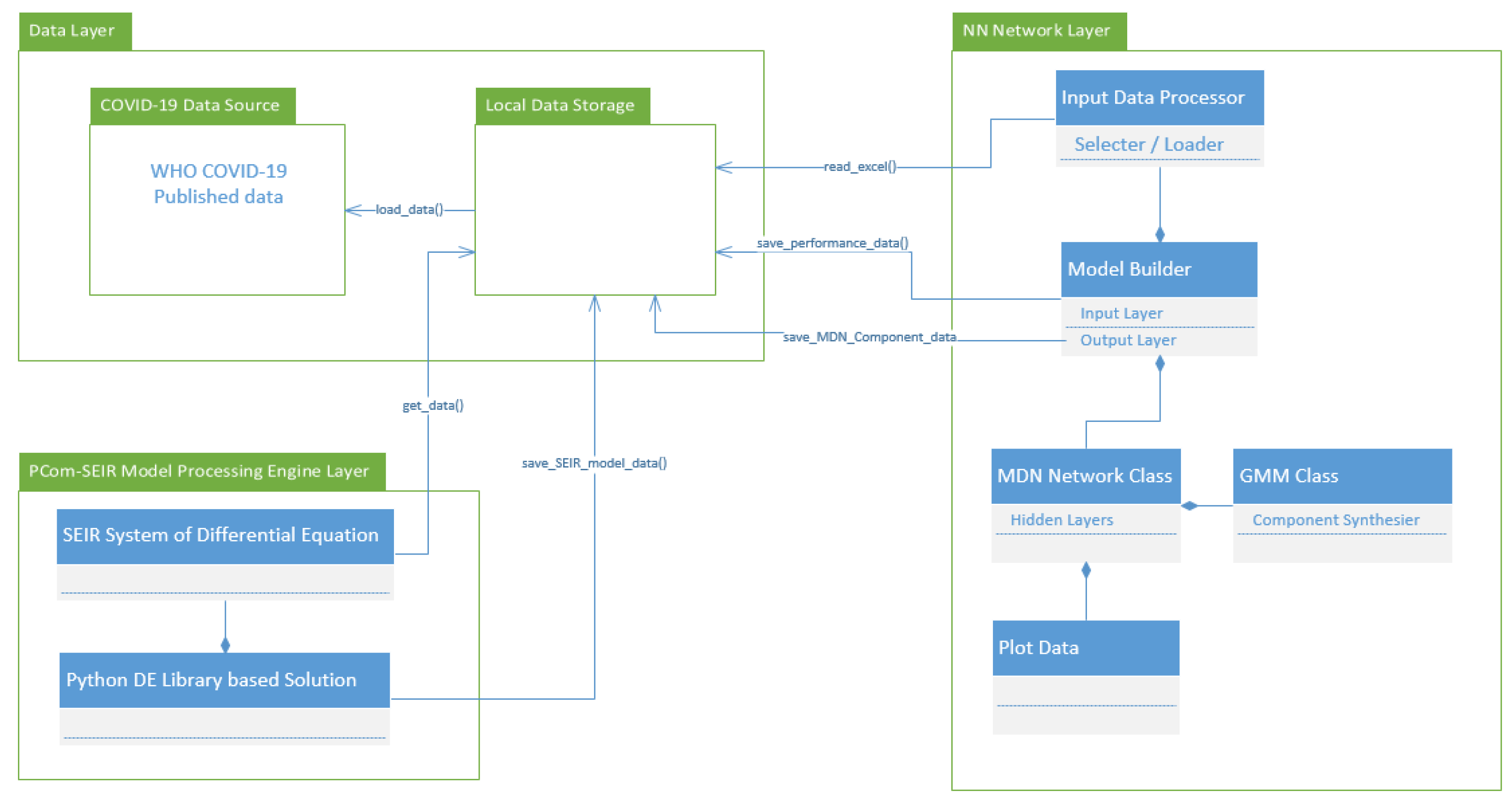
Input Modes: In Figure 1, the diagram shows the deployment of the two implementations depending on the type of COVID-19 input data for Canada and Saudi Arabia. The first input feed was raw COVID-19 data from the WHO [37]; hence, we named this source “WHO COVID-19 data”. The second input feed was the optimal solution of the SODE in Equations (1)–(9), which was derived in Section 2. The results are depicted in Figure 4 (for Canada) and Figure 5 (for Saudi Arabia). In this study, we named this input feed “PCom-SEIR” because it relied on a modification of the PCom-SEIR model.

(2)

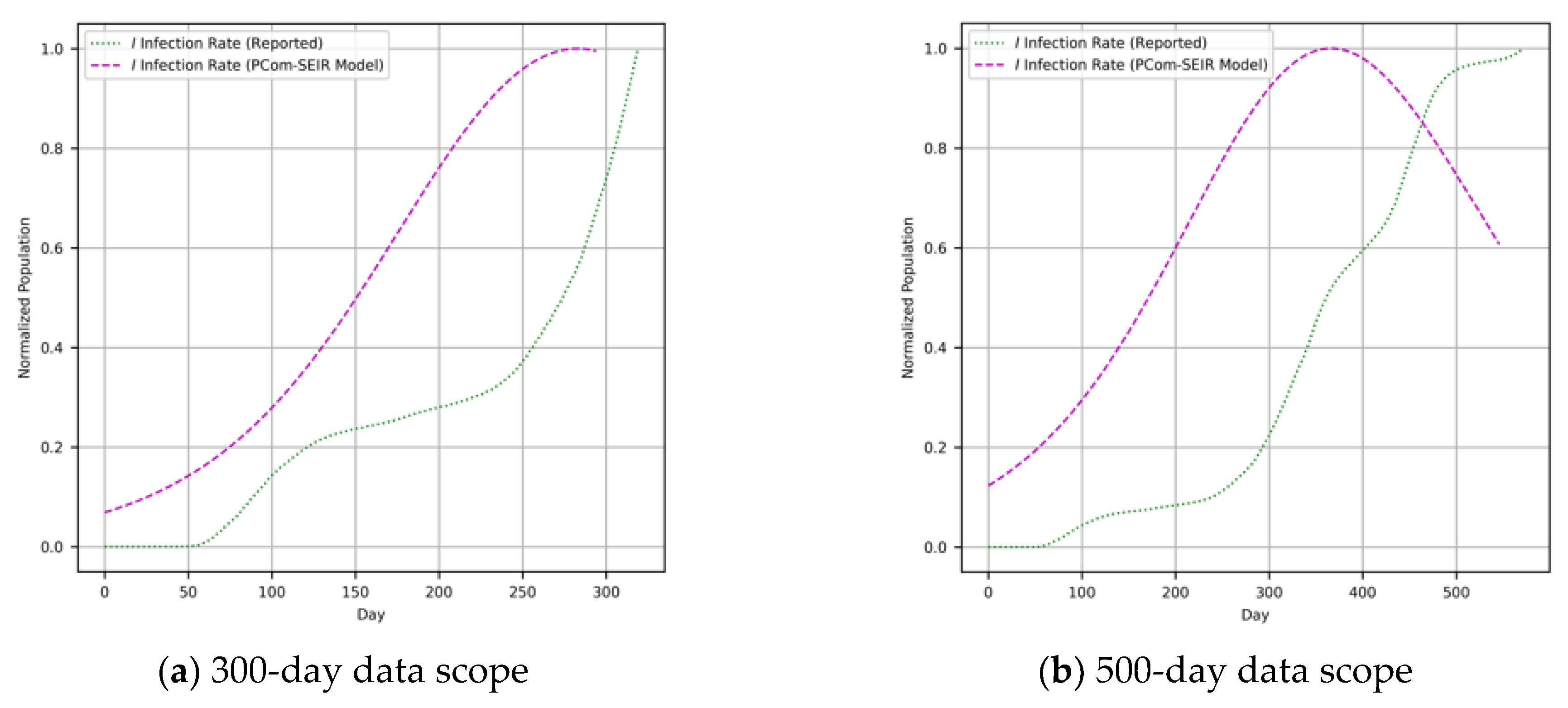
Data Ranges: The two input feeds covered two spans: 300 and 500 days.

(3)

The MDN implementation runs: There were three implementation runs; each run involved the utilization of one activation function in the hidden layers. The activation function set was {relu, tanh, sigmoid}.

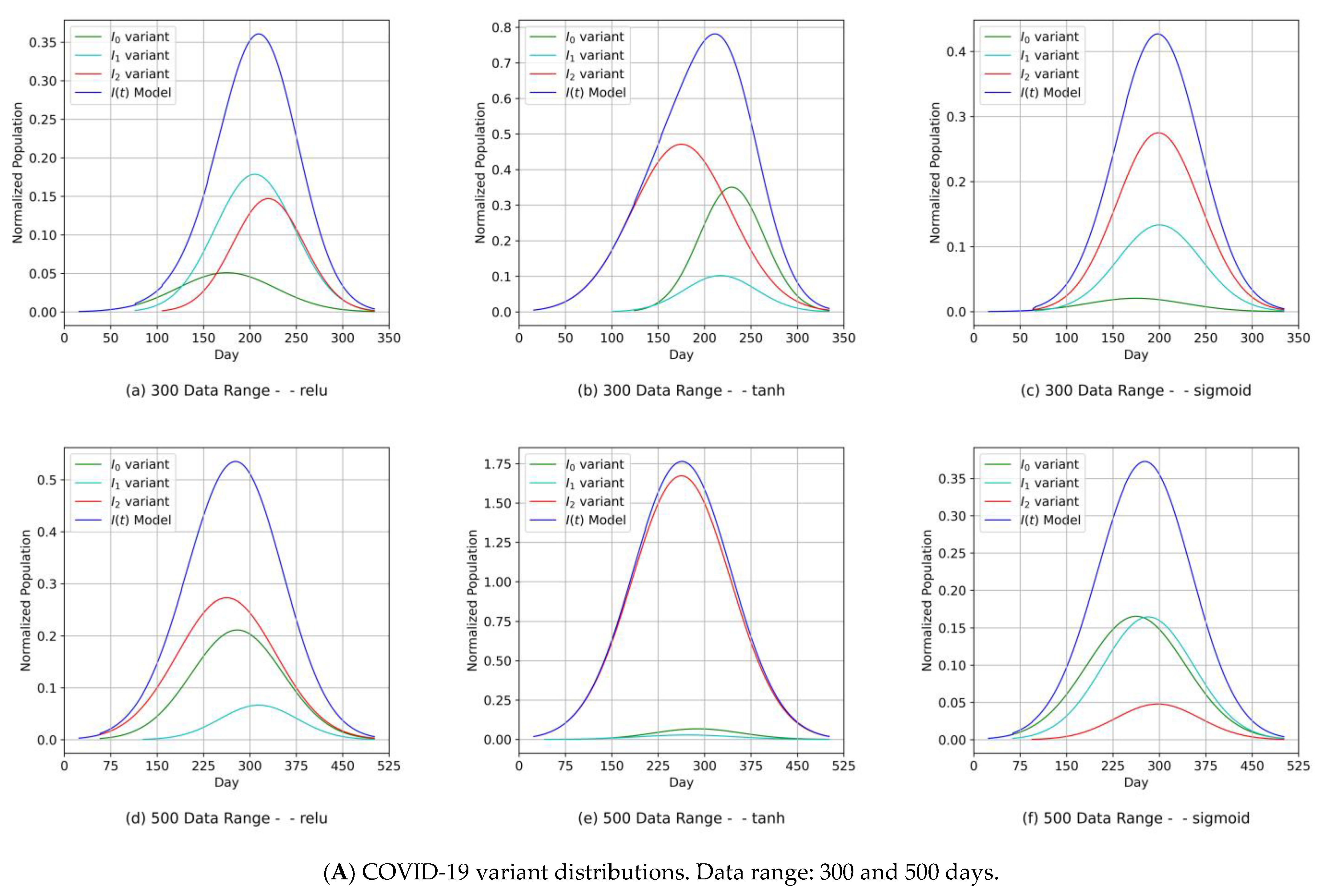
Table 4 presents the following results:

(1)

Diagrams of the COVID-19 variants’ distributions {I_n(t)} and their predicted I(t) values as a synthesized Gaussian distribution;

(2)

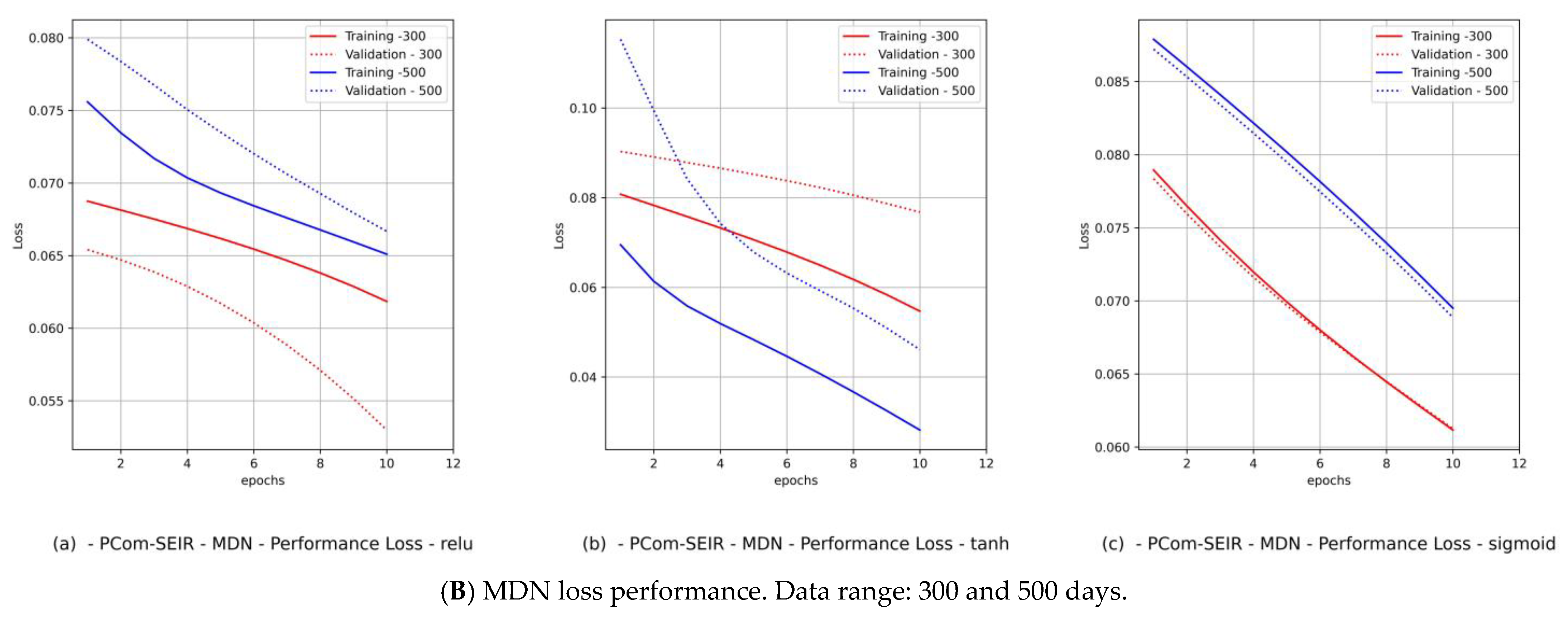
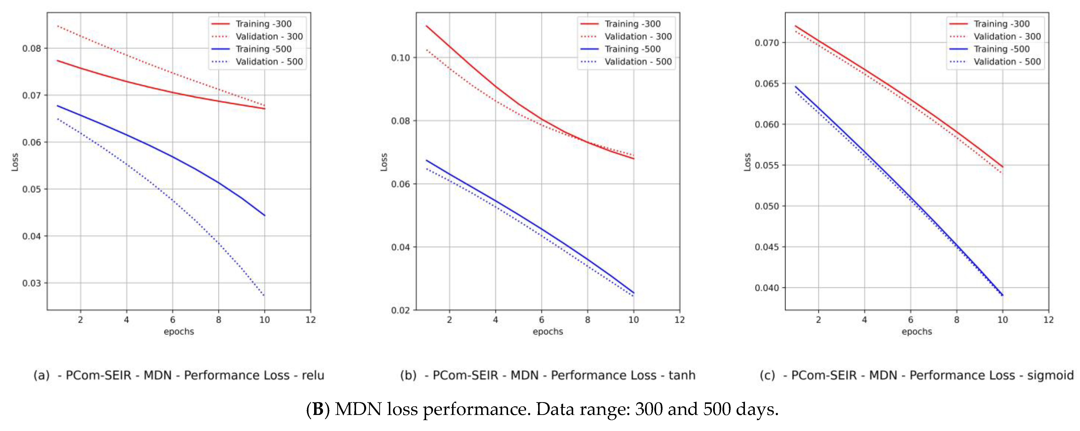
Diagrams of the MDN’s loss performance, which includes

(a)

loss vs. epochs;

(b)

val_loss vs. epochs.

4.2. Implementation Configurations and Environments

Furthermore, to show the validity and credibility of the new MDN-based computational instrument, we examined several use cases covering different input modes for COVID-19 data, date ranges, and network implementations.

The change in the implementation functionality meant that we examined the results by changing part of the implementation of the MDN design objects shown in Figure 8b and not the MDN architecture displayed in Figure 8a. While keeping the layer sequencing the same as in Figure 7, the implementation changes were fulfilled by changing the activation function in the hidden layer, which provided the average predicted distribution profiles.

We also changed the number of hidden layers, number of neurons, batch size, and number of epochs. These changes are tools for preventing overfitting/underfitting and achieving higher accuracy in modelling. Table 3 shows the main attributes of the configuration of the MDN and its practical and universal configuration when run across all use cases.

4.3. The MDN’s Predictions of COVID-19 Variants

As stated above, the input data covered two modes: (1) raw COVID-19 data, which we refer to as WHO data [37], and (2) the PCom-SEIR data, which represents the overall infection rate prediction that was computed based on the optimal solution of Equations (1)–(9). The two input datasets from Canada and Saudi Arabia, respectively, are illustrated in Figure 3 and Figure 4. These two input feeds were part of the deployment of the implementation modes depicted in Figure 1.

The proposed MDN had a layered structure, as shown in Figure 7. The network’s implementation used objects derived from the class diagram in Figure 8b. By portioning the uploaded COVID-19 data, we obtained a training set (2/3) and a test set (1/3), as shown in Table 3. A sequential model object digested the training set, while the MDN’s hidden layers processed the output from the input layer (architecture in Figure 7 and design in Figure 8b) consisting of three dense sub-layers, with each handling one of the corresponding elements of the COVID-19 variant distribution parameter set {μ_n, σ_n, α_n}. The outputs from these dense sub-layers were passed to a dense concatenation layer, which coordinated with the GMM object (Figure 7 and Figure 8b) to compute the individual COVID-19 variant profiles. In this manner, the objective of the MDN of predicting three Gaussian components, with each component corresponding to a COVID-19 variant, was fulfilled. The results are shown in Figures 9 and 11 for Canada and in Figures 10 and 12 for Saudi Arabia.

The component distribution curves, which are shown in Figure 9A, Figure 10A, Figure 11A and Figure 12A, indicate that the MDN managed to produce COVID-19 variant I_n(t) values as Gaussian distributions with different sets of distribution parameters {µ, σ, α}. As illustrated in these figures, different values of µ and σ imply that each variant candidate in the set {I_n(t)} has a different extent of time (lengths in days) and different start/end days, with the different variants’ peaks mostly taking place on different days (the unit of time of observation). Such information is vital to health authorities when planning health control measures and preparing for the impact of the spread of severe infections. The profiles of the components predicted by the MDN corresponding to COVID-19 variant I_n(t) values are different from those reported in Figure 2 and Figure 3 of [1]. In the referred study, the COVID-19 variant profiles are not fully Gaussian in shape; all variants practically share the same start and end dates but have different peaks.

4.4. The Impacts of Epistemic Uncertainty and Aleatoric Uncertainty on Component Predictions

The following discussion exposes the motives behind using two different input modes; i.e., the two types of input data shown in Figure 3 and Figure 4. From the uncertainty angle (randomness of input data), a typical supervised machine learning problem can be formulated as follows [44]:

Y = L (I, θ)

(11)

L is the learned function that maps the input I to the output Y using the parameter θ. Here, the epistemic uncertainty (EU), which describes what the model does not know, is derived from θ and the inherent aleatoric uncertainty (AU), which is part of the data-generating process of I. A high EU was found in part of the input feature space of the COVID-19 data published in [37], sporadically populated with data samples. In such an m-dimensional space, many parameters might explain the given data points, which gives rise to uncertainty. Based on this line of thinking, we decided to deploy two executions (see Figure 1) corresponding to the two data mode use cases. The first run took the output of the PCom-SEIR engine as an input (Figure 9 for Canada and Figure 10 for Saudi Arabia).

In contrast, the second run took the raw COVID-19 data from the WHO [37] (Figure 11 for Canada and Figure 12 for Saudi Arabia). The PCom-SEIR run was expected to have a lower level of EU. Regarding the AU, in a run with a larger data scope (500+ days), we could expect a higher value. In summary, we used the training loss (loss) and validation loss (val_loss) performance as footprints of the severity of the EU and AU, respectively. It is good to remember that the loss and val_loss curves reflect the level of continuity of the data and the type of deployment of the network’s constituent layers. The network layer deployment included the type of layer, the type of activation function, the batch size, and the number of epochs.

Hence, we produced loss performance curves for a set of activation functions {relu, tanh, sigmoid}. These curves are shown in Figure 9B and Figure 11B for Canada and in Figure 10B and Figure 12B for Saudi Arabia. In most deep learning projects, the graph of the loss and val_loss is a cross-validation (CV) because it encompasses the training and test data domains. The best cumulative yardstick describing the loss performance is the model fitness set {underfitting, overfitting, optimal fit} [45]. Suppose that the network input data feed has a high noise level (random fluctuations are a source of uncertainty), as in the WHO data. In that case, we would expect to have underfitting and overfitting most often. Such a scenario requires a particular activation function, batch size, and number of epochs. Similarly, if the network data feed has less noise (behavior of polarization), as in the PCom-SEIR data feed, we should expect optimal fitting more than underfitting and overfitting. The resulting mapping in

Table 5. Summary of the MDN’s loss performance.

Country		Canada				Saudi Arabia
Input Mode		PCom-SEIR		WHO		PCom-SEIR		WHO
Data Range		300	500	300	500	300	500	300	500
relu	loss
	Accuracy	97.49	98.25	97.49	76.88	96.47	98.50	96.11	99.07
tanh	loss
	Accuracy	97.49	99.30	97.81	77.93	97.88	98.88	98.23	98.88
sigmoid	loss
	Accuracy	97.18	99.12	96.87	77.76	96.11	98.13	97.17	99.44
Fitting Level %		100%	100%	33%	33%	100%	100%	33%	66%
Loss Legend		Optimal fit		Underfitting		Overfitting

shows a summary of the MDN’s loss performance, which indicates the fitting levels for the data feed and various activation functions as follows:

(1)

The fitting level of the PCom-SEIR data feed for both data ranges and both countries was 100% optimal, regardless of the activation function.

(2)

The fitting level of the WHO data for both data ranges and both countries was between 33% and 66%. The 33% optimal fitting occurred when we used the sigmoid activation function.

(3)

By observing the performance in Figure 9B(c) and Figure 11B(c) for Canada and in Figure 10B(c) and Figure 12B(c) for Saudi Arabia, one can notice that the sigmoid activation function produced 100% optimal fitting for both input data feeds. Relu and Tanh had a 100% optimal fit for the PCom-SEIR input data feed and nearly zero for the WHO input data feed. This meant that the algorithm, alongside the statistical profile of the input data, played a part in governing the model fitting for the same set of batch sizes and epochs.

4.5. The MDN Model’s Accuracy

Statistical models with complexity are referred to as flexible models. On the other hand, there are simple models that are, to a certain extent, less complex and inflexible [45] and less accurate but more interpretable. Interpretability refers to the degree to which a model allows for human understanding of natural phenomena [45]. Additionally, model flexibility indicates a model’s capacity to adapt, evolve, and learn from input data. Consequently, flexible models should be used when research aims to predict average values. However, when the objective of an investigation is inference, inflexible models are more relevant because they more easily interpret the relationship between the response variables and the predictor variables in the average profile [45]. The model in this work is a type of inflexible model.

The architecture of the proposed MDN-based computational instrument is depicted in Figure 7, and Section 2 describes the two input data (y_true) modes. The design of the architecture shown in Figure 8b suggests that there were two reference outputs. The first was a transitional output (y_tran) from the hidden layers, which fed the GMM object through the output layers. The second output was the prediction of the synthesized COVID-19 infection rate (y_pred) at the concatenation layer based on the injected output from the GMM object. Since we did not work with classification but with profile prediction using an inflexible model, we needed to define an approach for computing the model’s accuracy. A formula that equates y_pred to y_true at any observation point is defined as follows:

y_pred ± m*y_true = y_true

(12)

where m is the tolerance margin, the − sign is used when y_pred > y_true, and the + sign is used when y_pred < y_true. In our accuracy computation, we used m = 0.0125. The results are shown in Table 5. The accuracy results did not show any functional supremacy for any activation function. This observation was unexpected.

There might be a question of why we have yet to use y_tran to compute the accuracy, because y_tran is a payload of programming data between the MDN model and the GMM. Thus, in reality, y_tran is not a final prediction output. However, we tried using the accuracy_object = tf.keras.metrics.Accuracy object; then, we used accuracy_object to call update_state, which built the result dictionary object. From its numpy(), we finally obtained the accuracy reading. The accuracy reading was very low—between 5% and 55%—indicating that y_tran was not the final prediction output.

4.6. General Remarks

The error performance was extracted from the model history object (see Figure 8b), which was a dictionary object for the loss and val_loss property keys. From the loss performance diagrams in Figure 9B(a,b) and Figure 11B(a,b) and in Figure 10B(a,b) and Figure 12B(a,b) for Canada and Saudi Arabia, respectively, we can conclude that the sigmoid function showed the best performance, followed by the relu activation function.

In Figure 7, we did not include the flattening layer for our sequential COVID-19 data scenarios. In principle, this was unnecessary because flattening the data could cause a loss of sequential information in the computation of sequential data. However, we experimented with it and noticed that the loss performance (loss and val_loss) worsened tenfold.

A question might arise regarding how this new MDN can predict multiple growth peaks in the COVID-19 infection rate. Therefore, we decided to inject a hypothetical stream of COVID-19 data, as shown in Figure 13A. Surprisingly, the MDN with the sigmoid activation function produced the multipeaked I(t) shown in Figure 13B by producing one of the components as a late-peaking variant component.

5. Conclusions

The following interrelated conclusions were drawn from this research work.

(1)

The new MDN-based computational instrument was proven to be valid and credible through the examination of twelve use cases covering COVID-19 data sources, date ranges (i.e., data scope), and several MDN implementation configurations. The MDN’s outputs for these use cases clearly indicated that it produced an interpretable model for the growth of the COVID-19 infection rate [45].

(2)

Our approach can provide vital information to health authorities when planning health control measures and preparing for a severe spread of infections. This can be argued because our results indicated that the MDN produced COVID-19 variants’ In(t) values as Gaussian distributions with different sets of distribution parameters {µ, σ, α}. Different values of µ and σ imply that each variant candidate in the {In(t)} set has a different extent of time (length of days), different start/end days, and different variant peaks mostly taking place on different days (which is the unit of time of observation). Accordingly, the information above is vital to health authorities when planning health control measures and preparing for the impact of the severe spread of infections. On the other hand, in [1], the COVID-19 variant profiles had the same extent of time and practically the same peaks, as evidenced when comparing the prediction results for the COVID-19 variants’ In(t) values in this study.

(3)

Another indicator of the universality and practicality of our proposed MDN as a tool for predicting COVID-19 variants was demonstrated. It was shown that the relu, tanh, and sigmoid activation functions essentially had comparable sets of COVID-19 variant distributions, each with different parameter sets {µ, σ, α} that were compatible with the reality of the emergence and spread of COVID-19 variants.

(4)

The sigmoid function showed the best model-fitting performance, which was concluded based on the loss performance (Figure 9B, Figure 10B, Figure 11B and Figure 12B) diagrams for Canada and Saudi Arabia, as shown in Table 5.

(5)

The MDN with the sigmoid activation function produced a multipeaked I(t) value by producing one of the components as a late-peaking variant component (Figure 13).

References

1. Al-Hadeethi, Y.; El Ramley, I.F.; Mohammed, H.; Barasheed, A.Z. A New Polymorphic Comprehensive Model for COVID-19 Transition Cycle Dynamics with Extended Feed Streams to Symptomatic and Asymptomatic Infections. Mathematics 2023, 11, 1119. [Google Scholar] [CrossRef]
2. Al-Hadeethi, Y.; Ramley, I.F.E.; Sayyed, M.I. Convolution model for COVID-19 rate predictions and health effort levels computation for Saudi Arabia, France, and Canada. Sci. Rep. 2021, 11, 22664. [Google Scholar] [CrossRef] [PubMed]
3. Anastassopoulou, C.; Russo, L.; Tsakris, A.; Siettos, C. Data-based analysis, modelling and forecasting of the COVID-19 outbreak. PLoS ONE 2020, 15, e0230405. [Google Scholar] [CrossRef] [PubMed]
4. Bakhta, A.; Boiveau, T.; Maday, Y.; Mula, O. Epidemiological forecasting with model reduction of compartmental models. Application to the COVID-19 pandemic. Biology 2020, 10, 22. [Google Scholar] [CrossRef]
5. Chang, Y.-C.; Liu, C.-T. A Stochastic Multi-Strain SIR Model with Two-Dose Vaccination Rate. Mathematics 2022, 10, 1804. [Google Scholar] [CrossRef]
6. Liu, X.; Ding, Y. Stability and numerical simulations of a new SVIR model with two delays on COVID-19 booster vaccination. Mathematics 2022, 10, 1772. [Google Scholar] [CrossRef]
7. Putra, S.; Mutamar, Z.K. Estimation of parameters in the SIR epidemic model using particle swarm optimisation. Am. J. Math. Comput. Model. 2019, 4, 83–93. [Google Scholar] [CrossRef]
8. Margenov, S.; Popivanov, N.; Ugrinova, I.; Hristov, T. Mathematical Modeling and Short-Term Forecasting of the COVID-19 Epidemic in Bulgaria: SEIRS Model with Vaccination. Mathematics 2022, 10, 2570. [Google Scholar] [CrossRef]
9. Mamis, K.; Farazmand, M. Stochastic compartmental models of the COVID-19 pandemic must have temporally correlated uncertainties. Proc. R. Soc. A 2023, 479, 20220568. [Google Scholar] [CrossRef]
10. Mbuvha, R.; Marwala, T. On data-driven management of the COVID-19 outbreak in South Africa. medRxiv 2020. [Google Scholar] [CrossRef]
11. Gatto, A.; Accarino, G.; Aloisi, V.; Immorlano, F.; Donato, F.; Aloisio, G. Limits of Compartmental Models and New Opportunities for Machine Learning: A Case Study to Forecast the Second Wave of COVID-19 Hospitalizations in Lombardy, Italy. Informatics 2021, 8, 57. [Google Scholar] [CrossRef]
12. Wondyfraw, T.A.; Sama, S.T. Stochastic model of the transmission dynamics of COVID-19 pandemic. Adv. Differ. Equ. 2021, 2021, 457. [Google Scholar]
13. Hoertel, N.; Blachier, M.; Blanco, C.; Olfson, M.; Massetti, M.; Rico, M.S.; Limosin, F.; Leleu, H. A stochastic agent-based model of the SARS-CoV-2 epidemic in France. Nat. Med. 2020, 26, 1417–1421. [Google Scholar] [CrossRef] [PubMed]
14. Yan, L.; Zhang, H.T.; Xiao, Y.; Wang, M.; Guo, Y.; Sun, C.; Tang, X.; Jing, L.; Li, S.; Zhang, M.; et al. Prediction of criticality in patients with severe COVID-19 infection using three clinical features: A machine learning-based prognostic model with clinical data in Wuhan. medRxiv 2020. [CrossRef]
15. Frausto-Solís, J.; Hernández-González, L.J.; González-Barbosa, J.J.; Sánchez-Hernández, J.P.; Román-Rangel, E. Convolutional Neural Network–Component Transformation (CNN–CT) for Confirmed COVID-19 Cases. Math. Comput. Appl. 2021, 26, 29. [Google Scholar] [CrossRef]
16. Alanazi, S.A.; Kamruzzaman, M.M.; Alruwaili, M.; Alshammari, N.; Alqahtani, S.A.; Karime, A. Measuring and Preventing COVID-19 Using the SIR Model and Machine Learning in Smart Health Care. J. Healthc. Eng. 2020, 2020, 8857346. [Google Scholar] [CrossRef] [PubMed]
17. Ahmad, Z.; Almaspoor, Z.; Khan, F.; El-Morshedy, M. On predictive modeling using a new flexible Weibull distribution and machine learning approach: Analysing the COVID-19 data. Mathematics 2022, 10, 1792. [Google Scholar] [CrossRef]
18. Yadav, S.K.; Akhter, Y. Statistical Modeling for the Prediction of Infectious Disease Dissemination with Special Reference to COVID-19 Spread. Front. Public Health 2021. [Google Scholar] [CrossRef]
19. Zain, Z.M.; Alturki, N.M. COVID-19 pandemic forecasting using CNN-LSTM: A hybrid approach. J. Control Sci. Eng. 2021, 2021, 8785636. [Google Scholar] [CrossRef]
20. Wang, L.; Lin, Z.Q.; Wong, A. Covid-net: A tailored deep convolutional neural network design for detection of COVID-19 cases from chest x-ray images. Sci. Rep. 2020, 10, 19549. [Google Scholar] [CrossRef]
21. Zisad, S.N.; Hossain, M.S.; Hossain, M.S.; Andersson, K. An Integrated Neural Network and SEIR Model to Predict COVID-19. Algorithms 2021, 14, 94. [Google Scholar] [CrossRef]
22. Wieczorek, M.; Siłka, J.; Wo’zniak, M. Neural network powered COVID-19 spread Forecasting model. Chaos Solitons Fractals 2020, 140, 110203. [Google Scholar] [CrossRef]
23. Schiassi, E.; de Florio, M.; D’Ambrosio, A.; Mortari, D.; Furfaro, R. Physics-informed neural networks and functional interpolation for data-driven parameters discovery of epidemiological compartmental models. Mathematics 2021, 9, 2069. [Google Scholar] [CrossRef]
24. Hussein, H.I.; Mohammed, A.O.; Hassan, M.M.; Mstafa, R.J. Lightweight deep CNN-based models for early detection of COVID-19 patients from chest X-ray images. Expert Syst. Appl. 2023, 223, 119900. [Google Scholar] [CrossRef] [PubMed]
25. Tamang, S.K.; Singh, P.D.; Datta, B. Forecasting of COVID-19 cases based on prediction using artificial neural network curve fitting technique. Glob. J. Environ. Sci. Manag. 2020, 6, 53–64. [Google Scholar]
26. Huang, C.J.; Chen, Y.H.; Ma, Y.; Kuo, P.H. Multiple-input deep convolutional neural network model for covid-19 forecasting in china. medRxiv 2020. [Google Scholar] [CrossRef]
27. Gomez-Cravioto, D.A.; Diaz-Ramos, R.E.; Cantu-Ortiz, F.J.; Ceballos, H.G. Data Analysis and Forecasting of the COVID-19 Spread: A Comparison of Recurrent Neural Networks and Time Series Models. Cogn. Comput. 2021. [Google Scholar] [CrossRef]
28. Feng, C.; Wang, L.; Chen, X.; Zhai, Y.; Zhu, F.; Chen, H.; Wang, Y.; Su, X.; Huang, S.; Tian, L.; et al. A Novel triage tool of artificial intelligence-assisted diagnosis aid system for suspected COVID-19 pneumonia in fever clinics. Ann Transl Med. 2021, 9, 201. [Google Scholar] [CrossRef]
29. Jin, C.; Chen, W.; Cao, Y.; Xu, Z.; Tan, Z.; Zhang, X.; Deng, L.; Zheng, C.; Zhou, J.; Shi, H.; et al. Development and evaluation of an artificial intelligence system for COVID-19 diagnosis. Nat. Commun. 2020, 11, 5088. [Google Scholar] [CrossRef]
30. Xie, J.; Hungerford, D.; Chen, H.; Abrams, S.T.; Li, S.; Wang, G.; Wang, Y.; Kang, H.; Bonnett, L.; Zheng, R.; et al. Development and external validation of a prognostic multivariable model on admission for hospitalised patients with COVID-19. medRxiv 2020. [CrossRef]
31. Wynants, L.; van Calster, B.; Collins, G.S.; Riley, R.D.; Heinze, G.; Schuit, E.; Bonten, M.M.J.; Dahly, D.L.; Damen, J.A.; Debray, T.P.A.; et al. Prediction models for diagnosis and prognosis of COVID-19: Systematic review and critical appraisal. BMJ 2020, 369. [Google Scholar] [CrossRef]
32. Rahimi, I.; Chen, F.; Gandomi, A.H. A review on COVID-19 forecasting models. Neural Comput. Appl. 2023, 35, 23671–23681. [Google Scholar] [CrossRef] [PubMed]
33. Naudé, W. Artificial intelligence vs COVID-19: Limitations, constraints and pitfalls. AI Soc. 2020, 35, 761–765. [Google Scholar] [CrossRef] [PubMed]
34. Britton, T. Stochastic epidemic models: A survey. Math. Biosci. 2010, 225, 24–35. [Google Scholar] [CrossRef] [PubMed]
35. Storn, R.; Price, K. Differential evolution–a simple and efficient heuristic for global optimisation over continuous spaces. J. Glob. Optim. 1997, 11, 341–359. [Google Scholar] [CrossRef]
36. Technical Report. Available online: https://publications.aston.ac.uk/ (accessed on 14 April 2024).
37. WHO Data. Available online: https://covid19.who.int/WHO-COVID-19-global-data.csv (accessed on 14 April 2024).
38. Python Optimization (scipy. Optimise). Available online: https://docs.scipy.org/doc/scipy/tutorial/optimize.html (accessed on 10 October 2022).
39. Lerch, F.; Ultsch, A.; Lötsch, J. Distribution Optimization: An evolutionary algorithm to separate Gaussian mixtures. Sci. Rep. 2020, 10, 648. [Google Scholar] [CrossRef] [PubMed]
40. Covões, T.F.; Hruschka, E.R.; Ghosh, J. Evolving gaussian mixture models with splitting and merging mutation operators. Evol. Comput. 2016, 24, 293–317. [Google Scholar] [CrossRef] [PubMed]
41. Li, M.; Dushoff, J.; Bolker, B.M. Fitting mechanistic epidemic models to data: A comparison of simple Markov chain Monte Carlo approaches. Stat. Methods Med. Res. 2018, 27, 1956–1967. [Google Scholar] [CrossRef] [PubMed]
42. Rafique, D.; Velasco, L. Machine learning for network automation: Overview, architecture, and applications [Invited Tutorial]. J. Opt. Commun. Netw. 2018, 10, D126–D143. [Google Scholar] [CrossRef]
43. Saleh, B. Photoelectron Statistics: With Applications to Spectroscopy and Optical Communication; Springer: Cham, Switzerland, 2013; Volume 6. [Google Scholar]
44. Hüllermeier, E.; Waegeman, W. Aleatoric and epistemic uncertainty in machine learning: An introduction to concepts and methods. Mach. Learn. 2021, 110, 457–506. [Google Scholar] [CrossRef]
45. Montesinos López, O.A.; Montesinos López, A.; Crossa, J. Multivariate Statistical Machine Learning Methods for Genomic Prediction; Springer Nature: Berlin, Germany, 2022; Volume 691. [Google Scholar]
46. Rahmani, R.; Yusof, R. A new simple, fast and efficient algorithm for global optimization over continuous search-space problems: Radial movement optimization. Appl. Math. Comput. 2014, 248, 287–300. [Google Scholar] [CrossRef]
Figure 1. Implementation modes of the computational instrument.
Mathematics 12 01254 g001
Figure 2. Framework of the PCom-SEIR model.
Mathematics 12 01254 g002
Figure 3. (Canada) COVID-19 data reported in [37] and the output of the PCom-SEIR model.
Mathematics 12 01254 g003
Figure 4. (Saudi Arabia) COVID-19 data reported in [37] and the output of the PCom-SEIR model.
Mathematics 12 01254 g004
Figure 5. A typical feedforward NN with three feature input layers, one hidden layer, and a single output layer.
Mathematics 12 01254 g005
Figure 6. An NN with two output sets (mean (µ), variance (σ)).
Mathematics 12 01254 g006
Figure 7. A NN with three output sets (sub-layers) of the mean (µ), variance (σ), and contribution (α), synthesizing three Gaussian distributions of In(t).
Mathematics 12 01254 g007
Figure 8. Basic computational topology of the layers and class diagram of the MDN.
Mathematics 12 01254 g008aMathematics 12 01254 g008b
Figure 9. (Canada) Variant distributions. Input data mode: PCom-SEIR.
Mathematics 12 01254 g009aMathematics 12 01254 g009b
Figure 10. (Saudi Arabia) Variant distributions. Input data mode: PCom-SEIR.
Mathematics 12 01254 g010aMathematics 12 01254 g010b
Figure 11. (Canada) Variant distributions. Input data mode: WHO COVID-19 data.
Mathematics 12 01254 g011aMathematics 12 01254 g011b
Figure 12. (Saudi Arabia) Variant distributions. Input data mode: WHO COVID-19 data.
Mathematics 12 01254 g012aMathematics 12 01254 g012b
Figure 13. The MDN’s multipeaked predictions. (A) Hypothetical COVID-19 data and the corresponding PCom-SEIR solution. (B) MDN’s prediction of COVID-19 variant components In(t) and the overall infection rate I(t).
Mathematics 12 01254 g013