The Efficiency of Hazard Rate Preservation Method for Generating Discrete Rayleigh–Lindley Distribution

Abstract

In this study, we introduce two novel discrete counterparts for the Rayleigh–Lindley mixture, constructed through the application of survival and hazard rate preservation techniques. These two-parameter discrete models demonstrate exceptional adaptability across various data types, including skewed, symmetric, and monotonic datasets. Statistical analyses were conducted using maximum likelihood estimation and Bayesian approaches to assess these models. The Bayesian analysis, in particular, was implemented with the squared error and LINEX loss functions, incorporating a modified Lwin Prior distribution for parameter estimation. Through simulation studies and numerical methods, we evaluated the estimators’ performance and compared the effectiveness of the two discrete adaptations of the Rayleigh–Lindley distribution. The simulations reveal that Bayesian methods are especially effective in this setting due to their flexibility and adaptability. They provide more precise and dependable estimates for the discrete Rayleigh–Lindley model, especially when using the hazard rate preservation method. This method is a compelling alternative to the traditional survival discretization approach, showcasing its significant potential in enhancing model accuracy and applicability. Furthermore, two real data sets are analyzed to assess the performance of each analog.

1. Introduction

With every passing day, the data available in our world are growing rapidly, requiring the development of new statistical distributions to create more accurate representations of various phenomena and experiments being examined. Although most lifetime data appear continuous, the reality is that these are discrete observations, promoting the search for more suitable techniques to convert continuous distribution into discrete forms that more closely align with the data of interest. There are multiple motivations for frequently employing discrete distributions in statistical modeling.

Discrete distributions model data that assume a countable or finite set of numbers, like the number of units being tested, the tally of people in a queue, the occurrence of tails in flipping a coin, or the count of failed products in the manufacturing process. These distributions are particularly straightforward and interpretable because they represent data that adopt a specific range of values. The probability mass function (pmf)and the probability generating function (pgf) associated with discrete distribution are basic functions specifying the likelihood of each potential result. Moreover, discrete distributions often come with closed-form formulas for their pmf or pgf, facilitating their mathematical handling and enabling efficient calculation of probabilities and statistical moments without needing to resort to integration. Additionally, discrete distributions are versatile in modeling numerous real-life scenarios, such as species distribution within ecosystems, genetic variation within populations, or traffic flow across networks. Hence, they are computationally efficient, as their pmf or pgf can be used to compute probabilities and moments without having to integrate over an interval.

Recently, different discrete models have been created, mainly in medical, engineering, reliability, and survival analysis, among others. For detailed insights and employment for discrete distributions, one might consult references [1,2] in addition to other sources. Consequently, numerous researchers have extensively contributed to the creation and enhancement of discrete reliability theory from diverse perspectives. The analysis of continuous random variables commonly employs a range of techniques, including the probability density function (PDF), cumulative distribution function (CDF), moments, and hazard rate functions, along with other methods. To convert these continuous models into discrete ones, several discretization techniques have been proposed and documented in scholarly articles, aiming to establish a suitable discrete distribution that mirrors the continuous model. Different discretization methods appeared in the literature, see for example, Refs. [3,4,5] that provide a review of several discretization methods.

Commonly, researchers adopt a widely recognized discretization method based on the survival function. In references [6,7], the discrete analogs of normal and the Rayleigh distributions were presented, respectively, with the authors employing the survival technique for the discretization method. Following this methodology, the discrete version of Burr Type-II distribution was explored in [8]. Also, Ref. [9] discussed the discrete additive analog of the Weibull distribution. Ref. [10] discretized the half-logistic distribution and employed it in a reliability and risk analysis. One may refer also to [11,12,13,14,15,16,17] for more examples of discrete versions of the distributions.

Haj Ahmad and Almetwally [18] used three different discretization methods for the generalized Pareto distribution, the results look stimulating and there is motivation to continue using them in this field. Still, there is an enduring necessity to refine existing discrete models and develop new ones for better representation and fitting of big data that appear and spread constantly in everyday human life.

In this paper, we apply two distinct discretization techniques to convert the continuous Rayleigh–Lindley distribution (RLD) into a discrete form.

• The survival discretization method: The advantage of employing the survival discretization technique lies in its ability to preserve the statistical characteristics of the basic distribution, such as the median and percentiles, alongside the distribution’s general shape. However, a limitation of this approach is its computational demand, often necessitating the use of numerical methods to handle complicated distributions.
• The hazard rate preservation method: This technique is designed to maintain the hazard function’s structure when transitioning from a continuous to a discrete setting. The hazard function, which represents the instant rate of failure at any given time, is crucial for understanding the likelihood of an event occurring at a specific moment, provided the event has not yet occurred. One of the primary benefits of this method is its ability to closely replicate the behavior of the original continuous distribution in a discrete framework. This is particularly valuable in reliability engineering and survival analysis, where the timing of events is critical. A limitation of this approach is that it may require substantial computational resources, especially for complex distributions or when high precision is needed. This may limit its applicability in real-time or resource-constrained environments.

Efficiency in discretization methods is defined by how effectively these methods can transform continuous data into discrete forms while ensuring accuracy and retaining the usefulness of the data with minimal information loss. There are several ways to measure the efficiency of discretization methods, depending on the specific application and the type of data being discretized. Some common measures of efficiency include information loss, number of intervals, discretization error, and robustness, among others. The efficiency in this work is examined through the idea of minimizing the bias and mean squared error of the estimated parameters; this is established for each discrete analog of the RLD.

This study aims to achieve several key objectives. Firstly, to present two new discrete versions of the continuous RLD and explore their characteristics. Secondly, to conduct inferential statistics for the parameters of these newly generated distributions and assess the estimation performance. Thirdly, to evaluate the effectiveness of the new discrete distributions by examining the bias and mean square error (MSE) of the estimators through simulations and numerical methods, including the Monte Carlo technique, and finally, to use real data examples as illustrative examples of the applications of the discrete analog of RLD.

The novelty of this research stems from the fact that the hazard preservation discretization method has been virtually unused by researchers. Hence, we will explore the two analogs, examining how the frequentist and Bayesian estimation techniques perform when determining the point estimation for the parameters of the proposed discrete distributions. Ultimately, our goal is to identify which analog demonstrates greater efficiency in reducing bias and mean squared error (MSE) within the estimation framework

The remainder of this paper is structured as follows: Model descriptions and the discretization methods are detailed in Section 2. Section 3 is dedicated to evaluating some statistical functions for both analogs. In Section 4, the maximum likelihood estimation is carried out, while Section 5 delves into Bayesian inference. Simulation analysis, results, and discussions are provided in Section 6. Section 7 showcases real data analysis, and finally, concluding remarks are offered in Section 8.

2. Rayleigh–Lindley Distribution and Methods of Discretization

The Rayleigh–Lindley Distribution (RLD) is a continuous distribution that builds upon the foundations of both the Rayleigh and Lindley distributions. The statistical characteristics, inferential statistics, and reliability analysis of the RLD have been thoroughly investigated by Haj Ahmad et al. [19]. This distribution offers several advantages over the original distributions and numerous others. Additionally, previous research has shown that the Rayleigh–Lindley Distribution (RLD) is more effective at handling datasets with smaller values than larger ones. Moreover, as the hazard rate increases, the Rayleigh–Lindley model demonstrates superior performance in fitting data sets from the engineering field when compared to the Weibull, Lindley, Rayleigh, Burr X, and Power Lindley distributions. However, its continuous nature restricts its applicability for originally discrete datasets. By discretizing the RLD, we obtain a new distribution that can handle count data while retaining the RLD’s capacity for tail modeling. This paper introduces two discrete analogs of the RLD.

The probability density function (pdf) for the continuous RLD is given as follows

$$f\left(x;\alpha ,\theta \right)=\frac{{\theta }^2}{{\alpha }^2}\left(\theta +1\right)\left(x+1\right)e^{\theta x}\left[\frac{e^{\theta x}\left(\theta +1\right)-\left(1+\theta +\theta x\right)}{{\left(1+\theta +\theta x\right)}^3}\right]exp\left[\frac{-1}{2{\alpha }^2}{(\frac{(1+\theta )e^{\theta x}}{(1+\theta +\theta x)}-1)}^2\right],x>0,$$

(1)

and the survival function (S ) is given by

$$S\left(x;\alpha ,\theta \right)=exp\left[\frac{-1}{2{\alpha }^2}{\left(\frac{\left(1+\theta \right)e^{\theta x}}{\left(1+\theta +\theta x\right)}-1\right)}^2\right],$$

(2)

in which $\theta ,\alpha >0$ are the scale parameters.

The hazard rate function for the RLD is

$$h\left(x;\alpha ,\theta \right)=\frac{{\theta }^2}{{\alpha }^2}\left(\theta +1\right)\left(x+1\right)e^{\theta x}\left[\frac{e^{\theta x}\left(\theta +1\right)-\left(1+\theta +\theta x\right)}{{\left(1+\theta +\theta x\right)}^3}\right].$$

(3)

In this study, our objective is to establish a new discrete version of the RLD, leading to the creation of two discrete analogs. The first analog is derived using the survival discretization method and is referred to as DRLD1. The second discrete analog is derived using the hazard preservation method and is denoted by DLRD2. The pmf and the CDF of each distribution and their properties are presented in the following subsections.

2.1. The Method of Survival Discretization

Roy [6,7] introduced the pmf for a discrete distribution, utilizing the survival function for its definition, and expressed it in the following manner:

$$P\left(X=k\right)=S\left(k\right)-S\left(k+1\right),k=0,1,2,\dots$$

(4)

with $S\left(x\right)$ denoting the survival function given by Equation (2); therefore, the pmf for the first Discrete Rayleigh–Lindley distribution analog (DRLD1) is given by:

$$P\left(k\right)=e^{-\omega \left(\alpha ,\theta ,k\right)}-e^{-\omega \left(\alpha ,\theta ,k+1\right)}$$

(5)

where $\omega \left(\alpha ,\theta ,i\right)=\frac{1}{2{\alpha }^2}{\left[\frac{\left(1+\theta \right)e^{\theta i}}{1+\theta +\theta i}-1\right]}^2$.

The DRLD1 distribution under the survival discretization method has a CDF

$$F(k)=1-e^{-\omega \left(\alpha ,\theta ,k+1\right)}$$

(6)

The hazard rate function for the DRLD1 is given by

$$h_{DRLD1}\left(k\right)=exp\left[-\omega \left(\alpha ,\theta ,k\right)+\omega \left(\alpha ,\theta ,k+1\right)\right]-1$$

Figure 1 and Figure 2 illustrate the behavior of the pmf and the hazard rate function, respectively, for DRLD1 with different parameter values.

The limiting behavior of DRLD1 at the boundary points are:

${\lim }_{k\to \infty }P\left(k\right)=0$

${\lim }_{\alpha \to \infty }P\left(k\right)=0$

${\lim }_{k\to 0}P\left(k\right)=1-e^{-\omega \left(\alpha ,\theta ,1\right)}$

${\lim }_{\theta \to \infty }P\left(k\right)=0$

From the limiting behavior and Figure 1, we can summarize the effect of the parameters on the pmf of DRLD1 as follows:

• Effect of $\alpha$: As the value of $\alpha$ increases, the pmf curves tend to flatten, indicating a broader spread of the probabilities across different values of k. This suggests that a larger $\alpha$ parameter will reduce the rate at which probabilities decay, leading to a more uniform distribution of the probability mass over the range of k. It highlights $\alpha$’s role in controlling the dispersion of the distribution.
• Effect of $\theta$: The parameter $\theta$ affects the shape and skewness of the pmf curves. For a fixed $\alpha$, varying $\theta$ alters how quickly the probabilities decrease as k increases. Higher values of $\theta$ tend to produce curves that drop off more sharply. This effect might be due to the exponential terms involving $\theta$ in the $\omega$ function, affecting the exponential decay rate of the pmf.

In summary, the parameter $\alpha$ primarily influences the spread or variation of the distribution, with higher values leading to a flatter pmf curve. On the other hand, $\theta$ plays a crucial role in determining the distribution’s shape and how the probability mass is concentrated across different k values, with higher values leading to a more pronounced decay in probabilities as k increases.

This analysis illustrates the importance of these parameters in shaping the behavior of the distribution and highlights the flexibility of the DRLD1 model in accommodating various probability distributions based on the choice of parameter values.

In Figure 2, the hazard rate function is plotted with different parameter values for DRLD1, from which we can illustrate the behavior of the hazard function. The effect of the parameters on the hazard rate is presented as follows:

• Hazard rate with $\theta =1$: With a fixed $\theta$, the increasing values of $\alpha$ tend to modulate the hazard rate’s sensitivity to changes in k. Specifically, lower values of $\alpha$ yield steeper curves, indicating a higher hazard rate change rate over k. Conversely, higher $\alpha$ values result in more gradual curves, suggesting a slower change in the hazard rate over k. This style highlights $\alpha$’s influence on spreading the risk over time, with higher values smoothing the rate of change in the hazard rate.
• Hazard rate with $\alpha =1$: Keeping $\alpha$ constant, the variation in $\theta$ values reveals distinct trends in the hazard rate’s evolution. Lower $\theta$ values produce relatively flat curves, indicating a more uniform hazard rate across k. As $\theta$ increases, the curves show a sharper descent, underscoring a rapid decrease in the hazard rate after an initial peak. This behavior showcases $\theta$’s role in determining the hazard rate’s peak and subsequent decline, with higher values accelerating the peak’s onset.

These findings illuminate the effects of $\alpha$ and $\theta$ on the DRLD1’s hazard rate. $\alpha$ acts as a dispersion control, affecting the pace at which the hazard rate changes over time. $\theta$ influences the distribution’s skewness and the rapidity of the hazard rate’s peak, affecting how quickly the probability of an event occurring decreases after reaching a certain point. The utilization of distinct colors for each parameter combination in the plots not only aids in visual discrimination but also in comprehensively understanding the accurate impact of $\alpha$ and $\theta$ on the hazard rate’s behavior, providing valuable insights for modeling and interpreting the dynamics of events described by the DRLD1.

2.2. Hazard Preservation Method

This method maintains the integrity of the hazard rate function through a two-step process. Initially, assume X is a continuous random variable with CDF $F(x)$, ranges over the interval $[0,\infty )$, and is utilized to create $X_1$, a new continuous random variable. This new variable $X_1$ is characterized by a hazard rate function $h_{X_1}\left(x\right)=e^{-F(x)}$, (x ≥ 0). A comprehensive understanding of this methodology is referred to in [5], which serves as an excellent resource. The discrete analog Y has a survival function that is described as follows:

$$P\left(Y\ge k\right)=\left(1-h_{X_1}\left(1\right)\right)\left(1-h_{X_1}\left(2\right)\right)\dots \left(1-h_{X_1}\left(k-1\right)\right),k=1,2,\dots ,m$$

(7)

The pmf is written by

$$P\left(Y=k\right)=\left\{\begin{array}{cc}{h}_{X_1}\left(0\right),\hfill & \hfill k=0,\hfill \\ \left(1-h_{X_1}\left(1\right)\right)\left(1-h_{X_1}\left(2\right)\right)\dots \left(1-h_{X_1}\left(k-1\right)\right)h_{X_1}\left(k\right),\hfill & \hfill k=1,2,\dots ,m,\hfill \\ 0,\hfill & \hfill otherwise.\hfill \end{array}\right.$$

(8)

It is important to highlight that the domain of Y corresponds to the value of m (which may not necessarily be finite), so it is chosen to ensure the condition 0 ≤ $h(y)$ ≤ 1 is fulfilled.

For $X_1$ we define its hazard rate as

$$h_{X_1}\left(y\right)=\exp \left[e^{\left[\frac{-1}{2{\alpha }^2}{\left(\frac{\left(1+\theta \right)e^{\theta y}}{\left(1+\theta +\theta y\right)}-1\right)}^2\right]}-1\right],$$

It is obvious that the condition 0 ≤ $h(y)$ ≤ 1 holds. The survival function in Equation (7) for the DRLD2 is written as

$$P\left(Y\ge k\right)=\prod _{i=1}^{k-1}\left(1-exp\left(e^{-\omega \left(\alpha ,\theta ,i\right)}-1\right)\right).$$

(9)

Hence, the CDF is

$$P\left(Y<k\right)=1-\prod _{i=1}^{k-1}\left(1-exp\left(e^{-\omega \left(\alpha ,\theta ,i\right)}-1\right)\right)$$

(10)

The pmf is written as

$$P\left(Y=k\right)=\left\{\begin{array}{cc}1,\hfill & \hfill k=0\hfill \\ \exp \left[e^{-\omega \left(\alpha ,\theta ,k\right)}-1\right]\prod _{i=1}^{k-1}(1-\exp \left[e^{-\omega \left(\alpha ,\theta ,i\right)}-1\right]),\hfill & \hfill k=1,2,\dots ,m\hfill \end{array}\right.$$

(11)

The hazard rate for the DRLD2 is given by

$$h_{DRLD2}\left(k\right)=\exp \left[e^{-\omega \left(\alpha ,\theta ,k\right)}-1\right],k=1,2,\dots ,m$$

(12)

It is clear from Equation (12) that the hazard rate is a decreasing function for k.

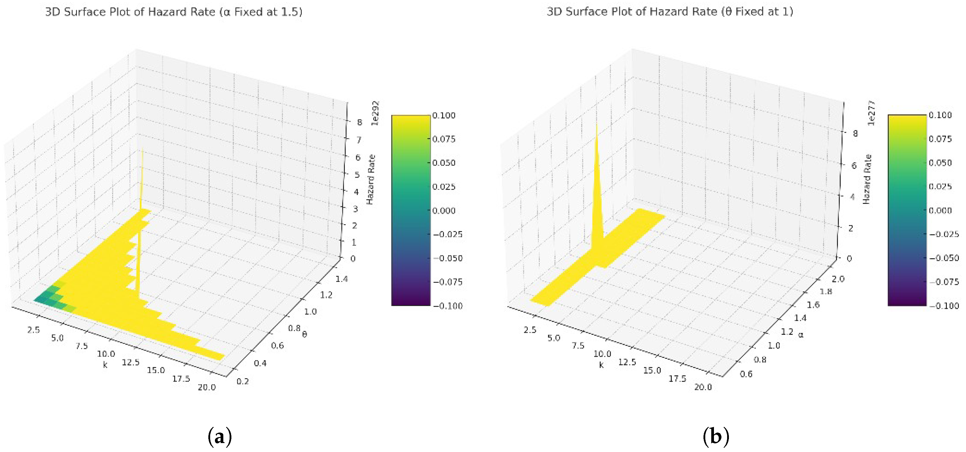
Figure 3 and Figure 4 show the behavior of the pmf and the hazard rate function respectively of the DRLD2 for different parameter values.

For the pmf of DRLD2 it can be realized from Figure 3 that for different values of the parameters, the pmf decreases, The influence of $\alpha$ and $\theta$ is summarized as follows:

• As k increases from 1 onwards, the probability $P(Y=k)$ shows a decreasing trend for all combinations of $\alpha$ and $\theta$. However, the rate of decrease and the pattern of the probabilities vary significantly with different values of $\alpha$ and $\theta$. This variation illustrates how these parameters modulate the distribution, affecting both the likelihood of higher k values and the distribution’s tail.
• The decay pattern of $P(Y=k)$ as k increases suggests that the distribution’s tail becomes thinner or heavier depending on the values of $\alpha$ and $\theta$. For some parameter combinations, the probability decreases more sharply, indicating a thinner tail. In contrast, other combinations show a more gradual decrease, suggesting a heavier tail and hence a higher probability of larger k values.
• Comparing curves of different colors (each representing a unique combination of $\alpha$ and $\theta$) indicates that higher values of $\alpha$ and/or $\theta$ generally result in a quicker drop-off in the probability as k increases. This suggests that larger values of these parameters make higher k values less likely, potentially due to the increased spread or dispersion introduced by $\alpha$ and the rate of decrease in probability mass with k influenced by $\theta$.
• The product term in the pmf for k > 0 accumulates the effect of all previous k values, introducing a dependence that shapes the overall distribution. The gradual decrease for k > 1 highlights the cumulative impact of preceding probabilities, emphasizing the distribution’s memory of past values. This effect is particularly noticeable in distributions where the probabilities do not drop to near-zero immediately, illustrating the balance between the likelihood of consecutive events.

In summary, the plot and the behavior of $P(Y=k)$ underscore the critical roles of $\alpha$ and $\theta$ in determining the distribution’s characteristics. The parameters not only influence the initial probabilities but also significantly impact the distribution’s long-tail behavior, with implications for how likely higher k values are under different conditions.

The unimodality property of the DRLD1 and DRLD2 distribution, as well as the decreasing hazard rate curve, are consistent with the characteristics of the continuous RL distribution, see [19].

Figure 4 represents the hazard rate behavior for the DRLD2 under different parameter values. In plot (a) where $\alpha$ is fixed at 1, the hazard rate is plotted against $\theta$ and k. The color gradient represents the magnitude of the hazard rate, with red being higher and blue being lower. This plot shows a more pronounced curve in the surface as $\theta$ increases, indicating that the hazard rate is more sensitive to changes in $\theta$ than to changes in $\alpha$ from the next plot (b). As $\theta$ increases, for a given value of k, the hazard rate decreases, suggesting that the parameter $\theta$ has an inverse relationship with the hazard rate.

In plot (b) where $\theta$ is fixed at 1, the hazard rate is shown as a function of $\alpha$ and k. Again, the color gradient from red to blue indicates a decrease in the hazard rate value. The surface plot shows that as k increases, the hazard rate decreases smoothly without any abrupt changes. For a fixed k, as $\alpha$ increases, the hazard rate decreases as well, which can be observed from the gradient of the surface.

The behavior of the hazard rate in these plots can point out the reliability of a system, where a lower hazard rate suggests a lesser likelihood of failure over time. The exact interpretation would depend on the context of the parameters $\alpha ,\theta$, and k, which could represent physical properties or design parameters in an engineering system.

Understanding these relationships can help in designing systems with desired reliability characteristics or in making predictions about system longevity or failure rates. For a more detailed analysis, it would be necessary to know the specific context and definitions of these parameters. Consequently, finding the estimated values of these parameters will lead to a better understanding and prediction of the system’s reliability and failure times. Hence, our next step is to use statistical inference to observe classical and Bayesian estimations for the model parameters.

3. Statistical Functions

In this section, statistical functions such as Quantile, moments, skewness, kurtosis, and ordered statistics are discussed for both discrete analogs of RLD.

3.1. Quantile Function

Due to the complexity of the CDF of DRLD1 and DRLD2, isolating k in the expression of $\omega \left(\alpha ,\theta ,k\right)$ analytically is non-trivial and likely not possible to be exact due to the nature of the expression involving both exponential and rational terms in k. Instead of an exact analytical expression, one can use approximations or numerical methods for practical applications. See

Table 1. Statistics for DLRD1 samples.

($\mathit{\alpha },\mathit{\theta }$)	${\mathit{Q}}_1$	Median	${\mathit{Q}}_3$	Mean	Variance	Skewness	Kurtosis	Range
(0.30, 0.80)	0.00	0.00	0.00	0.1906	0.1543	1.5755	3.4821	0–1
(1.50, 0.50)	2.00	3.00	4.00	3.0135	1.1724	−0.3520	2.8274	0–6
(1.00, 0.50)	2.00	2.00	3.00	2.3541	0.8954	−0.2713	2.7926	0–5
(0.20, 0.40)	0.00	1.00	1.00	0.8416	0.3669	0.0978	2.6259	0–3
(0.60, 0.60)	1.00	1.00	2.00	1.2112	0.4552	−0.0750	2.5224	0–3

for some quantile values.

3.2. Moments

Moments are important statistical functions. They provide comprehensive information about the shape and characteristics of a probability distribution and have many applications in quality control, risk management, and environmental studies among others. To find the moments for the DRLD1, assume two non-negative random variables k∼$DRLD1\left(\alpha ,\theta \right)$, and l∼$DRLD2\left(\alpha ,\theta \right)$. The sth moment, say ${\mu }_s^{\prime }$ and ${{\mu }^{*}}_s^{\prime }$ for DRLD1 and DRLD2 can be expressed, respectively, as follows:

$${\mu }_s^{\prime }=\sum _{k=0}^{\infty }{k}^s\left[e^{-\omega \left(\alpha ,\theta ,k\right)}-e^{-\omega \left(\alpha ,\theta ,k+1\right)}\right].$$

(13)

and

$${{\mu }^{*}}_s^{\prime }=\sum _{l=0}^{\infty }{l}^{s}P(Y=l).$$

(14)

where $P(Y=l)$ is defined by Equation (11). An exact expression for the sth moment cannot be derived, therefore the Matlab (R2023a) software is useful for numerically evaluating the moment. Table 1 and

Table 2. Statistics for DLRD2 samples.

($\mathit{\alpha },\mathit{\theta }$)	${\mathit{Q}}_1$	Median	${\mathit{Q}}_3$	Mean	Variance	Skewness	Kurtosis	Range
(0.30, 0.80)	0.00	1.00	2.00	1.25	3.58	2.29	9.67	0–15
(1.50, 0.50)	0.00	1.00	1.00	0.51	0.27	0.16	1.59	0–3
(1.00, 0.50)	0.00	0.00	1.00	0.51	0.29	0.76	7.56	0–7
(0.20, 0.40)	0.00	1.00	1.00	0.82	1.80	3.58	21.75	0–16
(2.00, 3.00)	0.00	1.00	2.00	1.36	3.91	2.14	9.18	0–17
(3.50, 0.50)	0.00	1.00	1.00	0.51	0.25	−0.01	1.07	0–2
(4.00, 0.50)	0.00	1.00	1.00	0.50	0.25	0.01	1.06	0–2

explore some functions like the mean, variance, skewness (SK), and kurtosis (Kt) for different values of $\alpha$ and $\theta$ for DRLD1 and DRLD2, respectively. It can be noticed that the DRLD1 distribution is appropriate for modeling under-dispersed data since in this model the variance is smaller than the mean, which is the case with some standard classical discrete distributions. In addition, the positive and negative skewness values show that this distribution can be skewed to the right or left. Also, a minimal skew value that tends to zero indicates a possible symmetry curve for the pmf. The statistics for the DRLD2 indicate the suitability of this distribution to model both over and under-dispersed data since the variance can be greater and less than the mean. For different parameter values, the skewness can be positive and negative and some values are small enough to ensure a symmetric pattern of the pmf. A higher kurtosis is an indicator of substantial tail risk and are potential outliers compared to a normal distribution. One can realize the distribution changes by varying $\theta$ and $\alpha$.

3.3. Order Statistics

Let $Z_1,Z_2,\dots ,Z_n$ be a random sample with the DRLD1 and $Z_{1:n},Z_{2:n},\dots ,Z_{n:n}$ denote the corresponding order statistics. Then, the CDF of $ith$ order statistics at the value z can be written as follows

$$F_{i:n}\left(z;\alpha ,\theta \right)=\sum _{i=1}^n\left(\begin{array}{c}n\\ m\end{array}\right){\left[F_i\left(z;\alpha ,\theta \right)\right]}^m{\left[1-F_i\left(z;\alpha ,\theta \right)\right]}^{n-m}.$$

(15)

By using the negative Binomial theorem, we have

$$F_{i:n}\left(z;\alpha ,\theta \right)=\sum _{i=1}^n\sum _{j=1}^{n-m}\left(\begin{array}{c}n\\ m\end{array}\right){\left(\begin{array}{c}n-m\\ j\end{array}\right)\left(-1\right)}^j{\left[F_i\left(z;\alpha ,\theta \right)\right]}^{m+j}.$$

(16)

Therefore,

$$F_{i:n}\left(z;\alpha ,\theta \right)=\sum _{i=1}^n\sum _{j=1}^{n-m}\left(\begin{array}{c}n\\ m\end{array}\right){\left(\begin{array}{c}n-m\\ j\end{array}\right)\left(-1\right)}^j{\left[1-e^{-\omega \left(\alpha ,\theta ,k+1\right)}\right]}^{m+j}.$$

(17)

Consequently, the pmf of the ith order statistic under the DRLD1 can be derived and expressed as follows

$$f_{i:n}\left(z;\alpha ,\theta \right)=\sum _{i=1}^n\sum _{j=1}^{n-m}\left(\begin{array}{c}n\\ m\end{array}\right){\left(\begin{array}{c}n-m\\ j\end{array}\right)\left(-1\right)}^j{\left[e^{-\omega \left(\alpha ,\theta ,k\right)}-e^{-\omega \left(\alpha ,\theta ,k+1\right)}\right]}^{m+j}.$$

So, the $rth$ moments of $z_{i:n}$ can be written as follows

$$E(Z_{i:n}^r)=\sum _{z=0}^{\infty }\sum _{i=1}^n\sum _{j=1}^{n-m}\left(\begin{array}{c}n\\ m\end{array}\right){\left(\begin{array}{c}n-m\\ j\end{array}\right)\left(-1\right)}^j{z}^r{\left[e^{-\omega \left(\alpha ,\theta ,k\right)}-e^{-\omega \left(\alpha ,\theta ,k+1\right)}\right]}^{m+j}.$$

In a similar argument, the order statistics under the DRLD2 can be obtained by using Equations (10) and (11).

4. Maximum Likelihood Estimation

In this part of the study, we calculate the undetermined parameters for both versions of the DRLD distribution by applying the Maximum Likelihood Estimation (MLE) approach. To determine the required estimators, we use numerical methods, specifically adopting the well-known Newton–Raphson method for the numerical computation.

Let $x_1,\dots ,x_n$ represent a random sampling from DRLD1. From the pmf in Equation (5), the log likelihood function is given by:

$$\ell \left(\alpha ,\theta \right)=\sum _{k=1}^n\log (e^{-\omega \left(\alpha ,\theta ,k\right)}-e^{-\omega \left(\alpha ,\theta ,k+1\right)})$$

The Maximum Likelihood Estimators (MLEs) for the parameters $\alpha$ and $\theta$ are derived by calculating the partial derivatives of the likelihood function $\ell \left(\alpha ,\theta \right)$ for $\alpha$ and $\theta$, respectively. These equations are then set to zero, and the resulting system of equations is solved numerically to obtain the estimations.

$$\frac{\partial \ell \left(\alpha ,\theta \right)}{\partial \alpha }=\sum _{k=1}^n\frac{{-{\omega }_{\alpha }\left(\alpha ,\theta ,k\right)e}^{-\omega \left(\alpha ,\theta ,k\right)}+{{\omega }_{\alpha }\left(\alpha ,\theta ,k+1\right)e}^{-\omega \left(\alpha ,\theta ,k+1\right)}}{e^{-\omega \left(\alpha ,\theta ,k\right)}-e^{-\omega \left(\alpha ,\theta ,k+1\right)}}=0$$

(18)

$$\frac{\partial \ell \left(\alpha ,\theta \right)}{\partial \theta }=\sum _{k=1}^n\frac{{-{\omega }_{\theta }\left(\alpha ,\theta ,k\right)e}^{-\omega \left(\alpha ,\theta ,k\right)}+{{\omega }_{\theta }\left(\alpha ,\theta ,k+1\right)e}^{-\omega \left(\alpha ,\theta ,k+1\right)}}{e^{-\omega \left(\alpha ,\theta ,k\right)}-e^{-\omega \left(\alpha ,\theta ,k+1\right)}}=0,$$

Such that ${\omega }_{\alpha }\left(\alpha ,\theta ,k\right)=\frac{\partial \omega \left(\alpha ,\theta ,k\right)}{\partial \alpha }=-\frac{2}{\alpha }\omega \left(\alpha ,\theta ,k\right)$ and

$${\omega }_{\theta }\left(\alpha ,\theta ,k\right)=\frac{\partial \omega \left(\alpha ,\theta ,k\right)}{\partial \theta }=\frac{\theta k{e}^{\theta k}}{{\alpha }^2}\left[\frac{(1+\theta )e^{\theta k}}{1+\theta +\theta k}-1\right]\left[\frac{1}{1+\theta +\theta k}+\frac{1+k}{{\left(1+\theta +\theta k\right)}^2}\right].$$

Similarly, the MLEs of $\alpha$ and $\theta$ can be evaluated under DRLD2, in this case, the log-likelihood function can be written depending on the pmf in Equation (11) as follows:

$$\mathcal{L}\left(\alpha ,\theta \right)=\sum _{k=1}^{n}log\left(\exp \left[e^{-\omega \left(\alpha ,\theta ,k\right)}-1\right]\prod _{i=1}^{k-1}(1-\exp \left[e^{-\omega \left(\alpha ,\theta ,i\right)}-1\right])\right)$$

$$\mathcal{L}\left(\alpha ,\theta \right)=\sum _{k=1}^n\left(e^{-\omega \left(\alpha ,\theta ,k\right)}-1\right)+\sum _{k=1}^n\sum _{i=1}^{k-1}log\left[1-\exp \left(e^{-\omega \left(\alpha ,\theta ,i\right)}-1\right)\right]$$

Therefore, the partial derivatives of $\mathcal{L}\left(\alpha ,\theta \right)$ to $\alpha$ and $\theta$ are

$$\frac{\partial \mathcal{L}\left(\alpha ,\theta \right)}{\partial \alpha }=\sum _{k=1}^n-{\omega }_{\alpha }\left(\alpha ,\theta ,k\right)e^{-\omega \left(\alpha ,\theta ,k\right)}+\sum _{k=1}^n\sum _{i=1}^{k-1}\frac{{\omega }_{\alpha }\left(\alpha ,\theta ,i\right)\exp \left(e^{-\omega \left(\alpha ,\theta ,i\right)}-1\right)e^{-\omega \left(\alpha ,\theta ,i\right)}}{1-\exp \left(e^{-\omega \left(\alpha ,\theta ,i\right)}-1\right)}=0,$$

(19)

$$\frac{\partial \mathcal{L}\left(\alpha ,\theta \right)}{\partial \theta }=\sum _{k=1}^n-{\omega }_{\theta }\left(\alpha ,\theta ,k\right)e^{-\omega \left(\alpha ,\theta ,k\right)}+\sum _{k=1}^n\sum _{i=1}^{k-1}\frac{{\omega }_{\theta }\left(\alpha ,\theta ,i\right)\exp \left(e^{-\omega \left(\alpha ,\theta ,i\right)}-1\right)e^{-\omega \left(\alpha ,\theta ,i\right)}}{1-\exp \left(e^{-\omega \left(\alpha ,\theta ,i\right)}-1\right)}=0.$$

Solving the system of two nonlinear Equations (18) and (19) can only be done numerically. Numerous numerical methods have been employed in the literature; in this case, we are utilizing the Newton–Raphson method. The discussion results are presented in Section 6.

5. Bayesian Inference

In this section, we employ the Bayesian approach to determine the unknown parameters of the two discrete RL distributions. The Bayesian technique assumes that the parameters of the model are random variables adhering to a distribution known as the prior distribution. Often, prior information is not readily available, necessitating the selection of an appropriate prior. In this study, we opt for a joint conjugate prior distribution for the parameters $\alpha$ and $\theta$, referred to as the modified Lwin Prior. This prior is specified by assigning a Gamma distribution to $\alpha$ and a Pareto (I) distribution to $\theta$. Consequently,

$$\alpha \sim \mathrm{Gamma}(a_1,b_1)\mathrm{and}\theta |\alpha \sim \mathrm{Pareto}(\mathrm{I})(\alpha a_2,b_2)$$

where $a_1, a_2, b_1$, and $b_2$ are non-negative hyperparameters of the assumed distributions. Reference [20] highlighted that expressing $\theta$ conditional on $\alpha$ holds more significance than the reverse. Furthermore, they advocate that it is more pertinent to assume the prior distributions for $\alpha$ and $\theta$ as independent.

Thus, the prior distributions for $\alpha$ and $\theta$ are presented as follows:

$${\pi }_1(\alpha )=\frac{{b_1}^{a_1}}{\Gamma (a_1)}{\alpha }^{a_1-1}{e}^{-b_1\alpha },$$

$${\pi }_2(\theta |\alpha )=\frac{\alpha a_2}{\theta b_2}{(\frac{\theta }{b_2})}^{-a_2\alpha }.$$

Therefore, the joint prior function for $\alpha$ and $\theta$ is

$$\pi (\alpha ,\theta )\propto \frac{{\alpha }^{a_1}}{\theta }{e}^{-b_1\alpha }{(\frac{\theta }{b_2})}^{-a_2\alpha }$$

(20)

The joint posterior of $\alpha$ and $\theta$ under condition of data availability is given as

$$p(\alpha ,\theta |\underline{x})=\frac{1}{K}L(\underline{x}/\alpha ,\theta )\pi (\alpha ,\theta )$$

where $L(\underline{x}/\alpha ,\theta )$ is the likelihood function of the DRLD, $\pi (\alpha ,\theta )$ is the joint prior given by Equation (20), and $K=\int \int L(\underline{x}/\alpha ,\theta )\pi (\alpha ,\theta )d\alpha d\theta$.

The process of estimating the parameters for the DRLD distribution has been examined through the use of both symmetric squared error (SE) and asymmetric LINEX loss functions. An evaluation of how well the estimators perform under these loss functions was conducted via a simulation study. Criteria such as the bias and mean square error (MSE) are utilized to determine the effectiveness of the estimation techniques.

The following loss functions are employed for estimating posterior functions.

(i)

Squared error (SE) loss function: assuming SE loss function, Bayes estimation for the parameters $\alpha$ and $\theta$ are defined as the mean or expected value for the joint posterior

$${\widehat{\alpha }}_{SE}=\frac{1}{K}\int \int \alpha L(\underline{x}/\alpha ,\theta )\pi (\alpha ,\theta )d\alpha d\theta$$

$${\widehat{\theta }}_{SE}=\frac{1}{K}\int \int \theta L(\underline{x}/\alpha ,\theta )\pi (\alpha ,\theta )d\alpha d\theta$$

(21)

(ii)

LINEX loss function: under LINEX loss function, estimating parameters with Bayesian method is written as

$${\widehat{\alpha }}_{LIN}=-\frac{1}{h}\ln [\frac{1}{K}\int \int e^{-h\alpha }L(\underline{x}/\alpha ,\theta )\pi (\alpha ,\theta )d\alpha d\theta ]$$

$${\widehat{\theta }}_{LIN}=-\frac{1}{h}\ln [\frac{1}{K}\int \int e^{-h\theta }L(\underline{x}/\alpha ,\theta )\pi (\alpha ,\theta )d\alpha d\theta ],$$

(22)

where h is the value of the shape factor and it represents the orientation of asymmetry; hence, in our study we select the values of h to be 1.5 and −1.5 in the simulation analysis.

To calculate the expected values and perform the double integration required in Equations (21) and (22), it is necessary to employ numerical approaches. We have chosen to apply the Markov Chain Monte Carlo (MCMC) strategy, specifically utilizing the Gibbs sampling method, hence, we developed an appropriate R code to facilitate this process. For additional information on this technique, interested readers can consult the reference [21].

We have to discuss two cases listed below as we developed two different discretization methods on the continuous RLD.

Case 1

Utilizing the survival discretization method results in the derivation of DRLD1, whose pmf is provided by Equation (5). The corresponding joint posterior density is as follows:

$$p_1(\alpha ,\theta /\underline{x})=\frac{1}{K}\prod _{i=1}^n\left[e^{-\omega \left(\alpha ,\theta ,i\right)}-e^{-\omega \left(\alpha ,\theta ,i+1\right)}\right]\frac{{\alpha }^{a_1}}{\theta }{e}^{-b_1\alpha }{(\frac{\theta }{b_2})}^{-a_2\alpha }$$

(23)

$$=G_{\alpha }\left(a_1+1,b_1\right)\Lambda \left(\alpha ,\theta \right),$$

where, $\Lambda \left(\alpha ,\theta \right)=\frac{1}{K}{\prod }_{i=1}^n\left[e^{-\omega \left(\alpha ,\theta ,i\right)}-e^{-\omega \left(\alpha ,\theta ,i+1\right)}\right]\frac{{\theta }^{-\alpha a_2-1}}{{b_2}^{-\alpha a_2}}$, and G(.,.) denoting the Gamma distribution.

The Bayes inference for the parameters $\alpha$ and $\theta$ under SE loss function is obtained using Equation (21) and the posterior density is obtained using Equation (23)

$${\widehat{\alpha }}_{SE}=\frac{1}{K}\int \int \prod _{i=1}^n\left[e^{-\omega \left(\alpha ,\theta ,i\right)}-e^{-\omega \left(\alpha ,\theta ,i+1\right)}\right]\frac{{\alpha }^{a_1+1}}{\theta }{e}^{-b_1\alpha }{(\frac{\theta }{b_2})}^{-a_2\mathsf{\alpha }}d\alpha d\theta$$

$${\widehat{\theta }}_{SE}=\frac{1}{K}\int \int \prod _{i=1}^n\left[e^{-\omega \left(\alpha ,\theta ,i\right)}-e^{-\omega \left(\alpha ,\theta ,i+1\right)}\right]{\theta }^{-a_2\mathsf{\alpha }}{\alpha }^{a_1}{e}^{-b_1\alpha }{(b_2)}^{a_2\mathsf{\alpha }}d\alpha d\theta$$

Using the LINEX loss function, Bayesian estimation is derived from Equation (22) in conjunction with the posterior density detailed in Equation (23)

$${\widehat{\alpha }}_{LIN}=-\frac{1}{h}\ln [\frac{1}{K}\int \int \prod _{i=1}^n\left[e^{-\omega \left(\alpha ,\theta ,i\right)}-e^{-\omega \left(\alpha ,\theta ,i+1\right)}\right]\frac{{\alpha }^{a_1}}{\theta }{e}^{-{(b}_1+h)\alpha }{(\frac{\theta }{b_2})}^{-a_2\mathsf{\alpha }}d\alpha d\theta ]$$

$${\widehat{\theta }}_{LIN}=-\frac{1}{h}\ln [\frac{1}{K}\int \int \prod _{i=1}^n\left[e^{-\omega \left(\alpha ,\theta ,i\right)}-e^{-\omega \left(\alpha ,\theta ,i+1\right)}\right]\frac{{\alpha }^{a_1}}{\theta }{e}^{-b_1\alpha -h\theta }{(\frac{\theta }{b_2})}^{-a_2\mathsf{\alpha }}d\alpha d\theta ]$$

Case 2

The second discretization method of RL produces DRLD2 with the pmf presented in Equation (11), so the joint posterior density is given by

$$p_2(\alpha ,\theta /\underline{x})=\frac{1}{K}\prod _{j=1}^n\exp \left[e^{-\omega \left(\alpha ,\theta ,j\right)}-1\right]\prod _{i=1}^{j-1}(1-\exp \left[e^{-\omega \left(\alpha ,\theta ,i\right)}-1\right])\frac{{\alpha }^{a_1}}{\theta }{e}^{-b_1\alpha }{(\frac{\theta }{b_2})}^{-a_2\alpha }$$

$${=\frac{1}{K}G}_{\alpha }\left(a_1+1,b_1\right)\Psi (\alpha ,\theta )$$

where $\Psi \left(\alpha ,\theta \right)={\prod }_{j=1}^n\exp \left[e^{-\omega \left(\alpha ,\theta ,j\right)}-1\right]{\prod }_{i=1}^{j-1}(1-\exp \left[e^{-\omega \left(\alpha ,\theta ,i\right)}-1\right])\frac{{\theta }^{-a_2\alpha -1}}{{b_2}^{-a_2\alpha }}$

Bayes estimation for the parameters $\alpha$ and $\theta$ under SE loss function is given as

$${\widehat{\alpha }}_{SE}=\frac{1}{K}\int \int \prod _{j=1}^n\exp \left[e^{-\omega \left(\alpha ,\theta ,j\right)}-1\right]\prod _{i=1}^{j-1}(1-\exp \left[e^{-\omega \left(\alpha ,\theta ,i\right)}-1\right])\frac{{\alpha }^{a_1+1}}{\theta }{e}^{-b_1\alpha }{(\frac{\theta }{b_2})}^{-a_2\mathsf{\alpha }}d\alpha d\theta$$

$${\widehat{\theta }}_{SE}=\frac{1}{K}\int \int \prod _{j=1}^n\exp \left[e^{-\omega \left(\alpha ,\theta ,j\right)}-1\right]\prod _{i=1}^{j-1}(1-\exp \left[e^{-\omega \left(\alpha ,\theta ,i\right)}-1\right]){\alpha }^{a_1}{e}^{-b_1\alpha }{(\frac{\theta }{b_2})}^{-a_2\mathsf{\alpha }}d\alpha d\theta$$

With the LINEX loss function, Bayesian estimation for the parameters is obtained by:

$${\widehat{\alpha }}_{LIN}=-\frac{1}{h}\ln [\frac{1}{K}\int \int \prod _{j=1}^n\exp \left[e^{-\omega \left(\alpha ,\theta ,j\right)}-1\right]\prod _{i=1}^{j-1}(1-\exp \left[e^{-\omega \left(\alpha ,\theta ,i\right)}-1\right])\frac{{\alpha }^{a_1}}{\theta }{e}^{-{(b}_1+h)\alpha }{\left(\frac{\theta }{b_2}\right)}^{-a_2\mathsf{\alpha }}d\alpha d\theta ]$$

$${\widehat{\theta }}_{LIN}=-\frac{1}{h}\ln [\frac{1}{K}\int \int \prod _{j=1}^n\exp \left[e^{-\omega \left(\alpha ,\theta ,j\right)}-1\right]\prod _{i=1}^{j-1}(1-\exp \left[e^{-\omega \left(\alpha ,\theta ,j\right)}-1\right])\frac{{\alpha }^{a_1}}{\theta }{e}^{-b_1\alpha -h\theta }{(\frac{\theta }{b_2})}^{-a_2\mathsf{\alpha }}d\alpha d\theta ]$$

6. Simulation Analysis

Through this section, our goal is to assess how well the two discrete variants of the continuous RL distribution perform by examining the point estimation accuracy of the unknown parameters in terms of bias and MSE. Furthermore, we will compare their performance using various loss functions outlined in Section 5. We will present some noteworthy findings and outcomes after this section.

In the simulation scenario, 10,000 iterations of random samples are generated using suitable R-code. Some predetermined parameters values for $\alpha$ and $\theta$ are $\{0.5,2\}$, with a sample size $n=\{50,100,150\}$ being considered.

The simulation analysis for estimating the parameters of the two discrete analogs of RL distribution is presented in

Table 3. The MLE and the Bayesian inference for DRLD1 with estimation bias and MSE with various values of parameters.

				MLE		Bayes (SE)		Bayes (LINEX-1.5)		Bayes (LINEX 1.5)
$\mathit{\alpha }$	$\mathit{\theta }$	n		Bias	MSE	Bias	MSE	Bias	MSE	Bias	MSE
0.5	0.5	50	$\alpha$	0.2767	0.2983	0.3212	0.2058	0.4068	0.3078	0.2397	0.1283
			$\theta$	0.0082	0.0132	0.0124	0.0089	0.0207	0.0093	0.0392	0.0086
		100	$\alpha$	0.2356	0.2307	0.1285	0.0419	0.1434	0.0487	0.1136	0.0359
			$\theta$	0.0363	0.0107	−0.0113	0.0045	−0.0183	0.0044	−0.0338	0.0046
		150	$\alpha$	0.3009	0.0997	0.0808	0.0182	0.0866	0.0197	0.0751	0.0167
			$\theta$	0.0337	0.0020	−0.0104	0.0038	−0.0144	0.0037	−0.0246	0.0038
	2	50	$\alpha$	0.5566	0.3608	0.5221	0.5461	0.6359	0.7618	0.4130	0.3687
			$\theta$	−0.3494	0.1234	−0.4743	0.3857	−0.4029	0.3057	−0.5439	0.4715
		100	$\alpha$	0.5084	0.3463	0.4526	0.2419	0.4738	0.2654	0.4059	0.2168
			$\theta$	−0.3299	0.1133	−0.3927	0.1791	−0.3753	0.1629	−0.4083	0.1943
		150	$\alpha$	0.4642	0.3350	0.4105	0.1794	0.4233	0.1915	0.3955	0.1657
			$\theta$	−0.3048	0.1024	−0.3731	0.1465	−0.3596	0.1355	−0.3847	0.1562
2	0.5	50	$\alpha$	0.0949	0.0189	0.1408	0.2011	0.2307	0.2592	0.0498	0.1630
			$\theta$	−0.0359	0.0015	−0.0340	0.0024	−0.0332	0.0024	−0.0349	0.0025
		100	$\alpha$	0.0936	0.0175	0.0366	0.0458	0.0540	0.0493	0.0193	0.0432
			$\theta$	−0.0325	0.0012	−0.0328	0.0018	−0.0308	0.0018	−0.0328	0.0018
		150	$\alpha$	0.0828	0.0162	0.0199	0.0170	0.0263	0.0177	0.0135	0.0165
			$\theta$	−0.0276	0.0011	−0.0309	0.0017	−0.0302	0.0017	−0.0309	0.0017
	2	50	$\alpha$	0.4530	0.3211	0.3866	0.4378	0.5541	0.6896	0.2218	0.2658
			$\theta$	−0.1637	0.0295	−0.1801	0.0399	−0.1737	0.0376	−0.1866	0.0422
		100	$\alpha$	0.3739	0.3020	0.1408	0.0698	0.1632	0.0806	0.1182	0.0603
			$\theta$	−0.1179	0.0215	−0.1206	0.0344	−0.1520	0.0335	−0.1721	0.0415
		150	$\alpha$	0.2530	0.2695	0.0899	0.0274	0.0982	0.0298	0.0815	0.0251
			$\theta$	−0.1195	0.0176	−0.1209	0.0314	−0.1421	0.0308	−0.1621	0.0405

and

Table 4. The MLE and the Bayesian inference for DRLD2 with estimation bias and MSE with various values of parameters.

				MLE		Bayes (SE)		Bayes (LINEX-1.5)		Bayes (LINEX 1.5)
$\mathit{\alpha }$	$\mathit{\theta }$	n		Bias	MSE	Bias	MSE	Bias	MSE	Bias	MSE
0.5	0.5	50	$\alpha$	0.2661	0.2635	0.3323	0.2177	0.4237	0.3308	0.2455	0.1332
			$\theta$	0.0026	0.0145	0.0151	0.0089	0.0236	0.0094	0.0063	0.0085
		100	$\alpha$	0.2373	0.2410	0.1272	0.0432	0.1426	0.0501	0.1119	0.0371
			$\theta$	0.0377	0.0125	−0.0133	0.0048	−0.0131	0.0047	−0.0054	0.0050
		150	$\alpha$	0.3020	0.0999	0.0801	0.0185	0.0860	0.0201	0.0742	0.0169
			$\theta$	0.0339	0.0020	−0.0125	0.0020	−0.0114	0.0038	−0.0046	0.0040
	2	50	$\alpha$	0.5574	0.3163	0.4552	0.2611	0.4168	0.1873	0.2431	0.1400
			$\theta$	−0.3524	0.1254	−0.3046	0.1185	−0.2390	0.1031	−0.2154	0.0947
		100	$\alpha$	0.2587	0.2349	0.2426	0.2183	0.2045	0.1892	0.2040	0.1297
			$\theta$	−0.3340	0.1162	−0.3042	0.1020	−0.2402	0.1018	−0.2044	0.0922
		150	$\alpha$	0.1574	0.2035	0.1421	0.1750	0.1417	0.1486	0.1390	0.1136
			$\theta$	−0.3046	0.1023	−0.2380	0.0915	−0.1307	0.0901	−0.0939	0.0816
2	0.5	50	$\alpha$	0.0541	0.0109	−0.0601	0.0101	0.0914	0.0103	−0.0666	0.0101
			$\theta$	−0.0363	0.0015	−0.0391	0.0013	−0.0395	0.0013	−0.0393	0.0013
		100	$\alpha$	0.0496	0.0102	0.0479	0.0033	−0.0536	0.0035	−0.0564	0.0031
			$\theta$	−0.0330	0.0012	−0.0361	0.0009	−0.0390	0.0009	−0.0385	0.0009
		150	$\alpha$	0.0317	0.0092	−0.0398	0.0014	−0.0231	0.0014	−0.0449	0.0013
			$\theta$	−0.0288	0.0012	−0.0358	0.0008	−0.0380	0.0008	−0.0369	0.0009
	2	50	$\alpha$	0.0541	0.0109	0.0431	0.0070	0.0555	0.0114	0.0305	0.0037
			$\theta$	−0.0363	0.0015	−0.0215	0.0013	−0.0206	0.0012	−0.0223	0.0014
		100	$\alpha$	0.0496	0.0102	0.0322	0.0014	0.0352	0.0017	0.0291	0.0012
			$\theta$	−0.0330	0.0012	−0.0224	0.0012	−0.0218	0.0011	−0.0229	0.0012
		150	$\alpha$	0.0317	0.0092	0.0214	0.0013	0.0225	0.0014	0.0201	0.0011
			$\theta$	−0.0288	0.0012	−0.0244	0.0012	−0.0234	0.0011	−0.0252	0.0013

. Primary findings from the simulation study are summarized as follows:

• It is evident that the estimated parameter values approach the true values as the sample size increases. This is indicated by the reduction in both MSE and bias with larger sample sizes, demonstrating the consistency of the proposed estimators.
• When working with small sample sizes, Bayesian estimation with LINEX loss function yields the lowest MSE and bias for estimating the parameter $\theta$. In contrast, the SE loss function produces the smallest MSE and bias for estimating $\alpha$.
• For big sample sizes, LINEX loss function consistently achieves the lowest MSE and bias for the two parameters $\alpha$ and $\theta$.
• For both parameters $\alpha$ and $\theta$, the Bayesian methods generally show a different bias and MSE pattern compared to MLE. Specifically, the Bayesian SE method tends to have lower MSE than MLE in many cases, suggesting that it might provide more accurate and reliable estimates under certain conditions. For nearly all scenarios, both the LINEX and SE loss functions result in the lowest bias and MSE values across various sample sizes.
• The LINEX penalties introduce variability in the performance, with LINEX-1.5 generally resulting in higher bias and MSE for $\alpha$, especially when $\alpha =2$, suggesting a sensitivity to the loss function’s shape.
• The performance of the estimation methods varies significantly between the two parameter settings $\alpha$ and $\theta$ = 0.5 vs. 2. For instance when $\alpha$ and $\theta$ are both set to 2, the bias and MSE are generally higher compared to when they are set to 0.5. This suggests that the true values of the parameters can significantly affect the difficulty of the estimation problem.

When comparing the performance of the estimation methods for the parameters of the two DGPD analogs, several insights emerge regarding the performance of these methods across different conditions. Below are some general observations.

• Across both distributions, the Bayesian methods, particularly with the Standard Error (SE) approach, often show a lower MSE compared to the MLE, suggesting that in the context of these simulations, Bayesian methods might offer a more robust approach under certain conditions.
• The bias for parameter $\alpha$ in DRLD2 seems to have less variability across different methods and conditions compared to DRLD1. For example, in DRLD2, the bias values for $\alpha$ are generally closer to zero, especially in the Bayesian SE and LINEX (−1.5) scenarios, indicating potentially more accurate estimations. For parameter $\theta$, the bias is also generally lower in DRLD2, suggesting that the estimation methods may perform better on this distribution for $\theta$.
• The MSE values for both $\alpha$ and $\theta$ tend to be lower in DRLD2 across most methods and conditions, indicating a more precise estimation. This is particularly evident in the Bayesian SE and LINEX (−1.5) methods, where the improvement in MSE is clear.
• The impact of increasing sample size on improving bias and MSE appears to be more consistent in DRLD2 than in DRLD1, especially for the Bayesian methods. This suggests that DRLD2 may be more amenable to these estimation techniques as the sample size increases.
• The Bayesian methods, especially with SE and LINEX (−1.5), show a notable improvement in DRLD2 over DRLD1 in terms of both bias and MSE. This could be indicative of the Bayesian methods being particularly well-suited for the characteristics of DRLD2.

The comparison between the two tables highlights that DRLD2 generally allows for more accurate parameter estimation than DRLD1, as evidenced by lower bias and MSE across various methods and conditions. The improvement is particularly noticeable with Bayesian estimation methods, suggesting that these methods may be more effective for distributions with characteristics similar to DRLD2. This could be due to differences in the underlying properties of the two distributions, such as their sensitivity to sample size and the specific challenges they present for parameter estimation.

7. Real Data Examples

This section presents the analysis using a real dataset. The main goal of this section is to examine the usefulness and applicability of the proposed discrete analogs to real phenomena. The first dataset consists of the number of fires that occurred in Greece between 1 July and 31 August 1998. We only take into account fires in forest districts. We considered a sample of data with a size of 24. The minimum value is 1, the first quartile is 4, the median value is 7.5, the mean value is 6.88, the third quartile is 9, the maximum value is 12, and the variance value is 8.9. The data are as follows:

Dataset I: 4, 3, 10, 5, 4, 5, 12, 3, 8, 10, 11, 6, 1, 8, 9, 9, 4, 8, 11, 8, 6, 4, 7, 9.

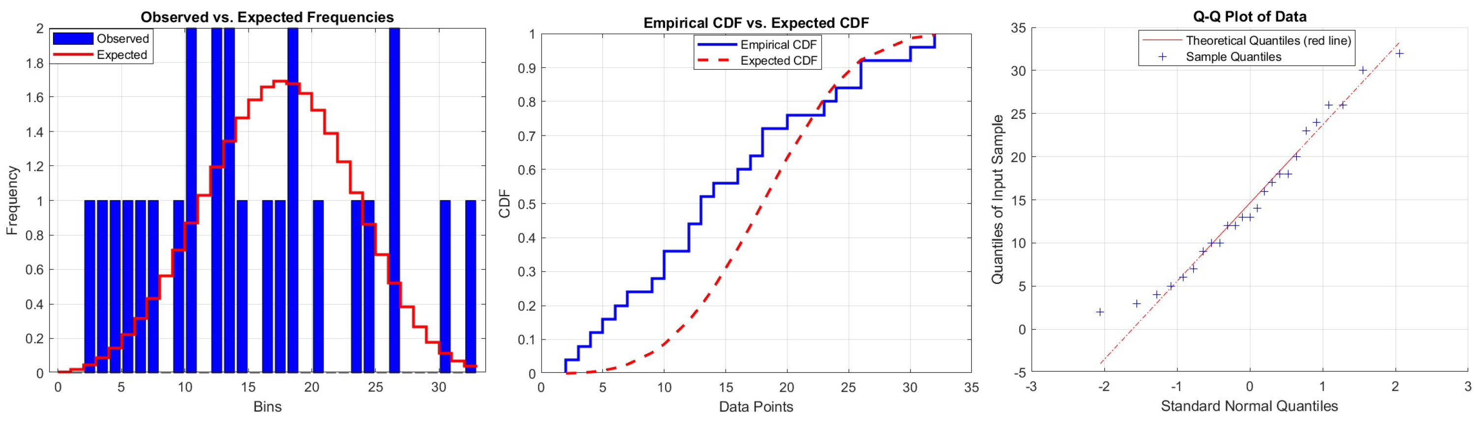
These data hae been discussed by [22]. We apply the Chi-square goodness of fit measure for testing DRLD1 with the above set of data, the results are explored in

Table 5. MLE estimate and chi-square measure for dataset I.

	Parameters	MLE	p-Value	Test Statistics
DRLD1	$\alpha$	0.1684	0.8366	0
	$\theta$	0.0849

. The observed p-value indicates the suitability of DRLD1 to fit these data. Additionally, Figure 5 illustrates the connection between observed probability distribution with the expected one, as well as the empirical CDF with the expected CDF plot, and finally the Q-Q plot.

The second dataset represents a 25-day COVID-19 data set from the United States Virgin Islands, recorded in May 2021. These data comprise daily new deaths. The data are as follows:

Dataset II: 4, 12, 3, 5, 12, 6, 9, 13, 10, 26, 32, 13, 10, 20, 18, 2, 18, 14, 24, 7, 30, 16, 26, 17, 23. The data are available on the Worldometer website at [23]. Applying the Chi-square goodness of fit test to assess the appropriateness of the DRLD2 distribution for this dataset indicates that this model is relatively well-suited for analyzing these data. The results are detailed in

Table 6. MLE estimate and chi-square measure for dataset II.

	Parameters	MLE	p-Value	Test Statistics
DRLD2	$\alpha$	0.1098	0.0853	0
	$\theta$	0.0305

. Additionally, Figure 6 displays the P-P plot, the empirical and estimated cumulative distribution functions, and the Q-Q plot.

8. Conclusions

Discrete distributions are a natural choice for modeling data that are limited to a finite or countably infinite set of values, due to their simplicity, closed-form expressions, and ability to model real-world phenomena. They are also computationally efficient and can be used to model categorical data. In this study, the author developed two new discrete analogs of the Raleigh–Lindley distribution. Their statistical properties are discussed, then estimation methods are applied to assess the performance of estimation methods for the two analogs. The simulation study illustrates the performance of MLE and Bayesian methods in estimating DRLD parameters. The choice of estimation method and the specification of the Bayesian loss function can significantly impact the bias and MSE of the estimates. These findings underscore the importance of considering the specific context of the parameter estimation problem, including the sample size and the true parameter values, when selecting an estimation approach. It was obtained that the new hazard preservation method enhances the performance of estimation methods, this is especially evident in the Bayesian estimation approaches, indicating that these techniques may be better suited for distributions that share characteristics with DRLD2. This distinction could stem from the unique attributes of the two distributions, including how they respond to changes in sample size and the particular obstacles they pose for estimating parameters. Finally, two real data examples from the environment and health fields are examined to assess the performance of each analog.

References

- Xekalaki, E. Hazard function and life distributions in discrete time. Commun. Stat. Theory Methods 1983, 12, 2503–2509. [Google Scholar] [CrossRef]
- Roy, D.; Ghosh, T. A new discretization approach with application in reliability estimation. IEEE. Trans. Reliab. 2009, 58, 456–461. [Google Scholar] [CrossRef]
- Bracquemond, C.; Gaudoin, O. A survey on discrete life time distributions. Int. J. Reliabil. Qual. Saf. Eng. 2003, 10, 69–98. [Google Scholar] [CrossRef]
- Lai, C.D. Issues concerning constructions of discrete lifetime models. Qual. Technol. Quant. Manag. 2013, 10, 251–262. [Google Scholar] [CrossRef]
- Chakraborty, S. Generating discrete analogues of continuous probability distributions—A survey of methods and constructions. J. Stat. Distrib. Appl. 2015, 2, 6. [Google Scholar] [CrossRef]
- Roy, D. The discrete normal distribution. Commun. Stat. Theor. Methods 2003, 32, 1871–1883. [Google Scholar] [CrossRef]
- Roy, D. Discrete Rayleigh distribution. IEEE. Trans. Reliab. 2004, 53, 255–260. [Google Scholar] [CrossRef]
- Al-Huniti, A.A.; Al-Dayjan, G.R. Discrete Burr type III distribution. Am. J. Math. Stat. 2012, 2, 145–152. [Google Scholar] [CrossRef]
- Bebbington, M.; Lai, C.D.; Wellington, M.; Zitikis, R. The discrete additive Weibull distribution: A bathtub-shaped hazard for discontinuous failure data. Reliab. Eng. Syst. Saf. 2012, 106, 37–44. [Google Scholar] [CrossRef]
- Barbiero, A.; Hitaj, A. Discrete half-logistic distributions with applications in reliability and risk analysis. Ann. Oper. Res. 2024, 1–31. [Google Scholar] [CrossRef]
- Sarhan, A.M. A two-parameter discrete distribution with a bathtub hazard shape. Commun. Stat. Appl. Methods 2017, 24, 15–27. [Google Scholar] [CrossRef]
- Yari, G.; Tondpour, Z. Discrete Burr XII-Gamma Distributions: Properties and Parameter Estimations. Iran. J. Sci. Technol. Trans. Sci. 2017, 42, 2237–2249. [Google Scholar] [CrossRef]
- Almetwally, E.M.; Ibrahim, G.M. Discrete Alpha Power Inverse Lomax Distribution with Application of COVID-19 Data. Int. J. Appl. Math. 2020, 9, 11–22. [Google Scholar]
- Eliwa, M.S.; Altun, E.; El-Dawoody, M.; El-Morshedy, M. A new three-parameter discrete distribution with associated INAR process and applications. IEEE Access 2020, 8, 91150–91162. [Google Scholar] [CrossRef]
- Al-Babtain, A.; Hadi, A.; Ahmed, N.; Afify, A.Z. A New Discrete Analog of the Continuous Lindley Distribution, with Reliability Applications. Entropy 2020, 22, 603. [Google Scholar] [CrossRef] [PubMed]
- Eldeeb, A.S.; Ahsan-Ul-Haq, M.; Babar, A. A Discrete Analog of Inverted Topp-Leone Distribution: Properties, Estimation and Applications. Int. J. Anal. Appl. 2021, 19, 695–708. [Google Scholar]
- Haj Ahmad, H.; Ramadan, D.A.; Almetwally, E.M. Evaluating the Discrete Generalized Rayleigh Distribution: Statistical Inferences and Applications to Real Data Analysis. Mathematics 2024, 12, 183. [Google Scholar] [CrossRef]
- Ahmad, H.H.; Almetwally, E.M. Generating optimal discrete analogue of the generalized Pareto distribution under Bayesian inference with application. Symmetry 2022, 14, 1457. [Google Scholar] [CrossRef]
- Haj Ahmad, H.; Bdair, O.M.; Naser, M.F.M.; Asgharzadeh, A. The rayleigh lindley distribution: A new generalization of rayleigh distribution with physical applications. Rev. Investig. Oper. 2023, 44, 1–18. [Google Scholar]
- Arnold, B.C.; Press, S.J. Compatible Conditional Distributions. J. Am. Stat. Assoc. 1989, 84, 152. [Google Scholar] [CrossRef]
- Karandikar, R.L. On the markov chain monte carlo (MCMC) method. Sadhana 2006, 31, 81–104. [Google Scholar] [CrossRef]
- Karlis, D.; Xekalaki, E.; Lipitakis, E.A. On some discrete valued time series models based on mixtures and thinning. In Proceedings of the Fifth Hellenic-European Conference on Computer Mathematics and Its Applications, Athens, Greece, 20–22 September 2001; pp. 872–877. [Google Scholar]
- Worldometers. Available online: https://www.worldometers.info/coronavirus (accessed on 1 June 2021).
Figure 1.
Graphs for the pmf of the DRLD1 distribution with various parameter values of and .
Figure 2.
3D surface plot of hazard rate of DRLD1 distribution. (a) , (b) .
Figure 3.
Graphs for the pmf of the DRLD2 with various parameter values of and .
Figure 4.
3D surface plot of hazard rate of DRLD2 distribution. (a) , (b) .
Figure 5.
P-P, Empirical CDF VS estimated CDF, and Q-Q plots for dataset I with DRLD1.
Figure 6.
P-P, Empirical CDF VS estimated CDF and Q-Q plots for dataset II with DRLD2.