Computational Characterization of the Multiplication Operation of Octonions via Algebraic Approaches

Abstract

A succinct and systematic form of multiplication for any arbitrary pairs of octonions is devised. A typical expression of multiplication for any pair of octonions involves 64 terms, which, from the computational and theoretical aspect, is too cumbersome. In addition, its internal relation could not be directly visualized via the expression per se. In this article, we study the internal structures of the indexes between imaginary unit octonions. It is then revealed by various copies of isomorphic structures for the multiplication. We isolate one copy and define a multiplicative structure on this. By doing so, we could keep track of all relations between indexes and the signs for cyclic permutations. The final form of our device is expressed in the form of a series of determinants, which shall offer some direct intuition about octonion multiplication and facilitate the further computational aspect of applications.

1. Introduction

The relation between algebraic systems or operations and geometry is always a fascinating topic in physics [1,2]. Their relation could be easily applied or implemented in real problems, particularly the movement of 3D objects or higher dimensional tangible or intangible objects [3,4,5]. In this research, we shall focus on the computational aspect of octonions with an aim to improve the efficiency of its computational and theoretical derivations. As we already know, there are many ways to construct octonions, such as the Fano Plane (cyclic permutations refer to the multiplication), the Cayley–Dickson construction (an octonion is regarded as a pair of quaternions), Clifford algebras, spinors, and trialities [6]. Octonions are non-commutative and non-associative but alternative (a weaker form of associativity) and power-associative [7]. A standard form of an octonion is $\overrightarrow{w}=w_0{\overrightarrow{e}}_0+w_1{\overrightarrow{e}}_1+w_2{\overrightarrow{e}}_2+w_3{\overrightarrow{e}}_3+w_4{\overrightarrow{e}}_4+w_5{\overrightarrow{e}}_5+w_6{\overrightarrow{e}}_6+w_7{\overrightarrow{e}}_7$ [8]. The product of each pair of octonions is defined via ${\displaystyle \overrightarrow{w}\overrightarrow{v}:=\sum _{i=0}^7\sum _{j=0}^7(w_i·v_j)·{\overrightarrow{e}}_i{\overrightarrow{e}}_j}$. In order to form a closed set and preserve some properties, one has to specify the product of each pair of unit octonions ${\overrightarrow{e}}_i{\overrightarrow{e}}_j$. This is carried out normally via a multiplication table, such as

Table 1. A multiplication table for ${\overrightarrow{e}}_i{\overrightarrow{e}}_j$ via rules based on modulo 7.

${\overrightarrow{e}}_i{\overrightarrow{e}}_j$	${\overrightarrow{e}}_0\equiv 1$	${\overrightarrow{e}}_1$	${\overrightarrow{e}}_2$	${\overrightarrow{e}}_3$	${\overrightarrow{e}}_4$	${\overrightarrow{e}}_5$	${\overrightarrow{e}}_6$	${\overrightarrow{e}}_7$
${\overrightarrow{e}}_0\equiv 1$	1	${\overrightarrow{e}}_1$	${\overrightarrow{e}}_2$	${\overrightarrow{e}}_3$	${\overrightarrow{e}}_4$	${\overrightarrow{e}}_5$	${\overrightarrow{e}}_6$	${\overrightarrow{e}}_7$
${\overrightarrow{e}}_1$	${\overrightarrow{e}}_1$	$-1$	${\overrightarrow{e}}_4$	${\overrightarrow{e}}_7$	$-{\overrightarrow{e}}_2$	${\overrightarrow{e}}_6$	$-{\overrightarrow{e}}_5$	$-{\overrightarrow{e}}_3$
${\overrightarrow{e}}_2$	${\overrightarrow{e}}_2$	$-{\overrightarrow{e}}_4$	$-1$	${\overrightarrow{e}}_5$	${\overrightarrow{e}}_1$	$-{\overrightarrow{e}}_3$	${\overrightarrow{e}}_7$	$-{\overrightarrow{e}}_6$
${\overrightarrow{e}}_3$	${\overrightarrow{e}}_3$	$-{\overrightarrow{e}}_7$	$-{\overrightarrow{e}}_5$	$-1$	${\overrightarrow{e}}_6$	${\overrightarrow{e}}_2$	$-{\overrightarrow{e}}_4$	${\overrightarrow{e}}_1$
${\overrightarrow{e}}_4$	${\overrightarrow{e}}_4$	${\overrightarrow{e}}_2$	$-{\overrightarrow{e}}_1$	$-{\overrightarrow{e}}_6$	$-1$	${\overrightarrow{e}}_7$	${\overrightarrow{e}}_3$	$-{\overrightarrow{e}}_5$
${\overrightarrow{e}}_5$	${\overrightarrow{e}}_5$	$-{\overrightarrow{e}}_6$	${\overrightarrow{e}}_3$	$-{\overrightarrow{e}}_2$	$-{\overrightarrow{e}}_7$	$-1$	${\overrightarrow{e}}_1$	${\overrightarrow{e}}_4$
${\overrightarrow{e}}_6$	${\overrightarrow{e}}_6$	${\overrightarrow{e}}_5$	$-{\overrightarrow{e}}_7$	${\overrightarrow{e}}_4$	$-{\overrightarrow{e}}_3$	$-{\overrightarrow{e}}_1$	$-1$	${\overrightarrow{e}}_2$
${\overrightarrow{e}}_7$	${\overrightarrow{e}}_7$	${\overrightarrow{e}}_3$	${\overrightarrow{e}}_6$	$-{\overrightarrow{e}}_1$	${\overrightarrow{e}}_5$	$-{\overrightarrow{e}}_4$	$-{\overrightarrow{e}}_2$	$-1$

, ${\overrightarrow{e}}_i\circ {\overrightarrow{e}}_{i+1}:={\overrightarrow{e}}_{i+3}$ [9], and the unit octonions ${\overrightarrow{e}}_j$ [10].

Though it is clearly specified, the real computation will concern an expansion of 64 terms in order to rearrange them into a standard form of an octonion: $\overrightarrow{w}\overrightarrow{v}:=$.

$$\begin{array}{cc}\hfill & (w_0{v}_0-w_1{v}_1-w_2{v}_2-w_3{v}_3-w_4{v}_4-w_5{v}_5-w_6{v}_6-w_7{v}_7){\overrightarrow{e}}_0\hfill \\ \hfill +& (w_0{v}_1+w_1{v}_0+w_2{v}_4+w_3{v}_7+w_5{v}_6-w_4{v}_2-w_6{v}_5-w_7{v}_3){\overrightarrow{e}}_1\hfill \\ \hfill +& (w_0{v}_2+w_2{v}_0+w_3{v}_5+w_4{v}_1+w_6{v}_7-w_1{v}_4-w_5{v}_3-w_7{v}_6){\overrightarrow{e}}_2\hfill \\ \hfill +& (w_0{v}_3+w_3{v}_0+w_4{v}_6+w_5{v}_2+w_7{v}_1-w_1{v}_7-w_2{v}_5-w_6{v}_4){\overrightarrow{e}}_3\hfill \\ \hfill +& (w_0{v}_4+w_4{v}_0+w_1{v}_2+w_5{v}_7+w_6{v}_3-w_2{v}_1-w_3{v}_6-w_7{v}_5){\overrightarrow{e}}_4\hfill \\ \hfill +& (w_0{v}_5+w_5{v}_0+w_2{v}_3+w_6{v}_1+w_7{v}_4-w_1{v}_6-w_3{v}_2-w_4{v}_7){\overrightarrow{e}}_5\hfill \\ \hfill +& (w_0{v}_6+w_6{v}_0+w_1{v}_5+w_3{v}_4+w_7{v}_2-w_2{v}_7-w_4{v}_3-w_5{v}_1){\overrightarrow{e}}_6\hfill \\ \hfill +& (w_0{v}_7+w_7{v}_0+w_1{v}_3+w_2{v}_6+w_4{v}_5-w_3{v}_1-w_5{v}_4-w_6{v}_2){\overrightarrow{e}}_7\hfill \end{array}$$

Even if one could put up with this expression, it will become unbearable when an extra octonion is involved in the product, in which there will be 512 terms to be rearranged, and the resulting coefficient of each unit octonion will contain 64 terms. The main idea of this article is to find the intrinsic relations between these indexes so as to simplify the representations into a summarized and manageable form (see Theorems 1 and 3). The development of quaternions and octonions has lasted for centuries [11,12]. Their interaction has also been studied for a long time, particularly their multiplication operators [13]. To overcome the lengthy expression of multiplication between two octonions and obtain some succinct expressions, we study the internal relation between the terms and express them in a much more manageable form, which shall facilitate the cumbersome computational aspect of operations regarding octonions. Though some applications for octonions are associated with quaternion counterparts [14,15], there are more advanced and modern applications [16] that are worth investigating if our device is adopted. It also has some intrinsic or general properties in common with other algebras from the perspectives of algebraic mapping [17].

Based on the octonionic product rule ${\overrightarrow{e}}_i\circ {\overrightarrow{e}}_{i+1}:={\overrightarrow{e}}_{i+3}$, the indexes for the unit octonions $\{{\overrightarrow{e}}_1,{\overrightarrow{e}}_2,\cdots ,{\overrightarrow{e}}_7\}$ are classified into seven cyclic permutation groups $[1]\equiv \{1,2,4\}, [2]\equiv \{2,3,5\}, [3]\equiv \{3,4,6\}$, $[4]\equiv \{4,5,7\}, [5]\equiv \{5,6,8\}, [6]\equiv \{6,7,9\}$, and $[7]\equiv \{7,8,10\}$. Each group has its distinct sum: $7,10,13,16,19,22$, and 25, respectively. We identify them with a pair of values: sum and absolute difference. We then associate them with a function $Lab$ to recover the label of its group, i.e., 1 to 7. Then, we study the relation between them, particularly their algebraic identities. In addition, the multiplicative octonion after the product of two octonions is identified via two parts:the unsigned unit octonion and the signed one. The former part is captured by the function $PM$, while the second part is captured by a counting-swap function $\#s$ and an odd-even function $ϵ$, which represents the cyclic action. Their results are mainly summarized in

Table 2. Transitional computation table: In the table, $\left[n\right]=\{n,n+1,n+3\}$.

n	$\left[\mathit{n}\right]$	$\left[\left[\mathit{n}\right]\right]=\{\overline{\mathit{b}}=(\mathit{p},\mathit{q}):\mathit{p},\mathit{q}\in \left[\mathit{n}\right],\mathit{p}\ne \mathit{q}\}$	$\{(\mathit{p}+\mathit{q},{\overline{\mathit{b}}}^{*}-{\overline{\mathit{b}}}_{*}):\mathit{p},\mathit{q}\in \left[\mathit{n}\right],\mathit{p}\ne \mathit{q}\}$	$\mathit{\sigma }\left(\mathit{n}\right)$
1	$\{1,2,4\}$	$\left\{\right(1,2),(2,4),(1,4),(2,1),(4,2),(4,1\left)\right\}$	$\left\{\right(3,1),(6,2),(5,3\left)\right\}$	7
2	$\{2,3,5\}$	$\left\{\right(2,3),(3,5),(2,5),(3,2),(5,3),(5,2\left)\right\}$	$\left\{\right(5,1),(8,2),(7,3\left)\right\}$	10
3	$\{3,4,6\}$	$\left\{\right(3,4),(4,6),(3,6),(4,3),(6,4),(6,3\left)\right\}$	$\left\{\right(7,1),(10,2),(9,3\left)\right\}$	13
4	$\{4,5,7\}$	$\left\{\right(4,5),(5,7),(4,7),(5,4),(7,5),(7,4\left)\right\}$	$\left\{\right(9,1),(12,2),(11,3\left)\right\}$	16
5	$\{5,6,8\}$	$\left\{\right(5,6),(6,8),(5,8),(6,5),(8,6),(8,5\left)\right\}$	$\left\{\right(11,1),(14,2),(13,3\left)\right\}$	19
6	$\{6,7,9\}$	$\left\{\right(6,7),(7,9),(6,9),(7,6),(9,7),(9,6\left)\right\}$	$\left\{\right(13,1),(16,2),(15,3\left)\right\}$	22
7	$\{7,8,10\}$	$\left\{\right(7,8),(8,10),(7,10),(8,7),(10,8),(10,7\left)\right\}$	$\left\{\right(15,1),(18,2),(17,3\left)\right\}$	25

and

Table 3. Compatible combinations of solutions.

$\mathit{x}=1$	${\mathit{\lambda }}_1(\mathit{p},\mathit{q})$	${\mathit{R}}_1\stackrel{{\mathit{\eta }}^{-1}}{\equiv }{\mathit{M}}_1$	${\mathit{R}}_2\stackrel{{\mathit{\eta }}^{-1}}{\equiv }{\mathit{M}}_2$	${\mathit{R}}_3\stackrel{{\mathit{\eta }}^{-1}}{\equiv }{\mathit{M}}_3$	$\mathit{P}\mathit{M}$//${\mathit{U}}_7\circ \mathit{P}\mathit{M}$
${(p,q)}_{*}=1$	$-9$	$(2,1)\stackrel{{\eta }^{-1}}{\equiv }(2,1)$	$(7,5)\stackrel{{\eta }^{-1}}{\equiv }(7,5)$	$(6,3)\stackrel{{\eta }^{-1}}{\equiv }(6,3)$	$4//4$
${(p,q)}_{*}=2$	$-8$	$(3,2)\stackrel{{\eta }^{-1}}{\equiv }(3,2)$	$(8,6)\stackrel{{\eta }^{-1}}{\equiv }(1,6)$	$(7,4)\stackrel{{\eta }^{-1}}{\equiv }(7,4)$	$5//5$
${(p,q)}_{*}=3$	$-7$	$(4,3)\stackrel{{\eta }^{-1}}{\equiv }(4,3)$	$(9,7)\stackrel{{\eta }^{-1}}{\equiv }(2,7)$	$(8,5)\stackrel{{\eta }^{-1}}{\equiv }(1,5)$	$6//6$
${(p,q)}_{*}=4$	$-6$	$(5,4)\stackrel{{\eta }^{-1}}{\equiv }(5,4)$	$(10,8)\stackrel{{\eta }^{-1}}{\equiv }(3,1)$	$(9,6)\stackrel{{\eta }^{-1}}{\equiv }(2,6)$	$7//7$
${(p,q)}_{*}=5$	$-5$	$(6,5)\stackrel{{\eta }^{-1}}{\equiv }(6,5)$	$(11,9)\stackrel{{\eta }^{-1}}{\equiv }(4,2)$	$(10,7)\stackrel{{\eta }^{-1}}{\equiv }(3,7)$	$8//1$
${(p,q)}_{*}=6$	$-4$	$(7,6)\stackrel{{\eta }^{-1}}{\equiv }(7,6)$	$(12,10)\stackrel{{\eta }^{-1}}{\equiv }(5,3)$	$(11,8)\stackrel{{\eta }^{-1}}{\equiv }(4,1)$	$9//2$
${(p,q)}_{*}=7$	$-3$	$(8,7)\stackrel{{\eta }^{-1}}{\equiv }(1,7)$	$(13,11)\stackrel{{\eta }^{-1}}{\equiv }(6,4)$	$(12,9)\stackrel{{\eta }^{-1}}{\equiv }(5,2)$	$10//3$
${(p,q)}_{*}=8$	$-2$	$(9,8)$	$(14,12)$	$(13,10)$	$11//4$
${(p,q)}_{*}=9$	$-1$	$(10,9)$	$(15,13)$	$(14,11)$	$12//5$
$x=2$	${\lambda }_2(p,q)$	${({(r,s)}^{*},{(r,s)}_{*})}_{21}$	${({(r,s)}^{*},{(r,s)}_{*})}_{22}$	${({(r,s)}^{*},{(r,s)}_{*})}_{23}$	$PM$//$U_7\circ PM$
${(p,q)}_{*}=1$	$-13$	$(-2,-3)$	$(3,1)$	$(2,-1)$	$0//7$
${(p,q)}_{*}=2$	$-12$	$(-1,-2)$	$(4,2)$	$(3,0)$	$1//1$
${(p,q)}_{*}=3$	$-11$	$(0,-1)$	$(5,3)$	$(4,1)$	$2//2$
${(p,q)}_{*}=4$	$-10$	$(1,0)$	$(6,4)$	$(5,2)$	$3//3$
${(p,q)}_{*}=5$	$-9$	$(2,1)$	$(7,5)$	$(6,3)$	$4//4$
${(p,q)}_{*}=6$	$-8$	$(3,2)$	$(8,6)$	$(7,4)$	$5//5$
${(p,q)}_{*}=7$	$-7$	$(4,3)$	$(7,9)$	$(8,5)$	$6//6$
${(p,q)}_{*}=8$	$-6$	$(5,4)$	$(8,10)$	$(9,6)$	$7//7$
$x=3$	${\lambda }_3(p,q)$	${({(r,s)}^{*},{(r,s)}_{*})}_{31}$	${({(r,s)}^{*},{(r,s)}_{*})}_{32}$	${({(r,s)}^{*},{(r,s)}_{*})}_{33}$	$PM$//$U_7\circ PM$
${(p,q)}_{*}=1$	$-11$	$(0,-1)$	$(5,3)$	$(4,1)$	$2//2$
${(p,q)}_{*}=2$	$-10$	$(1,0)$	$(6,4)$	$(5,2)$	$3//3$
${(p,q)}_{*}=3$	$-9$	$(2,1)$	$(7,5)$	$(6,3)$	$4//4$
${(p,q)}_{*}=4$	$-8$	$(3,2)$	$(8,6)$	$(7,4)$	$5//5$
${(p,q)}_{*}=5$	$-7$	$(4,3)$	$(9,7)$	$(8,5)$	$6//6$
${(p,q)}_{*}=6$	$-6$	$(5,4)$	$(10,8)$	$(9,6)$	$7//7$
${(p,q)}_{*}=7$	$-5$	$(6,5)$	$(11,9)$	$(10,7)$	$8//1$

. With these settings and their related properties, we could then define the multiplication for each pair of octonions $\overrightarrow{u}{\times }_8\overrightarrow{v}$. The main idea is to find the intrinsic relations between the cyclic groups $[1],[2],...,[7]$ in order to keep track of the action between all indexes. Such representations could facilitate our intuitive comprehension of an octonionic product.

2. Theoretical Statements and Derivations

For any given non-negative paired integers $\overline{b}=(p,q)\in {\mathbb{N}}^2$, we use ${\overline{b}}^{*}$ (or ${(p,q)}^{*}$) and ${\overline{b}}_{*}$ (or ${(p,q)}_{*}$) to denote $max\{p,q\}$ and $min\{p,q\}$, respectively.

In the table, $\sigma (n)$ denotes the sum of all values in $[n]$.

Definition 1. 

Define ${\displaystyle Lab:\bigcup _{n=1}^7[[n]]\to \{1,2,3,4,5,6,7\}}$ by

$$Lab(p,q):=\left\{\begin{array}{cc}{(p,q)}^{*}-1\hfill & ,\mathit{if}{(p,q)}^{*}-{(p,q)}_{*}=1;\hfill \\ {(p,q)}^{*}-3\hfill & ,\mathit{if}{(p,q)}^{*}-{(p,q)}_{*}=2\mathit{or}{(p,q)}^{*}-{(p,q)}_{*}=3,\hfill \end{array}\right.$$

where $[[n]]$ is defined in Table 2.

$Lab(p,q)$ (also denoted by $l(a,b)$) will recover the group to which the pair $(p,q)$ belong. This piecewise function could be further characterized via the following equivalent functions.

Claim 1. 

$Lab(p,q)={[{(p,q)}^{*}-{(p,q)}_{*}-\frac{5}{2}]}^2+{(p,q)}^{*}-\frac{13}{4}$.

Proof. 

The piecewise function defined in Definition 1 could be capsuled into the following equivalent function:

$$\begin{array}{cc}\hfill & Lab(p,q)=\{1-[{(p,q)}^{*}-{(p,q)}_{*}-1]\}·[1-\frac{{(p,q)}^{*}-{(p,q)}_{*}-1}{2}]·[{(p,q)}^{*}-1]\hfill \\ \hfill +& \{1-\frac{[{(p,q)}^{*}-{(p,q)}_{*}-2]·[{(p,q)}^{*}-{(p,q)}_{*}-3]}{2}\}·[{(p,q)}^{*}-3]\hfill \\ \hfill =& \frac{1}{2}·\{{[{(p,q)}^{*}-{(p,q)}_{*}]}^2+5·[{(p,q)}^{*}-{(p,q)}_{*}]+6\}·({(p,q)}^{*}-1)-\frac{1}{2}\hfill \\ \hfill ·& \{{[{(p,q)}^{*}-{(p,q)}_{*}]}^2+5·[{(p,q)}^{*}-{(p,q)}_{*}]+4\}·({(p,q)}^{*}-3)\hfill \\ \hfill =& {[{(p,q)}^{*}-{(p,q)}_{*}]}^2-5·[{(p,q)}^{*}-{(p,q)}_{*}]+{(p,q)}^{*}+3={[{(p,q)}^{*}-{(p,q)}_{*}-\frac{5}{2}]}^2+{(p,q)}^{*}-\frac{13}{4}.\hfill \end{array}$$

 □

Example 1. 

$Lab(5,8)=Lab(8,5)={(8-5-\frac{5}{2})}^2+8-\frac{13}{4}=5$ and $Lab(10,8)=Lab(8,10)={(10-8-\frac{5}{2})}^2+10-\frac{13}{4}=7$.

Corollary 1. 

$Lab(p,q)=\left[\begin{array}{c}{(p,q)}^{*},{(p,q)}_{*},1\end{array}\right]\left[\begin{array}{ccc}1& -1& -2\\ -1& 1& \frac{5}{2}\\ -2& \frac{5}{2}& 3\end{array}\right]\left[\begin{array}{c}{(p,q)}^{*}\\ {(p,q)}_{*}\\ 1\end{array}\right].$

Definition 2. 

$\#s(\overline{h})$ is defined by the lowest number of swapping instances with respect to the neighboring elements in the vector $\overline{h}$ in order to coincide with its ascending vector $\overline{k}$.

Example 2. 

$\#s((8,5,2))$ will be computed by the number of swapping from $(8,5,2)$ to $(8,2,5)$, from $(8,2,5)$ to $(2,8,5)$, and from $(2,8,5)$ to (2,5,8). Hence, $\#s((8,5,2))=3$.

Let $ϵ$ denote the characteristic function for even and odd non-negative integers (1 for even integers, including 0, and $-1$ for odd integers). Let $sg$ denote the sign function (1 for non-negative numbers and $-1$ for negative numbers).

Claim 2. 

$ϵ(\#s(n_1,n_2,n_3))=sg((n_2-n_1)·(n_3-n_2)·(n_3-n_1))$, where $n_1,n_2,n_3\in \mathbb{N}$ and $n_i\ne n_j$ for all $1\le i<j\le 3$.

Proof. 

There are six possible cases to be considered:

• $n_1<n_2<n_3$: Then, $ϵ(\#s(n_1,n_2,n_3))=ϵ(0)=1$ and $sg((n_2-n_1)·(n_3-n_2)·(n_3-n_1))=1$;
• $n_1<n_3<n_2$: Then, $ϵ(\#s(n_1,n_2,n_3))=ϵ(1)=-1$ and $sg((n_2-n_1)·(n_3-n_2)·(n_3-n_1))=-1$;
• $n_2<n_1<n_3$: Then, $ϵ(\#s(n_1,n_2,n_3))=ϵ(1)=-1$ and $sg((n_2-n_1)·(n_3-n_2)·(n_3-n_1))=-1$;
• $n_2<n_3<n_1$: Then, $ϵ(\#s(n_1,n_2,n_3))=ϵ(2)=1$ and $sg((n_2-n_1)·(n_3-n_2)·(n_3-n_1))=1$;
• $n_3<n_1<n_2$: Then, $ϵ(\#s(n_1,n_2,n_3))=ϵ(2)=1$ and $sg((n_2-n_1)·(n_3-n_2)·(n_3-n_1))=1$;
• $n_3<n_2<n_1$: Then, $ϵ(\#s(n_1,n_2,n_3))=ϵ(3)=-1$ and $sg((n_2-n_1)·(n_3-n_2)·(n_3-n_1))=-1$.

 □

Definition 3. 

Preliminary setting of Multiplication 1: Define ${\displaystyle PM:{\mathbb{N}}^2\to \mathbb{N}}$ by $PM(p,q):=3\ast Lab(p,q)+4-(p+q)$.

Claim 3. 

$PM(p,q)=3·{[{(p,q)}^{*}-{(p,q)}_{*}-\frac{5}{2}]}^2+2·[{(p,q)}^{*}-{(p,q)}_{*}-\frac{5}{2}]+{(p,q)}_{*}-\frac{3}{4}$.

Corollary 2. 

$PM(p,q)=PM(q,p)=3·{[{(p,q)}^{*}-{(p,q)}_{*}]}^2-13[{(p,q)}^{*}-{(p,q)}_{*}]+{(p,q)}_{*}+13$.

Corollary 3. 

$PM(p,q)=PM(q,p)=3·{[{(p,q)}^{*}-{(p,q)}_{*}-\frac{13}{6}]}^2+{(p,q)}_{*}-\frac{13}{12}$.

Corollary 4. 

$PM(p,q)=PM(q,p)=\left[\begin{array}{c}{(p,q)}^{*},{(p,q)}_{*},1\end{array}\right]\left[\begin{array}{ccc}3& -3& -\frac{13}{2}\\ -3& 3& 7\\ -\frac{13}{2}& 7& 13\end{array}\right]\left[\begin{array}{c}{(p,q)}^{*}\\ {(p,q)}_{*}\\ 1\end{array}\right].$ As one can see, the function $PM$ is completely represented by the matrix $\left[\begin{array}{ccc}3& -3& -\frac{13}{2}\\ -3& 3& 7\\ -\frac{13}{2}& 7& 13\end{array}\right]$.

Example 3. 

$PM(4,7)=PM(7,4)=3·{[7-4-\frac{5}{2}]}^2+2·[7-4-\frac{5}{2}]+4-\frac{3}{4}=5$ and $PM(8,7)=PM(7,8)=\left[\begin{array}{c}8,7,1\end{array}\right]\left[\begin{array}{ccc}3& -3& -\frac{13}{2}\\ -3& 3& 7\\ -\frac{13}{2}& 7& 13\end{array}\right]\left[\begin{array}{c}8\\ 7\\ 1\end{array}\right]=10.$

Claim 4. 

If $PM(p,q)=PM(r,s)$, then

 1. 

${(r,s)}^{*}-{(r,s)}_{*}=1\Rightarrow {(r,s)}_{*}=\lambda (p,q)+10$;

 2. 

${(r,s)}^{*}-{(r,s)}_{*}=2\Rightarrow {(r,s)}_{*}=\lambda (p,q)+14$;

 3. 

${(r,s)}^{*}-{(r,s)}_{*}=3\Rightarrow {(r,s)}_{*}=\lambda (p,q)+12$,

where

$$\lambda (p,q)=3·{[{(p,q)}^{*}-{(p,q)}_{*}]}^2-13[{(p,q)}^{*}-{(p,q)}_{*}]+{(p,q)}_{*}.$$

Proof. 

By Corollary 2, $PM(p,q)=PM(r,s)$ implies $3{[{(r,s)}^{*}-{(r,s)}_{*}]}^2-13[{(r,s)}^{*}-{(r,s)}_{*}]$$+[{(r,s)}_{*}-\lambda (p,q)]$. Let $x={(r,s)}^{*}-{(r,s)}_{*}$. Then, one has $3x^2-13x+[{(r,s)}_{*}-\lambda (p,q)]=0$, i.e.,

$$x=\frac{13\pm \sqrt{169-12[{(r,s)}_{*}-\lambda (p,q)]}}{6}.$$

If $x=1$, then $\sqrt{169-12[{(r,s)}_{*}-\lambda (p,q)]}=7$, i.e., ${(r,s)}_{*}=\lambda (p,q)+10$. If $x=2$, then $\sqrt{169-12[{(r,s)}_{*}-\lambda (p,q)]}=1$, i.e., ${(r,s)}_{*}=\lambda (p,q)+14$. If $x=3$, then $\sqrt{169-12[{(r,s)}_{*}-\lambda (p,q)]}=5$, i.e., ${(r,s)}_{*}=\lambda (p,q)+12$. □

Observe that if ${(p,q)}^{*}-{(p,q)}_{*}=1$, then $\lambda (p,q)={(p,q)}_{*}-10$; if ${(p,q)}^{*}-{(p,q)}_{*}=2$, then $\lambda (p,q)={(p,q)}_{*}-14$; if ${(p,q)}^{*}-{(p,q)}_{*}=3$, then $\lambda (p,q)={(p,q)}_{*}-12$. The feasible solutions, with $(r,s)$ not being limited to the sets 1 to 7, are demonstrated in Table 3.

There are some specifications for the table:

• $x={(p,q)}^{*}-{(p,q)}_{*}$;
• ${\lambda }_1(p,q)={(p,q)}_{*}-10$; ${\lambda }_2(p,q)={(p,q)}_{*}-14$; ${\lambda }_3(p,q)={(p,q)}_{*}-12$;
• ${({(r,s)}^{*},{(r,s)}_{*})}_{11}=({(r,s)}_{*}+1,{\lambda }_1(p,q)+10)=({(r,s)}_{*}+1,{(p,q)}_{*})=({(p,q)}_{*}+1,{(p,q)}_{*})$; ${({(r,s)}^{*},{(r,s)}_{*})}_{12}=({(r,s)}_{*}+2,{\lambda }_1(p,q)+14)=({(r,s)}_{*}+2,{(p,q)}_{*}+4)=({(p,q)}_{*}+6,{(p,q)}_{*}+4)$; ${({(r,s)}^{*},{(r,s)}_{*})}_{13}=({(r,s)}_{*}+3,{\lambda }_1(p,q)+12)=({(r,s)}_{*}+3,{(p,q)}_{*}+2)=({(p,q)}_{*}+5,{(p,q)}_{*}+2)$;
• ${({(r,s)}^{*},{(r,s)}_{*})}_{21}=({(r,s)}_{*}+1,{\lambda }_2(p,q)+10)=({(r,s)}_{*}+1,{(p,q)}_{*}-4)$; $({(r,s)}^{*},$${(r,s)}_{*}{)}_{22}=({(r,s)}_{*}+2,{\lambda }_2(p,q)+14)=({(r,s)}_{*}+2,{(p,q)}_{*})$; ${({(r,s)}^{*},{(r,s)}_{*})}_{23}=({(r,s)}_{*}+3,{\lambda }_2(p,q)+12)=({(r,s)}_{*}+3,{(p,q)}_{*}-2)$;
• ${({(r,s)}^{*},{(r,s)}_{*})}_{31}=({(r,s)}_{*}+1,{\lambda }_3(p,q)+10)=({(r,s)}_{*}+1,{(p,q)}_{*}-2)$; $({(r,s)}^{*},$${(r,s)}_{*}{)}_{32}=({(r,s)}_{*}+2,{\lambda }_3(p,q)+14)=({(r,s)}_{*}+2,{(p,q)}_{*}+2)$; ${({(r,s)}^{*},{(r,s)}_{*})}_{33}=({(r,s)}_{*}+3,{\lambda }_3(p,q)+12)=({(r,s)}_{*}+3,{(p,q)}_{*})$.

Let us apply some main abbreviations:

• $R_1\equiv {({(r,s)}^{*},{(r,s)}_{*})}_{11}:=\{({(p,q)}_{*}+1,{(p,q)}_{*}):1\le {(p,q)}_{*}\le 7\}$;
• $R_2\equiv {({(r,s)}^{*},{(r,s)}_{*})}_{12}:=\{({(p,q)}_{*}+6,{(p,q)}_{*}+4):1\le {(p,q)}_{*}\le 7\}$;
• $R_3\equiv {({(r,s)}^{*},{(r,s)}_{*})}_{13}:=\{({(p,q)}_{*}+5,{(p,q)}_{*}+2):1\le {(p,q)}_{*}\le 7\}$.

Claim 5. 

 1. 

For all $({(p,q)}_{*}+1,{(p,q)}_{*})\in R_1[PM({(p,q)}_{*}+1,{(p,q)}_{*})={(p,q)}_{*}+3]$;

 2. 

For all $({(p,q)}_{*}+6,{(p,q)}_{*}+4)\in R_2[PM({(p,q)}_{*}+6,{(p,q)}_{*}+4)={(p,q)}_{*}+3]$;

 3. 

For all $({(p,q)}_{*}+5,{(p,q)}_{*}+2)\in R_3[PM({(p,q)}_{*}+5,{(p,q)}_{*}+2)={(p,q)}_{*}+3]$.

Proof. 

By Corollary 3, one obtains $PM(a,b)=3·{({(a,b)}^{*}-{(a,b)}_{*}-\frac{13}{6})}^2+{(a,b)}_{*}-\frac{13}{12}$. By setting $a={(p,q)}_{*}+1$ and $b={(p,q)}_{*}$, one obtains $PM({(p,q)}_{*}+1,{(p,q)}_{*})={(p,q)}_{*}+3$. By the same token, we could obtain the results for the second and third statements. □

Claim 6. 

$PM([{(p,q)}_{*}+4]·(1,1)+(1,0))=PM([{(p,q)}_{*}+4]·(1,1)+(6,4))=PM([{(p,q)}_{*}$$+4]·(1,1)+(5,2))\stackrel{7}{\equiv }{(p,q)}_{*}$ for all $1\le {(p,q)}_{*}\le 7$, where $\stackrel{7}{\equiv }$ denotes mod 7.

Proof. 

It follows immediately from Claim 5. □

Claim 7. 

$U_7\circ PM({(p,q)}_{*}·(1,1)+(5,4))=U_7\circ PM({(p,q)}_{*}·(1,1)+(10,8))=U_7\circ PM({(p,q)}_{*}·(1,1)+(9,6))\stackrel{7}{\equiv }{(p,q)}_{*}$ for all $1\le {(p,q)}_{*}\le 7$.

Lemma 1. 

$U_7\circ PM({(p,q)}_{*}·(1,1)+(5,4))=U_7\circ PM({(p,q)}_{*}·(1,1)+(3,1))=U_7\circ PM({(p,q)}_{*}·(1,1)+(2,6))\stackrel{7}{\equiv }{(p,q)}_{*}$ for all $1\le {(p,q)}_{*}\le 7$.

Proof. 

It follows immediately from the definition of $U_7$ and Corollary 3. The actual computation is based on Corollary 4, and the results are shown in the rightmost column of the first part of Table 3. □

Remark 1. 

The above-mentioned results could be captured via the following respective structures: ${(p,q)}_{*}\left[\begin{array}{cc}1& 1\\ 1& 1\\ 1& 1\end{array}\right]+\left[\begin{array}{cc}1& 0\\ 6& 4\\ 5& 2\end{array}\right];{(p,q)}^{*}\left[\begin{array}{cc}1& 1\\ 1& 1\\ 1& 1\end{array}\right]$$+\left[\begin{array}{cc}-3& -4\\ 2& 0\\ 1& -2\end{array}\right];{(p,q)}_{*}\left[\begin{array}{cc}1& 1\\ 1& 1\\ 1& 1\end{array}\right]+\left[\begin{array}{cc}-1& -2\\ 4& 2\\ 3& 0\end{array}\right].$ Their relations are ${(p,q)}_{*}\left[\begin{array}{cc}1& 1\\ 1& 1\\ 1& 1\end{array}\right]+\left[\begin{array}{cc}-3& -4\\ 2& 0\\ 1& -2\end{array}\right]=[{(p,q)}_{*}-4]\left[\begin{array}{cc}1& 1\\ 1& 1\\ 1& 1\end{array}\right]+\left[\begin{array}{cc}1& 0\\ 6& 4\\ 5& 2\end{array}\right]$ and ${(p,q)}_{*}\left[\begin{array}{cc}1& 1\\ 1& 1\\ 1& 1\end{array}\right]+\left[\begin{array}{cc}-1& -2\\ 4& 2\\ 3& 0\end{array}\right]=[{(p,q)}_{*}-2]\left[\begin{array}{cc}1& 1\\ 1& 1\\ 1& 1\end{array}\right]+\left[\begin{array}{cc}1& 0\\ 6& 4\\ 5& 2\end{array}\right].$

Remark 2. 

Hence, by the previous remark, we could have three copies of isomorphic multiplicative structures. In this article, we choose the first copy of the isomorphic structure to define our original multiplication. Since the other two representations are also isomorphic to this one, one could also choose the others instead. If one does choose the other two, they shall obtain the multiplication results that differ in the indexes.

We use $(a,b)<<(c,d)$ to denote $a<c$ and $b<d$. Let the following be the case:

• $M_1\equiv \{(2,1),(3,2),(4,3),(5,4),(6,5),(7,6),(1,7)\}$;
• $M_2\equiv \{(7,5),(1,6),(2,7),(3,1),(4,2),(5,3),(6,4)\}$;
• $M_3\equiv \{(6,3),(7,4),(1,5),(2,6),(3,7),(4,1),(5,2)\}$.

Let $\delta (k,h)={(k,h)}^{*}-{(k,h)}_{*}$.

Definition 4. 

Define $\eta :M_1\cup M_2\cup M_3\to R_1\cup R_2\cup R_3$ by

$$\eta (k,h):=\left\{\begin{array}{cc}(k,h)\hfill & \mathit{if}\delta (k,h)=1;\mathit{or}[\delta (k,h)=2,\delta (k,h)\ge (7,5)];\mathit{or}[\delta (k,h)=3,\delta (k,h)\ge (6,3)];\hfill \\ (k+7,h+7)\hfill & \mathit{if}[\delta (k,h)=2,(k,h)<<(7,5)];\mathit{or}[\delta (k,h)=3,(k,h)<<(6,3)];\hfill \\ (k+7,h)\hfill & \mathit{if}\delta (k,h)\ge 4,{(k,h)}_{*}=k;\hfill \\ (k,h+7)\hfill & \mathit{if}\delta (k,h)\ge 4,{(k,h)}_{*}=h.\hfill \end{array}\right.$$

Lemma 2. 

η is a bijective function.

Proof. 

Due to the definition of $\eta$ in Definition 4, $M_1$ is isomorphic to $R_1$, $M_2$ is isomorphic to $R_2$, and $M_3$ is isomorphic to $R_3$. Since they are all disjoint, the derivation is completed. □

Let us use ${\eta }^{-1}$ to denote its inverse function. Let us use $M_1\cup M_2\cup M_3\stackrel{\eta }{\equiv }{R}_1\cup R_2\cup R_3$ to denote that $M_1\cup M_2\cup M_3$ is isomorphic to $R_1\cup R_2\cup R_3$ via $\eta$; $R_1\cup R_2\cup R_3\stackrel{{\eta }^{-1}}{\equiv }{M}_1\cup M_2\cup M_3$ is used to denote that $R_1\cup R_2\cup R_3$ is isomorphic to $M_1\cup M_2\cup M_3$ via ${\eta }^{-1}$. Some similar statements hold for their elements as well. The corresponding relation between them is shown in the first part in Table 3.

Definition 5. 

Preliminary setting of Multiplication 2: Define

$$U_7(k):=\left\{\begin{array}{cc}7\hfill & ,\mathit{if}k=0;\hfill \\ k\hfill & ,\mathit{if}1\le k\le 7;\hfill \\ k-7\hfill & ,\mathit{if}k>7.\hfill \end{array}\right.$$

Lemma 3. 

 1. 

$U_7\circ PM\circ \eta (6,5)=U_7\circ PM\circ \eta (4,2)=U_7\circ PM\circ \eta (7,3)=1$;

 2. 

$U_7\circ PM\circ \eta (7,6)=U_7\circ PM\circ \eta (5,3)=U_7\circ PM\circ \eta (4,1)=2$;

 3. 

$U_7\circ PM\circ \eta (7,1)=U_7\circ PM\circ \eta (6,4)=U_7\circ PM\circ \eta (5,2)=3$;

 4. 

$U_7\circ PM\circ \eta (2,1)=U_7\circ PM\circ \eta (7,5)=U_7\circ PM\circ \eta (6,3)=4$;

 5. 

$U_7\circ PM\circ \eta (3,2)=U_7\circ PM\circ \eta (6,1)=U_7\circ PM\circ \eta (7,4)=5$;

 6. 

$U_7\circ PM\circ \eta (4,3)=U_7\circ PM\circ \eta (7,2)=U_7\circ PM\circ \eta (5,1)=6$;

 7. 

$U_7\circ PM\circ \eta (5,4)=U_7\circ PM\circ \eta (3,1)=U_7\circ PM\circ \eta (6,2)=7$.

Proof. 

By Lemma 2, the results are presented in the first part of Table 3; by Lemma 1, one could verify the validity of these statements. □

Let $\overrightarrow{u}\ast \overrightarrow{v}$ denote the concatenation of two vectors. Let $\rho (i,j)=U_7\circ PM\circ \eta ({(i,j)}^{*},{(i,j)}_{*})$.

Lemma 4. 

 1. 

$\forall x\in M_1\cup M_2[ϵ\circ \#s(x\ast \rho (x))=-1]$;

 2. 

$\forall x\in M_3[ϵ\circ \#s(x\ast \rho (x))=1]$.

Proof. 

For the first statement, consider the set $\{x\ast \rho (x):x\in M_1\}=\{(2,1,4),(3,2,5),$$(4,3,6),(5,4,7),(6,5,1),(7,6,2),(1,7,3)\}$ and $\{x\ast \rho (x):x\in M_2\}=\{(7,5,4),(1,6,5),$$(2,7,6),(3,1,7),(4,2,1),(5,3,2),(6,4,3)\}$. Then, by Claim 2, $ϵ(\#s(n_1,n_2,n_3))=-1$, where $(n_1,n_2,n_3)$ represents an element in the set. For the second statement, consider the set $\{x\ast \rho (x):x\in M_3\}=\{(6,3,4),(7,4,5),(1,5,6),(2,6,7),(3,7,1),(4,1,2),(5,2,3)\}$. Again, by Claim 2, $ϵ(\#s(n_1,n_2,n_3))=1$. □

Definition 6. 

The index operation for the unit multiplication rule is as follows:

$${\displaystyle \overrightarrow{w}{\times }_8\overrightarrow{v}=(w_0{v}_0-\sum _{i=1}^7{w}_i{v}_i)+\sum _{i=1}^7(w_0{v}_i+w_i{v}_{)}){\overrightarrow{e}}_i+\sum _{1\le i,j\le 7}^{i\ne j}{w}_i{v}_j{(-1)}^{ϵ\circ \#s(\overline{t})}·{\overrightarrow{e}}_{\rho (i,j)},}$$

where $\rho (i,j)=U_7\circ PM\circ \eta ({(i,j)}^{*},{(i,j)}_{*})$, and $\overline{t}=(i,j,\rho (i,j))$.

Theorem 1. 

${\displaystyle \overrightarrow{w}{\times }_8\overrightarrow{v}=\sum _{n=0}^7{(-1)}^{2^n+1}·\left|\begin{array}{cc}{w}_n& 0\\ 0& v_n\end{array}\right|+}$

${\displaystyle \sum _{n=1}^7\left[\left|\begin{array}{cc}{w}_0& -w_n\\ v_0& v_n\end{array}\right|+\left|\begin{array}{cc}{w}_{U_7(n+4)}& w_{U_7(n+5)}\\ v_{U_7(n+4)}& v_{U_7(n+5)}\end{array}\right|+\left|\begin{array}{cc}{w}_{U_7(n+1)}& w_{U_7(n+3)}\\ v_{U_7(n+1)}& v_{U_7(n+3)}\end{array}\right|+\left|\begin{array}{cc}{w}_{U_7(n+2)}& w_{U_7(n+6)}\\ v_{U_7(n+2)}& v_{U_7(n+6)}\end{array}\right|\right]{\overrightarrow{e}}_n.}$

Proof. 

The first and second determinants correspond to the terms in the same parts in Definition 1. Now, we argue the other parts. By replacing ${(p,q)}_{*}$ with a variable n in Lemma 1, one obtains

$$U_7\circ PM(n+5,n+4)=U_7\circ PM(n+3,n+1)=U_7\circ PM(n+2,n+6)\stackrel{7}{\equiv }n$$

for all $1\le n\le 7$. Hence, by Lemmas 2 and 3, one obtains the set of paired (unsigned) coefficients

$$\{(n+5,n+4),(n+3,n+1),(n+2,n+6)\}$$

for each ${\overrightarrow{e}}_n$. The signs for each multiplicative combination is then decided via Lemma 4. The eventual terms are presented in the forms of the last three determinants. □

The form in Theorem 1 could be further represented by a form of the inner product (denoted by •): ${\displaystyle \overrightarrow{w}{\times }_8\overrightarrow{v}=\sum _{n=0}^7{(-1)}^{2^n+1}·(w_n·v_n)+\sum _{n=1}^7[\underset{w_n}{\overset{+}{\to }}•\underset{v_n}{\overset{+}{\to }}-\underset{w_n}{\overset{-}{\to }}•\underset{v_n}{\overset{-}{\to }}]{\overrightarrow{e}}_n\equiv \sum _{n=0}^7{(-1)}^{2^n+1}·\left|\begin{array}{cc}{w}_n& 0\\ 0& v_n\end{array}\right|}$+${\displaystyle \sum _{n=1}^7\left|\begin{array}{cc}\underset{w_n}{\overset{+}{\to }}& \underset{w_n}{\overset{-}{\to }}\\ \underset{v_n}{\overset{-}{\to }}& \underset{v_n}{\overset{+}{\to }}\end{array}\right|{\overrightarrow{e}}_n,}$ where the following is the case:

• $\underset{w_n}{\overset{+}{\to }}=(w_0,w_{U_7(n+4)},w_{U_7(n+1)},w_{U_7(n+2)})$;
• $\underset{w_n}{\overset{-}{\to }}=(-w_n,w_{U_7(n+5)},w_{U_7(n+3)},w_{U_7(n+6)})$;
• $\underset{v_n}{\overset{+}{\to }}=(v_n,v_{U_7(n+5)},v_{U_7(n+3)},v_{U_7(n+6)})$;
• $\underset{v_n}{\overset{-}{\to }}=(v_0,v_{U_7(n+4)},v_{U_7(n+1)},v_{U_7(n+2)})$.

Theorem 2. 

$\overrightarrow{w}{\times }_8\overrightarrow{v}=\overrightarrow{w}\overrightarrow{v}$.

Proof. 

By expanding the terms of $\overrightarrow{w}{\times }_8\overrightarrow{v}$ with $U_7$ and the operation of determinants, one could show that they match the terms of $\overrightarrow{w}\overrightarrow{v}$. □

Corollary 5. 

$\left|\right|\overrightarrow{w}{\times }_8\overrightarrow{v}\left|\right|=\left|\right|\overrightarrow{w}\left|\right|·\left|\right|\overrightarrow{v}\left|\right|$.

Proof. 

By Theorem 2, $\left|\right|\overrightarrow{w}{\times }_8\overrightarrow{v}\left|\right|=\left|\right|\overrightarrow{w}\overrightarrow{v}\left|\right|=\left|\right|\overrightarrow{w}\left|\right|·\left|\right|\overrightarrow{v}\left|\right|$. □

Some simple results following this theorem are as follows:

• $\overrightarrow{v}{\times }_8\overrightarrow{w}=-\overrightarrow{w}{\times }_8\overrightarrow{v}$;
• ${\displaystyle \overrightarrow{w}{\times }_8{\overrightarrow{w}}^{*}=\sum _{j=0}^7{(w_j)}^2}$, where ${\displaystyle {\overrightarrow{w}}^{*}:=w_0-\sum _{j=1}^7{w}_j·{\overrightarrow{e}}_j}$;
• ${\displaystyle \left|\right|\overrightarrow{w}\left|\right|:=\sqrt{\overrightarrow{w}{\times }_8{\overrightarrow{w}}^{*}}=\sqrt{\sum _{j=0}^7{(w_j)}^2}}$.

Theorem 3. 

${\displaystyle (\overrightarrow{w}{\times }_8\overrightarrow{v}){\times }_8\overrightarrow{z}=\sum _{m=0}^7{(-1)}^{2^m+1}·\left|\begin{array}{cc}{c}_m& 0\\ 0& z_m\end{array}\right|+\sum _{n=1}^7[\left|\begin{array}{cc}{c}_0& -c_n\\ z_0& z_n\end{array}\right|}$${\displaystyle +\sum _{j=0}^2\left|\begin{array}{cc}{c}_{U_7(n+2^j)}& c_{U_7(n+2^j+2^{2^j})}\\ z_{U_7(n+2^j)}& z_{U_7(n+2^j+2^{2^j})}\end{array}\right|]{\overrightarrow{e}}_n,}$ where ${\displaystyle c_0=\sum _{m=0}^7{(-1)}^{2^m+1}·(w_m·v_m)}$ and $c_k=\left|\begin{array}{cc}\underset{w_k}{\overset{+}{\to }}& \underset{w_k}{\overset{-}{\to }}\\ \underset{v_k}{\overset{-}{\to }}& \underset{v_k}{\overset{+}{\to }}\end{array}\right|$ for $1\le k\le 7$.

Proof. 

Suppose ${\displaystyle \overrightarrow{w}{\times }_8\overrightarrow{v}=c_0+\sum _{i=1}^7{c}_j{\overrightarrow{e}}_j}$. By Theorem 1, ${\displaystyle (\overrightarrow{w}{\times }_8\overrightarrow{v}){\times }_8\overrightarrow{z}=\sum _{m=0}^7{(-1)}^{2^m+1}·\left|\begin{array}{cc}{c}_m& 0\\ 0& z_m\end{array}\right|}$+${\displaystyle \sum _{n=1}^7\left|\begin{array}{cc}\underset{c_n}{\overset{+}{\to }}& \underset{c_n}{\overset{-}{\to }}\\ \underset{z_n}{\overset{-}{\to }}& \underset{z_n}{\overset{+}{\to }}\end{array}\right|{\overrightarrow{e}}_n=\sum _{m=0}^7{(-1)}^{2^m+1}·\left|\begin{array}{cc}{c}_m& 0\\ 0& z_m\end{array}\right|+\sum _{n=1}^7\left[\left|\begin{array}{cc}{c}_0& -c_n\\ z_0& z_n\end{array}\right|+\left|\begin{array}{cc}{c}_{U_7(n+1)}& c_{U_7(n+3)}\\ z_{U_7(n+1)}& z_{U_7(n+3)}\end{array}\right|+\left|\begin{array}{cc}{c}_{U_7(n+2)}& c_{U_7(n+6)}\\ z_{U_7(n+2)}& z_{U_7(n+6)}\end{array}\right|+\right.\left|\begin{array}{cc}{c}_{U_7(n+4)}& c_{U_7(n+5)}\\ z_{U_7(n+4)}& z_{U_7(n+5)}\end{array}\right|{\overrightarrow{e}}_n=\sum _{m=0}^7{(-1)}^{2^m+1}·\left|\begin{array}{cc}{c}_m& 0\\ 0& z_m\end{array}\right|+\sum _{n=1}^7\left[{\displaystyle \left|\begin{array}{cc}{c}_0& -c_n\\ z_0& z_n\end{array}\right|+\sum _{j=0}^2\left|\begin{array}{cc}{c}_{U_7(n+2^j)}& c_{U_7(n+2^j+2^{2^j})}\\ z_{U_7(n+2^j)}& z_{U_7(n+2^j+2^{2^j})}\end{array}\right|}\right]{\overrightarrow{e}}_n.}$ □

This theorem could be further explicitly expressed as follows:

Corollary 6. 

${\displaystyle (\overrightarrow{w}{\times }_8\overrightarrow{v}){\times }_8\overrightarrow{z}=z_0·(w_0·v_0-\sum _{i=1}^7{w}_i·v_i)-\sum _{j=1}^7{z}_j·\left|\begin{array}{cc}\underset{w_j}{\overset{+}{\to }}& \underset{w_j}{\overset{-}{\to }}\\ \underset{v_j}{\overset{-}{\to }}& \underset{v_j}{\overset{+}{\to }}\end{array}\right|+[\sum _{n=1}^7{z}_n·(w_0·v_0-\sum _{i=1}^7{w}_i·v_i)+z_0·\left|\begin{array}{cc}\underset{w_n}{\overset{+}{\to }}& \underset{w_n}{\overset{-}{\to }}\\ \underset{v_n}{\overset{-}{\to }}& \underset{v_n}{\overset{+}{\to }}\end{array}\right|+\sum _{j=1}^2{z}_{U_7(n+2^j+2^{2^j})}·\left|\begin{array}{cc}\underset{w_{U_7(n+2^j)}}{\overset{+}{\to }}& \underset{w_{U_7(n+2^j)}}{\overset{-}{\to }}\\ \underset{v_{U_7(n+2^j)}}{\overset{-}{\to }}& \underset{v_{U_7(n+2^j)}}{\overset{+}{\to }}\end{array}\right|-z_{U_7(n+2^j)}}$$·\left|\begin{array}{cc}\underset{w_{U_7(n+2^j+2^{2^j})}}{\overset{+}{\to }}& \underset{w_{U_7(n+2^j+2^{2^j})}}{\overset{-}{\to }}\\ \underset{v_{U_7(n+2^j+2^{2^j})}}{\overset{-}{\to }}& \underset{v_{U_7(n+2^j+2^{2^j})}}{\overset{+}{\to }}\end{array}\right|].$

Proof. 

It follows immediately from Theorem 3 by expanding the terms in the theorem. □

3. Applications

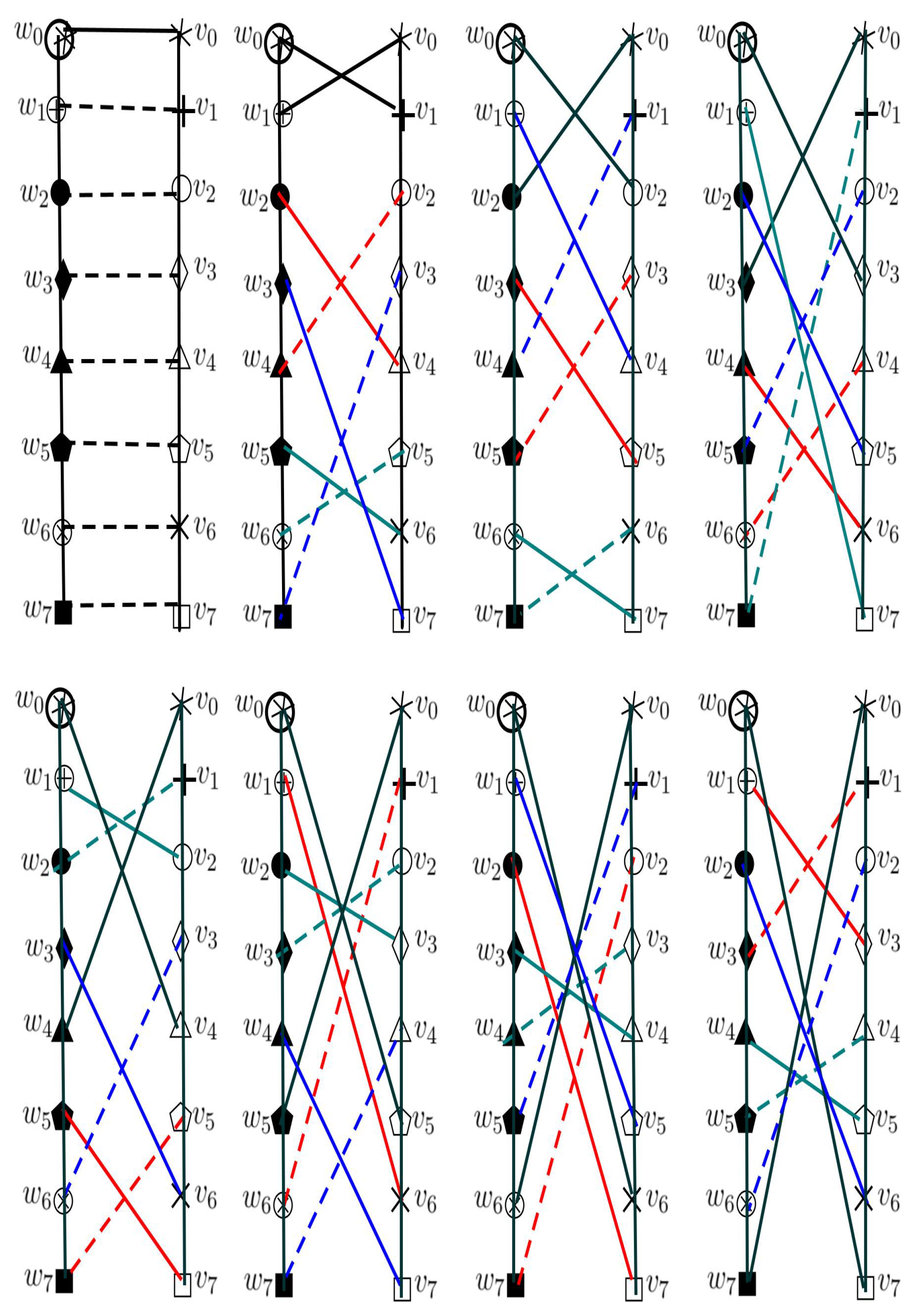
Before we embark on the application of the octonion (product), we identify our derived product structures in Theorem 1 with graphical and tree-like structures (Figure 1). This visualization should enable us in modeling the natural and social phenomenon. The benefit for this representation, either in the derived form or graphical structures, lies in its intuitive and succinct capture of high-dimensional data or analysis. Since the octonion product is non-communicative, it resembles a causal (directional) relation [18]. From Figure 1, we could summarize some properties for the kind of modeling that fits better in this representation:

• Theorem 1 reveals a structure with a sequence of bijective directional ordered trees—an explanation is offered in the caption of Figure 1;
• In principle, it fits better for ranked data, since the solid lines correspond to (or interpretable as) the relation from lower ranked values to higher ranked values;
• All relations emitted from $w_0$ and $v_0$ are positive (solid lines)—this indicates the property that the relation is definitely positive;
• The eight graphs in the figure could be used to represent eight probabilistic/deterministic states or seven states with one reference state or other similar mechanisms.

Now, we exploit our derived theorem and graphical structures to study the causality from investment (cost) to the revenue of an industry (this would diminish or even remove the temporal effect and justify the ranking approach) on a weekly basis. The provided data are sorted from the lowest value to the highest one on a weekly basis, as shown in

Table 4. Octonionic causal analysis.

Rank	Cost, Week 1	Revenue, Week 1	Cost, Week 2	Revenue, Week 2
(sunken)	$w_0=$ USD 180	$v_0=$ USD 200	USD 168	USD 189
1	$w_1=$ USD 23	$v_1=$ USD 12	USD 9	USD 21
2	$w_2=$ USD 28	$v_2=$ USD 45	USD 20	USD 32
3	$w_3=$ USD 36	$v_3=$ USD 47	USD 36	USD 40
4	$w_4=$ USD 53	$v_4=$ USD 62	USD 52	USD 55
5	$w_5=$ USD 67	$v_5=$ USD 88	USD 79	USD 65
6	$w_6=$ USD 88	$v_6=$ USD 121	USD 100	USD 81
7	$w_7=$ USD 92	$v_7=$ USD 157	USD 117	USD 132

.

There are several assumptions regarding the causal analysis:

• The sunken cost (invested) and incurred revenue (for example, annual rental income, inventory, etc.) are assigned (proportionally for one week, if the cost/revenue is calculated yearly or monthly) to the initial fixed cost (noted by $w_0$) and revenue (noted by $v_0$) assigned for the week;
• Regarding the initial values, or $w_0,v_0$, and the seven ranks (from 1 to 7), one reference state and seven probabilistic states are presented—each of which is captured by the coefficients of the seven imaginary parts of an octonion. The seven probabilistic states are distinguished by one rank, as shown in Figure 1;
• The initial cost leads to all positive increases in revenue; weekday and weekend costs lead to an (anticipated) increase in initial incurred revenue. This assumption could be amended by changing the sign of $v_0$ directly in the source data;
• For the reference state, two forces are offsetting each other: the same-rank correlation, or ${\displaystyle \sum _{n=1}^7(w_n·v_n)}$, and the initial fixed-term relation $(w_0·v_0)$. This value is quantified via ${\displaystyle |w_0·v_0-\sum _{n=1}^7(w_n·v_n)|}$, which serves as the benchmark for zero causality;
• The weighted state is evaluated via the seven probabilistic states with weights from the reference state;
• The value of the multiplication of any two values is regarded as the strength of either positive or negative causality;
• The causality between cost and revenue is revealed/sampled by three rank differences 1, 2, and 4 (for the choice of another difference, one shall consider the other 480 isomorphic octonion products), which correspond to the different colors in Figure 1;
• The strength of the causality is measured via multiplication between the cost and revenue, and its sign is determined by ascending (positive, solid lines) or descending rankings (negative, dashed lines).

We write an R program (version 4.2.2) to implement the given data in Table 4. The source codes could be fetched via https://github.com/raymingchen/Mathematics-octonion-product.git (accessed on 2 February 2024). The causal ratio for Week One is $60.61$ and Week Two is $14.61$. Obviously, Week One demonstrates a stronger causal relation wiht respect to the cost and revenue than Week Two.

4. Conclusions

A succinct and intuitive expression of the multiplication between pairs of octonions is obtained via a set of algebraic approaches. In this approach, we study the internal structures between the indexes of the octonions and find three copies of isomorphic multiplicative structures. We then singled out one and defined multiplication based on this structure. This algebraic approach keeps track of the relation between the indexes, and the final expression could be demonstrated by a series of determinants and related indexes. Such expression, with a better intuitive and manageable presentation, is equivalent to the chosen copy. It facilitates other researchers in studying the computational aspect of octonions and largely expands our capacity in the theoretical derivations of other mathematical statements. The efficacy of our new derived definition regarding the octonionic product is also witnessed by a given application and an analysis of applicability. In this research, we solely dealt with the computational aspect of octonions. Indeed, the octonionic product chosen was based on the multiplication rule ${\overrightarrow{e}}_i\circ {\overrightarrow{e}}_{i+1}={\overrightarrow{e}}_{i+3}$, which is isomorphic to another 489 multiplication rules. If one wants to construct the same formats produced here, then the new representations need to be built from scratch. We only dealt with octonionic products. If one is interested in seeking the relations between an octonionic product and a quaternionic product, then the multiplication rule for quaternions meeds to be singled out, and their relations should be studied from there. In the future, we will focus on applying these new equivalent definitions in other theoretical derivations or applicable aspects related to graphical and computational geometry [19,20]. In addition, we might also need to further derive other similar statements for other octonionic products.

References

- Snygg, J. Clifford Algebra: A Computational Tool for Physicists; Oxford University Press: Oxford, UK, 1997. [Google Scholar]
- Doran, C.; Lasenby, A. Geometric Algebra for Physicists; Cambridge University Press: Cambridge, UK, 2013. [Google Scholar]
- Vince, J. Quaternions for Computer Graphics; Springer: London, UK, 2011. [Google Scholar]
- Guterman, A.E.; Zhilina, S.A. Relation Graphs of the Sedenion Algebra. J. Math. Sci. 2021, 255, 254–270. [Google Scholar] [CrossRef]
- Conway, J.H.; Derek, A.S. On Quaternions and Octonions: Their Geometry, Arithmetic, and Symmetry; A K Peters: Natick, MA, USA, 2003. [Google Scholar]
- Baez, J. The octonions. Bull. Amer. Math. Soc. 2002, 39, 145–205. [Google Scholar] [CrossRef]
- Springer, T.A.; Veldkamp, F. Octonions, Jordan Algebras and Exceptional Groups, Springer Monographs in Mathematics; Springer: Berlin/Heidelberg, Germany, 2000. [Google Scholar]
- Killgore, P.L. The Geometry of the Octonionic Multiplication Table. Bachelor’s Thesis, Oregon State University, Corvallis, OR, USA, 2015. [Google Scholar]
- Lounesto, P. Clifford Algebras and Spinors; Cambridge University Press: Cambridge, UK, 2001. [Google Scholar]
- Yayli, Y. Unit octonions and some geometrical interpretations. Int. J. Math. Educ. Sci. Technol. 1997, 28, 749–783. [Google Scholar] [CrossRef]
- Burnside, W. Octonions: A Development of Clifford’s Bi-quaternions. Nature 1899, 59, 411–412. [Google Scholar] [CrossRef]
- Fenn, R. Quaternions and Octonions. In Geometry; Springer Undergraduate Mathematics Series; Springer: London, UK, 2001. [Google Scholar]
- Crasmareanu, M. Quaternionic Product of Circles and Cycles and Octonionic Product for Pairs of Circles. J. Math. Sci. Inform. 2022, 17, 227–237. [Google Scholar] [CrossRef]
- Dixon, G. On quaternions and octonions: Their geometry, arithmetic, and symmetry. Math. Intell. 2004, 26, 229–243. [Google Scholar] [CrossRef]
- Kharinov, M. On the Quaternion Representation for Octonion Generalization of Lorentz Boosts. J. Appl. Math. Comput. 2022, 6, 198–205. [Google Scholar]
- Li, B.; Cao, Y.; Li, Y. The Dynamics of Octonion-valued Neutral Type High-order Hopfield Neural Networks with D Operator. J. Intell. Fuzzy Syst. 2023, 44, 9599–9613. [Google Scholar] [CrossRef]
- Ferreira, B.L.; Julius, H.; Smigly, D. Commuting maps and identities with inverses on alternative division rings. J. Algebra 2024, 638, 488–505. [Google Scholar] [CrossRef]
- Chen, R.M. A direct approach of causal detection for agriculture related variables via spatial and temporal non-parametric analysis. Environ. Ecol. Stat. 2024, 31, 79–96. [Google Scholar] [CrossRef]
- Hanson, A.J. Visualizing Quaternions; Elsevier Morgan Kaufmann Publishers: Amsterdam, The Netherlands, 2006. [Google Scholar]
- Vince, J. Geometric Algebra for Computer Graphics; Springer: London, UK, 2008. [Google Scholar]
Figure 1.
A sequence of dynamic graphical (tree-like) structures identifying : Each tree structure represents the coefficient of each . The upper four tree structures correspond to the coefficients of and , while the lower four correspond to the coefficients of and , respectively. In each structure, the nodes are assigned different shapes to indicate that there are ordered vectors. Identical shapes with solid shades or circles are applied to separate the octonions and . The edges represent the linkage between nodes, in which the solid lines indicate positive relations and the dashed lines indicate negative relations. The colored lines are used to keep track of the dynamical/probabilistic changes in their relations.