Robust Consensus Modeling: Concerning Consensus Fairness and Efficiency with Uncertain Costs

Abstract

Extensive uncertainty can affect the efficiency and fairness of consensus in the consensus reaching process (CRP), but few scholars have studied consensus modeling that focuses on fairness and efficiency in uncertain environments. Additionally, the weight of the decision maker (DM) in the CRP is influenced by multiple factors. Therefore, this paper proposes robust consensus models (EFCMs) focusing on fairness and efficiency under uncertain costs to address these issues. Firstly, this paper constructs multiple uncertainty sets to describe the uncertainty of the unit adjustment cost. Secondly, the fair utility level and opinion adjustment distance are used to measure the fairness and efficiency of reaching consensus, respectively. Furthermore, this paper uses a data-driven method based on the KDE method combined with trust propagation in social networks to determine the DMs’ weights jointly. Finally, this paper also applies the proposed models to the carbon emission reduction negotiation process between the government and enterprises. The experimental results and sensitivity analysis show that the consensus cost budget and the DMs’ jealous preference behavior particularly affects the efficiency of reaching consensus, which provides a theoretical basis for solving practical decision making problems.

1. Introduction

Group decision making (GDM) is the overall process of analyzing and formulating decisions by more than one person in order to give full play to collective wisdom and to consider collective opinions, a process that allows for the expression and modification of individual and collective opinions and aims to study how to integrate the views of multiple DMs into a group view [1,2,3]. In classic GDM, the group opinion, often formed by forcibly assembling individual opinions, lacks wide recognition by decision makers (DMs), thus affecting the effectiveness of decision making and the smooth implementation of group programs. For this reason, group consensus studies have been proposed and applied to coordinate the conflict between the opinions of DMs and seek group opinions that are widely supported by all DMs, which is currently a hot research topic in GDM [4]. With the development of network and information technology, the association between individuals has changed significantly, and social network group decision making (SNGDM) has been derived. In SNGDM, there is a specific network structure between the individuals, and the connections in the network provide trust relationships between the individuals [5,6,7,8,9].

The consensus process is divided into two processes [10,11]: the consensus reaching process (CRP) and selection process. The CRP is to maximize consensus or agreement among all DMs, and the selection process helps the DMs to choose the best option according to their preferences. It is difficult and unnecessary to reach a full consensus among all the DMs in the CRP. Therefore, the concept of a “soft consensus” has been proposed and widely used in the CRP [12,13,14], and has been improved by Zhang et al. [15]. Moreover, there are many uncertainties that cannot be ignored in GDM, so more and more scholars have begun to study GDM considering uncertainties. In group consensus problems, uncertainties are mainly manifested in the uncertainty of the unit adjustment cost and DMs’ opinions. Considering the uncertainty of DMs’ opinions, most of the existing studies describe the uncertainty by using fuzzy sets [16,17,18,19,20], opportunity constraints [21], and methods such as stochastic programming [22], robust optimization [23], etc. Considering the uncertainty of the DMs’ unit adjustment cost, most of the existing consensus studies use fuzzy sets [24], stochastic optimization [25], robust optimization [26], and data-driven robust optimization method [27] to describe it. Since there is no need to predetermine the exact distribution of the uncertain parameters and the model derived from robust optimization has the property of good processability, this paper constructs four uncertainty sets to describe the uncertainty of the unit adjustment cost based on the proposed robust optimization methods.

The most critical issue in the CRP is how to determine the different DMs’ weights when aggregating individual adjusted opinions reasonably and objectively into a collective opinion. In the classic GDM model, without considering social networks, the relationship between the DMs is entirely independent, and the moderator often assigns the DMs’ weights based on subjective experience [16,28,29,30]. In contrast, the relationships between the DMs are mainly determined by the interpersonal trust relationships between the DMs or specific network structures in SNGDM [5,31,32,33,34,35]. For example, Wu et al. [34] used the trust relationships of DMs in a social network as a reliable source of determining the DMs’ weights. Cheng et al. [32] proposed a method that considers the linkages of an individual’s social network strength and topology to obtain the weights. Ding et al. [36] utilized social networks’ confidence levels and node degrees to determine the DMs’ weights. In recent years, some researchers have considered multiple factors to determine the DMs’ weights [36,37,38]. Liu et al. [37] state that the external trust relationship and internal confidence level should be combined to obtain the DMs’ weights.

The DMs’ perceptions of the benefits of the consensus process vary due to differences in knowledge, ability, and educational background. Equity theory [39,40] suggests that whether or not people are motivated is influenced not only by the benefits they receive but also by the fairness of comparisons with others. In other words, if an individual’s gain ratio is roughly the same as that of others, they will perceive the consensus as fair. If an individual’s gain ratio is higher than that of the others, they will receive additional incentives and may develop a certain sense of pride. If an individual’s benefit ratio is lower than that of the others, they will feel that it is unfair, and they will take measures to impede the consensus process until they feel that the benefits are distributed. Therefore, the fairness of consensus is crucial in the CRP and the selection process [41,42,43]. Fedrizzi and Brunelli [44] designed a new consistency assessment method aimed at fairly weighting the DMs’ preferences. Fu et al. [45] considered the fairness between guidelines and the fairness between alternatives and proposed a multi-criteria decision making (MCGDM) fairness framework. Kuhlman and Rundensteiner [46], on the other hand, proposed a series of exact fairness algorithms for ranked aggregation, aiming to ensure fairness for disadvantaged groups. Boiney [47] pointed out that the intervention of the moderator creates additional concerns in GDM, one of which is fairness, and that the DMs’ fairness perceptions of the compensation will influence their adjusted opinions afterwards. For this reason, Du et al. [48] proposed a limited-cost consensus model with fairness concerns that focuses on the DMs’ fairness concern behavior in a deterministic environment, while Gong et al. [49] also proposed a maximal-fairness consensus model with a finite cost that focuses on the fairness of compensation allocation in a deterministic environment. Additionally, since the CRP is a process of constantly repeating the expression and adjustment of opinions, it needs to generate a large amount of resource consumption (time cost, labor cost, etc.). Therefore, there is potential value in researching how to reach a consensus efficiently. Zhang et al. [14] creatively proposed consensus efficiency evaluation criteria and a research framework to fill the current research gap in assessing consensus efficiency.

In summary, we note that research on group consensus has made considerable progress (e.g., [22,23,26,49,50,51]), but two limitations remain:

(1)

Most of the current research on the fairness of group consensus has been conducted in a deterministic environment, and there is currently a significant gap in the research on consensus efficiency. However, uncertainty factors are widely present and cannot be ignored, and similarly, the impact of the complexity of uncertainty factors on the efficiency and fairness of reaching consensus cannot be ignored.

(2)

In most consensus studies, the DMs’ weights tend to be determined individually. In classic GDM models that do not take social networks into account, each DM’s weight is directly determined based on the subjective experience of the moderator, while each DM’s weight is uniquely determined by the trust relationships of the DMs in SNGDM. In real decision making scenarios, differences in the professional skills, educational background, and social experiences of the DMs can directly affect their weights. These factors should also not be ignored in the assignment of weights.

To overcome the existing shortcomings and limitations, this paper focuses on consensus modeling with uncertain costs, considering consensus fairness and efficiency in reaching a consensus. The main work of this paper is shown as follows:

(1)

A robust consensus model focusing on fairness and efficiency with uncertain costs is proposed. The proposed model not only introduces the fair utility level to measure the fairness of compensation allocation, but also introduces the opinion adjustment distance to measure the efficiency of reaching consensus. Moreover, this paper constructs four kinds of uncertainty sets to portray the uncertainty of the unit adjustment cost more accurately.

(2)

A data-driven method combined with the trust propagation method in social networks is used to determine the DMs’ weights jointly. The data-driven method mainly determines the DMs’ weights (i.e., intrinsic influence) from a large amount of historical data, which mainly reflects differences in the DMs’ social experiences, preferences, and educational backgrounds. The trust propagation determines the DMs’ weights in the social network (i.e., extrinsic influence), which mainly reflects the DMs’ trust degrees in the social network. The combination of the two methods jointly determines the weights, which is more scientific and objective.

(3)

The proposed model is applied to the carbon emission reduction negotiation process between the government and enterprises, focusing on analyzing the influence of uncertain parameter levels, DMs’ fair concern behaviors, and other factors on consensus fairness and the efficiency of reaching consensus. The experimental results also verify the rationality and robustness of the proposed model.

The rest of the paper is organized as follows. Section 2 describes the minimum adjustment consensus model (MACM) framework, the fair preference theory, and trust propagation in social networks. Section 3 describes the determination of weights, the portrayal of unit adjustment cost uncertainty, and the construction of the model. To further explain and verify the rationality of the proposed model, Section 4 applies the proposed model to carbon emission reduction negotiation between enterprises and the government. Finally, Section 5 gives the conclusions and directions for future research.

2. Preliminaries

This section will introduce the basic framework of the classic minimum adjustment consensus model (MACM), fairness preference theory, and the trust propagation and aggregation in the social network.

2.1. Minimum Adjustment Consensus Model and Consensus Metrics

The minimum adjustment consensus model (MACM) aims to minimize the deviation between an individual’s initial and modified opinions. Suppose $D=\left\{d_1,\dots ,d_n\right\}$ represents the set of $n$ DMs, $o_i(i\in N=\left\{\mathrm{1,2},\dots ,n\right\})$ represents the initial opinion of $d_i$, ${\overline{o}}_i(i\in N)$ represents the adjusted opinion of $d_i$ after several rounds of adjustments and modifications, and $o^c$ represents the collective opinions after several rounds of modifications. Moreover, the aggregation operator is generally needed to obtain the collective opinions $o^c$. The specific optimization form of the MACM proposed by Dong et al. [52] is shown below:

$$\begin{gathered} \mathit{min} {\sum }_{i=1}^n\left|o_i{-\overline{o}}_i\right| \\ s.t.\left|{\overline{o}}_i-o^c\right|\le \theta ,i\in N, \\ {o}^c=F\left(\overline{o_1},\overline{o_2},\dots ,\overline{o_n}\right), \end{gathered}$$

(1)

where $F\left(\overline{o_1},\overline{o_2},\dots ,\overline{o_n}\right)$ represents the aggregation operator that obtains the collective opinion $o^c$ based on all ${\overline{o}}_i$. With the deepening of consensus study, Zhang et al. [15] improved the soft consensus metric as follows:

$${CL}_i=\left\{\begin{array}{c}1-\frac{\left|o^c-{\overline{o}}_i\right|}{o^c},{\overline{o}}_i<2o^c\\ 0,{\overline{o}}_i\ge 2o^c\end{array},\right.$$

(2)

where ${CL}_i\in \left[0,1\right],i\in N$. According to Zhang et al. [15], with the rationalization of the consensus-level function, it is not difficult to conclude the following points:

(1)

When $o^c\le {\overline{o}}_i<$ 2$o^c$, $0\le {CL}_i\le 1$. The larger the distance between $o^c$ and ${\overline{o}}_i$, the smaller the consensus level, which is consistent with the actual consensus process.

(2)

When ${0\le \overline{o}}_i\le o^c$, $0\le {CL}_i\le 1$. The larger the distance between $o^c$ and ${\overline{o}}_i$, the smaller the consensus level, which is consistent with actual consensus process.

(3)

When ${\overline{o}}_i\ge$2$o^c$, the distance between $o^c$ and ${\overline{o}}_i$ is too large for the moderator to accept the adjusted opinion.

Definition 1

([15]). Let $\theta \in \left[\mathrm{0,1}\right]$ represent the group consensus level; the closer $\theta$ is to 1, the higher the group consensus; the closer $\theta$ is to 0, the lower the group consensus. To reach an acceptable consensus, the adjusted opinion of $d_i$ (i.e. ${\overline{o}}_i$) needs to satisfy this condition:

$${CL}_i=1-\frac{\left|o^c-{\overline{o}}_i\right|}{o^c}\ge \theta ,i\in N.$$

(3)

Considering the simplicity of calculation and intuitive expression, this paper will adopt ${CL}_i=1-\frac{\left|o^c-{\overline{o}}_i\right|}{o^c}\ge \theta$ to measure the consensus level of $d_i$.

2.2. Fairness Preference Theory

The American psychologist Adams proposed the famous equity theory, aiming to study the influence of the rationality and fairness of wage and compensation distribution on employees’ work motivation [39,40]. The theory proposes that workers’ motivation to work is influenced by their satisfaction with their income, which, in turn, is determined through a social comparison process. This process encompasses not only an individual’s absolute income but also their relative income.

Compared to other fairness preference theories [53,54], the F-S model proposes that game agents feel an aversion to unfair behaviors, especially when the others’ benefit outcomes are higher than their own; they have a strong sense of unfairness and may even sacrifice their interests to reduce the disparity or punish the others’ unfair behaviors. Furthermore, the F-S model emphasizes the fairness of income distribution, has fewer parameters, a simple structure, a strong behavioral prediction ability, and unique equilibrium results. The specific F-S model is as follows [55]:

$$U_i=x_i-\frac{{\alpha }_i}{n-1}{\sum }_{j\ne i}^n\mathrm{m}\mathrm{a}\mathrm{x}\left\{\left(x_j-x_i\right),0\right\}-\frac{{\beta }_i}{n-1}{\sum }_{j\ne i}^n\mathrm{m}\mathrm{a}\mathrm{x}\left\{\left(x_i-x_j\right),0\right\}$$

(4)

where $U_i$ represents employee $i$’s fairness utility, $x_i$ represents employee $i$’s practical income, and ${\alpha }_i\in \left[\mathrm{0,1}\right]$ represents employee $i$’s jealousy preference coefficient, which indicates that employee $i$ will be jealous of others who earn more than them. $\frac{{\alpha }_i}{n-1}{\sum }_{j\ne i}^n\mathrm{m}\mathrm{a}\mathrm{x}\left\{\left(x_j-x_i\right),0\right\}$ denotes the negative utility from the jealousy preference. ${\beta }_i\in \left[-\mathrm{1,1}\right]$ represents employee $i$’s sympathy/pride preference coefficient, which indicates that employee $i$ will be sympathetic or proud of employees who earn less than them. When ${\beta }_i\in \left[\mathrm{0,1}\right]$, $\frac{{\beta }_i}{n-1}{\sum }_{j\ne i}^n\mathrm{m}\mathrm{a}\mathrm{x}\left\{\left(x_i-x_j\right),0\right\}$ indicates the negative utility from the sympathy preference and when ${\beta }_i\in \left[-\mathrm{1,0}\right]$, $\frac{{\beta }_i}{n-1}{\sum }_{j\ne i}^n\mathrm{m}\mathrm{a}\mathrm{x}\left\{\left(x_i-x_j\right),0\right\}$ indicates the positive utility from the pride preference.

2.3. Trust Propagation and Aggregation in the Social Network

Bondy and Murty [56], Horn and Johnson [57], and Rosen [58] gave the basic concepts of graph theory in the following definition.

Definition 2.

A graph is defined as a pair $G(V,E)$, where $V=\left\{v_1,v_1,\dots ,v_n\right\}\left(n\ge 2\right)$ is the set of individuals and $E=\left\{\right(v_i,v_j\left)\right|v_i,v_j\in V;i\ne j\}$ is the set of edges.

Clearly, the sets $E$ and $V$ are finite, and $V$ is nonempty. There are two types of graphs: the undirected graph and the directed graph. In an undirected graph, if edge$(v_i,v_h)\in E$, then for $i\ne h$, edge$(v_h,v_i)\in E$. In a directed graph, if edge$(v_h,v_i)\in E$, it does not imply that for $i\ne h$, edge$(v_h,v_i)\in E$.

Definition 3.

In a directed graph $G(V,E)$, for any two individuals $v_i,v_j\in V$, there is a sequence of edges$\left(v_i,v_{\sigma \left(1\right)}\right),\left(v_{\sigma \left(1\right)},v_{\sigma \left(2\right)}\right),\dots ,\left(v_{\sigma \left(p\right)},v_j\right)$ called the path from $v_i$ to $v_j$, denoted as $v_i\to v_{\sigma \left(1\right)}\to v_{\sigma \left(2\right)}\to \dots \to v_{\sigma \left(p\right)}\to v_j$.

Definition 4.

In a directed graph $G(V,E)$, $G(V,E)$ is connected if there exists at least one path between any two individuals $v_i,v_j\in V$.

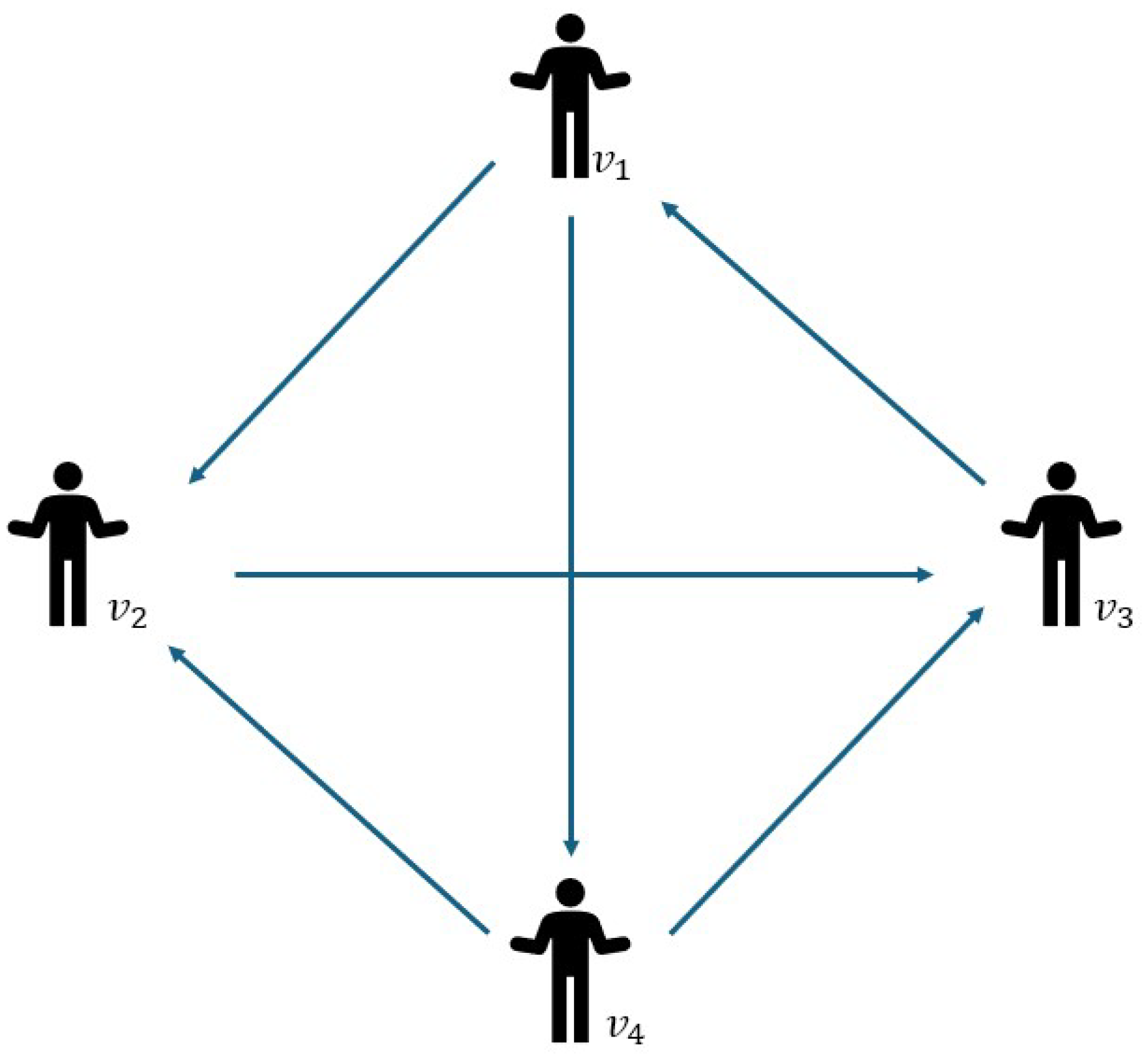
Social networks are often described as directed graphs containing multiple individuals and trust relationships. The nodes represent the individuals in the network, and the connections represent the trust relationships between the individuals. A simple social network is illustrated as Figure 1.

It is difficult for individuals to show complete and full trust in real life. Based on this, Zhang et al. [59] proposed a fuzzy sociometric measure to accurately characterize the level of trust between individuals, with the following basic definition.

Definition 5.

The fuzzy sociometric measure IS =${\left(s_{ij}\right)}_{n\times n}$ on graph $V$ is the relationship with the affiliation function $Us(v_i,v_h)$: $V\times V\to \left[\mathrm{0,1}\right]$ in $V\times V$ and $Us\left(v_i,v_j\right)=s_{ij}$, where $s_{ij}\in \left[\mathrm{0,1}\right]$ denotes the degree of trust that an individual $v_i$ assigns to an individual $v_j$.

It is worth noting that in real life, the fuzzy sociometric measure is not complete. In other words, in authentic social networks, some individuals do not know all the other individuals, so there is no way of directly knowing the corresponding trust degree (e.g., in Figure 1). Therefore, it is crucial to study trust propagation in social networks. In this paper, we will use the trust propagation method based on $t$-norm, provided by Victor et al. [60] to obtain the unknown value of trust in the fuzzy social metric $IS$.

Definition 6.

Let $v_i\to v_{\sigma \left(1\right)}\to v_{\sigma \left(2\right)}\to \dots \to v_{\sigma \left(p\right)}\to v_j$ be a path from $v_i$ to $v_j$ with a path length of $p+1$. In the method proposed by Victor, et al. [60], the value of the degree of trust $s_{ij}$, is evaluated using $t$-norm, which are computed as

$$\begin{gathered} s_{ij}=T\left(s_{i,\sigma \left(1\right)},s_{\sigma \left(1\right),\sigma \left(2\right)},\dots ,s_{\sigma \left(p\right),j}\right) \\ =\frac{2·s_{i,\sigma \left(1\right)}·s_{\sigma \left(p\right),j}·{\prod }_{k=1}^{p-1}{s}_{\sigma \left(k\right),\sigma \left(k+1\right)}}{\left(2-s_{i,\sigma \left(1\right)}\right)·\left(2-s_{\sigma \left(p\right),j}\right)·{\prod }_{k=1}^{p-1}\left(2-s_{\sigma \left(k\right),\sigma \left(k+1\right)}\right)+s_{i,\sigma \left(1\right)}·s_{\sigma \left(p\right),j}·{\prod }_{k=1}^{p-1}{s}_{\sigma \left(k\right),\sigma \left(k+1\right)}}. \end{gathered}$$

(5)

Theoretically, two individuals in a social network may have more than one trust path, so it is crucial to aggregate trust on multiple paths to obtain the total trust. In this paper, the harmonic weighted average operator (HWAO) is taken to aggregate the trust degrees. Assuming that there are $N$ paths from $v_i$ to $v_j$, let $s_{ij}^1,s_{ij}^2,\dots ,s_{ij}^N$ denote the trust values on the N paths. The HWAO operator is used to compute $s_{ij}$ as follows:

$$s_{ij}=\mathrm{H}\mathrm{W}\mathrm{A}\mathrm{O}\left(s_{ij}^1,s_{ij}^2,\dots ,s_{ij}^N\right)=\frac{1}{{\sum }_{k=1}^N\frac{{\rho }_k}{s_{ij}^k}}$$

(6)

In order to determine the weight $\rho ={({\rho }_1,{\rho }_2,\dots ,{\rho }_N)}^T$ in the HWAO operator, this paper will adopt the linguistic quantifier $Q(.)$ proposed by Zadeh [61], which is shown as follows:

$${\rho }_i=Q\left(\frac{i}{N}\right)-Q\left(\frac{i-1}{N}\right),i=\mathrm{1,2},\dots ,N,$$

(7)

and

$$Q\left(c\right)=\left\{\begin{array}{c}\begin{array}{cc}0,& c<a\end{array}\\ \begin{array}{cc}\frac{c-a}{b-a},& a\le c\le b\end{array}\\ \begin{array}{cc}1,& c>b\end{array}\end{array}\right.,$$

(8)

where $a,b,c\in \left[0,1\right]$. Moreover, $\left(a,b\right)$ are $\left(0,1\right),\left(0.3,0.8\right),\left(0,0.5\right)$, and (0.5,1), which denote all, most, at least half, and as many linguistic quantifiers as possible, respectively. Through the above method of trust propagation and trust aggregation in social networks, we can obtain the complete IS =${\left(s_{ij}\right)}_{n\times n}$.

3. Model Construction

This section will firstly introduce the data-driven method combined with trust propagation and aggregation to determine the DMs’ weights. Secondly, we introduce the fair utility level in the CRP, and then construct a variety of uncertainty sets to portray the uncertainty of the unit adjustment cost. Finally, based on the measures of efficiency in reaching consensus and the robust optimization method, we propose a robust consensus model focusing on fairness and efficiency under uncertain costs (EFCM).

3.1. Determination of Weight

In real decision making scenarios, the influence of the decision makers depends not only on the trust in social networks, but also comes from the intrinsic influence of individuals. Differences in the decision makers’ own intrinsic capabilities, such as educational experience, professional skills, and social experience, lead to different decision makers showing differentiated intrinsic influence in group decision making. Therefore, the influence of decision makers in social networks is determined by both intrinsic and extrinsic influences [62]. The influence $w_i$ of decision maker $d_i$ in the social network is calculated as follows:

$$w_i=\alpha {\lambda }_i+\left(1-\alpha \right){NI}_i,$$

(9)

where $\alpha \in \left[\mathrm{0,1}\right]$ is the weight of the intrinsic influence, and ${\lambda }_i\in \left[\mathrm{0,1}\right]$ is the intrinsic influence of decision maker $d_i$. ($1-\mathsf{\alpha }$) is the weight of the extrinsic influence of the social network, and ${NI}_i$ denotes the extrinsic influence of decision maker $d_i$ in the social network. the smaller the value of $\alpha$, the greater the weight of the network influence. Meanwhile, ${NI}_i$ is calculated as

$${NI}_i=\frac{{\sum }_{j\ne i}{s}_{ji}}{{\sum }_i{\sum }_{j\ne i}{s}_{ji}},$$

(10)

where $s_{ji}\in \left[\mathrm{0,1}\right]$ denotes the level of trust that individual $v_j$ has in individual $v_i$, where, if $(v_j,v_i)\in E$, then $s_{ji}$ is given directly by individual $v_j$. Otherwise, $s_{ji}$ is obtained indirectly through trust propagation and aggregation in social networks, as introduced in Section 2.3. It is worth noting that the network influence of an individual in a social network is normalized by the above calculation.

The determination of ${\lambda }_i$ values in existing consensus studies lacks objectivity. To overcome the existing limitations, this section adopts a data-driven approach based on the KDE method to determine the ${\lambda }_i$ value objectively. Assuming that ${\lambda }_k,k=\mathrm{1,2},\dots ,m$ are the observed values of ${\lambda }_i$, the KDE with kernel density function K$(·)$ is defined as

$$\widehat{f}\left({\lambda }_i\right)=\frac{1}{nh}{\sum }_{k=1}^{m}K\left(\frac{{\lambda }_i-{\lambda }_k}{h}\right),$$

(11)

where $\widehat{f}\left({\lambda }_i\right)$ is the estimated density function of the uncertain parameter ${\lambda }_i$ and $m$ is the number of sample points of ${\lambda }_i$. Let the distribution function of variable ${\lambda }_i$ be $F\left({\lambda }_i\right)$, and $P\left({\lambda }_i\le {\lambda }_{\beta }\right)=F\left({\lambda }_{\beta }\right)={\int }_{-\infty }^{{\lambda }_{\beta }}\widehat{f}\left({\lambda }_i\right)d{\lambda }_i=\beta$, where ${\lambda }_{\beta }$ is the quantile that satisfies $P\left({\lambda }_i\le {\lambda }_{\beta }\right)=\beta$. Setting the confidence level of weights according to the quantile λ_β can fully utilize the historical data information. Finally, let ${\lambda }_i={\lambda }_i^{1-{\alpha }_i}=\raisebox{1ex}{$(F_{{\lambda }_i}^{-1}\left(\frac{{\alpha }_i}{2}\right)+F_{{\lambda }_i}^{-1}\left(1-\frac{{\alpha }_i}{2}\right))$}\!\left/ \!\raisebox{-1ex}{$2$}\right.$. The value of ${\lambda }_i$ can be obtained by the above calculation method.

3.2. Fair Utility Level

Definition 7

([48]). Let $o_i$ represent $d_i$’s original opinion, ${\overline{o}}_i$ represents $d_i$’s adjusted opinion and $c_i$ represents $d_i$’s unit adjustment cost. In this paper, $f_i\left(o_i,{\overline{o}}_i\right)=c_i\left|o_i-{\overline{o}}_i\right|$ denotes the compensation (cost) paid by the moderator to $d_i$, then the fairness utility $F^{{(\alpha }_i,{\beta }_i)}\left({\overline{o}}_i,c_i\right)$ of $d_i$ can be expressed as follows:

$$\begin{gathered} F^{{(\alpha }_i,{\beta }_i)}\left({\overline{o}}_i,c_i\right)=f_i\left(o_i,{\overline{o}}_i\right)-\frac{{\alpha }_i{\sum }_{j\ne i}^n\mathit{max}\left\{f_j\left(o_j,{\overline{o}}_j\right)-f_i\left(o_i,{\overline{o}}_i\right),0\right\}}{n-1} \\ -\frac{{\beta }_i{\sum }_{j\ne i}^n\mathit{max}\left\{f_i\left(o_i,{\overline{o}}_i\right)-f_j\left(o_j,{\overline{o}}_j\right),0\right\}}{n-1} \end{gathered}$$

(12)

where  ${\alpha }_i\in \left[\mathrm{0,1}\right]$ represents the jealousy preference coefficient of  $d_i$, and  ${\beta }_i\in \left(-\mathrm{1,1}\right)$ represents the sympathy/pride preference coefficient of  $d_i$.

Different interval values of sympathy/pride preference coefficients have different practical meanings. When ${\beta }_i\in \left(-\mathrm{1,0}\right)$, $d_i$’s fairness utility consists of the compensation, the negative utility generated by the jealousy preference, and the positive utility generated by the pride coefficient [48]. When ${\beta }_i\in \left(\mathrm{0,1}\right)$, the fairness utility consists of the compensation, the negative utility generated by the jealousy preference, and the negative utility generated by the sympathy coefficient [48].

According to fairness theory [39,40], an individual’s sense of fairness depends on social comparisons. In other words, individuals compare the ratio of the incomes received (money, benefits, values, etc.) to the inputs (experience, time, effort, and other exertion of work, etc.) of their work with the ratio of the incomes and inputs of others [39,40]. An individual’s sense of fairness depends on the ratio of fair benefits to actual gains. In this paper, we apply the fair utility level proposed by Du et al. [48] to denote the DM’s sense of fairness.

Definition 8

([48]). If $F^{{(\alpha }_i,{\beta }_i)}\left({\overline{o}}_i,c_i\right)$ denotes the of $d_i$’s fair utility, then the $d_i$’s fair utility level ${FD}^{{(\alpha }_i,{\beta }_i)}\left({\overline{o}}_i,c_i\right)$ can be expressed as follows:

$${FD}^{{(\alpha }_i,{\beta }_i)}\left({\overline{o}}_i,c_i\right)=\left\{\begin{array}{cc}\hfill 0,& F^{{(\alpha }_i,{\beta }_i)}\left({\overline{o}}_i,c_i\right)<0\hfill \\ \hfill \frac{F^{{(\alpha }_i,{\beta }_i)}\left({\overline{o}}_i,c_i\right)}{f_i\left(o_i,{\overline{o}}_i\right)},& 0<F^{{(\alpha }_i,{\beta }_i)}\left({\overline{o}}_i,c_i\right)<f_i\left(o_i,{\overline{o}}_i\right)\hfill \\ \hfill 1,& F^{{(\alpha }_i,{\beta }_i)}\left({\overline{o}}_i,c_i\right)\ge f_i\left(o_i,{\overline{o}}_i\right)\hfill \end{array}.\right.$$

(13)

Clearly, ${FD}^{{(\alpha }_i,{\beta }_i)}\left({\overline{o}}_i,c_i\right)\in \left[\mathrm{0,1}\right]$. $F^{{(\alpha }_i,{\beta }_i)}\left({\overline{o}}_i,c_i\right)<0$ indicates that the $d_i$’s fairness utility is negative, and an individual would consider it grossly unfair, so we define the fair utility level in this condition as 0. If $F^{{(\alpha }_i,{\beta }_i)}\left({\overline{o}}_i,c_i\right)>f_i\left(o_i,{\overline{o}}_i\right)$, then we consider this as excessive fair concern behavior and define the fair utility level as 1 in this case.

Theorem 1.

In GDM, for $f_i\left(o_i,{\overline{o}}_i\right)\ne f_j\left(o_j,{\overline{o}}_j\right)$, $0<F^{{(\alpha }_i,{\beta }_i)}\left({\overline{o}}_i,c_i\right)<f_i\left(o_i,{\overline{o}}_i\right)$, $0\le {\alpha }_i\le 1,{\beta }_i\le {\alpha }_i,-1\le {\beta }_i\le 1;$ when other conditions remain unchanged, the smaller ${\alpha }_i$ is, the larger ${FD}^{{(\alpha }_i,{\beta }_i)}\left({\overline{o}}_i,c_i\right)$ is; and the smaller ${\beta }_i$ is, the larger ${FD}^{{(\alpha }_i,{\beta }_i)}\left({\overline{o}}_i,c_i\right)$ is.

Proof. 

Theorem 1 can be easily proved to hold by the definition of ${FD}^{{(\alpha }_i,{\beta }_i)}\left({\overline{o}}_i,c_i\right)$. □

Theorem 1 shows that the fair utility level is consistent with the fairness preference theory and can effectively depict fair concern behavior in GDM. When the value of a DM’s fair utility level is closer to 1, it means that this DM considers the compensation distribution to be fairer. Therefore, the compensation fairness can be measured by the fair utility level.

From the perspective of the moderator, the moderator expects each DM’s fair utility level t to satisfy a desired value, that is,

$${FD}^{{(\alpha }_i,{\beta }_i)}\left({\overline{o}}_i,c_i\right)\ge \mu ,$$

(14)

where $\mu \in \left[\mathrm{0,1}\right]$ is the group fairness utility level. When ${FD}^{{(\alpha }_i,{\beta }_i)}\left({\overline{o}}_i,c_i\right)\ge \mu$, all the DMs believe that it is fairer and more rational to be compensated for adjusting their opinions, and they are more willing to accept the consensus results, which will stabilize the consensus.

3.3. Uncertainty in Unit Adjustment Cost

Uncertainty factors are widely present in GDM and can impact the consensus results. To reduce the impact of uncertainty factors on the consensus results, this paper will use the robust optimization method to describe the uncertainty of the unit adjustment cost. Assume that the uncertainty of unit adjustment cost is denoted by $Z^c$.

Definition 9.

The uncertainty set $Z^c$ of the individual unit adjustment cost can be expressed as

$$Z^c=\left\{c_i=c_i^o+{\sum }_{l=1}^L{\xi }_l{c}_i^l:\xi \in Z,i\in N=\left\{\mathrm{1,2},\dots ,n\right\}\right\}$$

(15)

where  $c_i^o$ is a fixed value,  $c_i^l$ is a perturbation value of  $c_i$,  ${\xi }_l$ denotes the uncertain parameter vector in a one-dimensional space, and the product of  ${\xi }_l$ and  $c_i^l$ can be interpreted as the uncertainty cost. When the uncertain parameter  $\xi$ does not exist, it means that there is no uncertainty, and  $c_i=c_i^o$ holds. When the uncertain parameters are considered,  $\xi$ depends on different forms of uncertainty sets, and different sets of uncertainties bring a different degree of conservatism to the model. Considering the ease of operation and flexibility, four types of uncertainty sets will be considered in this paper.

3.4. Robust Consensus Model Considering Fairness and Efficiency

Suppose $D=\left\{d_1,\dots ,d_n\right\}$ represents the set of $n$ decision makers involved in group decision making, $o_i(i\in N=\left\{\mathrm{1,2},\dots ,n\right\})$ represents the initial opinion of $d_i$, ${\overline{o}}_i$ represents the adjusted opinion of $d_i$ after a few rounds of adjustments and modifications, and $o^c$ represents the final collective opinion; in other words, the $o^c$ represents the consensus opinion. $c_i$ denotes the unit adjustment cost of $d_i$; in other words, $c_i$ can also denote the cost price that decision maker $d_i$ will pay for the opinion of modifying the program.

In the practical consensus problem, the moderator is concerned not only with the consensus cost but also with the fairness and efficiency in the CRP. From the perspective of consensus stability, the moderator should provide a more relaxed budget to encourage the DMs to fully express and adjust their opinions to reach a fair and efficient consensus. Zhang et al. [14] proposed the adjusted number of DMs, the distance between the original and adjusted preference, and the number of required negotiation rounds to reach consensus as indicators of the consensus reaching efficiency. This paper will use the opinion adjustment distance as the efficiency indicator. When the opinion adjustment distance is farther, the less efficient reaching a consensus is, and conversely, the more efficient it is. Based on this, this paper proposes the Efficiency and Fairness Consensus Model (EFCM) under limited cost, and the specific model form is as follows:

$$\begin{gathered} \mathit{min}{\sum }_{i=1}^n\left|o_i-{\overline{o}}_i\right| \\ s.t.{\sum }_{i=1}^n{c}_i\left|o_i-{\overline{o}}_i\right|\le B_0, \\ 1-\frac{\left|o^c-{\overline{o}}_i\right|}{o^c}\ge \epsilon ,i\in N, \\ {FD}^{{(\alpha }_i,{\beta }_i)}\left({\overline{o}}_i,c_i\right)\ge \mu ,i\in N, \\ {o}^c=F({\overline{o}}_1,{\overline{o}}_2,{\overline{o}}_3,\dots \dots {\overline{o}}_n), \end{gathered}$$

(16)

where $\mu$ represents the group fair utility level, and in this model, $\mu \in \left[\mathrm{0,1}\right]$ will be assigned a definite value. To make it easier to obtain the robust equivalence equation, we reformulate the above model (16) as follows:

EFCM:

$$\begin{gathered} \mathit{min}{\sum }_{i=1}^n\left|o_i-{\overline{o}}_i\right| \\ s.t.c^{T}d\le B_0, \\ 1-\frac{\left|o^c-{\overline{o}}_i\right|}{o^c}\ge \epsilon ,i\in N, \\ {FD}^{{(\alpha }_i,{\beta }_i)}\left({\overline{o}}_i,c_i\right)\ge \mu ,i\in N, \\ {o}^c=F({\overline{o}}_1,{\overline{o}}_2,{\overline{o}}_3,\dots \dots {\overline{o}}_n), \end{gathered}$$

(17)

where $c$ is a matrix consisting of $c_i$ and $c={(c_1,c_2,c_3\dots ,c_n)}^T$, $d$ is a vector of DMs’ opinion adjustment distances, i.e., $d={(\left|o_1-{\overline{o}}_1\right|,\left|o_2-{\overline{o}}_2\right|,\left|o_3-{\overline{o}}_3\right|\dots ,\left|o_n-{\overline{o}}_n\right|)}^T$. T. $B_0$ can be interpreted as the consensus cost budget set by the moderator in the CRP. Furthermore, the constraint $c^{T}d\le B_0$ in model (17) can be reformulated as

$$c^{T}d\le B_0,\forall \left\{c=c_0+c_l{\xi }_l:\xi \in Z\right\}$$

(18)

where $c_0={\left(c_1^o,c_2^o,c_3^o\dots ,c_n^o\right)}^T$, ${\xi }_l={\left({\xi }_1,{\xi }_2,{\xi }_3\dots ,{\xi }_L\right)}^T$, and $c_l={\left(\begin{array}{cc}\begin{array}{cc}{c}_1^1& c_1^2\\ c_2^l& c_2^l\end{array}& \begin{array}{cc}\dots & c_1^L\\ \dots & c_2^L\end{array}\\ \begin{array}{cc}\dots & \dots \\ c_n^1& c_n^2\end{array}& \begin{array}{cc}\dots & \dots \\ \dots & c_n^L\end{array}\end{array}\right)}_{n\times L}$ represents the matrix composed of all the unit-adjusted cost perturbation values.

3.4.1. EFCM Based on Box Set

Firstly, we use the box uncertainty set to describe the unit adjustment cost uncertainty, which is also called the interval set. Without the loss of generality, it can be represented by an infinite paradigm ${‖·‖}_{\infty }$.

Definition 10

([63]). The box set $Z^{Box}$ is defined as

$$Z^{Box}=\left\{\xi \in R^L:{‖{\xi }_l‖}_{\infty }\le \tau \right\}$$

(19)

Theorem 2.

Based on $Z^{Box}$, we can obtain EFCM-B as follows:

EFCM-B:

$$\begin{gathered} \mathit{min}·{\sum }_{i=1}^n\left|o_i-{\overline{o}}_i\right| \\ s.t.{c_0}^{T}d+\tau {‖{c_l}^{T}d‖}_1\le B_0, \\ 1-\frac{\left|o^c-{\overline{o}}_i\right|}{o^c}\ge \epsilon ,i\in N, \\ a+\frac{\tau {‖{c_l}^{T}d‖}_1}{\left(c_i^0\right)\left|o_i-{\overline{o}}_i\right|}\le \left(n-1\right)\left(1-\mu \right),i\in N, \\ {o}^c={\sum }_{i=1}^n(\alpha {\lambda }_i+\left(1-\alpha \right){NI}_i){\overline{o}}_i, \end{gathered}$$

(20)

where  $a=\frac{{\sum }_{j=1}^n\left|\left(c_i^0\right)\left|o_i-{\overline{o}}_i\right|-\left(c_j^0\right)\left|o_j-{\overline{o}}_j\right|\right|}{\left(c_i^0\right)\left|o_i-{\overline{o}}_i\right|}$

Proof. 

According to the definition of $Z^{Box}$, the constraint $c^{T}d\le B_0$ can be transformed into $c^{T}d\le B_0,\forall \left\{c=c_0+c_l{\xi }_l:\xi \in Z\right\}$, which is equivalent to ${\left(c_l{\xi }_l\right)}^{T}d\le B_0-{c_0}^{T}d,\forall \left\{\xi :{‖{\xi }_l‖}_{\infty }\le \tau \right\}$. In other words, $\underset{{‖{\xi }_l‖}_{\infty }\le \tau }{\mathit{max}}{\left(c_l{\xi }_l\right)}^{T}d\le B_0-{c_0}^{T}d$ holds. Since $\underset{{‖{\xi }_l‖}_{\infty }\le \tau }{\mathit{max}}{\left(c_l{\xi }_l\right)}^{T}d=\tau {‖{c_l}^{T}d‖}_1$, the robust equivalence of $c^{T}d\le B_0$ is ${c_0}^{T}d+\tau {‖{c_l}^{T}d‖}_1\le B_0$.

For ${FD}^{{(\alpha }_i,{\beta }_i)}\left({\overline{o}}_i,c_i\right)\ge \mu ,i\in N$, it can be converted to $\frac{{\alpha }_i{\sum }_{j\ne i}^n\max \left\{f_j\left(o_j,{\overline{o}}_j\right)-f_i\left(o_i,{\overline{o}}_i\right),0\right\}}{f_i\left(o_i,{\overline{o}}_i\right)}+\frac{{\beta }_i{\sum }_{j\ne i}^n\max \left\{f_i\left(o_i,{\overline{o}}_i\right)-f_j\left(o_j,{\overline{o}}_j\right),0\right\}}{f_i\left(o_i,{\overline{o}}_i\right)}\le \left(n-1\right)\left(1-\mu \right)$. When ${\alpha }_i\in \left[\mathrm{0,1}\right],{\beta }_i\in \left[-\mathrm{1,1}\right]$, $\max \frac{{\alpha }_i{\sum }_{j\ne i}^n\max \left\{f_j\left(o_j,{\overline{o}}_j\right)-f_i\left(o_i,{\overline{o}}_i\right),0\right\}+{\beta }_i{\sum }_{j\ne i}^n\max \left\{f_i\left(o_i,{\overline{o}}_i\right)-f_j\left(o_j,{\overline{o}}_j\right),0\right\}}{f_i\left(o_i,{\overline{o}}_i\right)}=\frac{{\sum }_{j\ne i}^n\max \left\{f_i\left(o_i,{\overline{o}}_i\right)-f_j\left(o_j,{\overline{o}}_j\right),0\right\}+{\sum }_{j\ne i}^n\max \left\{f_j\left(o_j,{\overline{o}}_j\right)-f_i\left(o_i,{\overline{o}}_i\right),0\right\}}{f_i\left(o_i,{\overline{o}}_i\right)}=\frac{{\sum }_{j=1}^n\left|f_j\left(o_j,{\overline{o}}_j\right)-f_i\left(o_i,{\overline{o}}_i\right)\right|}{f_i\left(o_i,{\overline{o}}_i\right)}$ holds. That is to say that $\frac{{\sum }_{j=1}^n\left|f_j\left(o_j,{\overline{o}}_j\right)-f_i\left(o_i,{\overline{o}}_i\right)\right|}{f_i\left(o_i,{\overline{o}}_i\right)}\le \left(n-1\right)\left(1-\mu \right)$ holds. According to the definition of the uncertainty set $Z^{Box}$, $f_i\left(o_i,{\overline{o}}_i\right)=\left(c_i^o+{\sum }_{l=1}^L{\xi }_i{c}_i^l\right)\left|o_i-{\overline{o}}_i\right|,\frac{{\sum }_{j=1}^n\left|f_j\left(o_j,{\overline{o}}_j\right)-f_i\left(o_i,{\overline{o}}_i\right)\right|}{f_i\left(o_i,{\overline{o}}_i\right)}\le \left(n-1\right)\left(1-\mu \right)$ can be converted into $\frac{{\sum }_{j=1}^n\left|\left(c_i^o+{\sum }_{l=1}^L{\xi }_i{c}_i^l\right)\left|o_i-{\overline{o}}_i\right|-\left(c_j^0+{\sum }_{l=1}^L{\xi }_j{c}_j^l\right)\left|o_j-{\overline{o}}_j\right|\right|}{\left(c_i^0+{\xi }_i{c}_i^l\right)\left|o_i-{\overline{o}}_i\right|}\le \left(n-1\right)\left(1-\mu \right)$.

Since $\underset{{‖{\xi }_l‖}_{\mathrm{\infty }}\le \tau }{\max }\frac{{\sum }_{j=1}^n\left|\left(c_i^o+{\sum }_{l=1}^L{\xi }_i{c}_i^l\right)\left|o_i-{\overline{o}}_i\right|-\left(c_j^0+{\sum }_{l=1}^L{\xi }_j{c}_j^l\right)\left|o_j-{\overline{o}}_j\right|\right|}{\left(c_i^0+{\xi }_i{c}_i^l\right)\left|o_i-{\overline{o}}_i\right|}=\frac{\underset{{‖{\xi }_l‖}_{\mathrm{\infty }}\le \tau }{\max }\left({\sum }_{j=1}^n\left|\left(c_i^0\right)\left|o_i-{\overline{o}}_i\right|-\left(c_j^0+{\sum }_{l=1}^L{\xi }_j{c}_j^l\right)\left|o_j-{\overline{o}}_j\right|\right|\right)}{\left(c_i^0\right)\left|o_i-{\overline{o}}_i\right|}=\frac{\underset{{‖{\xi }_l‖}_{\mathrm{\infty }}\le \tau }{\mathrm{m}\mathrm{a}\mathrm{x}}({\sum }_{j=1}^n\left|\left(c_i^0\right)\left|o_i-{\overline{o}}_i\right|-\left(c_j^0\right)\left|o_j-{\overline{o}}_j\right|+{\sum }_{l=1}^L{\xi }_j{c}_j^l\left|o_j-{\overline{o}}_j\right|\right|)}{\left(c_i^0\right)\left|o_i-{\overline{o}}_i\right|}$ $=\frac{{\sum }_{j=1}^n\left|\left(c_i^0\right)\left|o_i-{\overline{o}}_i\right|-\left(c_j^0\right)\left|o_j-{\overline{o}}_j\right|\right|}{\left(c_i^0\right)\left|o_i-{\overline{o}}_i\right|}+\frac{\underset{{‖{\xi }_l‖}_{\mathrm{\infty }}\le \tau }{\mathit{max}}{\left(c_l{\xi }_l\right)}^{T}d}{\left(c_i^0\right)\left|o_i-{\overline{o}}_i\right|}$, and because $\underset{{‖{\xi }_l‖}_{\mathrm{\infty }}\le \tau }{\mathit{max}}{\left(c_l{\xi }_l\right)}^{T}d=\tau {‖{c_l}^{T}d‖}_1$, $\underset{{‖{\xi }_l‖}_{\mathrm{\infty }}\le \tau }{\max }\frac{{\sum }_{j=1}^n\left|\left(c_i^o+{\sum }_{l=1}^L{\xi }_i{c}_i^l\right)\left|o_i-{\overline{o}}_i\right|-\left(c_j^0+{\sum }_{l=1}^L{\xi }_j{c}_j^l\right)\left|o_j-{\overline{o}}_j\right|\right|}{\left(c_i^0+{\xi }_i{c}_i^l\right)\left|o_i-{\overline{o}}_i\right|}=\frac{{\sum }_{j=1}^n\left|\left(c_i^0\right)\left|o_i-{\overline{o}}_i\right|-\left(c_j^0\right)\left|o_j-{\overline{o}}_j\right|\right|}{\left(c_i^0\right)\left|o_i-{\overline{o}}_i\right|}+\frac{\tau {‖{c_l}^{T}d‖}_1}{\left(c_i^0\right)\left|o_i-{\overline{o}}_i\right|}$, and thus, ${FD}^{{(\alpha }_i,{\beta }_i)}\left({\overline{o}}_i,c_i\right)\ge \mu ,i\in N$ can be transferred to $a+\frac{\tau {‖{c_l}^{T}d‖}_1}{\left(c_i^0\right)\left|o_i-{\overline{o}}_i\right|}\le \left(n-1\right)\left(1-\mu \right)$, where $a=\frac{{\sum }_{j=1}^n\left|\left(c_i^0\right)\left|o_i-{\overline{o}}_i\right|-\left(c_j^0\right)\left|o_j-{\overline{o}}_j\right|\right|}{\left(c_i^0\right)\left|o_i-{\overline{o}}_i\right|}$. □

3.4.2. EFCM Based on Ellipsoid Set

This section will consider the definition of the ellipsoid set. Without the loss of generality, it can be represented by ${‖·‖}_2$.

Definition 11

([63]). The ellipsoid set is defined as

$$Z^{Ellipsoid}=\left\{\xi \in R^L:{‖\xi ‖}_2\le \mathsf{\Omega }\right\}$$

(21)

Theorem 3.

Based on $Z^{Ellipsoid}$, we can obtain EFCM-B as follows:

EFCM-E:

$$\begin{gathered} \mathit{min}{\sum }_{i=1}^n\left|o_i-{\overline{o}}_i\right| \\ s.t.{c_0}^{T}d+\mathsf{\Omega }{‖{c_l}^{T}d‖}_2\le B_0. \\ 1-\frac{\left|o^c-{\overline{o}}_i\right|}{o^c}\ge \epsilon ,i\in N, \\ a+\frac{\mathsf{\Omega }{‖{c_l}^{T}d‖}_2}{\left(c_i^0\right)\left|o_i-{\overline{o}}_i\right|}\le \left(n-1\right)\left(1-\mu \right),i\in N \\ {o}^c={\sum }_{i=1}^n(\alpha {\lambda }_i+\left(1-\alpha \right){NI}_i){\overline{o}}_i, \end{gathered}$$

(22)

where $a=\frac{{\sum }_{j=1}^n\left|\left(c_i^0\right)\left|o_i-{\overline{o}}_i\right|-\left(c_j^0\right)\left|o_j-{\overline{o}}_j\right|\right|}{\left(c_i^0\right)\left|o_i-{\overline{o}}_i\right|}$

Proof. 

According to the definition of the uncertain unit adjustment costs that satisfy the constraints of $Z^{Ellipsoid}$, the constraint $c^{T}d\le B_0$ can be transformed as $c^{T}d\le B_0,\forall \left\{c=c_0+c_l{\xi }_l:\xi \in Z\right\}$, and it is equivalent to ${\left(c_l{\xi }_l\right)}^{T}d\le B_0-{c_0}^{T}d,\forall \left\{\xi :{‖{\xi }_l‖}_{\infty }\le \tau \right\},\forall \left\{\xi :{‖{\xi }_l‖}_2\le \mathsf{\Omega }\right\}$. In other words, $\underset{{‖{\xi }_l‖}_2\le \mathsf{\Omega }}{\max }{\left(c_l{\xi }_l\right)}^{T}d\le B_0-{c_0}^{T}d$ holds. Since $\underset{{‖{\xi }_l‖}_2\le \mathsf{\Omega }}{\max }{\left(c_l{\xi }_l\right)}^{T}d=\mathsf{\Omega }{‖{c_l}^{T}d‖}_2$, the robust equivalence of $c^{T}d\le B_0$ is ${c_0}^{T}d+\mathsf{\Omega }{‖{c_l}^{T}d‖}_2\le B_0$.

Following the derivation in Section 3.4.1, ${FD}^{{(\alpha }_i,{\beta }_i)}\left({\overline{o}}_i,c_i\right)\ge \mu ,i\in N$ can be converted into $\underset{{‖{\xi }_l‖}_2\le \mathsf{\Omega }}{\max }\frac{{\sum }_{j=1}^n\left|\left(c_i^o+{\sum }_{l=1}^L{\xi }_i{c}_i^l\right)\left|o_i-{\overline{o}}_i\right|-\left(c_j^0+{\sum }_{l=1}^L{\xi }_j{c}_j^l\right)\left|o_j-{\overline{o}}_j\right|\right|}{\left(c_i^0+{\xi }_i{c}_i^l\right)\left|o_i-{\overline{o}}_i\right|}\le \left(n-1\right)\left(1-\mu \right)$. Since $\underset{{‖{\xi }_l‖}_2\le \mathsf{\Omega }}{\max }{\left(c_l{\xi }_l\right)}^{T}d=\mathsf{\Omega }{‖{c_l}^{T}d‖}_2$, the equivalent expression for ${FD}^{{(\alpha }_i,{\beta }_i)}\left({\overline{o}}_i,c_i\right)\ge \mu ,i\in N$ is $a+\frac{\mathsf{\Omega }{‖{c_l}^{T}d‖}_2}{\left(c_i^0\right)\left|o_i-{\overline{o}}_i\right|}\le \left(n-1\right)\left(1-\mu \right)$, where $a=\frac{{\sum }_{j=1}^n\left|\left(c_i^0\right)\left|o_i-{\overline{o}}_i\right|-\left(c_j^0\right)\left|o_j-{\overline{o}}_j\right|\right|}{\left(c_i^0\right)\left|o_i-{\overline{o}}_i\right|}$.□

3.4.3. EFCM Based on Box–Ellipsoid Set

Definition 12.

The box–ellipsoid set $Z^{B-E}$ is defined as

$$Z^{B-E}=\left\{\xi \in R^L:{‖\xi ‖}_{\infty }\le 1,{‖\frac{\xi }{\mathsf{\Psi }}‖}_2\le \mathsf{\Omega }\right\}$$

(23)

Remark: here, the uncertainty parameter of the box set is set to a fixed value, i.e.,  $\tau =1$.

Theorem 4.

Based on the form of $Z^{B-E}$, we can obtain EFCM-BE as follows:

EFCM-BE:

$$\begin{gathered} \mathit{min}{\sum }_{i=1}^n\left|o_i-{\overline{o}}_i\right| \\ s.t.{c_0}^{T}d+{‖{\delta }_l‖}_1+\mathsf{\Omega }{‖{{\mathsf{\Psi }}_l\theta }_l‖}_2\le B_0, \\ {\delta }_l+{\theta }_l=-c_l^{\mathrm{T}}d, \\ 1-\frac{\left|o^c-{\overline{o}}_i\right|}{o^c}\ge \epsilon ,i\in N, \\ a+\frac{{‖{\delta }_l‖}_1+\mathsf{\Omega }{‖{\theta }_l‖}_2}{\left(c_i^0\right)\left|o_i-{\overline{o}}_i\right|}\le \left(n-1\right)\left(1-\mu \right),,i\in N \\ {o}^c={\sum }_{i=1}^n(\alpha {\lambda }_i+\left(1-\alpha \right){NI}_i){\overline{o}}_i, \end{gathered}$$

(24)

where  $u_l,v_l$ are the decision variables to be solved, and $a=\frac{{\sum }_{j=1}^n\left|\left(c_i^0\right)\left|o_i-{\overline{o}}_i\right|-\left(c_j^0\right)\left|o_j-{\overline{o}}_j\right|\right|}{\left(c_i^0\right)\left|o_i-{\overline{o}}_i\right|}$.

Proof. 

In general, $Z^{B-E}$ can be expressed in the form of a cone:

$$Z^{B-E}=\left\{\xi \in R^L:\exists \partial \in R^L:R\xi +Q\partial +r\in K\right\}$$

(25)

where $K$ denotes a closed convex cone point and it must be nonempty, and $r$ is an extra vector given in $R^L$. As for $R$ and $Q$, they are given matrices. When the definition is strictly feasible, it is written as

$$Z^{B-E}=\left\{\xi \in R^L:R_1\xi +r_1\in K_1,R_2\xi +r_2\in K_2\right\}.$$

(26)

Thus, we convert $c^{T}d\le B_0$ to

$$\left\{\begin{array}{c}{c_0}^{T}d+r_1{x}_1+r_2{x}_2\le B\\ {c_l}^{T}d+{\left({R_1}^T{x}_1\right)}_l+{\left({R_2}^T{x}_2\right)}_l=0\\ l=1,...L\\ x_1\in K_1^{*},x_2\in K_2^{*}\end{array}\right.,$$

(27)

where

• $R_1\zeta =\left[\xi ;0\right],r_1=\left[0_{L\times 1};1\right]$ and $K_1=\left\{\left(s,t\right)\in R^L\times R:{‖s‖}_{\mathrm{\infty }}\le t\right\}$. Moreover, $K_1=\left\{\left(s,t\right)\in R^L\times R:{‖s‖}_{\mathrm{\infty }}\le t\right\}$ is the dual cone of $K_1^{\mathrm{*}}$ and $K_1^{\mathrm{*}}=\left\{\left(s,t\right)\in R^L\times R:{‖s‖}_1\le t\right\}$.
• In $R_2\zeta =\left[{\sum }^{-1}\xi ;0\right]$, $\sum =diag\{{\mathsf{\Psi }}_1,{\mathsf{\Psi }}_2,{\mathsf{\Psi }}_3,\dots {\mathsf{\Psi }}_L\}$, $r_2=\left[0_{L\times 1};\mathsf{\Omega }\right]$. Since the dual paradigm of the second paradigm is itself, $K_2=K_2^{*}$ holds. In effect, it is a second-order cone.

Then, let $x_1=\left[s_1,t_1\right],x_2=\left[s_2,t_2\right]$; $s_1$ and $s_2$ are one-dimensional while $t_1$ and $t_2$ are $L$-dimensional. In this case, we can rewrite $c^{T}d\le B_0$ as

$$\left\{\begin{array}{c}{c}_0^{T}d+t_1+\mathsf{\Omega }{t}_2\le B\\ {\left(s_1+s_2\right)}_l=-c_l^{T}d\\ l=1,\dots ,L\\ {‖s_1‖}_1\le t_1\\ {‖s_2‖}_2\le t_2\end{array}\right.,$$

(28)

Finally, making $\delta =s_1$, $\theta =s_2$ completes this proof.

Following the above part of the proof, it can be seen that ${FD}^{{(\alpha }_i,{\beta }_i)}\left({\overline{o}}_i,c_i\right)\ge \mu ,i\in N$ can be converted into $\underset{{‖{\xi }_l‖}_2\le \mathsf{\Omega }}{\max }\frac{{\sum }_{j=1}^n\left|\left(c_i^o+{\sum }_{l=1}^L{\xi }_i{c}_i^l\right)\left|o_i-{\overline{o}}_i\right|-\left(c_j^0+{\sum }_{l=1}^L{\xi }_j{c}_j^l\right)\left|o_j-{\overline{o}}_j\right|\right|}{\left(c_i^0+{\xi }_i{c}_i^l\right)\left|o_i-{\overline{o}}_i\right|}\le \left(n-1\right)\left(1-\mu \right)$. According to the above proof, the equivalent expression of ${FD}^{{(\alpha }_i,{\beta }_i)}\left({\overline{o}}_i,c_i\right)\ge \mu ,i\in N$ is equal to $a+\frac{{‖{\delta }_l‖}_1+\mathsf{\Omega }{‖{\theta }_l‖}_2}{\left(c_i^0\right)\left|o_i-{\overline{o}}_i\right|}\le \left(n-1\right)\left(1-\mu \right)$, where $a=\frac{{\sum }_{j=1}^n\left|\left(c_i^0\right)\left|o_i-{\overline{o}}_i\right|-\left(c_j^0\right)\left|o_j-{\overline{o}}_j\right|\right|}{\left(c_i^0\right)\left|o_i-{\overline{o}}_i\right|}$. □

3.4.4. EFCM Based on Box–Polyhedral Set

Definition 13.

Define the box–polyhedron set $Z^{B-P}$ as

$$Z^{B-P}=\left\{\xi \in R^L:{‖\xi ‖}_{\infty }\le 1,{‖\xi ‖}_1\le \mathsf{\Gamma }.\right\}$$

(29)

Remark: here, the uncertainty parameter of the box is set to a fixed value, i.e.,  $\tau =1$.

Theorem 5.

According to the definition of $Z^{B-P}$, we can obtain EFCM-BP as follows:

EFCM-BP:

$$\begin{gathered} \mathit{min}{\sum }_{i=1}^n\left|o_i-{\overline{o}}_i\right| \\ s.t.{c_0}^{T}d+{‖u_l‖}_1+\mathsf{\Gamma }{‖v_l‖}_{\infty }\le B_0, \\ {u}_l+v_l=-c_l^{\mathrm{T}}d \\ 1-\frac{\left|o^c-{\overline{o}}_i\right|}{o^c}\ge \epsilon ,i\in N, \\ a+\frac{{‖u_l‖}_1+\mathsf{\Gamma }{‖v_l‖}_{\infty }}{\left(c_i^0\right)\left|o_i-{\overline{o}}_i\right|}\le \left(n-1\right)\left(1-\mu \right),i\in N, \\ {o}^c={\sum }_{i=1}^n\left(\alpha {\lambda }_i+\left(1-\alpha \right){NI}_i\right){\overline{o}}_i, \end{gathered}$$

(30)

where  $u_l,v_l$ are the decision variables to be solved,  $a=\frac{{\sum }_{j=1}^n\left|\left(c_i^0\right)\left|o_i-{\overline{o}}_i\right|-\left(c_j^0\right)\left|o_j-{\overline{o}}_j\right|\right|}{\left(c_i^0\right)\left|o_i-{\overline{o}}_i\right|}$.

Proof. 

Similarly, $Z^{B-P}$ can be expressed in the form of a cone, and hence, it can be written as

$$Z^{B-P}=\left\{\zeta \in R^L{R}_1\xi +r_1\in K_1,R_2\xi +r_2\in K_2\right\}$$

(31)

We denote $c^{T}d\le B_0$ as a cone:

$$\left\{\begin{array}{c}{c_0}^{T}d+t_1+\mathsf{\Gamma }{t}_2\le B\\ {\left(s_1+s_2\right)}_l=-{c_l}^{T}d\\ {‖s_1‖}_1\le t_1\\ {‖s_2‖}_{\infty }\le t_2\\ l=1,...,L\end{array}I\right.$$

(32)

where

• $R_1\zeta =\left[\xi ;0\right]$, $r_1=\left[0_{L\times 1};1\right]$, and $K_1=\left\{\left[s;t\right]\in R^L\times R:{‖s‖}_{\mathrm{\infty }}\le t\right\}$, where $K_1^{\mathrm{*}}=\left\{\left[s;t\right]\in R^L\times R:{‖s‖}_1\le t\right\}$, and $K_1^{\mathrm{*}}$ is the dual cone of $K_1$.
• $R_2\zeta =\left[\xi ;0\right],r_2=\left[0_{L\times 1}:\mathsf{\Gamma }\right]$ and $K_2=\left\{\left[s;t\right]\in R^L\times R:{‖s‖}_1\le t\right\}=K_1^{\mathrm{*}}$, which implies that $K_2^{\mathrm{*}}$ = $K_1$. This is because 1-paradigm numbers and infinity-paradigm numbers are pairwise-paradigm numbers to each other.

Then, let $x_1=\left[s_1,t_1\right],x_2=\left[s_2,t_2\right]$, where $s_1$, $s_2$ are L-dimensional while $t_1$ and $t_2$ are one-dimensional. Finally, letting $\mu =s_1$ and $\nu =s_2$ completes this proof.

Following the derivation in Section 3.4.3, ${FD}^{{(\alpha }_i,{\beta }_i)}\left({\overline{o}}_i,c_i\right)\ge \mu ,i\in N$ can be converted into $\underset{{‖{\xi }_l‖}_2\le \mathsf{\Omega }}{\max }\frac{{\sum }_{j=1}^n\left|\left(c_i^o+{\sum }_{l=1}^L{\xi }_i{c}_i^l\right)\left|o_i-{\overline{o}}_i\right|-\left(c_j^0+{\sum }_{l=1}^L{\xi }_j{c}_j^l\right)\left|o_j-{\overline{o}}_j\right|\right|}{\left(c_i^0+{\xi }_i{c}_i^l\right)\left|o_i-{\overline{o}}_i\right|}\le \left(n-1\right)\left(1-\mu \right)$. According to the above proof, the equivalent expression of ${FD}^{{(\alpha }_i,{\beta }_i)}\left({\overline{o}}_i,c_i\right)\ge \mu ,i\in N$ is $a+\frac{{‖u_l‖}_1+\mathsf{\Gamma }{‖v_l‖}_{\mathrm{\infty }}}{\left(c_i^0\right)\left|o_i-{\overline{o}}_i\right|}\le \left(n-1\right)\left(1-\mu \right)$, where $a=\frac{{\sum }_{j=1}^n\left|\left(c_i^0\right)\left|o_i-{\overline{o}}_i\right|-\left(c_j^0\right)\left|o_j-{\overline{o}}_j\right|\right|}{\left(c_i^0\right)\left|o_i-{\overline{o}}_i\right|}$. □

4. Simulation

4.1. Numerical Example

This section provides a hypothetical application scenario to illustrate the applicability and rationality of the proposed EFCM.

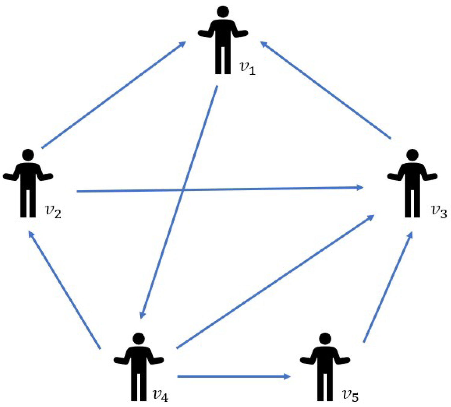
A local government must coordinate some local enterprises to achieve the carbon emission reduction target. Assume that the optimal emission reduction expected by the government is $o^c$, and five heavy polluters $\{v_1,v_2,v_3,v_4,v_5\}$ with considerable economic scales participate in this carbon reduction negotiation; meanwhile, assume that the five enterprises form a network $V=\left\{v_1,v_2,v_3,v_4,v_5\right\},$ as shown in Figure 2.

Let ${\overline{o}}_i$ represent the adjusted emission reduction of $v_i(i\in N=\{\mathrm{1,2},\mathrm{3,4},5\left\}\right)$ and let $c_i$ represent the unit adjustment cost of $v_i$; the initial emission reduction of $v_i$ is $o_i$,$i\in N=\{\mathrm{1,2},\mathrm{3,4},5\}$. Assume that the consensus budget cost of the government is $B_0=25$ (unit: CNY 10,000), and the initial emission reductions of the five enterprises are $o_1=5,o_2=3{,o}_3=7,o_4=4,o_5=6$ (unit: 1000 tons). After consultation and discussion, the consensus level should be no less than 0.5, (i.e., $\epsilon =0.5$). The jealousy preference coefficients of the five enterprises are ${\alpha }_1=0.6,{\alpha }_2=0.7,{\alpha }_3=0.8,{\alpha }_4=0.6,{\alpha }_5=0.5$, the sympathy/pride preference coefficients are ${\beta }_1=0.1,{\beta }_2=0.2{,\beta }_3=0.1,{\beta }_4=0.2,{\beta }_5=0.3$, and the fair utility level of the group is assumed to be 0.6 (i.e., $\mu =0.6$).

It should be noted that when the unit adjustment cost of the enterprises participating in the carbon emission reduction negotiation is recognized as a definite value, it is assumed that $c=c^o={\left\{3,2,4,\mathrm{2.5,3.5}\right\}}^T$ (unit: CNY 10,000/1000 tons). When considering the uncertainty of the unit adjustment cost, to simplify the calculation, we assume that the matrix of the perturbation values of the unit adjustment cost for all the enterprises is $c_l=diag\left(\mathrm{0.1,0.1,0.1,0.1,0.1,0.1}\right)$ (unit: CNY 10,000/1000 tons). Since the uncertainty parameters $\tau ,\mathsf{\Omega },\mathsf{\Gamma }$ have a great influence on the results of the models and the initial setting $\tau =\mathsf{\Omega }=\mathsf{\Gamma }=1$, and to distinguish the box–ellipsoid set from the ellipsoid set, it is assumed that $\mathsf{\Psi }=2$. We use the same uncertainty parameter sizes for the different models. Eventually, all the numerical experiments are performed in Matlab 2018b.

According to the introduction in Section 2.3, assume that the fuzzy sociometric measure $IS=({s_{ij})}_{5\times 5},i,j=\mathrm{1,2},\dots ,5$, which indicates that the value of the degree of trust between the five individuals is

$$IS=\left(\begin{array}{cc}\begin{array}{cc}-& -\\ 0.4& -\end{array}& \begin{array}{ccc}-& 0.1& -\\ 0.7& -& -\end{array}\\ \begin{array}{cc}0.5& -\\ -& 0.9\\ -& -\end{array}& \begin{array}{ccc}-& -& -\\ 0.2& -& 0.6\\ 0.3& -& -\end{array}\end{array}\right).$$

(33)

Firstly, based on the above fuzzy sociometric $IS$, using the trust propagation and trust aggregation methods in Section 2.3, we obtain the complete fuzzy sociometric $S$ as

$$S=\left(\begin{array}{cc}\begin{array}{cc}-& 0.083\\ 0.400& -\end{array}& \begin{array}{ccc}0.047& 0.100& 0.044\\ 0.700& 0.022& 0.008\end{array}\\ \begin{array}{cc}0.500& 0.028\\ 0.143& 0.900\\ 0.111& 0.005\end{array}& \begin{array}{ccc}-& 0.034& 0.015\\ 0.200& -& 0.600\\ 0.300& 0.006& -\end{array}\end{array}\right)$$

(34)

Secondly, according to the above calculation method, the extrinsic influence of the five companies in the social network is ${NI}_1=0.272,{NI}_2=0.239,{NI}_3=0.294,{NI}_4=0.038,{NI}_5=0.157$, respectively. The calculation of the intrinsic influence of the five enterprises is calculated using the data-driven method. Based on the method introduced in Section 3.1, the Gaussian function will be used as the kernel function in this paper. This is mainly because the Gaussian function is continuous and allows for a smoother fit to the data distribution. Moreover, $h$ is the window width, $\widehat{\sigma }$ refers to the standard deviation of the sample, $\widehat{R}$ represents the interquartile range, and the window width can be obtained by $h=1.06·\min \{\widehat{\sigma },(\widehat{R}/1.34)\}·n^{-\left(1/5\right)}$.

Then, 50 groups of $W_{ik},k=\mathrm{1,2},\dots ,50$ such that ${\sum }_{i=1}^5{W}_{ik}=1$, $W_{ik}\in \left[\mathrm{0,1}\right],k=\mathrm{1,2},\dots ,50$ are randomly generated, and the Gaussian KDE results of the four enterprises’ weights are shown in Figure 3. The confidence level of the four weights is set to $1-{\rho }_i=0.75$, and the weights can be obtained as ${\lambda }_1=0.13,{\lambda }_2=0.14$, ${\lambda }_3=0.37,{\lambda }_4=0.18$ and ${\lambda }_5=0.18$, respectively. This part assumes that the intrinsic influence weights are $\alpha =0.5$, and according to the $w_i=\alpha {\lambda }_i+(1-\alpha ){NI}_i$, the social influences of five enterprises are $w_1=0.201$, $w_2=0.19$, $w_3=0.332,w_4=0.109$ and $w_5=0.169$.

When uncertainty about unit adjustment costs is not considered, substituting the above assumed values into the EFCM can obtain the following arithmetic example:

$$\begin{gathered} \mathit{min}(\left|5-{\overline{o}}_1\right|+\left|3-{\overline{o}}_2\right|+\left|7-{\overline{o}}_3\right|+\left|4-{\overline{o}}_4\right|+\left|6-{\overline{o}}_5\right|) \\ s.t.\left(3,2,4,\mathrm{2.5,3.5}\right)d\le 25, \\ 1-\frac{\left|o^c-{\overline{o}}_1\right|}{o^c}\ge 0.5,1-\frac{\left|o^c-{\overline{o}}_2\right|}{o^c}0.5, \\ 1-\frac{\left|o^c-{\overline{o}}_3\right|}{o^c}\ge 0.5,1-\frac{\left|o^c-{\overline{o}}_4\right|}{o^c}\ge 0.5, \\ 1-\frac{\left|o^c-{\overline{o}}_5\right|}{o^c}\ge 0.5, \\ {FD}^{\left(\mathrm{0.6,0.1}\right)}\left({\overline{o}}_1,3\right)\ge 0.6,{FD}^{\left(\mathrm{0.7,0.2}\right)}\left({\overline{o}}_2,2\right)\ge 0.6, \\ {FD}^{\left(\mathrm{0.8,0.1}\right)}\left({\overline{o}}_3,4\right)\ge 0.6,{FD}^{\left(\mathrm{0.6,0.2}\right)}\left({\overline{o}}_4,2.5\right)\ge 0.6, \\ {FD}^{\left(\mathrm{0.5,0.3}\right)}\left({\overline{o}}_5,3.5\right)\ge 0.6, \\ {o}^c=0.201*{\overline{o}}_1+0.19*{\overline{o}}_2+0.332*{\overline{o}}_3+0.109*{\overline{o}}_4+0.169*{\overline{o}}_5, \end{gathered}$$

(35)

where $d={(\left|5-{\overline{o}}_1\right|,\left|3-{\overline{o}}_2\right|,\left|7-{\overline{o}}_3\right|,\left|4-{\overline{o}}_4\right|,\left|6-{\overline{o}}_5\right|)}^T$.

Considering the uncertainty of the unit adjustment cost, the above data can be substituted into EFCM-B, EFCM-E, EFCM-BE, and EFCM-BP, respectively. The solutions of the models EFCM, EFCM-B, EFCM-E, EFCM-BE, and EFCM-BP obtained using Matlab 2018b are shown in

Table 1. Results of the proposed models in this paper.

	$\overline{{\mathit{o}}_1}$	$\overline{{\mathit{o}}_1}$	$\overline{{\mathit{o}}_1}$	$\overline{{\mathit{o}}_1}$	$\overline{{\mathit{o}}_1}$	${\mathbf{o}}^{\mathit{c}}$	Efficiency	$\mathit{B}$
EFCM	1.4298	0.0682	1.3793	1.0318	1.4222	0.8139	10.2433	24.9232
EFCM-B	2.1041	0.6746	0.6621	1.579	2.1057	1.2135	9.0152	16.0081
EFCM-E	4.0709	1.0934	3.3084	3.1719	4.4799	2.4631	7.6259	21.2987
EFCM-BE	1.2355	0.1515	1.5558	1.121	1.3199	0.7095	14.0438	16.9342
EFCM-BP	1.9271	0.275	0.5075	1.3518	1.931	1.1356	11.9539	23.9909

Remark: $B$ is the actual cost of reaching consensus.

and Figure 4.

From Table 1, it is easy to see that when the uncertainty of the unit adjustment cost is not taken into account, the total cost of the EFCM for the five enterprises is 24.9232 (unit: CNY 10,000), which is extremely close to the government’s budget cost (the government sets the cost budget as $B_0=$25 (unit: CNY 10,000). This indicates that the five enterprises will make substantial opinion adjustments in the CRP to maximize the individual compensation benefits and equity of benefits as much as possible, which will delay the collective consensus being reached. When considering the uncertainty in the unit adjustment cost, the total cost for the five enterprises to reach consensus is less than the government budget; in other words, the five enterprises will take a more conservative approach to reach consensus as fast as possible to mitigate the impact of the uncertainty factor on their own compensation benefits. In addition, as the complexity of the uncertainties increases, the efficiency of the five companies in reaching consensus with the government increases, which is accompanied by an increase in the total consensus cost. In other words, in the carbon emission reduction negotiation, the government as a moderator efficiently reaches a consensus by giving more compensation to the five enterprises.

4.2. Comparative Analysis

To reflect the significance of the research in this paper, this section compares the proposed models in this paper with the MACM proposed by Dong et al. [52], and the robust consensus model proposed by Han et al. [64], respectively.

Firstly, by substituting the numerical counterparts in Section 4.1 into the MACM, the following model can be obtained:

$$\begin{gathered} \underset{}{\mathit{min}}\left|5-{\overline{o}}_1\right|+\left|3-{\overline{o}}_2\right|+\left|7-{\overline{o}}_3\right|+\left|4-{\overline{o}}_4\right|+\left|6-{\overline{o}}_5\right| \\ s.t.|{\overline{o}}_1-o^c|\le 0.5, \\ |{\overline{o}}_2-o^c|\le 0.5, \\ |{\overline{o}}_3-o^c|\le 0.5, \\ |{\overline{o}}_4-o^c|\le 0.5, \\ |{\overline{o}}_5-o^c|\le 0.5, \\ {o}^c=0.201*{\overline{o}}_1+0.19*{\overline{o}}_2+0.332*{\overline{o}}_3+0.109*{\overline{o}}_4+0.169*{\overline{o}}_5, \end{gathered}$$

(36)

By using Matlab 2018a, the solution of model (36) is found to be ${\overline{o}}_1=0.957$, ${\overline{o}}_2=0$, ${\overline{o}}_3=0$, ${\overline{o}}_4=0.957$, ${\overline{o}}_4=0.957$, and $o^c=0.4597$ (unit: 1000 tons), and the minimum adjustment distance is found to be 22.1209, and the consensus cost is 71.3628 (unit: CNY 10,000).

Secondly, the robust consensus model (denoted as MCCM-B, MCCM-E) proposed by Han et al. [45] considers uncertainty. The above data are correspondingly substituted into the proposed model, and the model solution results are shown in

Table 2. Results of the model proposed by Han et al. [64].

	$\mathit{F}\mathit{D}\left(\overline{{\mathit{o}}_1}\right)$	$\mathit{F}\mathit{D}\left(\overline{{\mathit{o}}_2}\right)$	$\mathit{F}\mathit{D}\left(\overline{{\mathit{o}}_3}\right)$	$\mathit{F}\mathit{D}\left(\overline{{\mathit{o}}_4}\right)$	$\mathit{F}\mathit{D}\left(\overline{{\mathit{o}}_5}\right)$	$\mathit{B}$
MCCM-B	0.7842	0	0.9461	0.4625	0.8824	77.9413
MCCM-E	0.787	0	0.9465	0.471	0.8834	78.8421

.

Comparing the results of the proposed model, the proposed model in this paper has the following advantages:

(1)

The proposed model in this paper is more efficient and has a lower consensus cost. Take the MACM as an example: The MACM proposed by Dong et al. [52] has a theoretical solution and the total distance of the opinion adjustment is much higher than that of this paper $(22.1209>10.2433)$, in other words, the MACM is less efficient in reaching consensus. Moreover, the consensus budget in the MACM is much higher than the EFCM proposed in this paper $(71.3628>24.9232)$, reflecting that when the government has a sufficient budget, enterprises may adjust their opinions through multiple rounds of negotiation, which increases the overall negotiation cost, and leads to a lower efficiency of reaching consensus.

(2)

The proposed model in this paper is more relevant to the practical GDM scenarios and pays more attention to multiple indicators in the CRP. From the results in Table 2, it is not difficult to find that when there are uncertainties, the fair utility level of enterprise $v_2$ is 0, so enterprise $v_2$ may take non-cooperative measures to hinder the CRP in the actual GDM. In the proposed consensus models (i.e., EFCM-B, EFCM-E, EFCM-BE, EFCM-BP) that consider the uncertain unit adjustment cost, a high fair utility level (i.e., $\mu =0.6$ in Section 4.1) for all the enterprises is ensured, as well as the efficiency of the consensus being reached under a limited cost budget.

4.3. Sensitivity Analysis

In this section, we perform a sensitivity analysis of some parameters in the proposed model to explore the impact of their variations on the model results.

4.3.1. Sensitivity Analysis of Consensus Cost Budget

The proposed consensus model in this paper aims to reach consensus more efficiently and fairly with a limited consensus cost. To explore the effect of different consensus budget costs on the efficiency of reaching consensus, the consensus budget cost $B_0$ is made to vary in the interval $(20,70)$ with a step size of 10, and the other conditions are the same as in Section 4.1. The results of the efficiency (adjustment distance of the opinion) and consensus cost under different consensus cost budgets are shown in

Table 3. Adjustment distance of the opinion under different consensus budgets.

	20	30	40	50	60	70
EFCM	6.6107	9.7484	12.9206	14.3994	15.839	16.2425
EFCM-B	7.4818	10.358	12.9607	15.0529	16.0787	16.9564
EFCM-E	7.946	10.5183	14.9001	16.7752	17.4683	18.3472
EFCM-BE	8.7839	12.0972	17.165	17.4603	17.7757	17.9875
EFCM-BP	13.117	13.7471	16.4441	19.0974	21.5613	22.6664

and

Table 4. Cost of reaching consensus under different consensus budgets.

	20	30	40	50	60	70
EFCM	20.1207	30.0822	40.05	43.4603	48.8724	50.0644
EFCM-B	12.5214	19.6475	27.2221	35.0102	43.9578	35.6324
EFCM-B	17.0516	25.2726	31.8104	43.1147	42.0282	31.6937
EFCM-BE	20.214	30.1506	40.2043	45.6546	39.1401	43.4572
EFCM-BP	20.4165	30.0245	34.3489	48.4952	50.0519	36.6591

.

It is easy to conclude from Figure 4 the following:

(1)

As the consensus budget increases, the efficiency of reaching a consensus decreases (i.e., the adjustment distance of the opinion increases). We argue that enterprises’ pursuits of maximizing their compensation during the negotiation is the reason for this phenomenon. In other words, as the government’s budget increases, enterprises pursue higher compensation gains by constantly revising their opinions, which leads to an overall increase in the adjustment distance of the opinion; in other words, it leads to a decrease in the efficiency of reaching consensus.

(2)

The government should set a reasonable consensus budget. When the consensus budget is low, the budget of the EFCM to reach consensus is equal to the government-set budget. With the increase in the consensus budget, the budget of the EFCM to reach consensus becomes closer to the government-set budget. When the government budget is high, increasing the consensus budget, the efficiency of consensus being reached only increases in a small range, indicating that a consensus budget that is too high cannot significantly improve the efficiency of reaching consensus. Therefore, setting an appropriate consensus budget helps to ensure the efficiency of reaching consensus, and it is recommended that the moderator sets a reasonable consensus budget for actual GDM problems.

4.3.2. Sensitivity Analysis of Consensus Threshold

To explore the impact of different consensus thresholds on the efficiency of reaching consensus, $\epsilon$ is made to vary in the interval [0.1, 1] in steps of 0.1 (

Table 5. Adjustment distance of the opinion under different consensus thresholds.

	0.1	0.2	0.3	0.4	0.5	0.6	0.7	0.8	0.9
EFCM	13.0172	14.143	15.3994	15.5407	15.6651	15.7479	15.9805	16.1608	16.1994
EFCM-B	15.3161	15.5471	15.6458	15.9569	16.2882	16.7567	16.9575	17.1141	17.366
EFCM-E	15.6709	16.4858	17.1722	15.266	16.7752	15.741	16.5135	15.4698	15.5382
EFCM-BE	10.1948	9.1038	11.4718	10.4049	10.8935	8.8979	8.9554	10.5364	9.3254
EFCM-BP	10.8013	10.888	11.474	12.0162	12.0857	12.7641	12.8721	13.3083	13.3464

). Based on the analysis results in Section 4.3.1, the consensus cost budget is set to $B_0=50$ (unit: CNY 10,000) in this section, and the other conditions are the same as those in Section 4.1. Figure 5 illustrates the opinion-adjusted distance for different consensus thresholds.

Figure 5 shows that with the increase in the consensus threshold, the adjustment distance of the opinion in the proposed models shows different trends. In the EFCM, EFCM-B, and EFCM-BP, the values show an overall fluctuating upward trend with the increase in the consensus threshold. Meanwhile, in EFCM-E and EFCM-BE, there is no apparent trend in the opinion-adjusted distance with the increase in the consensus threshold; in other words, the dataset of this study is insensitive to the change in the consensus threshold of the models based on the ellipsoid set and box–ellipsoid set.

4.3.3. Sensitivity Analysis of Perturbation Cost

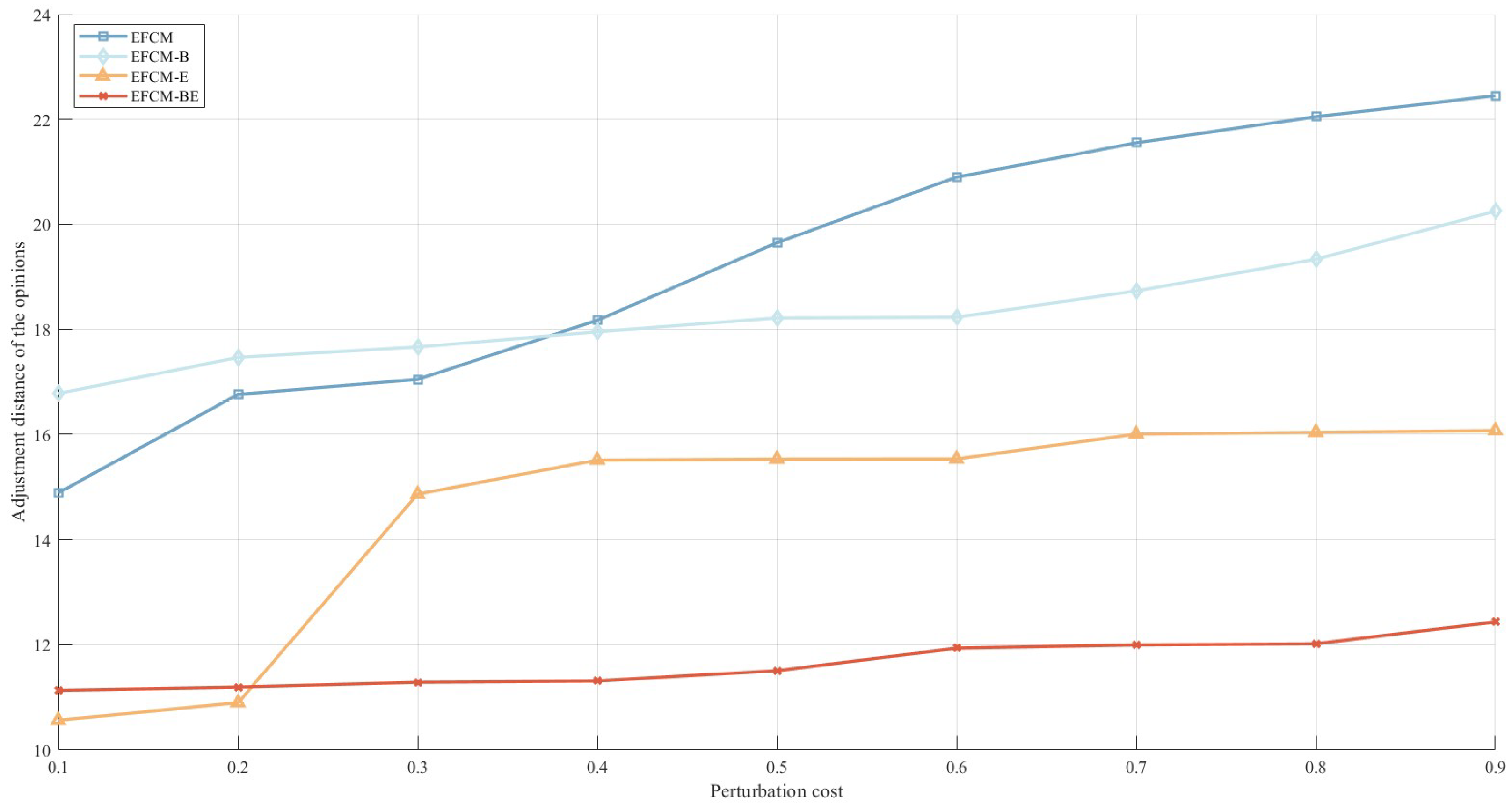
$c_l$ represents the perturbation value of the unit adjustment cost and has an impact on the model’s results. The higher the perturbation value, the higher the chance that the DMs consider the decision risk. In order to explore the effect of different perturbation costs $c_l$ on the efficiency of reaching consensus, let the value in $c_l=diag\left(\mathrm{0.1,0.1,0.1,0.1,0.1,0.1}\right)$ (unit: CNY 10,000/1000 tons) be varied in the interval $\left[0.1,0.9\right]$ with steps of 0.1. Based on the results of the analysis in Section 4.3.1, the consensus cost budget is set to $B_0=50$ (unit: CNY 10,000) in this section, while all other conditions are the same as in Section 4.1;

Table 6. Adjustment distance of the opinion under different perturbation costs.

	0.1	0.2	0.3	0.4	0.5	0.6	0.7	0.8	0.9
EFCM-B	14.8867	16.7567	17.0446	18.1708	19.6465	20.899	21.5537	22.0501	22.4506
EFCM-E	16.7752	17.4627	17.6614	17.9514	18.2154	18.2299	18.7311	19.3342	20.2506
EFCM-BE	10.5635	10.8935	14.862	15.5095	15.5284	15.5327	16.0024	16.0374	16.0714
EFCM-BP	11.1307	11.1929	11.285	11.3102	11.503	11.9331	11.9933	12.0162	12.4327

demonstrates the adjustment distance of the opinion under different perturbation costs.

From Figure 6, it is easy to see that with the increase in the perturbation cost, the adjustment distance of the opinion shows a gradual increase. However, different uncertainty sets show different increasing trends. In EFCM-B, the opinion adjustment distance gradually increases with the increase in the perturbation cost. The increase gradually enlarges, indicating that the box set is more sensitive to perturbations. In EFCM-E, the adjustment distance of the opinion fluctuates less as the perturbation cost increases but shows a slightly increasing trend overall. EFCM-BE has a lower adjustment distance of the opinion at a low perturbation cost, and the increase is more significant when the perturbation cost varies in the interval $[0.3,0.9]$. The model EFCM-BP, with a low adjustment distance at a low perturbation cost, increases more when the perturbation cost varies in the interval [0.6, 0.9]. In other words, when the uncertainty set is a box set, the impact of changes in the perturbation cost is much more significant than that in other uncertainty sets. That is, the box set is the best in improving the model’s robustness.

4.3.4. Sensitivity Analysis of Uncertainty Parameter Level

The uncertainty parameters determine the size of the uncertainty set. Different shapes of uncertainty sets contain different types of uncertainty parameters. To explore the effect of different uncertainty parameter levels $\tau$, $\mathsf{\Omega },\mathsf{\Gamma }$ on the efficiency of reaching consensus, the values in $\tau$, $\mathsf{\Omega },\mathsf{\Gamma }$ are made to vary in the interval $[1,5]$ in steps of 1. Based on the analysis results in Section 4.3.1, this section sets the consensus cost budget to $B_0=50$ (unit: CNY 10,000), while other conditions the same as in Section 4.1.

Table 7. Adjustment distance of the opinion under uncertainty parameter levels.

	1	2	3	4	5
EFCM-B	15.5471	17.1542	18.6913	20.1231	20.7203
EFCM-E	16.7752	17.0197	17.7207	18.6869	19.4116
EFCM-BE	13.0068	10.8935	9.6779	9.4527	9.2381
EFCM-BP	16.5269	11.6638	11.5449	11.4584	11.4059

demonstrates the opinion-adjusted distances at the uncertainty parameter levels.

Figure 7 shows the effect of the variation in the uncertainty parameters on the consensus efficiency. It is not difficult to find that the effect of the variation in the uncertainty parameters on the consensus efficiency is different depending on the type of uncertainty set. Specifically, when the uncertainty set is a box set and an ellipsoid set, the efficiency of reaching consensus decreases with the increase in the uncertain parameter level; in other words, the adjustment distance of the opinion becomes larger with the increase in the uncertain parameter level, and the box set influences the effect slightly more than the ellipsoid set. On the contrary, when the uncertainty set is a box–ellipsoid set and a box–polyhedron set, the efficiency of reaching consensus increases as the uncertainty parameter level increases, and the box–polyhedron set influences the effect on the efficiency of consensus slightly more than the box–ellipsoid set.

4.3.5. Sensitivity Analysis of Group Fair Utility Level

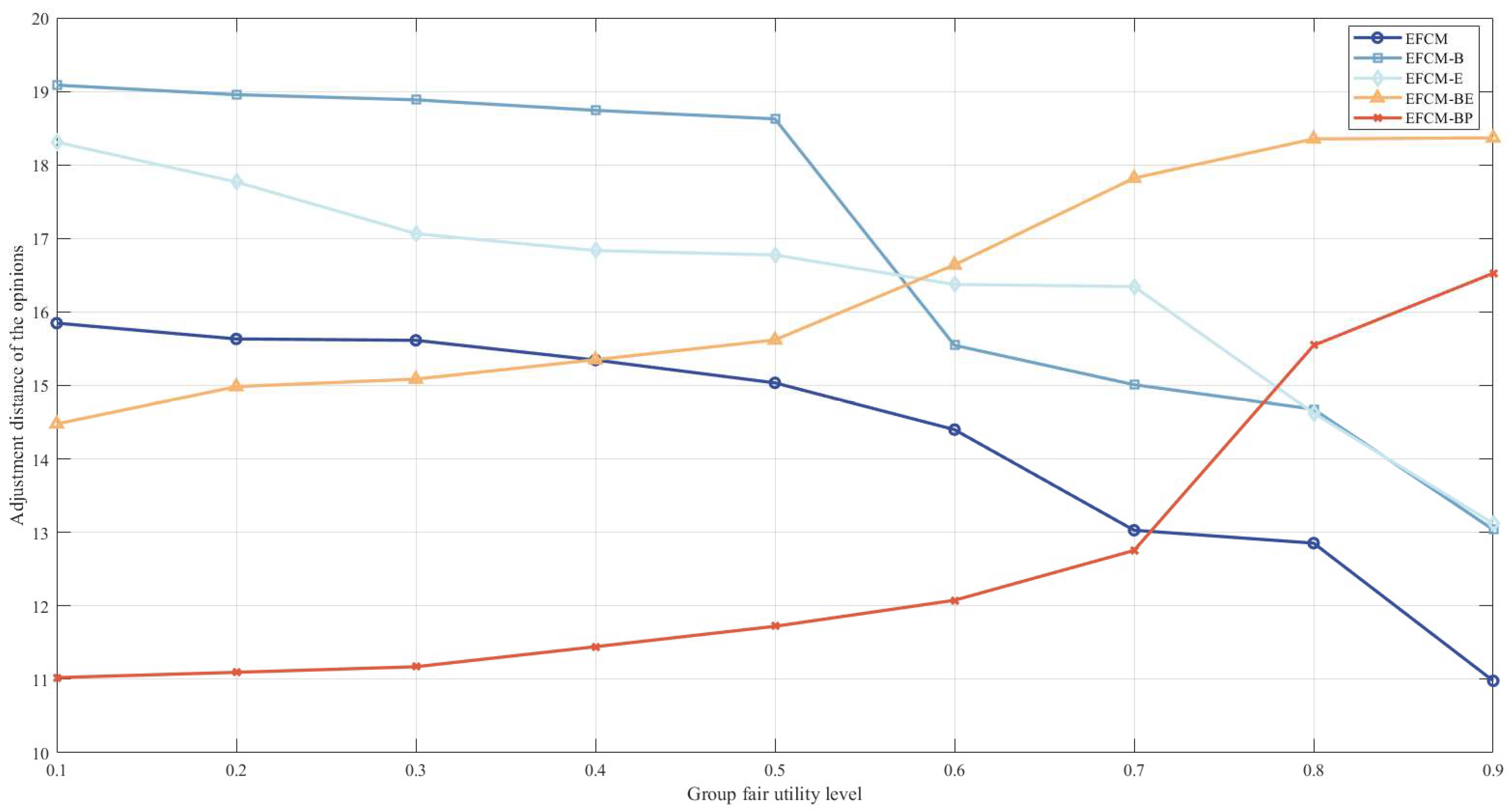
To explore the impact of different group fair utility levels $\mu$ on the efficiency of reaching consensus, the value of $\mu$ is made to vary in the interval [0.1, 0.9] in steps of 0.1 (

Table 8. Adjustment distance of the opinion under different group fair utility levels.

	0.1	0.2	0.3	0.4	0.5	0.6	0.7	0.8	0.9
EFCM	15.8481	15.6333	15.6144	15.3462	15.0359	14.3994	13.0294	12.854	10.9792
EFCM-B	19.0852	18.9557	18.8851	18.7421	18.626	15.5471	15.0112	14.6771	13.0382
EFCM-E	18.3098	17.7684	17.0651	16.8359	16.7752	16.3747	16.3454	14.6241	13.1201
EFCM-BE	14.4774	14.9848	15.0872	15.3507	15.6197	16.6413	17.8202	18.3536	18.3674
EFCM-BP	11.0231	11.0946	11.1709	11.4438	11.7217	12.076	12.7541	15.5456	16.5269

). Based on the analysis results in Section 4.3.1, this section sets the consensus cost budget to $B_0=50$ (unit: CNY 10,000), and other conditions are the same as in Section 4.1. Figure 8 demonstrates the adjustment distance of the opinion under different group fair utility levels.

It is easy to see that the change in the group fair utility level leads to different trends in the adjustment distance of the opinion. Specifically, in the EFCM, EFCM-B, and EFCM-E, the adjustment distance of the opinion decreases with the increase in the group fair utility level. In contrast, in EFCM-BE and EFCM-BP, the adjustment distance of the opinion increases with the increase in the group fair utility level. In addition, as the group fair utility level increases, the EFCM has the largest change in the efficiency of reaching consensus and the EFCBP displays the smallest change in the efficiency of reaching consensus, indicating that the results of the consensus models that consider uncertainty are more conservative.

4.3.6. Sensitivity Analysis of Fair Concern Behavior

In this section, we will analyze the impact of corporate fair attention behaviors (jealousy preference, sympathy preference, pride preference) on the consensus reaching efficiency.

Firstly, we will analyze the change in the consensus reaching efficiency under different jealousy preference coefficients. Since enterprise $v_3$ has the largest weight, this section lets the jealousy preference coefficient (${\alpha }_3$) of enterprise $v_3$ vary at [0.1, 0.9] in steps of 0.1. To simplify the analysis, it is assumed that ${\beta }_1={\beta }_2={\beta }_3={\beta }_4={\beta }_5=0$. Two cases are considered: case 1: ${\alpha }_1={\alpha }_2={\alpha }_4={\alpha }_5=0$, and case 2: ${\alpha }_1={\alpha }_2={\alpha }_4={\alpha }_5=1$. The results are summarized in

Table 9. Adjustment distance of the opinion under different jealousy preference coefficients in case 1.

	0	0.1	0.2	0.3	0.4	0.5	0.6	0.7	0.8	0.9	1
EFCM	15.0828	15.0836	15.0824	15.0826	15.0832	15.0833	15.0805	15.0797	15.0804	15.0798	15.5921
EFCM-B	18.9297	18.9247	19.2734	19.2315	18.7989	18.7923	18.7793	18.7543	18.7513	18.7393	18.7325
EFCM-E	18.0057	18.3617	18.4923	19.1581	17.577	18.6388	18.6092	18.6166	18.6382	18.5911	18.6464
EFCM-BE	13.764	13.2629	14.0104	14.1305	14.1447	13.9202	13.8389	13.3599	13.3706	14.1217	14.2109
EFCM-BP	10.9244	10.9187	10.9137	10.9049	10.8953	10.8857	10.876	10.8662	10.8565	10.8469	10.8376

and

Table 10. Adjustment distance of the opinion under different jealousy preference coefficients in case 2.

	0	0.1	0.2	0.3	0.4	0.5	0.6	0.7	0.8	0.9	1
EFCM	12.7218	12.851	12.912	12.929	12.965	13.029	13.166	13.469	13.706	15.239	15.291
EFCM-B	13.1835	13.186	13.188	13.192	13.194	13.196	13.197	13.200	15.040	16.143	16.446
EFCM-E	13.4631	13.469	13.834	14.042	14.629	16.407	16.856	16.902	16.909	17.172	17.334
EFCM-BE	16.2986	16.344	16.833	17.112	17.622	17.816	17.972	18.250	18.316	18.398	18.446
EFCM-BP	11.4241	11.92	12.076	12.082	12.168	12.30	12.53	12.567	12.597	13.782	15.146

.

It is easy to conclude from Figure 9 and Figure 10 the following:

(1)

The jealousy preference of all the DMs has a stronger impact on the efficiency of reaching consensus in the CRP. When the other DMs do not have a jealous preference (i.e., case 1), the adjustment distance of the opinion fluctuates in a small interval as the jealous preference coefficient increases, indicating that the jealous preference behavior of a single DM cannot significantly affect the group’s efficiency of reaching consensus. When other DMs have a full jealousy preference (i.e., case 2), as the jealousy preference coefficient increases, the adjustment distance of the opinion increases, indicating that all the DMs exhibit jealousy preference behavior, which significantly affects the efficiency of reaching consensus.

(2)

Secondly, comparing Table 9 and Table 10, whether all the DMs exhibit jealousy preference behavior or not has different effects on the efficiency of reaching consensus. Specifically, in the EFCM, EFCM-B, and EFCM-E, when all the DMs exhibit jealous preference behavior, it increases the adjustment distance of the opinion compared to when a single DM exhibits jealous preference behavior. In other words, when all the DMs exhibit jealous preference behavior, reaching consensus will be less efficient. Conversely, in EFCM-BE and EFCM-BP, when all the DMs exhibit jealousy preference behavior, it leads to a decrease in the adjustment distance of the opinion compared to when a single DM exhibits jealous preference behavior.

Next, we will analyze the effect on consensus reaching efficiency under different sympathetic preference coefficients. To simplify the analysis, it is assumed that ${\alpha }_1={\alpha }_2={\alpha }_3={\alpha }_4={\alpha }_5=0$. Similarly, two cases are considered—case 1: ${\beta }_1={\beta }_2={\beta }_4={\beta }_5=0$, and case 2: ${\beta }_1={\beta }_2={\beta }_4={\beta }_5=1$. This section allows the sympathetic preference coefficient ${\beta }_3$ of enterprise $v_3$ to vary at [0.1, 1] in steps of 0.1, and the results are summarized in

Table 11. Adjustment distance of the opinion under different sympathy preference coefficients in case 1.

	0	0.1	0.2	0.3	0.4	0.5	0.6	0.7	0.8	0.9	1
EFCM	15.083	15.088	15.100	15.079	15.083	15.083	15.410	15.707	16.611	16.202	17.014
EFCM-B	18.930	18.913	18.910	18.665	18.757	18.754	18.423	19.696	19.668	19.875	20.558
EFCM-E	18.006	18.186	18.279	17.868	18.621	18.331	17.255	19.354	19.898	17.799	18.834
EFCM-BE	16.759	15.961	12.828	17.077	17.295	13.599	13.760	13.916	12.086	13.550	16.587
EFCM-BP	10.924	10.927	10.922	10.911	10.894	10.876	11.096	11.549	12.498	12.302	11.741

and

Table 12. Adjustment distance of the opinion under different sympathy preference coefficients in case 2.

	0	0.1	0.2	0.3	0.4	0.5	0.6	0.7	0.8	0.9	1
EFCM	15.965	15.140	15.806	15.961	15.933	15.076	15.982	15.708	15.897	16.931	16.215
EFCM-B	19.250	18.954	19.177	18.835	18.914	18.992	19.134	19.640	19.782	19.849	20.014
EFCM-E	16.941	18.815	18.969	18.914	18.702	18.839	18.923	16.698	19.557	18.026	21.330
EFCM-BE	17.527	17.689	16.500	14.830	17.819	19.078	17.941	18.867	21.041	20.762	15.708
EFCM-BP	10.852	10.818	10.885	10.868	10.858	10.868	11.419	11.536	13.329	12.177	14.038

.

Comparing Figure 11 and Figure 12, it is easy to see that the sympathetic preference behavior of all the DMs cannot significantly affect the efficiency of reaching consensus. Specifically, whether a single DM exhibits sympathetic preference behavior, or all the DMs exhibit sympathetic preference behavior, the adjustment distance of the opinion fluctuates within a small range without a significant trend; in other words, the DMs’ sympathetic preference behaviors cannot significantly affect the efficiency of reaching consensus.

Finally, we will analyze the effect of different pride preference coefficients on the efficiency of reaching consensus. To simplify the analysis, it is assumed that ${\alpha }_1={\alpha }_2={\alpha }_3={\alpha }_4={\alpha }_5=0$. Similarly, two cases are considered—case 1: ${\beta }_1={\beta }_2={\beta }_4={\beta }_5=0$, and case 2: ${\beta }_1={\beta }_2={\beta }_4={\beta }_5=-1$. This section allows the pride preference coefficient ${\beta }_3$ of enterprise $v_3$ to vary at [−1, 0] in steps of 0.1, and the results are summarized in

Table 13. Adjustment distance of the opinion under different pride preference coefficients in case 1.

	−1	−0.9	−0.8	−0.7	−0.6	−0.5	−0.4	−0.3	−0.2	−0.1	0
EFCM	15.127	15.119	15.747	15.763	15.068	15.104	15.103	15.101	15.094	15.091	15.083
EFCM-B	18.822	18.809	18.796	18.769	18.738	18.747	18.625	18.620	19.158	18.930	18.715
EFCM-E	18.682	18.683	18.689	18.612	18.614	18.588	18.551	18.473	18.553	19.091	18.006
EFCM-BE	10.158	10.462	10.036	10.393	10.393	10.289	10.792	10.87	10.951	10.759	10.345
EFCM-BP	10.809	10.712	10.697	10.682	10.666	10.659	10.604	10.591	10.588	10.597	10.924

and

Table 14. Adjustment distance of the opinion under different pride preference coefficients in case 2.

	−1	−0.9	−0.8	−0.7	−0.6	−0.5	−0.4	−0.3	−0.2	−0.1	0
EFCM	15.497	15.871	15.858	16.078	15.823	15.733	15.493	15.837	15.423	15.387	15.828
EFCM-B	18.676	18.916	18.702	18.676	18.713	18.721	18.721	18.730	18.453	18.948	18.850
EFCM-E	18.861	18.408	18.631	18.883	18.411	18.534	18.616	18.763	18.696	18.985	18.590
EFCM-BE	10.296	2.938	2.945	4.524	4.253	2.037	1.996	11.463	14.708	7.852	8.236
EFCM-BP	10.613	10.611	10.614	10.630	10.658	10.495	10.527	10.569	10.665	10.799	10.627

.

Comparing Figure 13 and Figure 14, it is easy to see that in GDM, the pride preference behavior of all the DMs cannot significantly affect the efficiency of reaching consensus. Specifically, whether a single DM exhibits pride preference behavior, or all the DMs exhibit pride preference behavior, the adjustment distance of the opinion fluctuates within a small range, with no obvious trend; in other words, the DMs′ pride preference behaviors cannot significantly affect the efficiency of reaching consensus either.

5. Conclusions

This paper studies robust consensus modeling under uncertain costs, focusing on the fairness and efficiency of reaching consensus. Firstly, this paper determines the DMs’ weights by combining the data-driven method with the social network trust propagation method in the CRP. Secondly, this paper applies the group fair utility level to measure the fairness of consensus and uses the adjustment distance of the opinion to measure the efficiency of reaching consensus. Moreover, this paper constructs four types of uncertainty sets to describe the uncertainty of the unit adjustment cost and proposes robust consensus models focusing on fairness and efficiency under uncertain costs. Finally, this paper proves the rationality of the proposed model by applying them to the carbon emission reduction negotiation between the government and enterprises. Compared with the current consensus research, the main innovations of this paper are shown as follows:

(1)

This paper proposes robust group consensus models focusing on fairness and efficiency, studies how to reach consensus efficiently and fairly under uncertain costs and enriches the theoretical system of group consensus research.

(2)

This paper utilizes a data-driven approach combined with the trust transfer method in social networks to jointly determine the weights of the decision makers. Compared with the single method of determining DMs’ weights based on the subjective experience of moderators or the trust degree in social networks in existing studies, the method of determining weights by combining data-driven methods and trust transfer in social networks adopted in this paper is more scientific and objective.

In addition, a sensitivity analysis reveals the characteristics of some of the parameters in the model, leading to the following conclusions:

(1)

Comparing the MACM proposed by Dong et al. [52] and the robust consensus models proposed by Han et al. [64], the proposed models in this paper have a higher efficiency of reaching consensus and a lower consensus cost. In addition, compared with the above studies, the proposed models in this paper are more relevant to GDM problems and pay more attention to multiple metrics in the CRP.

(2)

There are differences in the effects of the perturbation cost and uncertainty parameter level on the efficiency of reaching consensus. Specifically, with the increase in the perturbation cost, the adjustment distance of the opinion shows a trend of gradual increase. For the uncertain parameter level, when the uncertainty set is a box set and ellipsoid set, with the increase in the uncertain parameter level, the efficiency of reaching consensus decreases (the adjustment distance of the opinion increases), and when the uncertainty set is a box–ellipsoid set and a box–polyhedron set, with the increase in the uncertainty parameter level, the efficiency of reaching consensus increases (the opinion adjustment distance becomes decreases). Therefore, when faced with GDM of varying complexity, the moderator should choose different uncertainty sets with an appropriate uncertainty parameter level to accurately characterize the uncertainty cost.

(3)

Taking the negotiation between the government and enterprises on carbon emission reduction as an example, the government should pay full attention to the fair concern behavior shown by enterprises in the CRP, and mainly avoid DMs’ unreasonable jealousy preference behavior. Furthermore, the government can formulate a reasonable consensus cost budget to ensure a reasonable group fair utility level and the efficiency of reaching consensus.

There are also limitations of this paper and some feasible future research directions:

(1)

Only one consensus efficiency measure is used in this paper to construct the consensus model. So, different consensus efficiency measures could be flexibly adopted for future consensus scenarios.

(2)

The social network structure considered in this paper is static. However, the connections between individuals may change dynamically in real SNGDM, and the individual weights evolve dynamically as a result. So, it could be possible to study consensus based on the dynamic social network structure in the future.

References

- Baucells, M.; Sarin, R.K. Group decisions with multiple criteria. Manag. Sci. 2003, 49, 1105–1118. [Google Scholar] [CrossRef]
- Hochbaum, D.S.; Levin, A. Methodologies and algorithms for group-rankings decision. Manag. Sci. 2006, 52, 1394–1408. [Google Scholar] [CrossRef]
- Wallenius, J.; Dyer, J.S.; Fishburn, P.C.; Steuer, R.E.; Zionts, S.; Deb, K. Multiple criteria decision making, multiattribute utility theory: Recent accomplishments and what lies ahead. Manag. Sci. 2008, 54, 1336–1349. [Google Scholar] [CrossRef]
- Zhang, H.; Wang, F.; Dong, Q.; Gong, Z.; Wu, J.; Wu, Z.; Xu, Y.; Zhang, Z.; Dong, Y. Consensus in Group Decision Making: Research Progress and Prospect. J. UESTC 2021, 23, 26–37. [Google Scholar]
- Wu, J.; Chiclana, F.; Herrera-Viedma, E. Trust based consensus model for social network in an incomplete linguistic information context. Appl. Soft Comput. 2015, 35, 827–839. [Google Scholar] [CrossRef]
- Recio-García, J.A.; Quijano, L.; Díaz-Agudo, B. Including social factors in an argumentative model for group decision support systems. Decis. Support Syst. 2013, 56, 48–55. [Google Scholar] [CrossRef]
- Herrera-Viedma, E.; Cabrerizo, F.J.; Chiclana, F.; Wu, J.; Cobo, M.J.; Konstantin, S. Consensus in group decision making and social networks. Stud. Inform. Control 2017, 26, 259–268. [Google Scholar] [CrossRef]
- Dong, Y.; Zha, Q.; Zhang, H.; Kou, G.; Fujita, H.; Chiclana, F.; Herrera-Viedma, E. Consensus reaching in social network group decision making: Research paradigms and challenges. Knowl.-Based Syst. 2018, 162, 3–13. [Google Scholar] [CrossRef]
- Capuano, N.; Chiclana, F.; Fujita, H.; Herrera-Viedma, E.; Loia, V. Fuzzy group decision making with incomplete information guided by social influence. IEEE Trans. Fuzzy Syst. 2017, 26, 1704–1718. [Google Scholar] [CrossRef]
- Herrera-Viedma, E.; Alonso, S.; Chiclana, F.; Herrera, F. A consensus model for group decision making with incomplete fuzzy preference relations. IEEE Trans. Fuzzy Syst. 2007, 15, 863–877. [Google Scholar] [CrossRef]
- Herrera-Viedma, E.; Herrera, F.; Chiclana, F. A consensus model for multiperson decision making with different preference structures. IEEE Trans. Syst. Man Cybern. Part A Syst. Hum. 2002, 32, 394–402. [Google Scholar] [CrossRef]
- Ben-Arieh, D.; Easton, T.; Evans, B. Minimum cost consensus with quadratic cost functions. IEEE Trans. Syst. Man Cybern. Part A Syst. Hum. 2008, 39, 210–217. [Google Scholar] [CrossRef]
- Herrera, F.; Herrera-Viedma, E.; Verdegay, J.L. A rational consensus model in group decision making using linguistic assessments. Fuzzy Sets Syst. 1997, 88, 31–49. [Google Scholar] [CrossRef]
- Zhang, H.; Dong, Y.; Chiclana, F.; Yu, S. Consensus efficiency in group decision making: A comprehensive comparative study and its optimal design. Eur. J. Oper. Res. 2019, 275, 580–598. [Google Scholar] [CrossRef]
- Zhang, H.; Kou, G.; Peng, Y. Soft consensus cost models for group decision making and economic interpretations. Eur. J. Oper. Res. 2019, 277, 964–980. [Google Scholar] [CrossRef]
- Gong, Z.; Zhang, H.; Forrest, J.; Li, L.; Xu, X. Two consensus models based on the minimum cost and maximum return regarding either all individuals or one individual. Eur. J. Oper. Res. 2015, 240, 183–192. [Google Scholar] [CrossRef]
- Liu, J.; Chan, F.T.; Li, Y.; Zhang, Y.; Deng, Y. A new optimal consensus method with minimum cost in fuzzy group decision. Knowl.-Based Syst. 2012, 35, 357–360. [Google Scholar] [CrossRef]
- Gong, Z.; Xu, X.; Lu, F.; Li, L.; Xu, C. On consensus models with utility preferences and limited budget. Appl. Soft Comput. 2015, 35, 840–849. [Google Scholar] [CrossRef]
- Gong, Z.; Xu, X.; Zhang, H.; Ozturk, U.A.; Herrera-Viedma, E.; Xu, C. The consensus models with interval preference opinions and their economic interpretation. Omega 2015, 55, 81–90. [Google Scholar] [CrossRef]
- Gong, Z.; Guo, W.; Herrera-Viedma, E.; Gong, Z.; Wei, G. Consistency and consensus modeling of linear uncertain preference relations. Eur. J. Oper. Res. 2020, 283, 290–307. [Google Scholar] [CrossRef]
- Tan, X.; Gong, Z.; Chiclana, F.; Zhang, N. Consensus modeling with cost chance constraint under uncertainty opinions. Appl. Soft Comput. 2018, 67, 721–727. [Google Scholar] [CrossRef]
- Ji, Y.; Li, H.; Zhang, H. Risk-averse two-stage stochastic minimum cost consensus models with asymmetric adjustment cost. Group Decis. Negot. 2022, 31, 261–291. [Google Scholar] [CrossRef] [PubMed]
- Wei, J.; Qu, S.; Wang, Q.; Luan, D.; Zhao, X. The novel data-driven robust maximum expert mixed integer consensus models under multirole’s opinions uncertainty by considering noncooperators. IEEE Trans. Comput. Soc. Syst. 2022, 10, 3454–3470. [Google Scholar] [CrossRef]
- Gou, X.; Xu, Z.; Liao, H. Group decision making with compatibility measures of hesitant fuzzy linguistic preference relations. Soft Comput. 2019, 23, 1511–1527. [Google Scholar] [CrossRef]
- Li, H.; Ji, Y.; Gong, Z.; Qu, S. Two-stage stochastic minimum cost consensus models with asymmetric adjustment costs. Inf. Fusion 2021, 71, 77–96. [Google Scholar] [CrossRef]
- Ji, Y.; Li, Y.; Wijekoon, C. Robust two-stage minimum asymmetric cost consensus models under uncertainty circumstances. Inf. Sci. 2024, 663, 120279. [Google Scholar] [CrossRef]
- Qu, S.; Han, Y.; Wu, Z.; Raza, H. Consensus modeling with asymmetric cost based on data-driven robust optimization. Group Decis. Negot. 2021, 30, 1395–1432. [Google Scholar] [CrossRef]
- Cabrerizo, F.J.; Morente-Molinera, J.A.; Pedrycz, W.; Taghavi, A.; Herrera-Viedma, E. Granulating linguistic information in decision making under consensus and consistency. Expert Syst. Appl. 2018, 99, 83–92. [Google Scholar] [CrossRef]
- Pérez, I.J.; Cabrerizo, F.J.; Alonso, S.; Herrera-Viedma, E. A new consensus model for group decision making problems with non-homogeneous experts. IEEE Trans. Syst. Man Cybern. Syst. 2013, 44, 494–498. [Google Scholar] [CrossRef]
- Wu, Y.; Dong, Y.; Qin, J.; Pedrycz, W. Flexible linguistic expressions and consensus reaching with accurate constraints in group decision-making. IEEE Trans. Cybern. 2019, 50, 2488–2501. [Google Scholar] [CrossRef]
- Alonso, S.; Pérez, I.J.; Cabrerizo, F.J.; Herrera-Viedma, E. A linguistic consensus model for web 2.0 communities. Appl. Soft Comput. 2013, 13, 149–157. [Google Scholar] [CrossRef]
- Cheng, D.; Cheng, F.; Zhou, Z.; Wu, Y. Reaching a minimum adjustment consensus in social network group decision-making. Inf. Fusion 2020, 59, 30–43. [Google Scholar] [CrossRef]
- Liang, Q.; Liao, X.; Liu, J. A social ties-based approach for group decision-making problems with incomplete additive preference relations. Knowl.-Based Syst. 2017, 119, 68–86. [Google Scholar] [CrossRef]
- Wu, J.; Chiclana, F.; Fujita, H.; Herrera-Viedma, E. A visual interaction consensus model for social network group decision making with trust propagation. Knowl.-Based Syst. 2017, 122, 39–50. [Google Scholar] [CrossRef]
- Wu, T.; Zhang, K.; Liu, X.; Cao, C. A two-stage social trust network partition model for large-scale group decision-making problems. Knowl.-Based Syst. 2019, 163, 632–643. [Google Scholar] [CrossRef]
- Ding, Z.; Chen, X.; Dong, Y.; Herrera, F. Consensus reaching in social network DeGroot Model: The roles of the Self-confidence and node degree. Inf. Sci. 2019, 486, 62–72. [Google Scholar] [CrossRef]
- Liu, X.; Xu, Y.; Montes, R.; Herrera, F. Social network group decision making: Managing self-confidence-based consensus model with the dynamic importance degree of experts and trust-based feedback mechanism. Inf. Sci. 2019, 505, 215–232. [Google Scholar] [CrossRef]
- Wu, J.; Chiclana, F. A social network analysis trust–consensus based approach to group decision-making problems with interval-valued fuzzy reciprocal preference relations. Knowl.-Based Syst. 2014, 59, 97–107. [Google Scholar] [CrossRef]
- Adams, J.S. Towards an understanding of inequity. J. Abnorm. Soc. Psychol. 1963, 67, 422. [Google Scholar] [CrossRef]
- Adams, J.S. Inequity in social exchange. In Advances in Experimental Social Psychology; Elsevier: Amsterdam, The Netherlands, 1965; Volume 2, pp. 267–299. [Google Scholar]
- Kacprzyk, J.; Zadrożny, S. On a fairness type approach to consensus reaching support under fuzziness via linguistic summaries. In Proceedings of 2016 IEEE International Conference on Fuzzy Systems (FUZZ-IEEE), Vancouver, BC, Canada, 24–29 July 2016; pp. 1999–2006. [Google Scholar]
- Świechowski, M.; Kacprzyk, J.; Zadrożny, S. A novel game playing based approach to the modeling and support of consensus reaching in a group of agents. In Proceedings of 2016 IEEE Symposium Series on Computational Intelligence (SSCI), Athens, Greece, 6–9 December 2016; pp. 1–8. [Google Scholar]
- Zhang, B.; Dong, Y.; Zhang, H.; Pedrycz, W. Consensus mechanism with maximum-return modifications and minimum-cost feedback: A perspective of game theory. Eur. J. Oper. Res. 2020, 287, 546–559. [Google Scholar] [CrossRef]
- Fedrizzi, M.; Brunelli, M. Fair consistency evaluation for reciprocal relations and in group decision making. N. Math. Nat. Comput. 2009, 5, 407–420. [Google Scholar] [CrossRef]
- Fu, C.; Zhou, K.; Xue, M. Fair framework for multiple criteria decision making. Comput. Ind. Eng. 2018, 124, 379–392. [Google Scholar] [CrossRef]
- Kuhlman, C.; Rundensteiner, E. Rank aggregation algorithms for fair consensus. Proc. VLDB Endow. 2020, 13, 2706–2719. [Google Scholar] [CrossRef]
- Boiney, L.G. When efficient is insufficient: Fairness in decisions affecting a group. Manag. Sci. 1995, 41, 1523–1537. [Google Scholar] [CrossRef]
- Du, J.; Liu, S.; Liu, Y. A limited cost consensus approach with fairness concern and its application. Eur. J. Oper. Res. 2022, 298, 261–275. [Google Scholar] [CrossRef]
- Gong, G.; Li, K.; Zha, Q. A maximum fairness consensus model with limited cost in group decision making. Comput. Ind. Eng. 2023, 175, 108891. [Google Scholar] [CrossRef]
- Zhang, R.; Huang, J.; Xu, Y.; Herrera-Viedma, E. Consensus models with aggregation operators for minimum quadratic cost in group decision making. Appl. Intell. 2023, 53, 1370–1390. [Google Scholar] [CrossRef] [PubMed]
- Meng, F.; Zhao, D.; Zhang, X. A fair consensus adjustment mechanism for large-scale group decision making in term of Gini coefficient. Eng. Appl. Artif. Intell. 2023, 126, 106962. [Google Scholar] [CrossRef]
- Dong, Y.; Xu, Y.; Li, H.; Feng, B. The OWA-based consensus operator under linguistic representation models using position indexes. Eur. J. Oper. Res. 2010, 203, 455–463. [Google Scholar] [CrossRef]
- Bolton, G.E.; Ockenfels, A. ERC: A theory of equity, reciprocity, and competition. Am. Econ. Rev. 2000, 91, 166–193. [Google Scholar] [CrossRef]
- Rabin, M. Incorporating fairness into game theory and economics. Am. Econ. Rev. 1993, 83, 1281–1302. [Google Scholar]
- Fehr, E.; Schmidt, K.M. A theory of fairness, competition, and cooperation. Q. J. Econ. 1999, 114, 817–868. [Google Scholar] [CrossRef]
- Bondy, J.A.; Murty, U.S.R. Graph Theory with Applications; Macmillan: London, UK, 1976; Volume 290. [Google Scholar]
- Horn, R.A.; Johnson, C.R. Matrix Analysis; Cambridge University Press: Cambridge, MA, USA, 2012. [Google Scholar]
- Rosen, K.H. Discrete Mathematics and Its Applications; The McGraw Hill Companies: New York, NY, USA, 2007. [Google Scholar]
- Zhang, H.; Palomares, I.; Dong, Y.; Wang, W. Managing non-cooperative behaviors in consensus-based multiple attribute group decision making: An approach based on social network analysis. Knowl.-Based Syst. 2018, 162, 29–45. [Google Scholar] [CrossRef]
- Victor, P.; Cornelis, C.; De Cock, M.; Herrera-Viedma, E. Practical aggregation operators for gradual trust and distrust. Fuzzy Sets Syst. 2011, 184, 126–147. [Google Scholar] [CrossRef]
- Zadeh, L.A. A computational approach to fuzzy quantifiers in natural languages. In Computational Linguistics; Elsevier: Amsterdam, The Netherlands, 1983; pp. 149–184. [Google Scholar]
- Zhang, Y.; Chen, X.; Pedrycz, W.; Dong, Y. Consensus reaching based on social influence evolution in group decision making. IEEE Trans. Cybern. 2022, 53, 4134–4147. [Google Scholar] [CrossRef] [PubMed]
- Bertsimas, D.; Sim, M. The price of robustness. Oper. Res. 2004, 52, 35–53. [Google Scholar] [CrossRef]
- Han, Y.; Qu, S.; Wu, Z.; Huang, R. Robust consensus models based on minimum cost with an application to marketing plan. J. Intell. Fuzzy Syst. 2019, 37, 5655–5668. [Google Scholar] [CrossRef]
Figure 1.
Example of a social network.
Figure 2.
Social networks of the five enterprises.
Figure 3.
Gaussian KDE distribution of .
Figure 4.
Adjustment distance of the opinion under different consensus budgets.
Figure 5.
Adjustment distance of the opinion under different consensus thresholds.
Figure 6.
Adjustment distance of the opinion under different perturbation costs.
Figure 7.
Adjustment distance of the opinion under uncertainty parameter levels.
Figure 8.
Adjustment distance of the opinion under different group fair utility levels.
Figure 9.
Adjustment distance of the opinion under different jealousy preference coefficients in case 1.
Figure 10.
Adjustment distance of the opinion under different jealousy preference coefficients in case 2.
Figure 11.
Adjustment distance of the opinion under different sympathy preference coefficients in case 1.
Figure 12.
Adjustment distance of the opinion under different sympathy preference coefficients in case 2.
Figure 13.
Adjustment distance of the opinion under different pride preference coefficients in case 1.
Figure 14.
Adjustment distance of the opinion under different pride preference coefficients in case 2.