Predicting Compressive Strength of High-Performance Concrete Using Hybridization of Nature-Inspired Metaheuristic and Gradient Boosting Machine

Abstract

This study proposes a novel integration of the Extreme Gradient Boosting Machine (XGBoost) and Differential Flower Pollination (DFP) for constructing an intelligent method to predict the compressive strength (CS) of high-performance concrete (HPC) mixes. The former is employed to generalize a mapping function between the mechanical property of concrete and its influencing factors. DFP, as a metaheuristic algorithm, is employed to optimize the learning phase of XGBoost and reach a fine balance between the two goals of model building: reducing the prediction error and maximizing the generalization capability. To construct the proposed method, a historical dataset consisting of 400 samples was collected from previous studies. The model’s performance is reliably assessed via multiple experiments and Wilcoxon signed-rank tests. The hybrid DFP-XGBoost is able to achieve good predictive outcomes with a root mean square error of 5.27, a mean absolute percentage error of 6.74%, and a coefficient of determination of 0.94. Additionally, quantile regression based on XGBoost is performed to construct interval predictions of the CS of HPC. Notably, an asymmetric error loss is used to diminish overestimations committed by the model. It was found that this loss function successfully reduced the percentage of overestimated CS values from 47.1% to 27.5%. Hence, DFP-XGBoost can be a promising approach for accurately and reliably estimating the CS of untested HPC mixes.

1. Introduction

Concrete has a vital role in construction engineering because of its distinct combination of compressive strength, durability, moldability, as well as affordability [1]. According to statistical data from previous studies [1,2], the yearly consumption of this construction material may reach as high as 35 billion tons. Among various types of concrete, high-performance concrete (HPC) has been increasingly employed and has become a prominent material, applicable to a wide range of construction projects (e.g., skyscrapers, bridge structures, parking areas, and heavy-duty pavement). As summarized in [3], this advanced material offers various advantages over normal concrete, including high strength, good abrasion resistance, high elastic modulus, low permeation, and high resistance to chemical attack.

HPC is generally different from ordinary concrete because it often employs additional cementitious materials, such as silica fume, ground granulated blast furnace slag (GGBFS), and fly ash [4]. Typically, the content of cementitious material in HPC is high and the water-to-cement (w/c) ratio is low. The total content of the cementitious materials in a mix was recommended to be as high as 400 to 550 kg/m³ [5]. The w/c ratio often ranges between 0.25 and 0.40 [6] and can be as low as 0.22 [5]. In addition, the use of silica fume and the w/c ratio often necessitate the inclusion of superplasticizers or water-reducing agents [7].

In recent years, there has been a growing demand for HPC that meets high standards in the construction industry [8]. This demand puts more pressure on the task of mix design and requires a deeper understanding of the relationship between the concrete’s mechanical properties and its constituents. Accurate prediction of the mechanical properties of concrete has increasingly become a major concern because it is required by design codes. In addition, the demands of new concrete mixtures have motivated the establishment of reliable models for estimating their mechanical strengths [9]. In this regard, the development of innovative solutions to modeling the mechanical properties of HPC is a pressing need for both researchers and practitioners. Not only can these modeling approaches be useful for the investigation of influential factors in HPC’s properties, but they also play a vital role in designing HPC mixtures.

The compressive strength (CS) is considered a pivotal indication of HPC quality [3,10]. It serves as input information for the mix design and structural analysis of concrete elements. Moreover, other mechanical properties of concrete, such as tensile strength and elastic modulus, can be inferred from the CS via correlating equations. In practice, laboratory tests are required to obtain the CS of HPC mixes. These tests are costly and time-consuming. Moreover, the laboratory test results regarding HPC’s mechanical behaviors have been continuously reported in academic papers and technical reports. Therefore, making use of the available test outcomes and constructing data-driven models for estimating the CS of HPC is a research direction worth pursuing. Accurate prediction of the CS values not only enhances the efficiency of the mix design process but also greatly supports the scheduling of construction activities involving formwork removal and concrete slab re-shoring [11].

Nevertheless, the task of estimating HPC is still considered challenging. The reason is that HPC materials are sophisticated and nonhomogeneous mixtures that comprise different components [12]. Distinct from normal concrete, HPC often includes mineral and chemical admixtures, which help enhance its mechanical properties. However, the inclusion of these materials affects the hydration reaction between the cementitious materials and water [13]. Accordingly, the mechanical behavior of HPC is much more complicated than that of an ordinary one. For instance, Mazloom et al. [14] experimentally found that the inclusion of silica fume deteriorated the short-term CS of the concrete mixes. Additionally, as stated in [3], the CS of HPC is dependent on multiple factors, including the mix proportions, features of materials, and curing age. Lee et al. [12] pointed out the nonlinear relationship between the CS of HPC and its influencing factors; the authors also demonstrated the need for advanced regression modeling tools to deal with the complex problem of interest.

In previous studies [15,16], an artificial neural network (ANN) was applied to construct predictive models that were superior to conventional regression models. Particularly, the quantities of cement, ground granulated blast furnace slag, water, plasticizer, aggregates, and the age of samples were employed in [16] as predictor variables. This study pointed out the effectiveness of the Levenberg–Marquardt algorithm that helped train the ANN model. However, the authors did not consider the crucial effect of silica fume on the response.

Chou and Pham [3] investigated the capability of ensemble learning approaches and concluded that these types of machine learning methods were particularly suited for the problem at hand. However, one limitation of the paper is that it only makes use of the default settings of the models’ parameters. More sophisticated fine-tuning of the models’ configurations may result in even better predictive performance. Decision tree ensembles were also studied in [17]; the authors concluded that ensemble models were superior to single decision trees. Similar to the work of [3], Erdal [17] also recommended the use of tree ensembles (e.g., random subspace, bagging, and gradient boosting) for modeling the mechanical behavior of HPC. Nevertheless, state-of-the-art decision tree ensembles, such as Extreme Gradient Boosting Machines, should be used for enhancing the prediction performance [18,19].

Chithra et al. [20] relied on an ANN to conduct a comparative study on the CS of HPC containing nanosilica and copper slag; the ANN was shown to significantly outperform multiple regression analysis. Yu et al. [21] employed Support Vector Regression (SVR) for predicting the mechanical property of interest; the independent variables were the contents of water, cement, slag, fly ash, superplasticizer, aggregates, and curing age. The authors demonstrated the superiority of SVR over the M5 model tree and adaptive neural fuzzy inference system. Kaloop et al. [22] benchmarked the performance of a gradient tree boosting machine against Gaussian process regression and multivariate adaptive regression splines; the gradient boosting approach achieved the most desired outcome. Nguyen et al. [23] highlighted the advantages of the Extreme Gradient Boosting Machine (XGBoost) over other machine learning approaches in the task of CS estimation. Nevertheless, this study relied on a random search methodology for the selection of hyper-parameters; in addition, the input variables of the model did not include silica fume, which is a crucial component of HPC.

Gradient boosting machines were used in [10] for predicting the CS of concrete mixes containing silica fume, fly ash, and polypropylene fiber. This study demonstrated the good performance of the mentioned machine learning models. However, the previous work did not take into account the effect of GGBFS on the CS of concrete mixes. Lee et al. [12] put forward super-learner models, which combined individual machine learning models for strength estimation. The authors relied on four different datasets with dissimilar sets of predictor variables. These datasets vary in size, and silica fume was not included in three out of four datasets. In addition, information regarding the size of specimens was reported; this fact might cause difficulties in strength conversion among the samples. In addition, the use of metaheuristic optimizers in hyper-parameter settings may further enhance the models’ performance and help automate the models’ construction phases [24].

As can be seen from the literature, ANN-based models have been extensively studied in CS estimation, and their positive outcomes have been widely reported. Recent review papers [9,25] have confirmed that the ANN is the most commonly applied method for the task of interest. Al Yamani et al. [26] compared the performance of different models and pointed out the superiority of the ANN over random forest and decision tree regressors. In addition, SVR is also a capable function approximator that is suitable for small- and medium-scale datasets [9,27]. Nevertheless, to further enhance the accuracy and reliability of the CS estimation, the capabilities of other state-of-the-art machine learning models should be explored and reported to the research community.

As can be seen from the literature review, although previous works have shown the capability of XGBoost in estimating the CS of HPC [12,28,29], the integration of XGBoost and metaheuristic algorithms for automating the model construction phase has rarely been investigated. The existing models have mainly focused on improving the accuracy of the prediction models. The number of papers dedicated to improving the reliability of the estimated property of HPC mixes is still limited. The current work attempts to fill these gaps in the literature by employing advanced metaheuristic algorithms and data-driven analyses. In detail, the loss function of XGBoost is revised so that the model is able to reduce the proportion of overestimated results as well as derive the prediction intervals.

Based on the review work [27] and recent papers [23,24,30,31], this study relies on the advanced approach of XGBoost to construct a data-driven model for estimating the CS of HPC. Considering the growing tendency to use metaheuristic algorithms for automating the model’s construction process [24,32,33,34,35], an integration of XGBoost [36] and Differential Flower Pollination (DFP) [37] is put forward. This combined framework is then verified by a historical dataset consisting of 400 data samples. The predictive accuracy of the proposed model is compared with that of benchmark machine learning approaches to confirm its advantages.

2. Research Significance

The current paper aims to propose and verify a data-driven approach for estimating the CS of HPC. The newly proposed method is a hybridization of the XGBoost regressor and the DFP metaheuristic. The main contribution of this paper is multifaceted and can be summarized as follows:

(i)

An integrated model, named DFP-XGBoost, is proposed to deal with the nonlinear and multivariate functional mapping between the CS of HPC mixes and their influencing factors. Notably, DFP, as a metaheuristic optimizer, is employed to assist the learning phase of the regressor. An integration of these two computational intelligence approaches for the task of interest has not yet been investigated.

(ii)

An innovative objective function is designed for DFP to express the two goals of model building: minimizing the prediction error and maximizing the generalization property. With the help of the DFP metaheuristic, it is able to automate the model’s construction phase. Therefore, the newly developed DFP-XGBoost can be easily applied and updated by practitioners without in-depth domain knowledge in machine learning and metaheuristic.

(iii)

A dataset, including 400 samples, is collected from laboratory testing results. This dataset is used to train and verify the proposed hybrid method. Besides the curing age, the contents of cement, fly ash, silica fume, ground granulated blast furnace slag, fine aggregate, coarse aggregate, water, and a water-reducing agent are employed as predictor variables. Different from previous studies [16,23], the gathered dataset has taken into account the effect of silica fume, which is a crucial ingredient in HPC [5,13,14].

(iv)

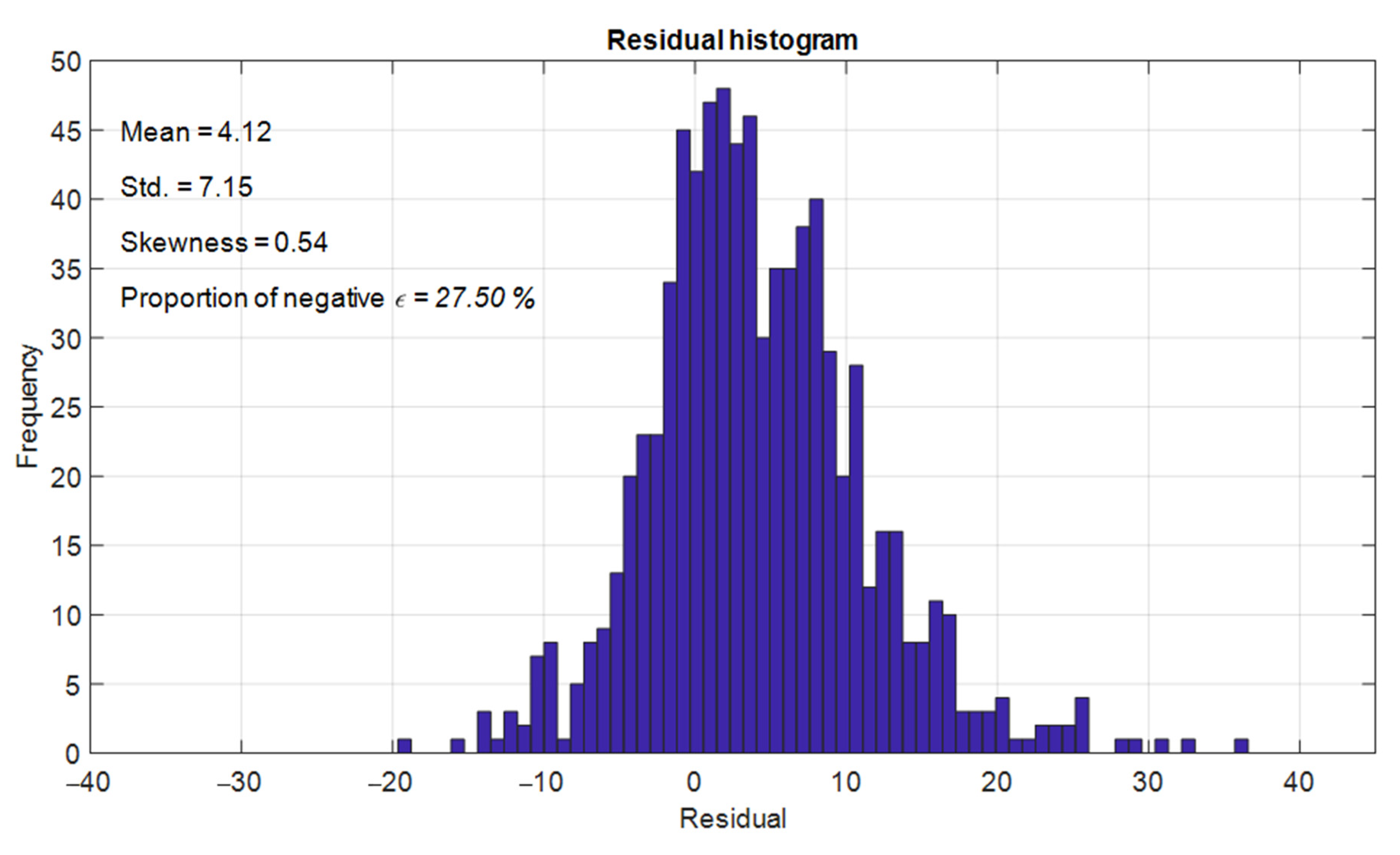
In addition to prediction accuracy, reliability is also a major concern in CS estimation [38,39]. Restriction of overestimation is an important task in model building. However, improving the reliability of the estimation has rarely been addressed in the case of HPC. The current work is an attempt to fill this gap in the literature. An asymmetric loss function is utilized in the training phase of the XGBoost regressor to express the bias against overestimations. By doing so, the number of overestimated CS values can be reduced, and the model’s reliability is enhanced accordingly. Additionally, XGBoost-based quantile regression is used to derive the prediction interval of the CS values.

(v)

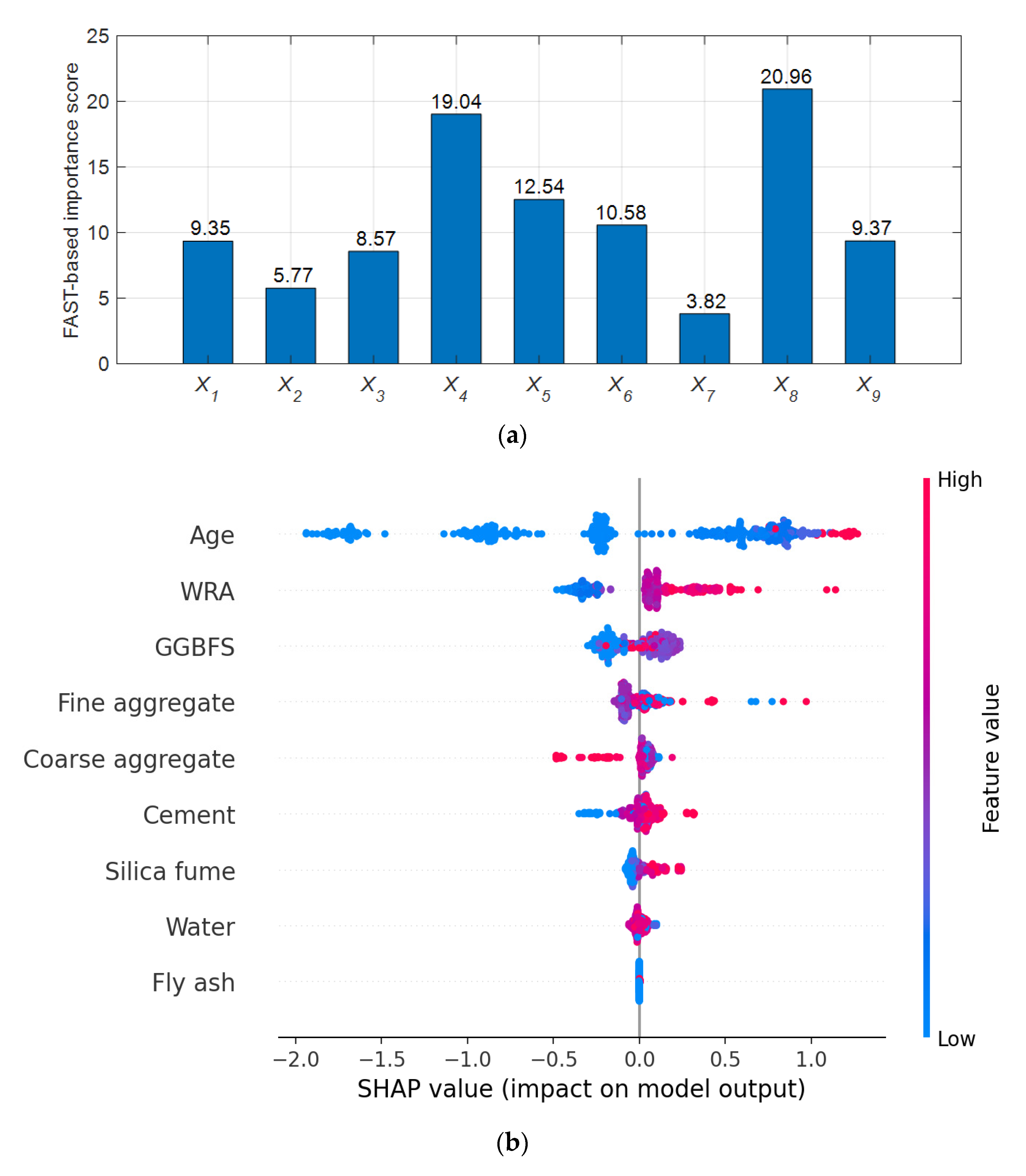
To assess the contribution of predictor variables to the model’s output, this study resorts to the Fourier Amplitude Sensitivity Test. This is a variance-based global sensitivity analysis approach for computing the effects of the input factors on the CS of HPC. This test helps identify the constituents that considerably affect the response.

(vi)

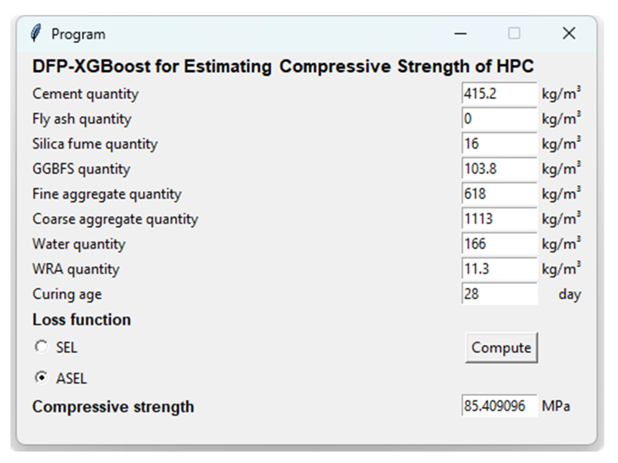
A program based on DFP-XGBoost with a graphical user interface has been developed in Python to ease the implementation of the model. Using this program, the user can obtain a prediction of the CS of untested HPC mixes.

3. Research Method

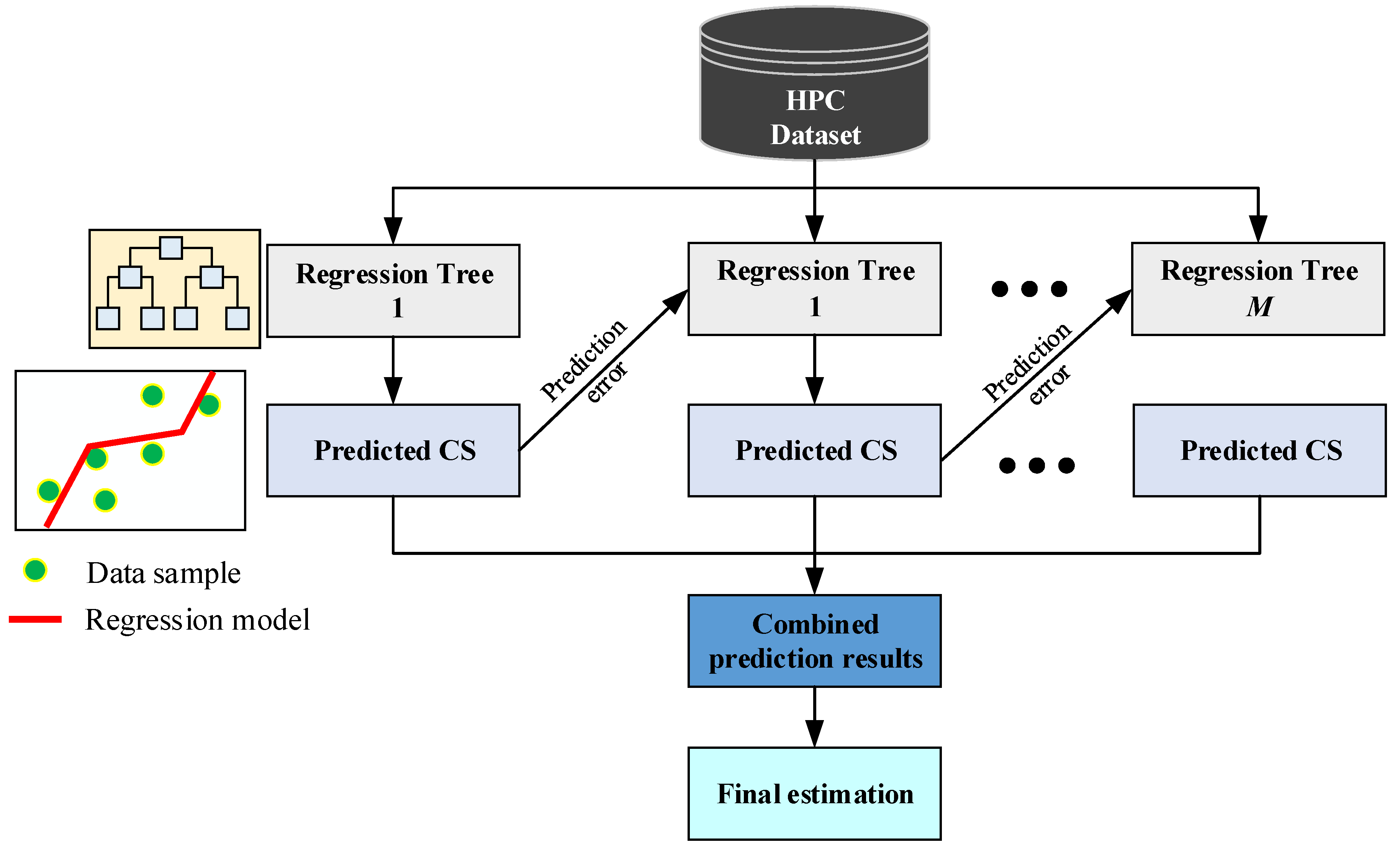
3.1. Extreme Gradient Boosting Machine Regressor

The Extreme Gradient Boosting Machine (XGBoost), put forward in [36], is widely considered as a powerful ensemble learning approach for nonlinear and multivariate function approximations [23,24]. This regressor gradually improves a single weak regression tree by combining it with other individual models to establish a collectively robust model. Iteratively, the prediction error of the previous weak learners is fitted by the next one. Herein, XGBoost implements a process of adding weak models to its ensemble in which the learning phase is formulated as a gradient descent algorithm over an objective function. The overall structure of an XGBoost model is demonstrated in Figure 1.

The objective function of XGBoost can be expressed as follows [18,36]:

$$f_{obj}={\displaystyle {\sum }_{i}L(y_i,F(x_i))}+{\displaystyle {\sum }_k\Omega (f_k)}$$

(1)

where $\Omega (f)=\gamma T+\frac{1}{2}\lambda {\displaystyle \sum _j^T{w}_j^2}$ is the regularization term; T denotes the leaf number in a regression tree f; w_j is the score of a leaf j; $\gamma$ represents a threshold of the score function used for splitting regression trees. $\lambda$ denotes a regularization coefficient.

To compute f_obj, it is required to specify a loss function. For regression analysis, the commonly used loss function is the squared error loss (SEL) [40], which is expressed as follows:

$$L(t,y)={(t-y)}^2$$

(2)

where t and y denote the actual and forecasted values of the response, which is the CS of HPC mixes.

To find a solution for the aforementioned optimization problem, a Taylor’s second-order approximation is employed. In addition, the first- and second-order gradients of the loss function L(t, y) must be computed. Accordingly, the optimal score of each leaf in a decision tree can be expressed as follows [18]:

$$w_j^{*}=-\frac{{\displaystyle {\sum }_{i\in I_j}{g}_i}}{{\displaystyle {\sum }_{i\in I_j}{h}_i+\lambda }}$$

(3)

where g_i and h_i represents the first- and second-order gradients of L(t, y), respectively, and $I_j$ denotes the data instances that arrive at a leaf.

After being trained, an XGBoost model used for CS estimation is given by:

$$F_{XGBoost}={\displaystyle \sum _{k=1}^M{f}_k(x)}$$

(4)

where M denotes the number of individual models in the ensemble; x is the feature vector of the model, which describes the characteristics of a HPC mixes; F_XGBoost is the CS value of the mix estimated by XGBoost.

Notably, XGBoost offers various advantages over other ensemble approaches in model building. As pointed out in [41], this boosting machine employs a smart tree-splitting mechanism and an efficient randomization method for enhancing the diversity of the collective model. In addition, regularization terms can be incorporated into the objective function of XGBoost to make this model more resilient to overfitting. This boosting machine also implements a level-wise strategy to assess the quality of possible splits across the training set. Therefore, XGBoost models are able to minimize both variance and bias effectively. Last but not least, the training process of XGBoost can be executed parallelly on graphics processing units. This feature makes XGBoost scalable and allows it to cope well with large-scale datasets.

3.2. Differential Flower Pollination

Differential Flower Pollination (DPF), put forward in [37], is a nature-inspired metaheuristic algorithm. DFP is designed to combine the searching operations of Differential Evolution (DE) [42] and the Flower Pollination Algorithm (FPA) [43]. This metaheuristic relies on DE for exploitation of the search space and the FPA for enhancing the exploration capability. In the current work, DFP is used for automating the model selection phase of the XGBoost regressor. This task is formulated as a global optimization problem in which the hyper-parameters of XGBoost are modeled as decision variables. An objective function expressing the model’s predictive capability is used to guide the population of the metaheuristic approach to the optimal solution. DFP inherits effective searching operators from DE, including mutation and cross-over. Moreover, it employs a Levy flight-based global search as described in the FPA [43]. DFP is particularly suitable for optimizing the performance of machine learning models because it is a gradient-free method and possesses good search capability [44]. For more details regarding the implementation of DFP, readers are guided to the previous works of [37,44].

3.3. The Collected Dataset

Since the CS estimation is modeled as a supervised learning task, the preparation of data samples containing actual laboratory test results is crucial. These data samples provide the features and expected values of the response. Herein, the features consist of the mixes’ constituents and testing age. The response is the testing outcome of the mixes’ CS. To train the XGBoost regressor, this study has conducted a comprehensive literature survey and gathered data samples from the current literature. The independent variables in the study are selected via the findings of previous works [8,13,14,45] as well the availability of data. Those variables are used as inputs for the machine learning model to estimate the CS of HPC measured in MPa. Due to the availability and compatibility of data, other influencing factors, such as curing conditions and the size distribution of aggregates, have not been considered in the current work.

Moreover, the selection of the data samples is based on the recommendations of the w/c ratio as well as the total content of the cementitious materials in [5,6]. To ensure the quality of the laboratory testing results, the data samples are collected from reliable academic articles. After the literature review process, a historical dataset, consisting of 400 data points, is established. The sources of the data samples are reported in

Table 1. Data sources.

Data Source	Number of Laboratory Tests	Proportion (%)	Type of Specimens	Reference
1	100	25.00	150 × 150 × 150 mm cube	[16]
2	4	1.00	100 × 200 mm cylinder	[46]
3	16	4.00	100 × 100 × 100 mm cube	[47]
4	52	13.00	100 × 100 × 100 mm cube	[10]
5	28	7.00	100 × 100 × 100 mm cube	[14]
6	200	50.00	150 × 300 mm cylinder	[6]

. It is noted that the specimen sizes in different data sources are inconsistent. Therefore, this study relies on correlation factors [38] to standardize the CS values. The correlation factors are provided in

Table 2. Correlation factors used for standardizing the compressive strength values.

Specimen	Cube	Cube	Cylinder	Cylinder
Dimension (mm)	150 × 150 × 150	100 × 100 × 100	100 × 200	150 × 300
Correlation factor	1.119	1.000	1.020	1.063

. The statistical descriptions of the variables in the dataset are summarized in

Table 3. Statistical description of the variables.

Variables	Unit	Notation	Min	Average	Std	Skewness	Max
Cement content	kg/m3	X1	80.00	378.16	103.28	−1.38	527.20
Fly ash content	kg/m3	X2	0.00	6.42	22.56	3.51	123.50
Silica fume content	kg/m3	X3	0.00	19.93	21.63	0.71	75.00
GGBFS content	kg/m3	X4	0.00	96.40	84.87	1.19	360.00
Fine-aggregate content	kg/m3	X5	488.00	649.20	79.25	0.07	804.96
Coarse-aggregate content	kg/m3	X6	915.20	1129.35	48.23	−1.33	1203.00
Water content	kg/m3	X7	120.00	161.13	14.45	−1.52	180.00
WRA content	kg/m3	X8	1.30	9.42	4.18	−0.07	18.00
Age	day	X9	1.00	48.68	91.37	2.93	400.00
Compressive strength	MPa	Y	22.54	69.66	22.13	−0.06	120.86

Note: Std denotes the standard deviation.

.

In the collected dataset, the contents of cement, fly ash, silica fume, GGBFS, fine aggregate, coarse aggregate, water, water-reducing agent (WRA), and curing age are employed as influencing variables. The use of Supplementary Cementing Materials, including silica fume, fly ash, and GGBFS, is crucial for HPC mixes to modify their mechanical performance. Silica fume is a highly pozzolanic material that is capable of improving the strength and durability of concrete. Fly ash and GGBFS are by-products of industrial processes that are also widely used to enhance the mechanical properties and sustainability of concrete [48,49,50,51]. In addition, since HPC generally requires low w/c ratios, a WRA (e.g., high-range water reducers and superplasticizers) is commonly employed to reduce the water content and ensure the workability of concrete mixes [5,6].

3.4. Benchmark Methods

3.4.1. Artificial Neural Network

The artificial neural network (ANN) is a machine learning approach inspired by actual biological brains in the natural world [52]. ANNs have been widely used for CS estimation, and positive results obtained from this method were reported in various studies [9,27]. A typical ANN model consists of an input, a hidden layer, and an output layer. The first layer receives input signals that contain the characteristics of a concrete mixture. These input signals are then transmitted to the neurons in an ANN’s hidden layer, where various data transformation and feature engineering processes are performed. To deal with nonlinear functional mappings, the ANN relies on activation functions (e.g., the sigmoid function) to process the input data of a neuron. The output layer yields the estimated CS values based on the signals arriving at the input layer. To construct an ANN model for predicting the CS of HPC, its structure, specified by the synaptic weights, must be trained. Based on previous studies [16,53], the current paper resorts to the Levenberg–Marquardt algorithm for constructing the ANN model.

3.4.2. Support Vector Regression

Support vector regression (SVR) is also a popular machine learning approach used for CS estimation [21,27]. This method constructs a mapping function by identifying a set of crucial data samples within the training set. These crucial data samples help locate the inference model and are called support vectors. Notably, only a small fraction of the training samples are selected to construct an SVR model. Therefore, SVR can achieve both the objectives of low prediction error and good sparseness. The reason is that a sparse model is less affected by noise. In addition, SVR employs the epsilon-insensitive loss function during its training process. Using this loss function, prediction errors that are less than a certain limit (${\epsilon }_{SVR}$) are not penalized by the model. The training process of an SVR model is formulated as a quadratic programming problem that can be solved by a nonlinear programming solver. To deal with nonlinear mapping, SVR relies on kernel functions to perform data transformations. The radial basis function is often employed for regression analysis [54].

4. Result and Discussion

4.1. Experimental setting

As stated in the previous section, the dataset, consisting of 400 samples and nine independent variables, is employed to train and validate the machine learning methods. This study randomly divides the collected data samples into two sets: the training set (90%) and the testing set (10%). The former is used to construct the proposed approach, named DFP-XGBoost. The latter, which includes 40 samples, is reserved to inspect the model’s generalization property. Since the model optimization of DFP-XGBoost requires the fine-tuning of various hyper-parameters, this study allocates 90% of the samples in the training set to provide sufficient data for the model construction phase.

Due to the effect of randomness in data sampling, one experiment with the model’s training and testing may not be sufficient for evaluating its forecasting capability. Hence, this study has performed the experiment with DFP-XGBoost 20 times. In each experiment, 10% of the collected samples are randomly drawn to serve as untested concrete mixes. The rest of the dataset is used for model construction. Since the variables in the dataset have different ranges, the variables with large magnitudes may dominate the others. To avoid this situation, a data normalization technique should be employed to pre-process the dataset. This study relies on the Z-score normalization method for standardizing the ranges of variables. The Z-score normalization equation is given by:

$$X_Z=\frac{X_O-{\mu }_X}{{\sigma }_X}$$

(5)

where $X_Z$ and $X_O$ denote the normalized and original variables, respectively. It is noted that the variables include all the input features as well as the CS of HPC. ${\mu }_X$ and ${\sigma }_X$ are the mean and standard deviation (std) of the original variables, respectively.

Moreover, to assess the performance of the prediction models, the root mean square error (RMSE), mean absolute percentage error (MAPE), and coefficient of determination (R²) are used in this section. RMSE is essentially the quadratic mean of the discrepancy between the actual compressive strength values (measured from destructive testing) and the estimated ones (yielded by the machine learning models). RMSE is non-negative; the closer it is to 0, the better the prediction accuracy. MAPE computes the average magnitude of errors estimated by the machine learning model. This index varies from 0 to 100%. As pointed out by [24], MAPE less than 10% indicates excellent performance; values in the range of [10%, 20%] show good performance. Therefore, it is expected that a decent prediction model for the CS estimation of HPC mixes should have MAPE <20%. In addition, R² exhibits the proportion of the variation in the CS that can be explained by the machine learning approach; it ranges from 0 to 1. The larger the value of R2, the more predictive the model is.

These indices were selected in this study because they are commonly used for performance measurement and comparison in previous works related to the compressive strength estimation of concrete mixes [24,26,30]. The metrics of RMSE, MAPE, and R² are given by:

$$RMSE=\sqrt{\frac{1}{N}{\displaystyle \sum _{i=1}^N{(y_i-t_i)}^2}}$$

(6)

$$MAPE=\frac{100}{N}\times {\displaystyle \sum _{i=1}^N\frac{|y_i-t_i|}{y_i}}$$

(7)

$$R^2=1-\frac{{\displaystyle \sum _{i=1}^N{(t_i-y_i)}^2}}{{\displaystyle \sum _{i=1}^N{(t_i-\overline{t})}^2}}$$

(8)

where t_i and y_i are the actual and forecasted CS of an HPC mix, respectively. N denotes the number of data samples.

It is noted that the proposed method is a combination of DFP and XGBoost. The DFP metaheuristic is employed to optimize the performance of the XGBoost regressor by identifying the most suitable set of its hyper-parameters. The predictive capability of XGBoost strongly depends on the number of individual trees (M) in the ensemble, the learning rate, the maximum tree depth (MTD), the L₂-regularization parameter $(\lambda )$, and the L₁-regularization parameter $(\alpha )$. The number of individual trees and MTD significantly control the predictive power of XGBoost. The larger the values of M and MTD are, the more degrees of freedom the model has.

Sophisticated models are capable of explaining the complex mapping relationship between the predictor variables and the response. However, an excessively sophisticated model tends to suffer from overfitting. An overfitted model may achieve a desired goodness of fit in the training phase, but it may perform unsatisfactorily on unseen data samples. To avoid overfitting, the regularization parameters ($\lambda$ and $\alpha$) should be used. The larger those regularization parameters are, the more restricted the complexity of the model is. This study relies on DFP to automatically search for the most appropriate values of the five hyper-parameters of XGBoost.

To implement DFP, an objective function that expresses the model’s quality must be defined. Accordingly, the following objective function is used during the optimization process of DFP:

$$f={\displaystyle \sum _{k=1}^K(\frac{RMS{E}_{Tr}+RMS{E}_{Te}}{K})}+\chi \times (M+MTD)+\rho \times (\frac{1}{1+\lambda }+\frac{1}{1+\alpha })$$

(9)

where ${\displaystyle \sum _{k=1}^K(\frac{RMS{E}_{Tr}+RMS{E}_{Te}}{K})}$ denotes the model performance obtained from a cross-validation process with K = 5; RMSE_Tr and RMSE_Te are the prediction errors in the training and testing phases, respectively; $\chi$ and $\lambda$ are weighting coefficients.

The objective function described in Equation (9) guides DFP to search for a model’s configuration that features a fine balance between low prediction error and a high generalization property. Since these two goals are often conflicting in nature, the use of DFP is particularly helpful for the model-building process. The weighting coefficients in Equation (9) can be identified experimentally. Via several trial-and-error runs, the suitable values of $\chi$ and $\lambda$ were found to be 0.01 and 0.001, respectively. It is noted that the lower boundaries of M, the learning rate, MTD, $\lambda$, and $\alpha$ are 1, 0.01, 1, 0, and 0, respectively. Their upper boundaries are 100, 10, 10, 100, and 100. The DFP metaheuristic is coded in Python by the author. Meanwhile, the XGBoost regressor is built using the toolbox provided in [55].

To demonstrate the advantages of DFP-XGBoost, an ANN and SVR, two commonly employed models for CS estimation, are used. The ANN model is trained by the Levenberg–Marquardt algorithm and built in MATLAB’s neural network toolbox [56]. The SVR model is constructed with the built-in functions provided in the scikit-learn machine learning library [57]. The hyper-parameters of the ANN and SVR are set via five-fold cross-validation processes [58]. In detail, the number of neurons in the hidden layer of the ANN model and its learning rate are selected to be 18 and 0.001, respectively. This model was trained for 300 epochs. In addition, the hyper-parameters of SVR, including the penalty coefficient (C_SVR), the kernel function parameter (K_SVR), and the radius of the epsilon-insensitive tube $({\epsilon }_{SVR}),$ are set to be 400, 0.1, and 0.05, respectively. It is noted that experiments with the machine learning models in this paper were conducted on a Dell G15 5511 (Core i7-11800H and 16 GB RAM).

4.2. Prediction Results and Performance Comparison

As stated earlier, the hybrid model employs the DFP metaheuristic to fine-tune its hyper-parameters (i.e., the number of individual trees, learning rate, MTD, and regularization coefficients). DFP was implemented with 20 members in its population and executed for 100 generations. In the first generation, the population of DFP is generated randomly within its boundaries. This algorithm uses mutation, crossover, and Lévy flight-based global search operations to exploit and explore the search space. The evolutionary process of DFP used for optimizing the performance of the XGBoost regressor is demonstrated in Figure 2. The optimized model’s hyper-parameters are found as follows: M = 12, learning rate = 1.42, MTD = 4, $\lambda =98.62$, and $\alpha =0.013$.

Table 4. Performance of the machine learning models.

Phase	Performance Measurement Indices	DFP-XGBoost		ANN		SVR
		Mean	Std	Mean	Std	Mean	Std
Training	RMSE	3.710	0.148	6.746	2.649	7.424	0.106
	MAPE (%)	4.780	0.183	8.857	4.040	9.852	0.164
	R2	0.972	0.003	0.893	0.076	0.887	0.004
Testing	RMSE	5.270	0.834	8.823	1.990	10.461	1.204
	MAPE (%)	6.740	1.360	11.836	3.350	15.212	2.037
	R2	0.942	0.020	0.820	0.096	0.763	0.053

summarizes the prediction outcomes of DFP-XGBoost and other benchmark models in terms of all performance measurement metrics. It is observable that the proposed method has achieved the best results with an RMSE of 5.270, an MAPE of 6.740%, and an R² of 0.942. The ANN is the second-best method, with an RMSE of 8.823, an MAPE of 11.836%, and an R² of 0.820. The result of SVR (RMSE = 10.461, MAPE = 15.212%, and an R² of 0.763) is inferior to that of DFP-XGBoost and the ANN. To quantify the correlation between the actual and estimated results, the R² index can be used. This index is also an indicator of the proportion of the variation in the CS of HPC that can be estimated from DFP-XGBoost and its influencing variables. With an R² of 0.94, the prediction results are satisfactory because the hybrid model is capable of explaining 94% of the variation in the output variable. Moreover, the ANN and SVR are only capable of explaining 82% and 76% of the variation in the modeled variable. Figure 3 graphically shows the improvements in results obtained by DFP-XGBoost. The newly developed method helps decrease roughly 40% and 43% of the prediction errors in terms of RMSE and MAPE, respectively. In terms of R², DFP-XGBoost achieves a 14.88% improvement compared with other methods.

Considering the aspect of computational cost, the DFP-based optimization requires roughly 236 s to complete its evolutionary process. However, the DFP-XGBoost’s prediction phase can be executed very fast in roughly 0.5 s. The cross-validation processes used by the ANN and SVR require a computation time of 68.6 s and 13.3 s. The prediction phases of the ANN and SVR can be accomplished in 0.06 s and 0.70 s, respectively. It can be seen that DFP-XGBoost employs the DFP metaheuristic for model optimization. Hence, the computation time of its model construction phase is significantly longer than that of the benchmark approaches. The reason is that DFP is a population-based evolutionary algorithm; it necessitates a large number of cost function evaluations during the optimization process.

In addition, Figure 4 provides more insights regarding the distribution of the residual range (r) of the prediction models. It is noted that the range of residuals has been normalized by the magnitude of the actual CS values. Herein, the values of r obtained from each model are divided into five categories: (i) r ≤ 5%, (ii) 5% < r ≤ 10%, (iii) 10% < r ≤ 15%, (iv) 15% < r ≤ 20%, and (v) r > 20%. As pointed out in [24], a relative error of less than 20% can be considered satisfactory for the task of CS estimation. Meanwhile, the relative error less than 10% indicates excellent prediction outcomes. Moreover, comparing the distribution of prediction errors can bring about better understanding of the predictive capability of the machine learning model [40].

As can be seen from Figure 4, DFP-XGBoost achieves the highest proportion of the data samples in the first category (54.75%). This outcome is better than SVR (38.12%) and ANN (36.5%) by a large margin. The proportions of residual ranges in the second group of DFP-XGBoost and the ANN are relatively equal. Meanwhile, the number of residual ranges in (10%, 15%] yielded by the ANN is larger than that obtained from other models. Notably, 80.25% of the results predicted by DFP-XGBoost have an error range of less than 10%. The proportion of interest for the ANN and SVR models is 61.62% and 57.50%, respectively. Data samples in the last category only occupy 5.12% in the case of DFP-XGBoost. Meanwhile, this proportion of data samples yielded from the benchmark methods is at least three times larger than that of the proposed method. These analyses point out the highly satisfactory performance of DFP-XGBoost regarding the distribution of the residual range.

Furthermore, the boxplots in Figure 5 illustrate the minimum, first quartile, median, third quartile, and maximum of the RSME values obtained from the prediction models. A red line in each distribution denotes the median of the prediction errors. The median of prediction errors for DFP-XGBoost is 5.11 MPa, which is significantly below that of the ANN (8.47 MPa) and SVR (10.26 MPa). In addition, Wilcoxon signed-rank tests [59] are used to compare the performance of the models used for predicting the CS of HPC. The threshold of the p-value of the tests is set to be 0.05. The hypothesis tests of DFP-XGBoost vs. the ANN and DFP-XGBoost vs. SVR both yield p-values of 0.0001, which is lower than the selected threshold. Therefore, there is sufficient confidence to reject the null hypothesis of equal performance and confirm the superiority of the proposed DFP-XGBoost over the benchmark approaches.

4.3. Sensitivity Analysis-Based Assessment of Feature Importance

For CS estimation, the relative influence of the independent variables on the response is helpful for the mixture design process. To clarify the influence of the predictor variables on the DFP-XGBoost’s output, this study relies on the global analysis of the Fourier Amplitude Sensitivity Test (FAST) [60] as well as the SHAPley Additive exPlanations (SHAP) [61]. FAST is a popular method for revealing the relative influence of a model’s input variables over its prediction accuracy [38]. Based on the test’s result, the sensitivity values of the variables can be calculated to express their relative importance. In this study, the Python toolbox provided in [62] is used to perform the sensitivity test. Meanwhile, SHAP is the approach for elucidating the model’s structure. This method is often used to express the effect of each feature on the predicted outcome. The SHAP approach is performed with the Python library developed by Lundberg [63].

The outcome of the analyses is presented in Figure 6. Based on FAST, four out of nine variables have significant effects on the CS of HPC, namely X₈ (quantity of WRA), X₄ (quantity of GGBFS), X₅ (quantity of fine aggregate), and X₆ (quantity of coarse aggregate). Concrete age (X₉), cement content (X₁), and silica fume (X₃) demonstrate moderate impacts on the response. Meanwhile, the relative importance of fly ash content and water content is lower than other variables. Based on SHAP, we are able to categorize the features into three groups according to their order of importance. The first group includes the curing age, quantity of WRA, quantity of GGBFS, and quantity of fine aggregate. The dosages of coarse aggregate, cement, and silica fume can be categorized into the second group. Meanwhile, the third group consists of water content and fly ash content. Thus, the results of SHAP are, to some degree, in agreement with those of FAST. Both methods emphasize the importance of the WRA in HPC mix design.

4.4. Interval Prediction of Compressive Strength Based on Quantile Regression

The standard XGBoost regressor is capable of providing point estimates of the CS values. Although the previous section demonstrates that this model can achieve outstanding prediction results with an RMSE of 5.72 and an MAPE of 6.74%, it cannot yield information about the dispersion of the predictions around the CS value. This study resorts to quantile regression [64] for expressing a functional relationship between the independent variables (i.e., the mix’s constituents and curing age) for all possible portions of a probability distribution. Quantile regression can be used to derive prediction intervals from a base model [65]. For instance, a 95% prediction interval for the estimated CS can be expressed as follows:

$$PI(x)=[Q_{0.025}(x),Q_{0.975}(x)]$$

(10)

where $Q_{0.025}(x)$ and $Q_{0.975}(x)$ are the two XGBoost models trained with the quantile regression parameters of 0.025 and 0.975, respectively.

Hence, to derive the interval estimation of the CS of HPC, it is required to train two separate XGBoost regressors that employ two quantile regression parameters. By doing so, DFP-XGBoost is able to yield a range estimation of the CS values in addition to their point estimation. To construct these two models, the first-order derivative of the loss function of the model is revised as follows [66]:

$$\frac{\partial L}{\partial y}=\left\{\begin{array}{c}{\zeta }_{QR}if\epsilon >0\hfill \\ {\zeta }_{QR}-1if\epsilon <0\hfill \\ 0if\epsilon =0\hfill \end{array}\right.$$

(11)

where ${\zeta }_{QR}$ denotes the quantile regression’s parameter; $\epsilon$ is the model’s residual; y denotes the predicted CS value.

In addition, to evaluate the quality of prediction intervals, prediction interval coverage probability (PICP) can be computed [67]. PICP basically measures the proportion of the predicted CS values that lie within the lower and upper boundaries. In addition, the mean width of the prediction interval (MWPI) is an index that characterizes the width of the interval estimation. The PICP is expected to be as close to the specified confidence level as possible. Meanwhile, the MWPI should be reasonably narrow to convey useful information about the range estimation of the CS. This study constructs 95% interval estimations of the CS values by integrating XGBoost and the quantile regression method. Herein, the XGBoost model used for deriving the lower bound of the estimations is built with ${\zeta }_{QR}$ = 0.025. Meanwhile, the one that yields the upper bound of the estimations is trained with ${\zeta }_{QR}$ = 0.975. The prediction intervals for one experiment with 40 testing samples are illustrated in Figure 7. Considering the estimation results obtained from 20 runs, the average PICP and MWPI in the training phases are 96% and 28.49 MPa, respectively. These values obtained from the testing phases are 84% and 28.25 MPa. Hence, the MWPIs in the training and testing phases are relatively equal to each other. Although the PICP in the training phase is satisfactory, the result in the testing phase could not meet expectations. This result can be explained by the fact that the uncertainty of the response in the testing phase is much higher than that in the training phase. Therefore, the model has failed to reach a PICP of 95% for novel data samples.

4.5. Reduction in Overestimations Committed by XGBoost Regressor

In CS estimation, besides the goal of minimizing the prediction errors or residuals, enhancing the model’s reliability is also of practical concern. The standard loss function used for training an XGBoost regressor (i.e., the SEL) is symmetric in nature. Therefore, it treats negative and positive errors similarly during the training process. Notably, the model residual ($\epsilon$) is calculated as t − y, where t and y denote the actual and predicted CS values, respectively. If the actual CS is less than the estimated one, the residual is negative, and the model overestimates the target variable. This situation is undesirable because it leads to unsafe prediction outcomes. Therefore, negative residuals or overestimations should be avoided [39].

Because SEL is symmetric, the proportions of negative and positive residuals of the model trained by the XGBoost regressor using SEL are expected to be similar. By inspecting the actual and estimated CS values in multiple experiments, the percentage of negative residuals is found to be 47.12%. Therefore, the numbers of overestimated and underestimated results are relatively equal to each other. The distribution of the residuals obtained from the model using SEL is demonstrated in Figure 8. The mean, standard deviation, and skewness of the distribution are found to be 0.07, 5.34, and $-$0.87, respectively. Hence, the average of the errors is close to 0. In addition, a negative skewness of $-$0.87 indicates that the left tail of the distribution is longer than the right one. This fact is also confirmed by visually inspecting the histogram in Figure 8. To enhance the reliability of the model, it is desired to shorten the left tail of the distribution because data samples in this region are associated with overestimated results. Figure 9 shows more details of the model’s residuals; the average magnitude of the negative residuals (4.13 MPa) is slightly higher than that of the positive ones (3.80 MPa).

To express the bias against overestimations, the asymmetric squared error loss (ASEL) should be used for training XGBoost [40]. The ASEL function, denoted as $L_{ASEL}$, is given by:

$$L_{ASEL}(t,y)=\left\{\begin{array}{c}{(t-y)}^2,if(t-y)\ge 0\hfill \\ \rho \times {(t-y)}^2,otherwise\hfill \end{array}\right.$$

(12)

where $\rho$ is a tuning parameter of the function for controlling the degree of asymmetry. The larger the value of $\rho$, the more severe overestimations are penalized.

To implement the ASEL with the XGBoost regressor, its first-order and second-order derivatives of the loss function with respect to the predicted result (y) are revised in the following manner [40]:

First-order derivative:

$$L^{\prime }(t,y)=\left\{\begin{array}{c}2\times (t-y),if(t-y)\ge 0\hfill \\ 2\times \rho \times (t-y),otherwise.\hfill \end{array}\right.$$

(13)

Second-order derivative:

$$L^{\prime \prime }(t,y)=\left\{\begin{array}{c}2,if(t-y)\ge 0\hfill \\ 2\times \rho ,otherwise\hfill \end{array}\right.$$

(14)

The ASEL generally imposes a large penalty on overestimated results. Therefore, the model is trained to maximize the number of positive residuals. However, fine-tuning of $\rho$ is necessary because excessively large values of this parameter may significantly impair the overall prediction accuracy of the model. The experimental results with different values of $\rho$ are reported in Figure 10. As $\rho$ increases from 0 to 15, the proportion of underestimations gradually rises. However, the overall predictive capability of the model, expressed in terms of R², tends to be damaged. Observable from the figure, with $\rho$ = 10, the percentage of positive residuals reaches 72.5% and the model can capture up to 85% of the variability in the CS of HPC. When the parameter of the ASEL surpasses 10, the gain in proportion of positive residuals is insignificant; meanwhile, the overall performance of the model deteriorates considerably. Therefore, $\rho$ = 10 is selected for the XGBoost regressor in this study.

Using the ASEL with $\rho$ = 10, the performance of DFP-XGBoost regarding the characteristics of its residuals is significantly improved. As shown in Figure 11, the average value of the residuals increases from roughly 0.7 to 4.12. The bulk of the distribution shifts to the right side of the horizontal axis. Therefore, the number of overestimations is considerably reduced from 47.12% to 27.5%. In other words, underestimations account for 72.5% of the prediction. The skewness of the distribution also changes sign; this fact indicates that its right tale is longer than the left one. It is highly desirable for CS estimation because the magnitude of overestimation has been reduced. However, the use of the ASEL also causes a certain increase in the range of positive residuals. As demonstrated in Figure 12, the average range of positive residuals increases from 3.80 MPa to 7.12 MPa. On the contrary, the average range of negative ones decreases from 4.13 MPa to 3.80 MPa.

The prediction results of DFP-XGBoost trained by the ASEL (denoted as DFP-XGBoost-ASEL) are demonstrated in Figure 13. As observed in the figure, the majority of the data points are located below the line of best fit. This fact accounts for the high proportion of underestimations. DFP-XGBoost-ASEL is able to achieve an RMSE of 8.13, an MAPE of 9.57%, and an R² of 0.852. Notably, the MAPE of the model is still less than 10%, which indicates good prediction performance in CS estimation [24]. Detailed performance of the models using the two loss functions are provided in

Table 5. Comparison of the model’s performance using SEL and ASEL.

Phase	Performance Measurement Indices	DFP-XGBoost Using SEL		DFP-XGBoost Using ASEL
		Mean	Std	Mean	Std
Training	RMSE	3.710	0.148	6.280	0.648
	MAPE (%)	4.780	0.183	7.290	0.855
	R2	0.972	0.003	0.919	0.017
Testing	RMSE	5.270	0.834	8.130	1.360
	MAPE (%)	6.740	1.360	9.570	1.630
	R2	0.942	0.020	0.852	0.054

. Based on the experimental results, the use of the ASEL brings about a reduction in the model’s performance in both the training and testing phases. The Wilcoxon signed-rank test yields a p-value of 0.00009 < 0.05, confirming that the overall predictive accuracy of DFP-XGBoost-ASEL is statistically lower than that of the one using the SEL. Nevertheless, the former also helps significantly restrict the occurrence of overestimations. Therefore, there is an inevitable trade-off between overestimation reduction and prediction error minimization.

One notable observation is that although DFP-XGBoost-ASEL is inferior to the standard XGBoost regressor, it still outperforms other benchmark methods in terms of all measurement indices. Therefore, the proposed method is a promising alternative for assisting researchers and construction engineers in HPC mix design and prediction of the mix’s mechanical properties. Furthermore, to ease the implementation of DFP-XGBoost, a graphical user interface (GUI) has been developed in Python (v. 3.10). The model’s GUI is provided in the Appendix A of this paper and the Github repository. It is noted that the program is constructed with the assistant of the tkinter package [68]. The developed program is able to provide the user with estimated CS values of untested HPC mixes. The required input information includes the mix’s constituents and curing age. Both the SEL and ASEL can be selected in the GUI via the setting of the radio buttons.

5. Conclusions

The estimation of the CS of HPC is crucial for the tasks of mix design. This study has proposed and verified a hybrid data-driven approach named DFP-XGBoost for enhancing the accuracy as well as the reliability of the CS estimation model. In this integrated framework, XGBoost is employed as a regressor for generalizing a functional mapping between the CS of HPC mixes and their influencing variables. The quantities of cement, Supplementary Cementitious Materials (i.e., silica fume, GGBFS, fly ash), water, fine aggregate, coarse aggregate, and WRA are utilized as independent variables regarding the mixes’ constituents. It is noted that forecasts of the CS at different curing times are also important for studying the developmental progress of the concrete’s properties. In addition, this capability is also helpful for scheduling construction activities related to the removal of formwork systems and the re-shoring of reinforced concrete slabs. Hence, this study also considers the concrete age as an input feature of the machine learning model.

To automate the model construction phase, this study relied on the DFP metaheuristic algorithm. DFP helps carry out the model selection phase of XGBoost in an entirely data-driven manner. Based on the model’s performance on the training dataset, DFP guides a population of the model’s hyper-parameters to a good solution that minimizes the objective function. In this manner, the model’s hyper-parameters, including the number of trees, learning rate, maximum tree depth, L₂-regularization coefficient, and L₁-regularization coefficient, can be adapted entirely by the collected data without the need for human intervention. A historical dataset consisting of 400 samples was gathered from previous works to construct DFP-XGBoost. After being trained, the model is able to yield estimated CS values for untested HPC mixes. Additionally, a program with a simple GUI is developed in Python to ease the implementation of the proposed approach.

Experimental results show that the hybrid model has achieved an outstanding result with an RMSE of 5.27, an MAPE of 6.74%, and an R² of 0.94. This performance is highly desirable because DFP-XGBoost is capable of explaining up to 94% of the variability in the CS of HPC. To reduce the number of overestimations, this study resorts to the ASEL function for training the XGBoost regressor. As can be seen from the experimental results, the use of the ASEL helps decrease the percentage of overestimated CS values by 19.62%. However, this reduction in overestimation is achieved by a certain compromise in the overall prediction accuracy. Moreover, XGBoost-based quantile regression for estimating the CS of HPC is also investigated in this study. By modifying the loss function of XGBoost, this model is capable of yielding prediction intervals of CS values at a certain confidence level. Accordingly, the proposed hybrid approach can be a capable and reliable tool for assisting with the tasks of mixture design and optimization. The newly developed DFP-XGBoost can be implemented easily and can be applied to model other important mechanical properties of HPC, such as tensile strength and modulus of elasticity.

Nevertheless, the current work also has several limitations. First, the number of mixtures containing fly ash in the dataset is limited. Only 8% of the samples use fly ash as one of the Supplementary Cementitious Materials. Second, the current paper has not considered the use of nanomaterials (e.g., nanosilica) and recycled aggregates in HPC. Third, the total number of samples in the current dataset is still limited. Fourth, other crucial factors, such as the size distribution of aggregates and curing conditions, have not been taken into consideration. Therefore, future work should focus on extending the current dataset by collecting more data samples containing fly ash and other potential factors. Fifth, although the range estimation of the training phase of DFP-XGBoost is qualified with a PICP of 96% for a confidence level of 95%, the prediction interval constructed in the testing phase can only cover roughly 84% of the actual CS values. It is expected that by increasing the number of laboratory testing results in the database, the generalization capability of the model can be further improved. In addition, other advanced techniques for model optimization and range estimation can be explored to ameliorate the current performance. Finally, the capability of other potential approaches for estimating the CS of concrete mixes, such as the Group Method of Data Handling (GMDH), fuzzy logic, and deep learning, should be investigated to enhance the prediction accuracy.

References

1. Van Damme, H. Concrete material science: Past, present, and future innovations. Cem. Concr. Res. 2018, 112, 5–24. [Google Scholar] [CrossRef]
2. Gagg, C.R. Cement and concrete as an engineering material: An historic appraisal and case study analysis. Eng. Fail. Anal. 2014, 40, 114–140. [Google Scholar] [CrossRef]
3. Chou, J.-S.; Pham, A.-D. Enhanced artificial intelligence for ensemble approach to predicting high performance concrete compressive strength. Constr. Build. Mater. 2013, 49, 554–563. [Google Scholar] [CrossRef]
4. Akhnoukh, A.K.; Buckhalter, C. Ultra-high-performance concrete: Constituents, mechanical properties, applications and current challenges. Case Stud. Constr. Mater. 2021, 15, e00559. [Google Scholar] [CrossRef]
5. Neville, A.; Aïtcin, P.-C. High performance concrete—An overview. Mater. Struct. 1998, 31, 111–117. [Google Scholar] [CrossRef]
6. Videla, C.; Gaedicke, C. Modeling portland blast-furnace slag cement high-performance concrete. ACI Mater. J. 2004, 101, 365–375. [Google Scholar]
7. Wu, L.; Farzadnia, N.; Shi, C.; Zhang, Z.; Wang, H. Autogenous shrinkage of high performance concrete: A review. Constr. Build. Mater. 2017, 149, 62–75. [Google Scholar] [CrossRef]
8. Xue, J.; Briseghella, B.; Huang, F.; Nuti, C.; Tabatabai, H.; Chen, B. Review of ultra-high performance concrete and its application in bridge engineering. Constr. Build. Mater. 2020, 260, 119844. [Google Scholar] [CrossRef]
9. Ben Chaabene, W.; Flah, M.; Nehdi, M.L. Machine learning prediction of mechanical properties of concrete: Critical review. Constr. Build. Mater. 2020, 260, 119889. [Google Scholar] [CrossRef]
10. Li, Q.-F.; Song, Z.-M. High-performance concrete strength prediction based on ensemble learning. Constr. Build. Mater. 2022, 324, 126694. [Google Scholar] [CrossRef]
11. Azkune, M.; Puente, I.; Santilli, A. Shore overloads during shoring removal. Eng. Struct. 2010, 32, 3629–3638. [Google Scholar] [CrossRef]
12. Lee, S.; Nguyen, N.-H.; Karamanli, A.; Lee, J.; Vo, T.P. Super learner machine-learning algorithms for compressive strength prediction of high performance concrete. Struct. Concr. 2023, 24, 2208–2228. [Google Scholar] [CrossRef]
13. Smarzewski, P. Influence of silica fume on mechanical and fracture properties of high performance concrete. Procedia Struct. Integr. 2019, 17, 5–12. [Google Scholar] [CrossRef]
14. Mazloom, M.; Ramezanianpour, A.A.; Brooks, J.J. Effect of silica fume on mechanical properties of high-strength concrete. Cem. Concr. Compos. 2004, 26, 347–357. [Google Scholar] [CrossRef]
15. Yeh, I.C. Modeling of strength of high-performance concrete using artificial neural networks. Cem. Concr. Res. 1998, 28, 1797–1808. [Google Scholar] [CrossRef]
16. Bilim, C.; Atiş, C.D.; Tanyildizi, H.; Karahan, O. Predicting the compressive strength of ground granulated blast furnace slag concrete using artificial neural network. Adv. Eng. Softw. 2009, 40, 334–340. [Google Scholar] [CrossRef]
17. Erdal, H.I. Two-level and hybrid ensembles of decision trees for high performance concrete compressive strength prediction. Eng. Appl. Artif. Intell. 2013, 26, 1689–1697. [Google Scholar] [CrossRef]
18. González, S.; García, S.; Del Ser, J.; Rokach, L.; Herrera, F. A practical tutorial on bagging and boosting based ensembles for machine learning: Algorithms, software tools, performance study, practical perspectives and opportunities. Inf. Fusion 2020, 64, 205–237. [Google Scholar] [CrossRef]
19. Gómez-Ríos, A.; Luengo, J.; Herrera, F. A Study on the Noise Label Influence in Boosting Algorithms: AdaBoost, GBM and XGBoost. In Hybrid Artificial Intelligent Systems; Springer International Publishing: Cham, Switzerland, 2017; pp. 268–280. [Google Scholar]
20. Chithra, S.; Kumar, S.R.R.S.; Chinnaraju, K.; Alfin Ashmita, F. A comparative study on the compressive strength prediction models for High Performance Concrete containing nano silica and copper slag using regression analysis and Artificial Neural Networks. Constr. Build. Mater. 2016, 114, 528–535. [Google Scholar] [CrossRef]
21. Yu, Y.; Li, W.; Li, J.; Nguyen, T.N. A novel optimised self-learning method for compressive strength prediction of high performance concrete. Constr. Build. Mater. 2018, 184, 229–247. [Google Scholar] [CrossRef]
22. Kaloop, M.R.; Kumar, D.; Samui, P.; Hu, J.W.; Kim, D. Compressive strength prediction of high-performance concrete using gradient tree boosting machine. Constr. Build. Mater. 2020, 264, 120198. [Google Scholar] [CrossRef]
23. Nguyen, H.; Vu, T.; Vo, T.P.; Thai, H.-T. Efficient machine learning models for prediction of concrete strengths. Constr. Build. Mater. 2021, 266, 120950. [Google Scholar] [CrossRef]
24. Chou, J.-S.; Chen, L.-Y.; Liu, C.-Y. Forensic-based investigation-optimized extreme gradient boosting system for predicting compressive strength of ready-mixed concrete. J. Comput. Des. Eng. 2022, 10, 425–445. [Google Scholar] [CrossRef]
25. Li, Z.; Yoon, J.; Zhang, R.; Rajabipour, F.; Srubar Iii, W.V.; Dabo, I.; Radlińska, A. Machine learning in concrete science: Applications, challenges, and best practices. npj Comput. Mater. 2022, 8, 127. [Google Scholar] [CrossRef]
26. Al Yamani, W.H.; Ghunimat, D.M.; Bisharah, M.M. Modeling and predicting the sensitivity of high-performance concrete compressive strength using machine learning methods. Asian J. Civ. Eng. 2023, 24, 1943–1955. [Google Scholar] [CrossRef]
27. Nguyen, T.-D.; Cherif, R.; Mahieux, P.-Y.; Lux, J.; Aït-Mokhtar, A.; Bastidas-Arteaga, E. Artificial intelligence algorithms for prediction and sensitivity analysis of mechanical properties of recycled aggregate concrete: A review. J. Build. Eng. 2023, 66, 105929. [Google Scholar] [CrossRef]
28. Singh, S.; Patro, S.K.; Parhi, S.K. Evolutionary optimization of machine learning algorithm hyperparameters for strength prediction of high-performance concrete. Asian J. Civ. Eng. 2023, 24, 3121–3143. [Google Scholar] [CrossRef]
29. Rathakrishnan, V.; Beddu, S.B.; Ahmed, A.N. Predicting compressive strength of high-performance concrete with high volume ground granulated blast-furnace slag replacement using boosting machine learning algorithms. Sci. Rep. 2022, 12, 9539. [Google Scholar] [CrossRef]
30. Hoang, N.D.; Tran, D.V. Machine learning-based estimation of concrete compressive strength: A multi-model and multi-dataset study. Civ. Eng. Infrastruct. J. 2023. [Google Scholar] [CrossRef]
31. Al Adwan, J.; Alzubi, Y.; Alkhdour, A.; Alqawasmeh, H. Predicting Compressive Strength of Concrete Using Histogram-Based Gradient Boosting Approach for Rapid Design of Mixtures. Civ. Eng. Infrastruct. J. 2023, 56, 159–172. [Google Scholar] [CrossRef]
32. Ranjbar, I.; Toufigh, V.; Boroushaki, M. A combination of deep learning and genetic algorithm for predicting the compressive strength of high-performance concrete. Struct. Concr. 2022, 23, 2405–2418. [Google Scholar] [CrossRef]
33. Ben Seghier, M.E.A.; Golafshani, E.M.; Jafari-Asl, J.; Arashpour, M. Metaheuristic-based machine learning modeling of the compressive strength of concrete containing waste glass. Struct. Concr. 2023, 24, 5417–5440. [Google Scholar] [CrossRef]
34. Huang, Y.; Lei, Y.; Luo, X.; Fu, C. Prediction of compressive strength of rice husk ash concrete: A comparison of different metaheuristic algorithms for optimizing support vector regression. Case Stud. Constr. Mater. 2023, 18, e02201. [Google Scholar] [CrossRef]
35. Mohammadizadeh, M.R.; Esfandnia, F. Predicting Compression Strength of Reinforced Concrete Columns Confined by FRP Using Meta-Heuristic Methods. Civ. Eng. Infrastruct. J. 2022, 55, 1–17. [Google Scholar] [CrossRef]
36. Chen, T.; Guestrin, C. XGBoost: A Scalable Tree Boosting System. In Proceedings of the 22nd ACM SIGKDD International Conference on Knowledge Discovery and Data Mining, San Francisco, CA, USA, 13–17 August 2016; pp. 785–794. [Google Scholar] [CrossRef]
37. Hoang, N.-D.; Tien Bui, D.; Liao, K.-W. Groutability estimation of grouting processes with cement grouts using Differential Flower Pollination Optimized Support Vector Machine. Appl. Soft Comput. 2016, 45, 173–186. [Google Scholar] [CrossRef]
38. Hoang, N.-D. Compressive Strength Estimation of Rice Husk Ash-Blended Concrete Using Deep Neural Network Regression with an Asymmetric Loss Function. Iran. J. Sci. Technol. Trans. Civ. Eng. 2022, 47, 1547–1565. [Google Scholar] [CrossRef]
39. Pham, A.-D.; Hoang, N.-D.; Nguyen, Q.-T. Predicting Compressive Strength of High-Performance Concrete Using Metaheuristic-Optimized Least Squares Support Vector Regression. J. Comput. Civ. Eng. 2016, 30, 06015002. [Google Scholar] [CrossRef]
40. Hoang, N.-D. A novel ant colony-optimized extreme gradient boosting machine for estimating compressive strength of recycled aggregate concrete. Multiscale Multidiscip. Model. Exp. Design. 2023, 7, 375–394. [Google Scholar] [CrossRef]
41. Bentéjac, C.; Csörgő, A.; Martínez-Muñoz, G. A Comparative Analysis of XGBoost. arXiv 2019, arXiv:1911.01914. [Google Scholar]
42. Storn, R.; Price, K. Differential Evolution—A Simple and Efficient Heuristic for global Optimization over Continuous Spaces. J. Glob. Optim. 1997, 11, 341–359. [Google Scholar] [CrossRef]
43. Yang, X.-S. Flower Pollination Algorithm for Global Optimization. In Unconventional Computation and Natural Computation; Springer: Berlin/Heidelberg, Germany, 2012; pp. 240–249. [Google Scholar]
44. Tien Bui, D.; Hoang, N.-D.; Samui, P. Spatial pattern analysis and prediction of forest fire using new machine learning approach of Multivariate Adaptive Regression Splines and Differential Flower Pollination optimization: A case study at Lao Cai province (Viet Nam). J. Environ. Manag. 2019, 237, 476–487. [Google Scholar] [CrossRef]
45. Pavlů, T.; Fořtová, K.; Mariaková, D.; Řepka, J.; Vlach, T.; Hájek, P. High-performance concrete with fine recycled concrete aggregate: Experimental assessment. Struct. Concr. 2023, 24, 1868–1878. [Google Scholar] [CrossRef]
46. Fallah-Valukolaee, S.; Mousavi, R.; Arjomandi, A.; Nematzadeh, M.; Kazemi, M. A comparative study of mechanical properties and life cycle assessment of high-strength concrete containing silica fume and nanosilica as a partial cement replacement. Structures 2022, 46, 838–851. [Google Scholar] [CrossRef]
47. Li, J.; Tian, P. Effect of slag and silica fume on mechanical properties of high strength concrete. Cem. Concr. Res. 1997, 27, 833–837. [Google Scholar] [CrossRef]
48. Wang, L.; Yu, Z.; Liu, B.; Zhao, F.; Tang, S.; Jin, M. Effects of Fly Ash Dosage on Shrinkage, Crack Resistance and Fractal Characteristics of Face Slab Concrete. Fractal Fract. 2022, 6, 335. [Google Scholar] [CrossRef]
49. Sun, Y.; Liu, Z.; Ghorbani, S.; Ye, G.; De Schutter, G. Fresh and hardened properties of alkali-activated slag concrete: The effect of fly ash as a supplementary precursor. J. Clean. Prod. 2022, 370, 133362. [Google Scholar] [CrossRef] [PubMed]
50. Reddy, P.V.R.K.; Ravi Prasad, D. A study on workability, strength and microstructure characteristics of graphene oxide and fly ash based concrete. Mater. Today Proc. 2022, 62, 2919–2925. [Google Scholar] [CrossRef]
51. Sun, J.; Kong, K.H.; Lye, C.Q.; Quek, S.T. Effect of ground granulated blast furnace slag on cement hydration and autogenous healing of concrete. Constr. Build. Mater. 2022, 315, 125365. [Google Scholar] [CrossRef]
52. Aggarwal, C.C. Neural Networks and Deep Learning; Springer: Berlin/Heidelberg, Germany, 2018; ISBN 978-3-319-94463-0. [Google Scholar]
53. Ly, H.-B.; Nguyen, M.H.; Pham, B.T. Metaheuristic optimization of Levenberg–Marquardt-based artificial neural network using particle swarm optimization for prediction of foamed concrete compressive strength. Neural Comput. Appl. 2021, 33, 17331–17351. [Google Scholar] [CrossRef]
54. Nazari, A.; Sanjayan, J.G. Modelling of compressive strength of geopolymer paste, mortar and concrete by optimized support vector machine. Ceram. Int. 2015, 41 Pt B, 12164–12177. [Google Scholar] [CrossRef]
55. XGBoost XGBoost Documentation. Available online: https://xgboostreadthedocsio/en/stable/indexhtml (accessed on 30 December 2021).
56. Beale, M.H.; Hagan, M.T.; Demuth, H.B. Neural Network Toolbox User’s Guide. The MathWorks, Inc. 2018. Available online: https://www.mathworks.com/help/pdf_doc/nnet/nnet_ug.pdf (accessed on 28 April 2018).
57. Pedregosa, F.; Varoquaux, G.; Gramfort, A.; Michel, V.; Thirion, B.; Grisel, O.; Blondel, M.; Prettenhofer, P.; Weiss, R.; Dubourg, V.; et al. Scikit-learn: Machine Learning in Python. J. Mach. Learn. Res. 2011, 12, 2825–2830. [Google Scholar]
58. Wong, T.; Yeh, P. Reliable Accuracy Estimates from k-Fold Cross Validation. IEEE Trans. Knowl. Data Eng. 2020, 32, 1586–1594. [Google Scholar] [CrossRef]
59. Conover, W.J. Practical Nonparametric Statistics; John Wiley & Sons, Inc.: New York, NY, USA, 1999; ISBN 0-471-16068-7. [Google Scholar]
60. McRae, G.J.; Tilden, J.W.; Seinfeld, J.H. Global sensitivity analysis—A computational implementation of the Fourier Amplitude Sensitivity Test (FAST). Comput. Chem. Eng. 1982, 6, 15–25. [Google Scholar] [CrossRef]
61. Lundberg, S.M.; Lee, S.-I. A unified approach to interpreting model predictions. In Proceedings of the 31st International Conference on Neural Information Processing Systems, Long Beach, CA, USA, 4–9 December 2017. [Google Scholar]
62. Herman, J.; Usher, W. SALib: An open-source Python library for sensitivity analysis. J. Open Source Softw. 2017, 2, 97. [Google Scholar] [CrossRef]
63. Lundberg, S. An Introduction to Explainable AI with Shapley Values. 2018. Available online: https://shapreadthedocsio/en/latest/indexhtml (accessed on 27 February 2024).
64. Koenker, R.; Bassett, G. Regression Quantiles. Econometrica 1978, 46, 33–50. [Google Scholar] [CrossRef]
65. Meinshausen, N. Quantile Regression Forests. J. Mach. Learn. Res. 2006, 7, 983–999. [Google Scholar]
66. Fahrmeir, L.; Kneib, T.; Lang, S.; Marx, B. Regression: Models, Methods and Applications; Springer: Berlin/Heidelberg, Germany, 2013. [Google Scholar] [CrossRef]
67. Khosravi, A.; Nahavandi, S.; Creighton, D. Construction of Optimal Prediction Intervals for Load Forecasting Problems. IEEE Trans. Power Syst. 2010, 25, 1496–1503. [Google Scholar] [CrossRef]
68. Python Tkinter—Python Interface to Tcl/Tk. 2023. Available online: https://docs.python.org/3/library/tkinter.html (accessed on 7 May 2023).
Figure 1. Structure of an XGBoost regressor used for CS estimation.
Mathematics 12 01267 g001
Figure 2. Optimization progress.
Mathematics 12 01267 g002
Figure 3. Improvements in performance measurement metrics.
Mathematics 12 01267 g003
Figure 4. Distribution of residual ranges: (a) DFP-XGBoost, (b) ANN, and (c) SVR.
Mathematics 12 01267 g004
Figure 5. Performance comparison.
Mathematics 12 01267 g005
Figure 6. Results of feature importance analysis: (a) FAST and (b) SHAP.
Mathematics 12 01267 g006
Figure 7. Prediction intervals constructed by XGBoost and quantile regression method.
Mathematics 12 01267 g007
Figure 8. Distribution of residuals obtained from the model using SEL.
Mathematics 12 01267 g008
Figure 9. Magnitude of positive and negative residuals obtained from the model using SEL.
Mathematics 12 01267 g009
Figure 10. Model performance with respect to ρ .
Mathematics 12 01267 g010
Figure 11. Distribution of residuals obtained from the model using ASEL.
Mathematics 12 01267 g011
Figure 12. Magnitude of positive and negative residuals obtained from the model using ASEL.
Mathematics 12 01267 g012
Figure 13. Prediction outcomes of DFP-XGBoost trained with ASEL.
Mathematics 12 01267 g013