
Requirement Dependency Extraction Based on Improved Stacking Ensemble Machine Learning
1
Department of Computer Science and Technology, Shenyang University of Chemical Technology, Shenyang 110142, China
2
Key Laboratory of Industrial Intelligence Technology on Chemical Process, Shenyang University of Chemical Technology, Shenyang 110142, China
*
Author to whom correspondence should be addressed.
Mathematics 2024, 12(9), 1272; https://doi.org/10.3390/math12091272
Submission received: 27 February 2024
/
Revised: 14 April 2024
/
Accepted: 15 April 2024
/
Published: 23 April 2024
(This article belongs to the Special Issue AI-Augmented Software Engineering)
Abstract
:To address the cost and efficiency issues of manually analysing requirement dependency in requirements engineering, a requirement dependency extraction method based on part-of-speech features and an improved stacking ensemble learning model (P-Stacking) is proposed. Firstly, to overcome the problem of singularity in the feature extraction process, this paper integrates part-of-speech features, TF-IDF features, and Word2Vec features during the feature selection stage. The particle swarm optimization algorithm is used to allocate weights to part-of-speech tags, which enhances the significance of crucial information in requirement texts. Secondly, to overcome the performance limitations of standalone machine learning models, an improved stacking model is proposed. The Low Correlation Algorithm and Grid Search Algorithms are utilized in P-stacking to automatically select the optimal combination of the base models, which reduces manual intervention and improves prediction performance. The experimental results show that compared with the method based on TF-IDF features, the highest F1 scores of a standalone machine learning model in the three datasets were improved by 3.89%, 10.68%, and 21.4%, respectively, after integrating part-of-speech features and Word2Vec features. Compared with the method based on a standalone machine learning model, the improved stacking ensemble machine learning model improved F1 scores by 2.29%, 5.18%, and 7.47% in the testing and evaluation of three datasets, respectively.
1. Introduction
Requirement dependency extraction is a branch of the requirements engineering field in software project development, where the inconsistency or incompleteness of requirement dependencies and error detection often lead to project and engineering development failure and the degradation of released software quality [1,2,3]. The automatic extraction of requirement dependencies has become the focus of research in change propagation, requirement optimization and other fields [4,5]. While requirement dependency extraction is important to project success, researchers have also found it difficult to manually extract requirement dependencies. According to a survey of software industry professionals on requirement dependency extraction, 90% of participants confirmed that they use manual methods to extract dependencies, and over 80% of participants agree that extracting requirement dependencies is difficult [6]. The study involved 182 participants manually analysing 657 different dependency relationships, which proved to be time-consuming and posed a high risk for project failure due to the participants’ need for prior domain knowledge [7]. The automatic extraction method of requirement dependencies can take into account the scale and complexity of software systems, while also having the potential to improve cost control [8]. Compared to timely corrective activities conducted during the requirements phase, delays in correcting requirements may result in up to 200-times-higher costs [9]. Therefore, it is particularly urgent to achieve the accurate and speedy automatic extraction of requirement dependency relationships.
Currently, machine learning has been widely applied in various stages of software engineering. By using machine learning, we can solve the problems of incomplete modelling and algorithm defects encountered in software development [10,11]. Machine learning can also perform data analysis tasks in software engineering, such as small dataset engineering problems [12], software requirements and code review problems [13,14,15]. Another important role of machine learning is to reduce manual workloads in software engineering tasks [16,17,18,19,20], such as defect prediction, code suggestions, automatic program repair, feature localization and malware detection. Machine learning has also been widely applied in cost prediction, software testing and software quality assessment in the software development process, such as in consistency research between developers and tasks [21], integration testing [22], software development cost prediction [23] and software quality assessment [24]. Meanwhile, requirements engineering has also applied a large number of machine learning methods [25,26,27,28,29,30,31,32,33,34,35,36,37,38,39], such as requirement acquisition, requirement formalization, requirement classification, the identification of software vulnerabilities from requirement specifications, requirement prioritization, requirement dependency extraction and requirement management. Previous studies have demonstrated that the automatic extraction of requirement dependency relationships is a feasible and effective task [32,33,34,35,36,37,38]. However, dependency relation extraction based on traditional machine learning suffers from issues such as feature singularity and low adaptability, making it difficult to represent the informational value of requirements from multiple perspectives. Additionally, when selecting prediction models, standalone machine learning models are often utilized. The performance of these models is constrained by their inherent algorithms and parameter settings, limiting their ability to fully leverage the features of requirement pairs, and thus leading to performance bottlenecks.
Therefore, a method for extracting requirement dependencies is proposed in this paper, which is based on feature fusion and an improved stacking model (P-Stacking). The novelty and contribution of the paper are as follows. Firstly, in this paper, we innovatively introduce part-of-speech features for the task of extracting requirement dependencies. Using the particle swarm optimization algorithm to assign different weights to different parts of speech in requirement texts enhances the informational value of the feature vector. We further integrate part-of-speech features, TF-IDF features, and Word2Vec features, which makes the feature vector of the requirement text contain part-of-speech information, word frequency information, and contextual semantic information. Secondly, we improve the stacking ensemble learning model. The Low Correlation Algorithm and Grid Search Algorithm are proposed to select the base model combination for the stacking model, which improves the automation of determining the base model and the predictive ability of the stacking model. The summary of the above two innovations is as follows.
- (1)
- Aiming at the singleness problem in the feature extraction process, the part-of-speech features, TF-IDF features, and Word2Vec features of the requirement texts will be extracted and gradually integrated. During the extraction of part-of-speech features, the main structure of the requirement texts will be extracted through dependency parsing. The core components of the requirement texts will be assigned corresponding part-of-speech tags. The particle swarm optimization algorithm is employed to assign weights to each part-of-speech tag, to emphasize the informational content of important parts of speech. During the fusion process for part-of-speech features and TF-IDF features, the weights of each part of speech are integrated into the TF-IDF values of the corresponding words. This enables the TF-IDF feature vector to not only contain word frequency information but also incorporate part-of-speech characteristics. To enrich the contextual information of the requirement texts, Word2Vec features [40,41] are subsequently integrated.
- (2)
- Aiming at the limitations of standalone machine learning models in terms of prediction performance, this paper introduces an improved stacking ensemble machine learning model. Compared to other ensemble machine learning models, the stacking model exhibits a superior generalization ability and higher flexibility, resulting in its outstanding prediction performance in classification tasks [42,43,44]. In this paper, based on the standard stacking ensemble machine learning model, the Low Correlation Algorithm and Grid Search Algorithm are proposed. The stacking model’s base models are constructed based on multiple classifiers which have high complexity. Therefore, this paper proposes an algorithm with low correlation, which utilizes the Pearson correlation coefficient as a measurement criterion to eliminate some similar machine learning models. The remaining models with greater dissimilarity are selected as candidates for constructing the base model combination. Standard stacking models often rely on manual judgments when selecting base models, which causes a degree of subjectivity. Therefore, after excluding some machine learning models based on the Low Correlation Algorithm, the Grid Search Algorithm is used to automatically select the optimal combination of base models for the stacking model. The advantage of the method proposed in this paper is its ability to automatically allocate the optimal combination of base models, thereby eliminating the work for the manual analysis and determination of machine learning models when switching datasets.
When using machine learning to extract requirement dependency relationships, scholars choose different methods to extract the features of requirement texts. The literature [7,32,37,38,45] utilizes TF-IDF features to represent the feature information of requirement dependency pairs. Some studies [7,45] represent the features of requirement texts by using probabilistic features that can reflect the statistical correlation between words. In addition, POS-tag features are also used by some experts in requirement dependency extraction tasks [6,32,38]. When using machine learning to extract requirement dependency relationships, some scholars also extract n-gram features from the requirement texts to construct feature vectors [6,38]. In this article, part-of-speech features, TF-IDF features, and Word2Vec features are chosen as representations of the informational content of requirement texts. This decision is based on the following reasons. Firstly, previous studies have shown that adding part-of-speech features to word vectors as model inputs can effectively enhance the model’s predictive capabilities [46,47,48]. In the task of extracting dependency relations from requirement texts, verbs often reflect the action information of the requirements and determine the order in which two requirements occur. Subject nouns and object nouns can reflect the subjects of actions. Therefore, assigning higher weights to these three part-of-speech types can strengthen the informational expressiveness of important words in requirement sentences. Secondly, TF-IDF features can determine the importance of words based on their frequency in the current document and their frequency across the entire document collection. If a word appears frequently in the current document, its importance is higher. Conversely, if a word appears frequently across the entire document collection, its importance is lower. The TF-IDF feature-based extraction of dependency relations from requirement texts has been widely used. Thirdly, while part-of-speech features and TF-IDF features can capture certain aspects of word importance, they cannot connect the current word with its preceding and following words. Word2Vec features can capture the semantic information between words. Based on these reasons, the three types of features are selected in this article to represent the informational content of requirement texts.
The organizational structure of this paper is as follows. Section 1 provides a brief introduction to the importance of the automatic extraction of requirement dependency relationships and the research content of this paper. Section 2 introduces the relevant research on requirement dependency relationship extraction. Section 3 introduces the specific steps of extracting various features and feature fusion. Section 4 introduces the specific steps of improving the stacking model. Section 5 demonstrates the feasibility of the proposed method through a comparative analysis of experimental results. Section 6 provides a conclusion.
2. Related Work
In requirements engineering, machine learning methods are widely applied in various aspects of requirement research. Meanwhile, for the work of the automated extraction of requirement dependencies, there have been researchers analysing from the domains of ontology, active learning, deep learning and machine learning, and more research results have been obtained.
In the method of requirement acquisition, the following will introduce two aspects of requirement acquisition techniques, namely machine learning and natural language processing [25]. The technology of machine learning-based requirement elicitation methods is divided into five parts, namely data cleaning and pre-processing, text feature extraction, learning, evaluation and tools. In the formal methods of requirement, the requirement formalization methods based on natural language processing and machine learning are investigated and classified [26], and researchers found that heuristic NLP methods are the most used technology for automated requirement formalization. In the requirement classification method, Rahimi et al. [27] proposed a new ensemble machine learning method to classify functional requirements. This ensemble learning method combines different machine learning models and uses a weighted set voting method for optimization. There are also articles [28] summarizing several machine learning methods and evaluating which ones are more effective in requirement classification. In the method of identifying software vulnerabilities from requirement specifications, in the requirement prioritization method, Talele et al. [29] extracted the TF-IDF and BOW features of a requirement odour text and used classification algorithms LR, NB, SVM, DT, and KNN to prioritize requirement odours. Vanamala et al. [30] mapped categories from the CWE repository to PROMISE_ In Exp, and machine learning methods were used to identify software vulnerabilities from requirement specifications. A new architecture [31] is proposed which utilizes software requirement specifications and user text comments to create a universal model. This model can be used to train the features of the model using a ML algorithm and prioritize requirement texts. In requirement management methods, Lucassen et al. [39] proposed a new and automated approach to visualize requirements by displaying concepts, text references and their relationships at different granularity levels. This method is based on two techniques, namely the clustering technique that groups elements into coherent sets and the state-of-the-art semantic correlation technique.
In the ontology domain, a requirements dependency detection tool, OpenReq-DD, is introduced and summarized [6]. The core of OpenReq-DD is the application of natural language processing (NLP) and machine learning (ML) techniques to automate the detection of requirement dependencies through the application of natural language processing (NLP) and machine learning (ML) techniques based on ontology that define the dependencies between specific terms related to the requirement domain. Deshpande et al. [32] proposed ensemble active learning (AL) variants with Ontology-Based Retrieval (OBR) to form two hybrid approaches for the extraction of three dependency types, where the role of OBR is to replace manual tagging and to extract the dependencies, respectively. Regarding requirement dependency relationship extraction, there is a method that combines semantic relations and syntax information by combining the semantic relations between the words in a requirement sentence and the context under domain-specific knowledge [33].
In the field of active learning, Deshpande et al. [32] proposed a method for extracting dependencies between requirements using an active learning (AL) variant and a further ensemble of this AL with an ontology-based retrieval (OBR) approach to form two hybrid methods. A method for the automatic extraction of requirement dependencies based on an ensemble active learning strategy is proposed [34], and this method uses the probability of uncertainty, text similarity, dissimilarity and active learning variant prediction divergence as a measure of the amount of sample value.
In the field of deep learning, Gräßler et al. [35] train BERT models using two types of training, pre-training and context-specific fine-tuning, to enable the automated requirement dependency analysis of complex technical systems.
In the field of machine learning, Samer et al. [7] proposed two content-based recommendation methods for identifying dependencies between requirements. The first one utilizes document classification techniques and uses four separate learners to identify the types of requirement dependencies defined at the text level. The second approach is based on latent semantics and uses real-world datasets to evaluate the defined baseline. A method is proposed to extract requirement dependencies using a two-phase formula [36]. In the first phase, binary dependencies are identified using natural language processing (NLP) techniques and in the second phase, requirement dependency types are further analysed using three learners based on weakly supervised techniques. There are three main challenges in the area of requirement dependency acquisition [37]. Firstly, studying natural language processing techniques to automatically extract dependencies from text documents and, further, using verb classifiers to automatically acquire and analyse different types of dependencies. Secondly, exploring the representation and maintenance of requirement dependency changes from designing graph theory algorithms. And finally, investigating the process of providing dependency recommendations. Atas et al. [38] proposed a method for recognizing the types of requirement dependencies through supervised classification techniques and trained and tested the proposed method using different learners.
The ontology construction and inference processes are mainly determined by the semantic dependencies between keywords, without considering the context of the requirement sentence. Rule-based ontology construction is a complex task which requires manually defining template rules to extract the ontology. The insufficiency of the rules and conflicts will affect the inference process. Although dependency extraction based on deep learning can achieve good prediction performance, training the model requires a large amount of sample data. For small sample datasets, deep learning models cannot accurately find feature information, which can lead to the overfitting of small samples and the underfitting of dependency extraction tasks. At present, when using machine learning for dependency extraction, it is mainly considered from the aspect of feature selection and classifier determination. However, the characterization of a single feature on the requirement sentence informativeness is not complete, and the standalone classifier will have a high prediction error rate due to having insufficient sample data. A method of feature fusion based on part-of-speech weight is proposed to address the problem of a single feature in the process of extracting information from requirement texts. A method for extracting requirement dependencies using an improved stacking ensemble learning model is proposed to address the problems of the low prediction accuracy of a standalone classifier.
3. Requirement Dependency Extraction Based on Feature Fusion and Standalone Machine Learning
This section will introduce an automatic extraction of requirement dependency based on part-of-speech features and a standalone machine learning model. The model diagram is shown as Figure 1. Firstly, the requirement terms are pre-processed by a series of operations like removing stop words, word segmentation, loading domain lexicons, part-of-speech tagging, dependency syntax analysis, and feature engineering. Through a series of pre-processing processes, the feature vectors (VRx, VRy) of requirement pairs (Rx, Ry) are generated. To assist machine learning algorithms in accurately performing the task of requirement dependency extraction, it is necessary to extract the most informative features from the requirement texts during the feature engineering stage. In this article, part-of-speech features, TF-IDF features, and Word2Vec features are utilized to represent the informational value of the requirement texts. By integrating these three types of features, they can be used as the inputs for standalone machine learning models. Secondly, the generated feature vectors from the pre-processing stage are input into each machine learning model for training and prediction, thereby achieving the automatic extraction of requirement dependency relationships. The standalone machine learning models selected in this article include K-Nearest Neighbors, decision trees, logistic regression, Random Forest, Support Vector Machine, Gaussian Naive Bayes, Multinomial Naive Bayes, Support Vector Regression, and Linear Regression. By comparing the prediction accuracy of each standalone machine learning model based on different features, the effectiveness and feasibility of the proposed part-of-speech features and feature fusion method in this article can be validated.
3.1. Types of Requirement Dependencies
The meaning of the requirement dependency relationship is that one requirement, Rx, acts on another requirement, Ry, and this relationship is not affected by other relationships. For any set of requirement pairs (Rx, Ry), if no relationship exists between Rx and Ry, they are considered to be independent. If there are dependencies, six types of dependencies between requirements are defined based on the UML modelling language, which are the notification, arouse, call, conflict, aggregation, and similar tendencies. The specific definitions of this six dependency relationships are as follows:
- (1)
- Notification. If Ry is implemented after Rx has been implemented, then there is a notification relationship between Rx and Ry.
- (2)
- Arouse. If Ry needs to be implemented after Rx, then there is an arouse relationship between Rx and Ry.
- (3)
- Call. If Rx needs to realize Ry first in the process of its realization, i.e., Rx is realized before Ry, but Ry completes the realization before Rx, then Rx and Ry have a calling relationship.
- (4)
- Conflict. If Rx and Ry cannot be implemented at the same time, then Rx and Ry have a conflict relationship.
- (5)
- Aggregation. If Ry is a part of Rx, then Rx and Ry have an aggregation relationship.
- (6)
- Similar. If Rx and Ry have the same requirements, they have a similarity relationship.
3.2. Requirement Pre-Processing
Natural language processing (NLP) plays diverse roles in software development, including those of improving development efficiency, enhancing the user experience and software functionality. The specific roles of natural language processing in software development include: requirement analysis and specification, document automation and generation, serving as an intelligent code editor, a natural language interface, performing defect analysis and repair, collaborative development and team communication, automated testing, intelligent search and information retrieval, sentiment analysis and user feedback. Overall, the role of natural language processing in software development is to improve communication, understanding, and efficiency during the development process by understanding and processing natural language texts, thereby enhancing the quality of the software and the user experience.
In the pre-processing steps of natural language processing, there are many procedures where machine learning can be used, such as text cleaning, word segmentation, word embedding, part-of-speech tagging, named entity recognition, sentiment analysis, part-of-speech restoration, stem extraction, and stop word removal. Although some of these processes can use traditional rule methods, accuracy and generalization performance can be improved well by using machine learning models. For example, in word segmentation and part-of-speech tagging, machine learning models can learn patterns from a large amount of text data to better adapt to different fields and contexts.
In this article, a large number of machine-learning-based tools are used for requirement text pre-processing, such as the Language Technology Platform (LTP), the NLTK (Natural Language Toolkit), StanfordNLP (Stanford’s CoreNLP), and Word2Vec. The syntax analysis module in the LTP typically leverages machine learning methods such as Conditional Random Fields (CRFs) and neural networks. The NLTK is a Python library used for processing human language data, which utilizes machine learning techniques in some modules. For example, the ‘PunktSentenceTokenizer’ class in the ‘nltk.tokenize’ module utilizes the Punkt model. The Punkt model is an unsupervised sentence segmentation model that learns statistical rules of text to complete segmentation tasks. In the part-of-speech tagging module, the default annotator used for the ‘nltk.pos_tag’ function is based on the maximum entropy classifier. StanfordNLP is a toolkit developed by the Natural Language Processing Group at Stanford University. The syntax analysis module uses deep learning methods to generate tree structures of sentences to represent the syntactic relationships between words.
The pre-processing flow of the requirement text is shown in Figure 2. If it is a Chinese requirement text, the JIEBA participle tool is used to participle the requirement sentence Rx. Domain lexicons are introduced to correct the errors in participle and part-of-speech tagging. The Language Technology Platform (LTP) is used to perform the dependency syntax analysis of the requirement sentence. In the case of an English requirement text, the NLTK tool is used for word segmentation, part-of-speech tagging, and word form reduction. StanfordNLP is used for dependency syntax analysis. The subject-predicate-object triplets are extracted in the dependency syntax analysis, which correspond to three parts of speech, which are the subject noun, predicate verb, and object noun, respectively. Corresponding weights are assigned to each part of speech, and they use its feature for weighing TF-IDF. The improved TF-IDF with Word2Vec are integrated to generate feature vectors for requirement pairs. Since the requirement text is often an elaboration of specific requirements in a domain, there will be wrong division when dividing the words and part-of-speech tagging of domain-specific vocabulary. For example, in the requirement sentence {The teaching assistants can assist students in complete projects in the system} in the Course Management System [49], the word “complete projects” is labelled as a gerund structure, whereas it should be a verb structure in this requirement domain. Therefore, in this paper, a lexicon module for the specific requirement domain will be added to the process of requirement analysing in the dependency syntax to correct the misclassified participle and part-of-speech-tagging results, and, thus, greatly improve the accuracy of requirement dependency extraction. The domain lexicon based on the requirement text of the course management system mainly includes the login password (n), completing projects (v), answering questions (v), the teaching assistant (n), and group members exchanging groups (n).
3.2.1. Dependency Syntax Analysis
When the requirement text is represented in Chinese, we select the LTP natural language technology open-source platform (https://cloud.itp.ac.cn, accessed on 27 October 2023) of the Harbin Institute of Technology as the tool for dependency syntax analysis. The tool integrates the Chinese natural language analysis module to include vocabulary, grammar, semantics and the other five natural language processing core technologies. Through the API web service provided by the platform, the tool can effectively improve the performance of text analysis. A dependency grammar tree is a visual representation of dependency grammar analysis, which analyses the dependency between words for each requirement sentence and selects the central verb of the sentence as the root node of the syntax tree. Due to the existence of dependency type division between nodes, it is more suitable for keyword extraction to formalize the requirement.
As shown in Figure 3, the above process is illustrated by parsing a simple requirement sentence. For the requirement sentence R3 {The teaching assistants can assist students in complete projects in the system}, the result of participle analysis is {The, teaching assistants, can, assist, students, in, complete projects, in, the, system}, and the result of part-of-speech tagging is {\def, \n, \c, \v, \n, \p, \v, \p, \def, \n}. The result of dependency syntax analysis is {6:SBV 6:ADV 6:ADV 5:ATT 3:POB 0:HED 8:ATT 6:POB}. Except for the root node, for which the index number is 0, the index numbers of each word start from 1 in sequence. Each word (i.e., node) has a dependency type with its parent node. For example, the dependency syntax analysis result corresponding to the “teaching assistants” node is “6: SBV”, which means that the parent node of the “teaching assistants” node is the sixth node “assist” and the relationship between the two is SBV. Finally, through the dependency syntax analysis, the three backbone nodes (subject-predicate-object) of the requirement sentence are extracted to formalize the original requirement.
When the requirement text is an English requirement text, StandfordNLP is used as a dependency syntax analysis tool. StandfordNLP is a deep-learning-based natural language processing tool developed by Stanford University. When performing text processing, StandfordNLP divides the text into basic units such as words, roots and morphemes, and analyses the semantic and syntax relationships between them using neural network algorithms, so as to construct a dependency tree and extract the relationships in it. As shown in Figure 4, in English requirement sentence R4 {The system shall provide static course information}, its participle result is {The, system, shall, provide, static, course, information}, and its part-of-speech tagging result is {\det, \noun, \verb, \verb, \adjective, \noun, \noun}, the analysis result of dependency syntax is {2:det 4:nsubj 4:aux 0:root 7:amod 7:compound 4:dobj}, and by using dependency syntax, the main backbone of the requirement sentence can be extracted, which is the subject-predicate-object triplet {system, provide, information}. The dependency syntax analysis for the requirement sentence R5 {The system shall allow students to customize the notification behaviour} is shown in Figure 5, and the participle results are {The, system, shall, allow, students, to, customize, the, notification, behaviour}, the part-of-speech tagging result is {\det, \noun, \verb, \verb, \noun, \part, \verb, \det, \noun, \noun}, and the dependency syntax analysis result is {2:det 4:nsubj 4:aux 0:root 4:dobj 7:mark 4:xcomp 10:det 10:compound 7:obj}. The original extracted requirement sentence backbone is the subject-predicate-object triad {system, allow, students}, but this requirement sentence’s backbone cannot reflect the information contained in the requirement sentence. Therefore, in this paper, the extraction method of the requirement sentence’s backbone is improved. If the direct object of the requirement sentence is a noun such as “students”, “collectors”, “administration”, “individuals” and so on, and affiliates an object complement, then the logical subject acts as the subject noun, the verb in the object complement acts as the predicate verb, and the object acts as the object noun. The improved method extracts the requirement sentence’s backbone as {students, customize, notification behaviour}.
3.2.2. The TF-IDF Model
TF-IDF (Term Frequency–Inverse Document Frequency) evaluates the importance of a keyword in a text in terms of the frequency of its occurrence and the number of times it appears in the examined corpus to assess its importance in its document. If a word has a high number of occurrences in the text, its importance level rises, but if it has a high number of occurrences in the whole corpus, its importance level will decrease. TF denotes Term Frequency and IDF denotes Inverse Document Frequency. If a word occurs more times in the requirement document and less times in the examined corpus, it means that this word has a better distinguishing ability. The formula is shown as Formula (1), where tfij is the number of times word i appears in document j. N is the total number of documents. ni is the number of documents where word i appears.
3.2.3. Improvement of TF-IDF
TF-IDF considers that if a word more frequently appears in a document, and, at the same time, it rarely appears in other documents, then it is probably a keyword. Although TF-IDF can reflect the importance of a word in the document to a certain extent, it does not consider the effect of different parts of speech on the classification of requirement dependencies. The degree of response from different parts of speech is diverse in a requirement text. Therefore, it is necessary to consider which part of speech has a greater impact on the type of requirement dependency to determine the weight of each part of speech in the requirement pair.
For example, in the Course Management System dataset [49]. For the requirement pairs of “students’ homework is corrected by the teaching assistant in the system” and “students need to receive good scores”, it is necessary to simultaneously consider the relationship between the subject nouns “teaching assistant” and “students”, the predicate verbs “correct” and “receive”, and the object nouns “homework” and “score”, because the semantics represented by each part of speech all have a decisive impact on the type of dependency. In the CMS dataset [50], there are more requirement sentences with the subject noun “system”, so the relationship between the subject noun “system” can be ignored. In this paper, the particle swarm optimization (PSO) [51] algorithm is used to seek the optimal weight ratio for each part of speech.
The basic idea of the particle swarm optimization algorithm is to mimic the behaviour of bird flock foraging. Each particle represents a bird in space, and the position information of the particle is the solution to optimize the problem. The process of the algorithm is that the particles keep changing their speed and position, approaching the optimal solution, and finally finding the optimal solution. In particle swarm optimization (PSO), the search space refers to the set of all feasible solutions to the optimization problem. In this search space, each solution is regarded as the position of a particle. For example, in this paper, the search space for particles is a six-dimensional space, where each particle in this six-dimensional space will have position information. The set of all the possible position information that particles can have constitutes the search space. The position of a particle can be represented as x (xd1, xd2, xd3, xd4, xd5, xd6), where xd1 indicates the position of the particle in the first dimension. The position x (xd1, xd2, xd3, xd4, xd5, xd6) corresponds with six parts of speech (subject nounRx, predicate verbRx, object nounRx, subject nounRy, predicate verbRy, object nounRy). The fitness function is a function used to evaluate the performance of each particle in the solution space. Each particle’s position represents a solution, and the fitness function can be used to calculate the fitness value of the current solution. For example, in this paper, the fitness function is the F1 score, which is the evaluation metric used in the Random Forest model. The particle’s position information is used to weight the TF-IDF feature vector. The Random Forest model employs this weighted vector for training and testing to obtain the F1 score. The F1 score obtained through this process serves as the fitness value for the current particle. The updating formula of particle’s speed and position in the particle swarm optimization algorithm is shown as follows.
In Formulas (2) and (3), i is the number of particles, d is the dimension, t is the current iteration number, xid is the position of the ith particle, vid is the velocity of the ith particle, pbestid is the individual optimal solution of the ith particle, pgestid is the global optimal solution of the ith particle, c1 is the individual learning factor, c2 is the population learning factor, w is the inertia weight, and r1 and r2 are the random numbers in the interval [0, 1]. In this paper, the particle swarm optimization algorithm is used to seek the optimal weight ratio for each part of speech, in which the optimal weight ratio is used to improve the TF-IDF value. The improved formula is as follows.
where xk is the weight of each part of speech in the requirement sentence. tfij is the number of times word i appears in document j. N is the total number of documents. ni is the number of documents where word i appears.
The diagram of the improved TF-IDF model is shown in Figure 6. Step (1): A dependency syntax analysis of the requirement sentence Rx is performed to extract the subject-predicate-object triad and merge the requirement pairs (Rx, Ry) to form six parts of speech. In the particle swarm optimization algorithm, the position information of the particles is located in a space of dimension 6, which represents the six parts of speech of the requirement pairs. Step (2): An initial value of interval (0, 1) is assigned to each particle using a random function, the TF-IDF is weighted with this value, to train and test by the Random Forest classifier. F1 is used as the fitness value of the particle to search for individual and global optimal solutions. Step (3): The position and velocity of each particle are updated according to Formulas (2) and (3). The fitness value of each particle is calculated based on the F1 value of the Random Forest classifier. Step (4): If the fitness value of the current particle is greater than pbest, pbest is updated as the position of the current particle, and if the current particle’s fitness value is greater than gbest, then gbest is updated as the position of the current particle. Step (5): When the maximum number of iterations is reached, the search program is terminated, the current global optimal solution gbest is the final solution. According to the position information of the current particles, the optimal weight of each part of speech in the requirement pair is obtained, and the TF-IDF value will also be improved with this weight. Step (6): If the maximum number of iterations is not reached, step (3) is returned to.
3.2.4. Multi-Weighted TF-IDF
When improving the TF-IDF, the weights of each part of speech in the requirement sentence are used to weigh the TF-IDF value. The particle swarm optimization algorithm is used to update the weights of each part of speech. The unique weight of the part of speech will be determined by training and testing the original dataset.
Since the prediction results of each requirement dependency pair will affect the F1 value, some requirement dependency pairs that are far from the centre of the optimal solution will cause the part-of-speech weight to shift towards these requirement dependency pairs. Therefore, the above method cannot find the optimal part-of-speech weight for each requirement pair. So, to reduce the error problem caused by a single part-of-speech weight, the datasets are divided according to the type of requirement dependency, and the weight of each part of speech is determined separately in each dataset division. The specific steps are as follows.
In the first step, the dataset is divided according to the requirement dependency types, and the requirement pairs with the same dependency types are placed in the same dataset. In the second step, the corresponding part-of-speech weights are separately determined in each dataset by the method in Section 3.2.3. In the third step, when testing the original dataset, for each requirement pair, each set of part-of-speech weights determined in the second step will be, respectively, weighted with the TF-IDF value. Finally, each set of feature vectors is inputted into the model for prediction, each set of predicted values is compared, and the dependency type with the highest predicted value is selected as the result.
3.2.5. Weighted Word2Vec
TF-IDF values can only characterize the semantic information of each requirement pair, but cannot extract the contextual semantic information. Word2Vec is a word embedding method based on machine learning. The core idea of Word2Vec is to learn the distributed representation of words by predicting the context or target vocabulary, thereby mapping each word to a continuous vector space. During the training process, Word2Vec employs optimization algorithms such as gradient descent to adjust word vectors to minimize the objective function. Through this approach, the model can acquire the distributed representation of each word, making it so that the words that are similar in semantics are also closer in the vector space. Therefore, in this paper, we use the Skip-Gram model from Word2Vec as a pre-training model. The Skip-Gram model is used to map words to vectors, which are represented in high-dimensional space. The model is designed to capture the semantic relationships between words. The Skip-Gram model uses a neural network to learn the vector representations of words, and then uses these vectors to compute the similarity between words. As shown in Figure 7, the Skip-Gram model can predict the context words by being given a target word, inputting the word w(t) into the model, and the model predicts the above words w(t − 2), w(t − 1), w(t + 1), and w(t + 2) related to w(t). In this paper, we generate a set of word vectors for each requirement Rx and requirement Ry based on this model, and the average of the set of word vectors is used as the sentence vector of requirements Rx and Ry. The semantic relation of context is obtained by the word vector, and the feature information of the requirement pair (Rx, Ry) is obtained by merging the average word vector, which enriches the feature information of the dependency pair.
This section illustrates the integration process of improved TF-IDF features and Word2Vec features through an example. The example of the requirement pairs is {the teaching assistants can assist students in complete projects in the system, the teaching assistants can help students answer questions in the system}. The specific steps are as follows. In Step 1, in Section 3.2.2, we have calculated the TF-IDF value for each word in the requirement text. The TF-IDF feature vector for the above requirement pairs is {0.96, 0.52, 1.08, 0.66, 0.84, 0.42, 0.64, 0.28, 1.04, 0.68, 0.94, 0.46}. In Step 2, in Section 3.2.3, we calculated the weights of six parts of speech words. The TF-IDF values of six words were weighted by their corresponding part-of-speech weights. The improved TF-IDF feature vector for the above requirement pairs is {1.32, 0.52, 1.48, 0.66, 1.24, 0.42, 0.85, 0.28, 1.36, 0.68, 1.23, 0.46}. In Step 3, based on the method described in the first paragraph of Section 3.2.5, each word is mapped to a vector in the vector space. The Word2Vec feature vector for the above requirement pairs is {0.18, 0.31, 0.27, −0.23, 0.51, −0.05, 0.14, −0.93, 0.34, −0.24, 0.53, 0.00}. In Step 4, we multiply the corresponding position values of the TF-IDF feature vector with the Word2Vec feature vector. The final feature vector for the above requirement pairs is {0.24, 0.16, 0.41, −0.15, 0.63, −0.02, 0.12, −0.26, 0.46, −0.18, 0.65, 0.00}.
4. Requirement Dependency Extraction Based on Improved Stacking Model
This section introduces an automatic extraction of requirement dependency based on an improved stacking ensemble machine learning model. The model diagram is shown as Figure 8. In Section 3, the requirement terms are pre-processed by a series of operations including removing stop words, word segmentation, loading domain lexicons, part-of-speech tagging, dependency syntax analysis, and feature engineering. The information features of the requirement are extracted, and feature vectors are generated. However, when using machine learning models to extract the requirement dependency, standalone machine learning models are used. To further improve the accuracy, this section proposes a requirement dependency extraction method based on ensemble machine learning models. This model is based on the stacking model and incorporates algorithms with low correlations and a grid search. The Low Correlation Algorithm can select classifiers with high contrast and accuracy from numerous machine learning models. The Grid Search Algorithm can automatically select base classifiers for the stacking model, and select the best combination of base classifiers from the candidate classifiers for better prediction performance.
4.1. Ensemble Machine Learning
Ensemble machine learning is a method of combining multiple independent machine learning models to achieve better prediction and generalization capabilities. Ensemble machine learning improves overall accuracy and stability by synthesizing the prediction results of multiple models.
Ensemble learning models have various applications in software engineering, mainly in areas such as software defect detection, software quality assessment, software project risk management, requirement analysis, software testing, software tool optimization, software measurement and measurement combination. These application areas can improve efficiency, quality, and maintainability in software engineering from different perspectives. The advantage of ensemble learning is its ability to integrate the advantages of multiple machine learning models, thereby providing more robust and generalizable solutions. For example, in software defect detection, ensemble learning models can integrate the outputs of multiple defect prediction models to improve the overall predictive performance. Basic models include decision tree, Support Vector Machine, Neural Network, etc. When selecting ensemble learning models, it is necessary to consider the application domains of different models. At the same time, it is necessary to choose the appropriate basic learners and ensure their diversity.
There are various forms of ensemble machine learning methods, among which the most common are voting-based methods such as major voting and weighted voting. These methods make democratic decisions or weight decisions based on the prediction results of multiple models, ultimately selecting the final prediction result. Another common integration method is based on Bagging and Boosting methods, which can obtain the final prediction by averaging and voting upon the predictions of multiple models. The Boosting method gradually improves the overall accuracy by iteratively training a series of weak classifiers. The weights of the next classifier are adjusted based on the errors of the previous classifier.
Ensemble machine learning can also combine multiple different algorithms, for example, Random Forest is an ensemble method that combines multiple decision tree models. Random Forest trains multiple decision trees by randomly selecting data samples and features. The prediction results of multiple decision trees are then either voted upon or averaged to obtain the final prediction result. The stacking model [52] is also an ensemble learning method that combines the prediction results of multiple different types of base models (also known as primary learners) as inputs, and then trains a higher-level meta-model (also known as a secondary learner) to make the final prediction.
The stacking model combines different types of base models, which it can fully utilize the advantages of. The stacking model can also weight or fuse the prediction results of different base models, thereby improving the overall prediction ability of the model. At the same time, secondary learners are introduced to further learn the features of the original data, and to improve the model’s generalization ability. Therefore, in this article, the stacking ensemble machine learning model is selected to replace a standalone machine learning model for requirement dependency extraction. Due to the need to train multiple base models and construct a training set for the meta-model, the stacking model has higher complexity in both training and prediction. Additionally, the stacking model has a stronger dependency on data and models. It is also necessary to carefully select the base model and design the structure of the secondary learners. Therefore, this article has improved the standard stacking model to reduce subjectivity and uncertainty in building the base model, while also reducing the risk of overfitting.
4.2. Improving the Stacking Ensemble Model
The stacking model was first proposed by Wolpert [52] in 1992; its core idea is to model on a stacking of original data. As shown in Figure 9, the base classifier learns the original data and gets the prediction results which are stacked to build a new dataset, and then the new sample data are given to the meta-classifier for fitting to output the final prediction results.
In this paper, we propose an algorithm that automatically assigns the appropriate base classifiers when facing different datasets. The diagram of the improved model is shown in Figure 10.
4.2.1. Low Correlation Algorithm
In phase one, a suitable machine learning algorithm is selected to build a requirement dependency extraction model, and then a classifier that can realize the requirement dependency extraction task is added to the candidate classifier set. Due to the large number of classifier models that have been selected in this paper, there may be situations such as similar classification effects and unsatisfactory classification effects between classifiers. Before selecting a base classifier, it is possible to exclude some classifiers with similar classification effects by comparing the correlation between them. Therefore, the Low Correlation Algorithm has been proposed in this paper. According to the principle of the stacking model, if the prediction accuracy of a classifier in the base model is too low, the prediction performance of the meta classifier will be reduced when the prediction results of this classifier are used as a new dataset for the meta classifier. Therefore, according to the experimental results of a standalone classifier in Section 5, classifiers with F1 values below 60 will be removed from the candidate classifiers. Furthermore, from the constructed set of candidate classifiers, classifiers with higher correlations are excluded by the Low Correlation Algorithm, in which the Pearson correlation coefficient is used to measure the correlation between classifiers. The Pearson correlation coefficient is a commonly used statistical indicator to measure the linear correlation between two variables, which can be used to measure the strength and direction of the linear relationship between two variables. The range of the Pearson correlation coefficient’s values is [−1, 1], and the closer the absolute value is to 0, the smaller the correlation. The formula is calculated as follows.
The pseudo-code of the Low Correlation Algorithm (Algorithm 1) is shown as follows.
| Algorithm 1. Low Correlation Algorithm |
| Input: Set of probability values for candidate classifiers D = {(x11, x12, …, x17), …, (xt1, xt2, …, xt7)}; Set of candidate classifier models ζ = {ζ1, ζ2, …, ζt}; Process: 1: for i ← 1, 2, …, t do 2: for t ← 2, 3, …, t do 3: // select two different classifiers and calculate the correlation between the two classifiers based on the classifier probability values 4: List.append(hit) //add the correlation values between two classifiers to the list 5: end for 6: range (List) //sort the correlation values in the list 7: if F1[m]<60 then: // if the classifier’s F1 value is lower than 0.6, remove this classifier 8: delete ζm 9: else F1[n]<60 then: //if the F1 value of the classifier is lower than 0.6, remove this classifier 10: delete ζn 11: else then: //otherwise, remove the two classifiers with the highest correlation between the two groups 12: delete ζList [1], ζList [2] 13: end if 14: update(ζ) // update the set of classifiers Output: a collection of candidate classifier models ζ. |
4.2.2. Grid Search Algorithm
In the phase two, from the set of classifiers that have removed those with high correlations and F1 values below 60, the Grid Search Algorithm is used to select different classifiers in turn to build the base model. The Grid Search Algorithm is a method used for hyperparameter tuning, which searches for the best combination of parameters to optimize model performance by traversing a given parameter space. The basic idea of the Grid Search Algorithm is to exhaustively search for all possible combinations of the given hyperparameters and evaluate the performance of the model through cross-validation. In this article, the Grid Search Algorithm is used to search for the optimal combination of the given classifiers, to improve the predictive performance of the stacking model. Due to the high complexity of Grid Search Algorithms, especially when the parameter space is large, this can lead to longer search times. Therefore, before using the Grid Search Algorithm, phase one is to use a Low Correlation Algorithm to remove some candidate classifiers, thereby reducing the parameter space. At the same time, to prevent the risk of overfitting, a 5-fold cross-validation method is used for training. The training results will be stacked into a new dataset and sent to the meta-classifier for final training and testing. The F1 value of the prediction result and the base classifier combination of the current round are recorded. After exhausting all classifier combinations, the highest F1 value and the corresponding base classifier combination are selected.
The Grid Search Algorithm (Algorithm 2) in pseudo-code is shown as follows.
| Algorithm 2. Grid Search Algorithm |
| Input: Training set T = {(x1, y1), …, (xt, yt)}; Test set U = {{(x1, y1), …, (xm, ym)}}; The set of candidate classifier models ζ = { ζ1, ζ2, …, ζT}; Process: 1: for i ← 1, 2, …, 2**T do 2: for j ← 1, 2, …, T do // exhaustively each combination of classifiers constitutes an ensemble learning model 3: if(i>>j)%2 4: score ← P_Stacking.score(T,U) //use ensemble model to get F1 score value 5: if score > best_score // determine if this F1 value is the largest 6: best_score ← score 7: best_ζ.append(ζj) //update the F1 value, the F1 value at the end of the loop is the final result 8: end if 9: end if 10: end for Output: a collection of candidate classifier models best_ζ. |
4.2.3. Five-Fold Cross-Validation
In cross-validation, the main purpose of the data being cut into different layers is to more reliably evaluate the performance of the model. It is common practice to divide the data into 3-folds, 5-folds, and 10-folds, etc. The choice of the divide layer number will affect the stability of the model’s evaluation and calculation cost. The more layers, the more data will be used to train and test, which will result in a more stable performance evaluation of the model. However, this also means that more training and testing iterations are required, increasing the computational cost. Conversely, the fewer the layers, the lower the computational cost, but the stability of the performance evaluation may be worse. Therefore, in this paper, the data are divided into 5-folds based on comprehensive considerations of model performance and computational cost.
The reasons for choosing cross-validation in the stacking model in this paper are as follows. Firstly, the stacking model relies on the prediction results of multiple base models as inputs. By utilizing five-fold cross-validation, we can ensure that each base model is trained and tested on different subsets of data, thereby enabling a more comprehensive evaluation of its performance. Secondly, cross-validation can help avoid data bias issues. The stacking model needs to ensure that the predictions of the base model are made on previously unseen data in order to more accurately assess its generalization ability.
In this paper, the process of 5-fold cross-validation is as follows. The dataset is split into five folds, and each time four folds are taken for training, the other one fold is predicted. The predicted value is passed to the next layer of the model as a new dataset so that overfitting can be effectively avoided. The 5-fold cross-validation model diagram is shown in Figure 11, where the data are divided into 5-folds. Therefore, five sets of datasets are generated, four of which are used as the training set, and the other set is used as the validation set. The training set is given to the model for training. The output of the validation set is obtained by using the model to predict it. Because it is a 5-fold cross-validation, which will form five validation sets, the prediction results of each validation set will be stacked to get the prediction results of the complete dataset. The method in Figure 11 is only for a single model. For the other models, the same method is used to obtain the prediction results, based on which, a new dataset is constructed.
4.3. Example of Requirement Dependency Extraction
4.3.1. Requirement Dependency Extraction Based on Single Part-of-Speech Weights
For requirement dependency extraction based on the ensemble learning model in Figure 10, the Course Management System dataset is taken as an example.
Firstly, the requirement terms are combined into pairs to generate a requirement dependency pair, encoded by the TF-IDF features, and the TF-IDF features are improved based on Figure 6. Then, Word2Vec is fused to generate the final feature vector as input for the classification model. For the requirement pairs {the teaching assistants can assist students in complete projects in the system, the teaching assistants can help students answer questions in the system} in the Course Management System dataset, the feature vectors for different features are shown in Table 1. Then, the feature vectors of requirement pairs are transferred into the ensemble learning model and the final ensemble learning model is determined by using the F1 value as the evaluation criterion. Finally, the dependency relationship of the above requirement pairs is extracted as a similarity relationship.
4.3.2. Requirement Dependency Extraction Based on Multiple Part-of-Speech Weights
The ensemble learning model, TF-IDF feature vectors, and Word2Vec feature vectors used in this section are the same as those in Section 4.3.1. The requirement pair is {the teaching assistants can assist students in complete projects in the system, the teaching assistants can help students answer questions in the system}. However, the key difference lies in the improved TF-IDF features. Based on the method outlined in Section 3.2.4, the dataset is partitioned into distinct groups. Particles conduct searches within each group independently, ultimately determining seven part-of-speech weights. For conflict relationships, the weights from Section 4.3.1 are adopted. Seven sets of part-of-speech weights are used to weight the TF-IDF, respectively. When predicting the dependency relationships between requirements, the seven weighted TF-IDF features are fed into the prediction model. By comparing the prediction values, the dependency type with the highest prediction value is chosen as the final result. The part-of-speech weights for each group are shown in Table 2. The seven feature vectors for the requirement pair instance are shown in Table 3, Table 4, Table 5, Table 6, Table 7, Table 8 and Table 9. It is ultimately determined that the highest prediction probability is achieved when using part-of-speech weight W6. The highest prediction probability based on Mul-TFIDF is 80.14%, indicating a similarity relationship. The highest prediction probability based on Mul-TFIDF*Word2Vec is 85.56%, also indicating a similarity relationship.
5. Experiments
In this paper, we argue the feasibility of the proposed method in the following variations. Firstly, when the ensemble learning model is not used, the classification performance of a standalone classifier is under different features. Secondly, the classification performance of a standalone classifier and the P-Stacking model after adding part-of-speech features. Thirdly, the classification performance of a standalone classifier and the P-Stacking model after adding multiple part-of-speech weight features. Fourthly, after improving the method of extracting the backbone of requirement sentences, an experimental evaluation is conducted on the CMS system dataset. Finally, we analysed the running time of the model proposed in this paper.
5.1. Datasets
In this paper, three datasets are used to validate the feasibility of the proposed method in terms of different features and different models. The Course Management System dataset (dataset 1) [49] contains 17 requirement sentences and generates 272 dependency pairs. The Composition Evaluation dataset (dataset 2) [53] contains 19 requirement sentences and generates 342 dependency pairs. The CMS System dataset (dataset 3) [50] contains 27 requirement sentences and generates 702 dependency pairs.
5.2. Experimental Environment and Parameter Settings
5.2.1. Experimental Environment
The environment configuration of the experimental platform is shown in Table 10.
Ten classifiers are selected in this paper, including the K-Nearest Neighbor (KNN), decision tree (DT), logistic regression (LGR), Random Forest (RF), Support Vector Machine (SVM), Gaussian Naive Bayes (GNB), Multinomial Naive Bayes (MNB), Support Vector Regression (SVR), Linear Regression (LR) and the improved stacking model (P-Stacking).
Seven features are used in this paper, including the TF-IDF, the improved TF-IDF (P-TFIDF), the Multi-Weighted TF-IDF (Mul-TFIDF), Word2Vec, the TF-IDF*Word2Vec (TIW2V), the improved TF-IDF*Word2Vec (P-TIW2V), and the Multi-Weighted TF-IDF*Word2Vec (Mul-TIW2V). The symbol “*” indicates the fusion of two features.
5.2.2. PSO Algorithm Parameter Settings
When determining the parameters of PSO, we did not adjust them based on a validation set. Instead, we adopted the following approach for parameter determination. In reference [54], the author suggests that the inertia weight w should be selected within the range of [0.4, 0.9]. The individual learning factor c1 and the social learning factor c2 should be set to equal values and chosen within the range of [0, 4]. Reference [54] found that when c1 = 2 and c2 = 2, particles can achieve a faster convergence speed. As the problem addressed in this paper is a six-dimensional one with a relatively high dimension, there is a risk of falling into local optima. Therefore, a set of parameter combinations with a larger c1 than c2 are selected as a comparative experiment. We conducted experiments on three datasets based on different values of w, c1, and c2. The evaluation index is the F1 value of the Random Forest. The F1 value represents the fitness value. The experimental results are shown in Figure 12, Figure 13 and Figure 14. The highest fitness values for each parameter combination are shown in Table 11. When w = 0.5, c1 = 2.0, and c2 = 2.0, three datasets have the highest fitness value. Thus, the final parameters of the PSO algorithm are shown in Table 12.
5.3. Experimental Process and Data Statistics
Firstly, the requirement text is pre-processed to form requirement pairs, and the particle swarm optimization algorithm is used to match the optimal weights for each part of speech in the requirement pairs, and then the matched weights are used to improve the TF-IDF features. Secondly, the feature vectors are passed into the ensemble learning model, and the Low Correlation Algorithm, shown as Algorithm 1, is used to remove two classifiers with F1 values below 60 or high correlations. Finally, the Grid Search Algorithm is used to determine the optimal ensemble learning model, which is trained and tested to extract requirement dependencies as well as being evaluated according to its performance on different datasets.
The evaluation criteria used in this article are the Precision, Recall, and the F1 mean. Precision refers to the proportion of samples predicted or classified as positive that truly belong to positive examples. The calculation formula is shown in Formula (6), where TP represents True Positive samples and FP represents False Negative samples. Recall refers to the proportion of correctly predicted or retrieved positive cases in the total number of actual positive cases. The calculation formula is shown in Formula (7), where TP represents True Positive samples and FN represents False Negative samples. F1 is the harmonic mean of the Precision and Recall. The calculation formula is shown in Formula (8).
5.4. Experimental Results
This section will summarize the F1, Precision, and Recall scores of the three datasets for different features and different classifier models. The set of classifiers ζ = {KNN, DT, LGR, RF, SVM, GNB, MNB, LR}. Due to the plethora of ways to combine feature variables and base classifiers, each base classifier combination identified when using the Grid Search Algorithm is represented in rounds.
5.4.1. The Experimental Evaluation of the Standalone Classifiers for Three Datasets at Single Part-of-Speech Weights
In the experiments on the three datasets, each of the classifiers is trained and tested using the same experimental environment configuration. Five features are used for comparative evaluation. In this paper, the ratio of the training set to the test set is divided into 7:3 and experiments are conducted on nine standalone classifiers. In the particle swarm optimization algorithm, the number of particles is 50, the number of iterations is 30, and RF is used for training and testing to determine the fitness value of each particle. The part-of-speech weight results determined by the PSO algorithm are shown in Table 13. The F1 scores are shown in Table 14, Table 15 and Table 16. The Precision values and the Recall values are shown in Table 17, Table 18 and Table 19. After introducing part-of-speech weights for the TF-IDF features, the highest F1 scores for the requirement dependency extraction performed on the three datasets reached 89.12, 78.65 and 74.89, respectively. The highest Recall values for the requirement dependency extraction performed on the three datasets reached 89.89, 77.56, and 77.36, respectively. The highest Precision values for the requirement dependency extraction performed on the three datasets reached 90.03, 79.68, and 73.36, respectively. After using the improved TF-IDF weighted Word2Vec vector, the highest F1 values reached 90.01, 82.69 and 79.06, respectively. The highest Recall values for the requirement dependency extraction performed on the three datasets reached 90.32, 80.14, and 78.52, respectively. The highest Precision values for the requirement dependency extraction performed on the three datasets reached 92.70, 85.36, and 81.03, respectively.
5.4.2. Experimental Evaluation of P-Stacking Models for Three Datasets at Single Part-of-Speech Weights
In the P-Stacking model, a logistic regression model is selected for the meta-classifiers. When determining the combination of base classifiers, the Low Correlation Algorithm is used to remove two classifiers from the nine candidate classifiers. Then, the Grid Search Algorithm and 5-fold cross-validation are used to determine the combination of classifiers with the highest F1 score. Among the five features, for the Course Management System dataset, F1 scores reached their maximum at 30, 63, 103, 79, and 63 rounds, respectively. For the Composition Evaluation dataset, F1 scores reached their maximum at 33, 54, 63, 56, and 79 rounds, respectively. For the CMS System dataset, F1 scores reached their maximum at 91, 93, 62, 107, and 32 rounds, respectively. To demonstrate the advancement of the P-Stacking model, the two classifiers with the largest predicted mean values among the standalone classifiers are selected for comparative analysis with the ensemble learning model. As shown in Figure 15, Figure 16 and Figure 17, after the introduction of the part-of-speech features and the P-Stacking model, the F1 values on the three datasets reached 92.72, 87.72 and 82.32, respectively. The experimental results of P-Stacking are shown in Table 20, and the highest Recall values for the requirement dependency extraction performed on the three datasets reached 93.65, 87.46, and 81.09, respectively. The highest Precision values for the requirement dependency extraction performed on the three datasets reached 92.49, 89.75, and 83.64, respectively.
5.4.3. Experimental Evaluation of Standalone Classifiers for Three Datasets with Multiple Part-of-Speech Weights
Based on the method in Section 3.2.4, different weights are assigned to the TF-IDF features. The features of multi-weighted TF-IDFs (Mul-TFIDFs) are compared with the improved TF-IDF (P-TFIDF). The part-of-speech weights for each group are shown in Table 21, Table 22 and Table 23. The F1 scores are shown in Table 24, Table 25 and Table 26. The Precision values and the Recall values are shown in Table 27, Table 28 and Table 29. The multi-weighted TF-IDF features are trained and tested in nine standalone classifier models. Although in some classifiers, the F1 score of a Mul-TFIDF feature is slightly lower than that of a P-TFIDF feature, the overall experimental effect of multi part-of-speech weights is better than that of single part-of-speech weights. The highest F1 scores for the requirement dependency extraction performed on the three datasets are 89.86, 78.52, and 76.65, respectively. The highest Recall values for the requirement dependency extraction performed on the three datasets reached 89.64, 77.29, and 78.13, respectively. The highest Precision values for the requirement dependency extraction performed on the three datasets reached 90.96, 79.66, and 74.68, respectively. When Word2Vec vector fuses with multi-weighted TF-IDF (Mul-TIW2V), the highest F1 scores reached 90.58, 82.94, and 81.54, respectively. The highest Recall values for the requirement dependency extraction performed on the three datasets reached 90.83, 81.06, and 82.49, respectively. The highest Precision values for the requirement dependency extraction performed on the three datasets reached 92.70, 84.89, and 81.65, respectively.
5.4.4. Experimental Evaluation of P-Stacking Models for Three Datasets at Multiple Part-of-Speech Weights
To prove the feasibility of using multi-word weight features in P-Stacking models, the multi-weight TF-IDF (Mul-TFIDF) features are compared with the single-weight improved TF-IDF (P-TFIDF) features, and the two standalone classifiers with the highest predicted means in the classifiers are selected for comparison and analysis with the P-Stacking model, and the results of the experiments are shown in Figure 18, Figure 19 and Figure 20. The F1 values on the three datasets reached 92.87, 88.12 and 84.74, respectively. The experimental results of P-Stacking are shown in Table 30, and the highest Recall values for the requirement dependency extraction performed on the three datasets reached 93.01, 89.03, and 80.59, respectively. The highest Precision values for the requirement dependency extraction performed on the three datasets reached 93.47, 89.93, and 89.53, respectively.
5.4.5. Experimental Evaluation When Improving the Backbone Extraction Method for a Requirement Sentence
In this paper, when extracting the requirement sentence’s backbone, the subject-predicate-object triad of the requirement sentence is extracted as the sentence backbone using dependency syntax analysis, and this triad is divided into three parts of speech for weight allocation. The above experiments are based on this method. However, in the CMS system dataset, for some requirement sentences, the extracted subject-verb-object triad cannot reflect the information contained in the requirement sentences. Therefore, in Section 3.2.1, a method to improve the backbone extraction of requirement sentences is given, which is only used in the CMS System dataset. The experimental results are shown in Table 31. After improving the method for extracting the backbone of requirement sentences, Mul-TIW2V features are used for training and testing in nine standalone classifiers and P-Stacking models. Compared with the original method for extracting the backbone of requirement sentences, the experimental effect is significantly improved. The highest F1 score, Recall value, and Precision value reached 86.48, 88.57, and 89.53, respectively. In this paper, the original requirement sentence backbone extraction method is named OE, and the improved requirement sentence backbone extraction method is named PE.
5.5. Time Complexity Analysis
Due to the large number of particles and numerous iterations, the particle swarm optimization algorithm consumes significant computing resources during the process of finding the optimal solution. Additionally, the P-Stacking model necessitates an ergodic search to identify the optimal combination of base models. Therefore, it is necessary to analyse the time complexity of the method proposed in this paper.
This paper analyses the time complexity through the program running time. Under the same computer environment configuration, the program running times of the three datasets are shown in Table 32. To control the number of variables and to more intuitively display the time complexity of the method proposed in this paper, the running time of the program only includes the time spent in the training and testing of the data of the machine learning model. Time 1 is the time taken to calculate the fitness value using the RF model when using the PSO algorithm to find the optimal part-of-speech weight. Time 2 is the time it takes for the nine standalone machine models in the Low Correlation Algorithm to generate the predicted probability values. Time 3 is the time taken by the seven machine learning models in the Grid Search Algorithm to generate a new dataset using the method of 5-fold cross-validation. Time 4 is the time taken to determine the combination of base models using the Grid Search Algorithm.
The time complexity of the proposed method is compared using nine standalone machine learning models and three deep learning models. The program run time results of the nine standalone models are shown in Table 33, Table 34 and Table 35. These nine models use the same feature vectors as Time 2. Although the method proposed in this paper is much higher than the standalone machine learning model in the proportion of time used, the actual running time is not high. The high accuracy rate is worth sacrificing a portion of the program run time. The standalone machine learning model uses the feature vectors extracted by the method in this paper, which makes the comparison unfair. Therefore, this paper uses a deep learning model to extract the requirement dependency without specifying the characteristics. That is, deep learning models need to learn features from data on their own. The experimental results are shown in Table 36. In dataset 1, the F1 score can be 30.42% higher when the program run time is 1.5459 times higher. In dataset 2, the F1 score can be 34.49% higher when the program run time is 1.0536 times higher. In dataset 3, the F1 score can be 37.69% higher when the program run time is 1.2664 times higher.
5.6. Discussion
There are two main objectives of this paper. First, the feature representation of a requirement text is enhanced by feature fusion. Second, the improved stacking ensemble learning model is used to improve the forecasting performance. Focusing on these two core objectives, this chapter conducted a detailed experimental comparison and analysis based on different datasets, various features, and different machine learning models.
The experimental results indicate that the part-of-speech feature extraction method and feature fusion method proposed in this paper can significantly improve the prediction performance of a standalone machine learning model. Compared with the method based on single features, the F1 score of each standalone machine learning model is significantly increased after the gradual fusion of part-of-speech features, TF-IDF features and Word2Verc features. In addition, after optimizing the part-of-speech feature extraction method, the F1 score of the machine learning model based on multiple part-of-speech weight features is also improved to a certain extent.
The experimental results show that compared with the two standalone machine learning models that exhibit the highest prediction accuracy, the improved stacking ensemble machine learning model can achieve the highest F1 score under each type of feature. This proves that the improved superposition model proposed in this paper is advanced. In addition, the improved stacking model does not need to manually adjust the basic model combination, and has a strong adaptability to experiments with different datasets.
The results of the time complexity analysis show that although the use of the particle swarm optimization algorithm to determine the part-of-speech weights will increase the program running time, it can improve the predictive performance of machine learning. When the time spent determining features is not considered, the time spent improving the stacking model is much less than that of the deep learning model. When considering all the time spent, the proposed method can also greatly improve the accuracy of requirement dependency extraction while sacrificing part of the time.
6. Conclusions
This paper proposes a requirement dependency extraction method based on feature fusion and an improved stacking ensemble machine learning model. This method can extract information and features from requirement texts from multiple dimensions. The improved stacking model can make full use of these features to better perform the task of requirement dependency extraction. Compared with the existing machine-learning-based methods, the proposed method can extract more information content, and give full play to the advantages of multiple standalone machine learning models, which makes requirement dependency extraction tasks have better results.
The main content of this study is divided into two parts. The first part is about extracting more information content from requirement texts. The second part is about finding a better machine learning model for requirement dependency extraction tasks. The extracted information features from the first part are the input into the second part of the machine learning model. The specific implementation steps of the proposed method are as follows. Firstly, the requirement texts are pre-processed by word segmentation and other steps. In the feature engineering stage, the part-of-speech features, TF-IDF features, and Word2Vec features are extracted from the requirement texts, and these three features are gradually fused into a feature. Secondly, all kinds of features are input into each standalone machine learning model, respectively. The results of each standalone model for the requirement dependency extraction tasks are evaluated based on different features. Thirdly, all kinds of features are input into the improved stacking ensemble learning model. The performance of the ensemble learning model is compared with that of the standalone model under the same feature. The experimental results show that the method of mixing three features and improving the stacking model can achieve the best performance in the experimental evaluation of three datasets.
The proposed method has the following advantages:
- (1)
- The proposed method of extracting part-of-speech features can assign high weights to important sentence components in the requirement text, and strengthen the information representation ability of important words.
- (2)
- The fusion of part-of-speech features, TF-IDF features and Word2Vec features can make the feature vector contain part-of-speech information, word frequency information and contextual semantic information at the same time, which enriches the content of the information contained in the feature vector.
- (3)
- The improved stacking ensemble learning model can reduce the possible deviations of a standalone model by combining the prediction results of multiple standalone models, so as to improve the overall prediction performance.
- (4)
- The improved stacking ensemble learning model can select the optimal combination of base learners to the greatest extent, and select the best collocation for each single model. When the dependency extraction task is changed, the optimal combination of base learners can be automatically assigned.
The shortcoming of this paper is that the use of supervised learning methods to train machine learning models requires a large number of labelled data. The manual labelling of the dependency types between requirement pairs is a task that requires a large amount of human resources. Therefore, the future work aims to consider combining neural networks and ontological reasoning to design an ontology tool that realizes dependency extraction and performs labelling automatically. We intend to construct an ontology with the subject-verb-object triples in requirement sentences as nodes and define inference rules based on temporal relations because there is a temporal relationship between the occurrence and termination of two requirements. For example, for notification relationships, only when one requirement is finished is another requirement allowed to begin. We intend to use neural networks to identify temporal relationships between node words.
Author Contributions
Conceptualization, H.G.; methodology, H.G.; software, H.X.; validation, H.X.; formal analysis, H.X.; resources, L.C.; data curation, L.C.; writing—original draft preparation, H.X.; writing—review and editing, H.G.; project administration, H.G. All authors have read and agreed to the published version of the manuscript.
Funding
This work is supported by key Laboratory of Industrial Intelligence Technology on Chemical Process, Liaoning Province Shenyang, 110142, China and Scientific Research Funding Project of Education Department of Liaoning Province 2021 (LJKZ0434).
Data Availability Statement
No new data were created or analyzed in this study. Data sharing is not applicable to this article.
Conflicts of Interest
The authors declare no conflicts of interest.
References
- Wang, W.; Dumont, F.; Niu, N.; Horton, G. Detecting software security vulnerabilities via requirements dependency analysis. IEEE Trans. Softw. Eng. 2022, 48, 1665–1675. [Google Scholar] [CrossRef]
- Deshpande, G.; Sheikhi, B.; Chakka, S.; Zotegouon, D.L.; Masahati, M.N.; Ruhe, G. Is bert the new silver bullet?—An empirical investigation of requirements dependency classification. In Proceedings of the 2021 IEEE 29th International Requirements Engineering Conference Workshops (REW), Notre Dame, IN, USA, 20–24 September 2021; IEEE: Piscataway, NJ, USA; pp. 136–145. [Google Scholar]
- Borrull Baraut, R. Incorporation of Models in Automatic Requirements Dependency Detection. Master’s Thesis, Universitat Politècnica de Catalunya, Barcelona, Spain, 2018. [Google Scholar]
- Zhang, H.; Li, J.; Zhu, L.; Jeffery, R.; Liu, Y.; Wang, Q.; Li, M. Investigating dependencies in software requirements for change propagation analysis. Inf. Softw. Technol. 2014, 56, 40–53. [Google Scholar] [CrossRef]
- Shao, F.; Peng, R.; Lai, H.; Wang, B. DRank: A semi-automated requirements prioritization method based on preferences and dependencies. J. Syst. Softw. 2017, 126, 141–156. [Google Scholar] [CrossRef]
- Motger, Q.; Borrull, R.; Palomares, C.; Marco, J. OpenReq-DD: A requirements dependency detection tool. In Proceedings of the Requirements Engineering: Foundation for Software Quality, Essen, Germany, 18 March 2019; pp. 1–5. [Google Scholar]
- Samer, R.; Stettinger, M.; Atas, M.; Felfernig, A.; Ruhe, G.; Deshpande, G. New approaches to the identification of dependencies between requirements. In Proceedings of the 2019 IEEE 31st International Conference on Tools with Artificial Intelligence (ICTAI), Portland, OR, USA, 4 November 2019; IEEE: Piscataway, NJ, USA; pp. 1265–1270. [Google Scholar]
- Jayatilleke, S.; Lai, R.; Reed, K. A method of requirements change analysis. Requir. Eng. 2017, 23, 493–508. [Google Scholar] [CrossRef]
- Boehm, B.W. Software Engineering Economics; Prentice Hall: Upper Saddle River, NJ, USA, 1981; p. 768. [Google Scholar]
- Wedyan, F.; Alrmuny, D.; Bieman, J.M. The effectiveness of automated static analysis tools for fault detection and refactoring prediction. In Proceedings of the 2009 International Conference on Software Testing Verification and Validation, Denver, Colorado, 1–4 April 2009; IEEE: Piscataway, NJ, USA; pp. 141–150. [Google Scholar]
- Akimova, E.N.; Bersenev, A.Y.; Deikov, A.A.; Kobylkin, K.S.; Konygin, A.V.; Mezentsev, I.P.; Misilov, V.E. Pytracebugs: A large python code dataset for supervised machine learning in software defect prediction. In Proceedings of the 2021 28th Asia-Pacific Software Engineering Conference (APSEC), Taipei, Taiwan, 6–9 December 2021; pp. 141–151. [Google Scholar]
- Prenner, J.A.; Robbes, R. Making the most of small Software Engineering datasets with modern machine learning. IEEE Trans. Softw. Eng. 2021, 48, 5050–5067. [Google Scholar] [CrossRef]
- Allamanis, M.; Barr, E.T.; Devanbu, P.; Sutton, C. A survey of machine learning for big code and naturalness. ACM Comput. Surv. (CSUR) 2018, 51, 1–37. [Google Scholar] [CrossRef]
- Le, T.H.; Chen, H.; Babar, M.A. Deep learning for source code modeling and generation: Models, applications, and challenges. ACM Comput. Surv. (CSUR) 2020, 53, 1–38. [Google Scholar] [CrossRef]
- Yang, Y.; Xia, X.; Lo, D.; Grundy, J. A survey on deep learning for software engineering. ACM Comput. Surv. (CSUR) 2022, 54, 1–73. [Google Scholar] [CrossRef]
- Wahono, R.S. A systematic literature review of software defect prediction: Research trends, datasets, methods and frameworks. J. Softw. Eng. 2015, 1, 104773. [Google Scholar]
- Gu, X.; Zhang, H.; Kim, S. Deep code search. In Proceedings of the 2018 IEEE/ACM 40th International Conference on Software Engineering (ICSE), Gothenburg, Sweden, 3 June 2018; pp. 933–944. [Google Scholar]
- Tufano, M.; Watson, C.; Bavota, G.; Di Penta, M.; White, M.; Poshyvanyk, D. An empirical investigation into learning bug-fixing patches in the wild via neural machine translation. In Proceedings of the 2018 33rd IEEE/ACM International Conference on Automated Software Engineering (ASE), Montpellier, France, 3–7 September 2018; pp. 832–837. [Google Scholar]
- Corley, C.S.; Damevski, K.; Kraft, N.A. Exploring the use of deep learning for feature location. In Proceedings of the 2015 IEEE International Conference on Software Maintenance and Evolution (ICSME), Bremen, Germany, 29 September–1 October 2015; pp. 556–560. [Google Scholar]
- Sohan, M.F.; Basalamah, A. A systematic literature review and quality analysis of Javascript malware detection. IEEE Access 2020, 8, 190539–190552. [Google Scholar] [CrossRef]
- Abhinav, K.; Kaur Bhatia, G.; Dubey, A.; Jain, S.; Bhardwaj, N. CrowdAssist: A multidimensional decision support system for crowd workers. J. Softw. Evol. Process 2021, 35, e2404. [Google Scholar] [CrossRef]
- Yang, Y.; Li, Z.; Shang, Y.; Li, Q. Sparse reward for reinforcement learning-based continuous integration testing. J. Softw. Evol. Process 2021, 35, e2409. [Google Scholar] [CrossRef]
- Abdulmajeed, A.A.; Al-Jawaherry, M.A.; Tawfeeq, T.M. Predict the required cost to develop Software Engineering projects by Using Machine Learning. J. Phys. Conf. Ser. 2021, 1897, 012029. [Google Scholar] [CrossRef]
- Nakamichi, K.; Ohashi, K.; Namba, I.; Yamamoto, R.; Aoyama, M.; Joeckel, L.; Heidrich, J. Requirements-driven method to determine quality characteristics and measurements for machine learning software and its evaluation. In Proceedings of the 2020 IEEE 28th International Requirements Engineering Conference (RE), Zurich, Switzerland, 31 August–4 September 2020; pp. 260–270. [Google Scholar]
- Cheligeer, C.; Huang, J.; Wu, G.; Bhuiyan, N.; Xu, Y.; Zeng, Y. Machine learning in requirements elicitation: A literature review. Artif. Intell. Eng. Des. Anal. Manuf. 2022, 36, e32. [Google Scholar] [CrossRef]
- Kolahdouz-Rahimi, S.; Lano, K.; Lin, C. Requirement Formalisation using Natural Language Processing and Machine Learning: A Systematic Review. In Proceedings of the International Conference on Model-Driven Engineering and Software Development, Västerås, Sweden, 1–6 October 2023. arXiv:2303.13365. [Google Scholar]
- Rahimi, N.; Eassa, F.; Elrefaei, L. An ensemble machine learning technique for functional requirement classification. Symmetry 2020, 12, 1601. [Google Scholar] [CrossRef]
- Ali, A.; Nimat Saleem, N. Classification of Software Systems attributes based on quality factors using linguistic knowledge and machine learning: A review. J. Educ. Sci. 2022, 31, 66–90. [Google Scholar] [CrossRef]
- Talele, P.; Phalnikar, R. Software requirements classification and prioritisation using machine learning. In Machine Learning for Predictive Analysis: Proceedings of ICTIS; Springer: Singapore, 2021; pp. 257–267. [Google Scholar]
- Vanamala, M.; Loesch, S.; Caravella, A. Using Machine Learning to Identify Software Weaknesses From Software Requirement Specifications. arXiv 2023, arXiv:2308.05558. [Google Scholar]
- Berhanu, F.; Alemneh, E. Classification and Prioritization of Requirements Smells Using Machine Learning Techniques. In Proceedings of the 2023 International Conference on Information and Communication Technology for Development for Africa (ICT4DA), Bahir Dar, Ethiopia, 26–28 October 2023; pp. 49–54. [Google Scholar]
- Deshpande, G.; Motger, Q.; Palomares, C.; Kamra, I.; Biesialska, K.; Franch, X.; Ho, J. Requirements dependency extraction by integrating active learning with ontology-based retrieval. In Proceedings of the 2020 IEEE 28th International Requirements Engineering Conference (RE), Zurich, Switzerland, 31 August–4 September 2020; IEEE: Piscataway, NJ, USA; pp. 78–89. [Google Scholar]
- Guan, H.; Lv, Y.; Jia, C. Automatic acquisition of requirements dependency based on syntax and semantics. Comput. Technol. Dev. 2021, 31, 20–26. [Google Scholar]
- Guan, H.; Cai, G.; Xu, H. Automatic extraction of requirements dependency based on ensemble active learning strategy. J. Shenyang Univ. Chem. Technol. 2022, 36, 376–384. [Google Scholar]
- Gräßler, I.; Oleff, C.; Hieb, M.; Preuß, D. Automated requirements dependency Analysis for Complex Technical Systems. Proc. Des. Soc. 2022, 2, 1865–1874. [Google Scholar] [CrossRef]
- Deshpande, G.; Arora, C.; Ruhe, G. Data-driven elicitation and optimization of dependencies between requirements. In Proceedings of the 2019 IEEE 27th International Requirements Engineering Conference (RE), Jeju Island, Republic of Korea, 23–27 September 2019; IEEE: Piscataway, NJ, USA; pp. 416–421. [Google Scholar]
- Deshpande, G. Sreyantra: Automated software requirement inter-dependencies elicitation, analysis and learning. In Proceedings of the 2019 IEEE/ACM 41st International Conference on Software Engineering: Companion Proceedings (ICSE-Companion), Montréal, Canada, 25–31 May 2019; IEEE: Piscataway, NJ, USA; pp. 186–187. [Google Scholar]
- Atas, M.; Samer, R.; Felfernig, A. Automated identification of type-specific dependencies between requirements. In Proceedings of the 2018 IEEE/WIC/ACM International Conference on Web Intelligence (WI), Santiago, Chile, 3–6 December 2018; IEEE: Piscataway, NJ, USA; pp. 688–695. [Google Scholar]
- Lucassen, G.; Dalpiaz, F.; Werf, J.M.E.; Brinkkemper, S. Visualizing user story requirements at multiple granularity levels via semantic relatedness. In Proceedings of the International Conference on Conceptual Modeling, Gifu, Japan, 14–17 November 2016; pp. 463–478. [Google Scholar]
- Mikolov, T.; Chen, K.; Corrado, G.; Dean, J. Efficient estimation of word representations in vector space. arXiv 2013, arXiv:1301.3781. [Google Scholar]
- Bhatta, J.; Shrestha, D.; Nepal, S.; Pandey, S.; Koirala, S. Efficient estimation of Nepali word representations in vector space. J. Innov. Eng. Educ. 2020, 3, 71–77. [Google Scholar] [CrossRef]
- Taspinar, Y.S.; Cinar, I.; Koklu, M. Classification by a stacking model using CNN features for COVID-19 infection diagnosis. J. X-Ray Sci. Technol. 2022, 30, 73–88. [Google Scholar] [CrossRef]
- Xie, X.; Pang, S.; Chen, J. Hybrid recommendation model based on deep learning and Stacking ensemble strategy. Intell. Data Anal. 2020, 24, 1329–1344. [Google Scholar] [CrossRef]
- Zheng, C.; Wang, X.; Wang, T. Chinese short text classification algorithm based on Stacking-Bert ensemble learning. J. Sci. Technol. Eng. 2022, 22, 4033–4038. [Google Scholar]
- Nikora, A.P.; Balcom, G. Automated identification of ltl patterns in natural language requirements. In Proceedings of the 20th International Symposium on Software Re-liability Engineering, Karnataka, India, 16–19 November 2009; pp. 185–194. [Google Scholar]
- Chen, Y.; Yao, J. Sentiment analysis using part-of speech-based feature extraction and game-theoretic rough sets. In Proceedings of the 2021 International Conference on Data Mining Workshops (ICDMW), Virtual Conference, 7–10 December 2021; pp. 110–117. [Google Scholar]
- Chen, J.; Hong, Y.; Xu, Q.; Yao, J.; Zhou, G. Enhancing neural aspect term extraction using part-of-speech and syntax dependency features. In Proceedings of the 2022 IEEE 34th International Conference on Tools with Artificial Intelligence (ICTAI), Virtual Event, 31 October–2 November 2022; IEEE: Piscataway, NJ, USA; pp. 303–310. [Google Scholar]
- Zhang, J.; Liu, J.; Lin, X. Improve neural machine translation by building word vector with part-of-speech. J. Artif. Intell. 2020, 2, 79–88. [Google Scholar] [CrossRef]
- Li, T.; Liu, L.; Zhao, D.; Cao, Y. A method of extracting strategic dependencies of requirement text based on dependency grammar. Chin. J. Comput. 2013, 36, 54–62. [Google Scholar] [CrossRef]
- Goknil, A.; Kurtev, I.; Van Den Berg, K.; Spijkerman, W. Change impact analysis for requirements: A meta modelling approach. Inf. Softw. Technol. 2014, 56, 950–972. [Google Scholar] [CrossRef]
- Shami, T.M.; El-Saleh, A.A.; Alswaitti, M.; Al-Tashi, Q.; Summakieh, M.A.; Mirjalili, S. Particle swarm optimization: A comprehensive survey. IEEE Access 2022, 10, 10031–10061. [Google Scholar] [CrossRef]
- Wolpert, D.H. Stacked generalization. Neural Netw. 1992, 5, 241–259. [Google Scholar] [CrossRef]
- Luo, S.; Zhang, C.; Jin, Y.; Liu, Y. Determining cross cutting concerns through requirements dependency. J. Jilin Univ. 2011, 41, 1065–1070. [Google Scholar]
- Shi, Y.; Eberhart, R.C. Parameter selection in particle swarm optimization. In Proceedings of the Evolutionary Programming VII: 7th International Conference, San Diego, CA, USA, 25–27 March 1998; pp. 591–600. [Google Scholar]
Figure 1.
A diagram of the multiple standalone machine learning requirement dependency extraction models used in this study.
Figure 1.
A diagram of the multiple standalone machine learning requirement dependency extraction models used in this study.

Figure 2.
Pre-processing diagram.

Figure 3.
Dependency syntax analysis diagram for requirement R3.

Figure 4.
Dependency syntax analysis diagram for requirement R4.

Figure 5.
Dependency syntax analysis diagram for requirement R5.

Figure 6.
Improved TF-IDF model diagram.

Figure 7.
Skip-Gram model diagram.

Figure 8.
Ensemble machine learning requirement dependency extraction model diagram.

Figure 9.
Standard stacking model.

Figure 10.
P-Stacking model diagram.

Figure 11.
Diagram of the 5-fold cross-validation model.

Figure 12.
F1 values for the different c1, c2, and w values in dataset 1. (a) c1 = 2.0, c2 = 1.0; (b) c1 = 2.0, c2 = 2.0.
Figure 12.
F1 values for the different c1, c2, and w values in dataset 1. (a) c1 = 2.0, c2 = 1.0; (b) c1 = 2.0, c2 = 2.0.

Figure 13.
F1 values for the different c1, c2, and w values in dataset 2. (a) c1 = 2.0, c2 = 1.5; (b) c1 = 2.0, c2 = 2.0.
Figure 13.
F1 values for the different c1, c2, and w values in dataset 2. (a) c1 = 2.0, c2 = 1.5; (b) c1 = 2.0, c2 = 2.0.

Figure 14.
F1 values for the different c1, c2, and w values in dataset 3. (a) c1 = 2.0, c2 = 1.5; (b) c1 = 2.0, c2 = 2.0.
Figure 14.
F1 values for the different c1, c2, and w values in dataset 3. (a) c1 = 2.0, c2 = 1.5; (b) c1 = 2.0, c2 = 2.0.

Figure 15.
The P-Stacking model vs. the standalone classifiers for dataset 1.

Figure 16.
The P-Stacking model vs. the standalone classifiers for dataset 2.

Figure 17.
The P-Stacking model vs. the standalone classifiers for dataset 3.

Figure 18.
The P-Stacking model vs. the standalone classifiers for the Course Management System dataset.
Figure 18.
The P-Stacking model vs. the standalone classifiers for the Course Management System dataset.

Figure 19.
The P-Stacking model vs. the standalone classifiers for the Composition Evaluation dataset.
Figure 19.
The P-Stacking model vs. the standalone classifiers for the Composition Evaluation dataset.

Figure 20.
The P-Stacking model vs. the standalone classifiers for the CMS System dataset.


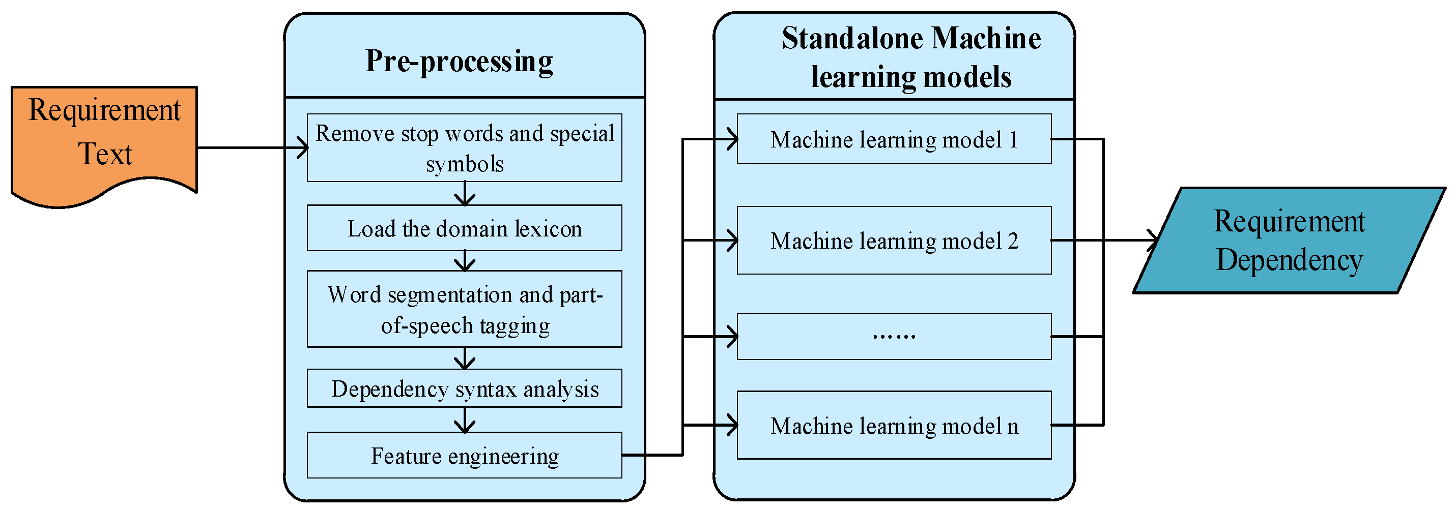
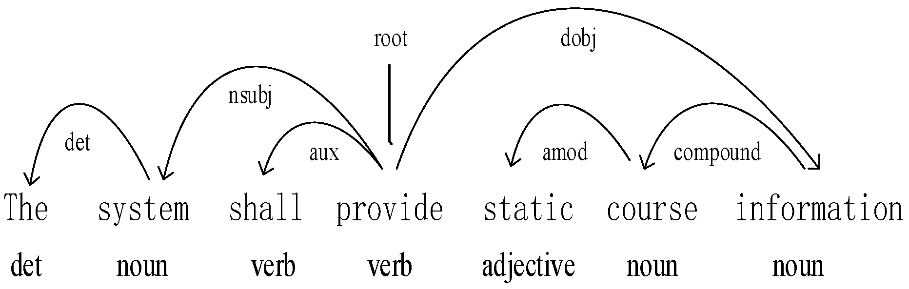
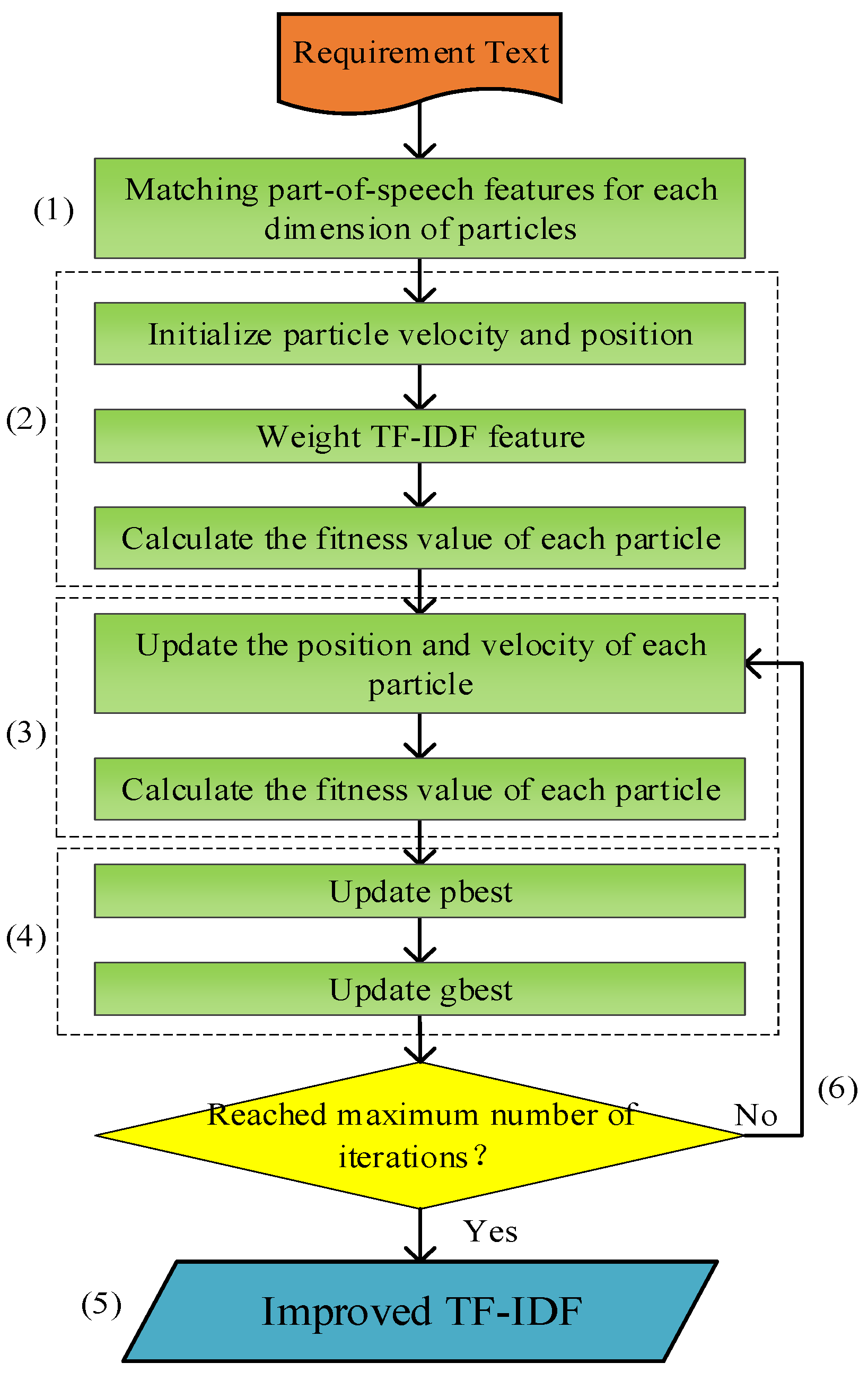
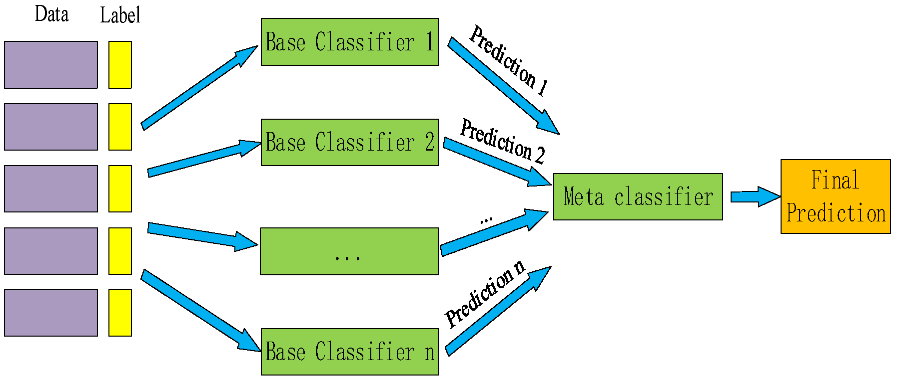
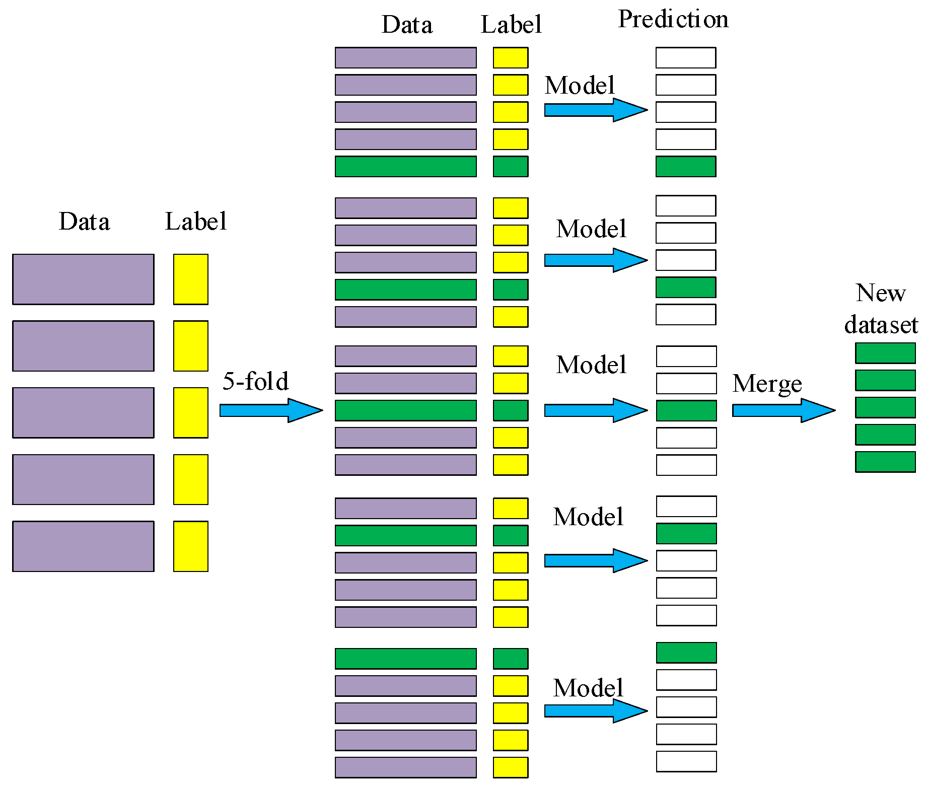
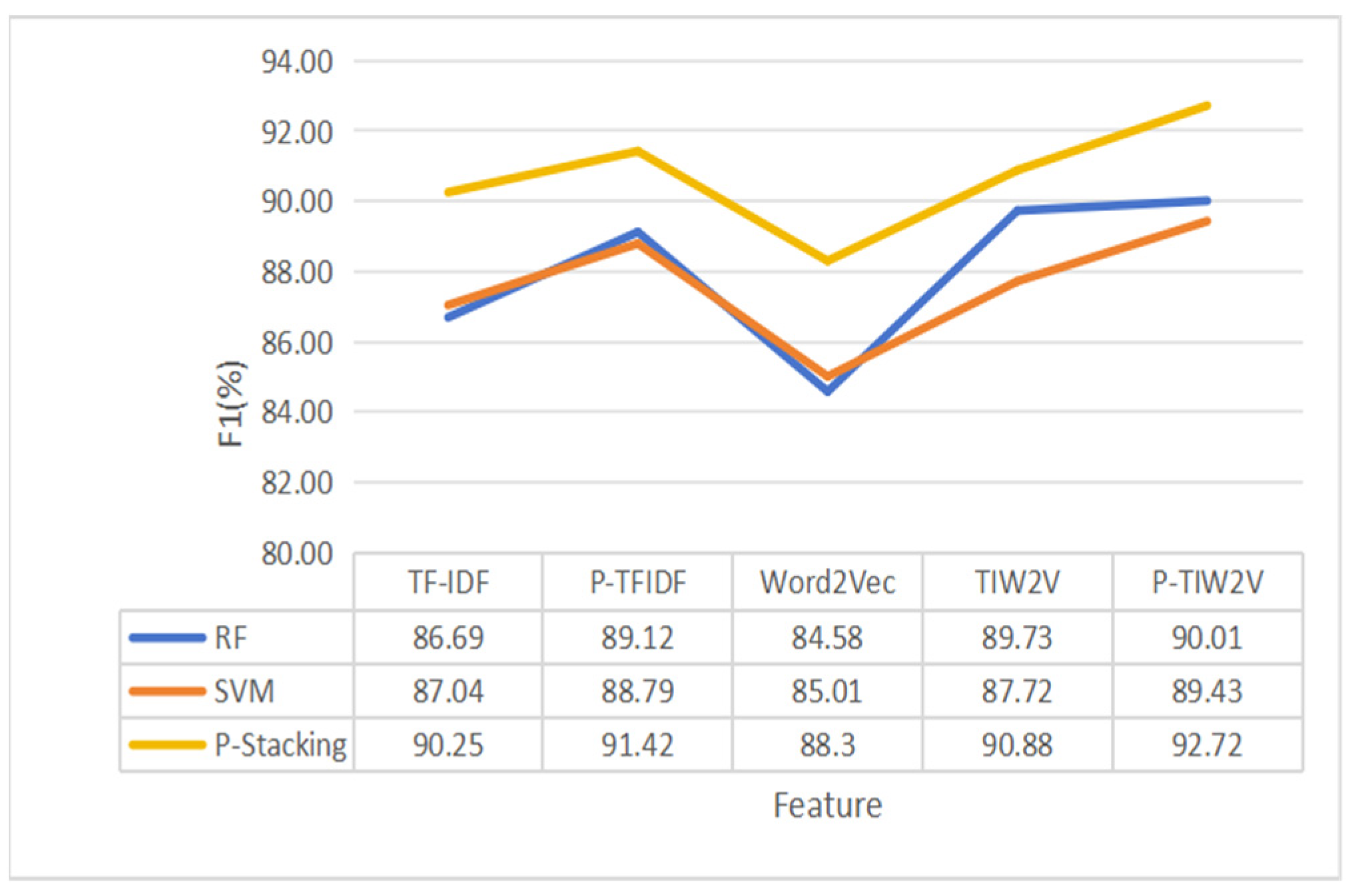
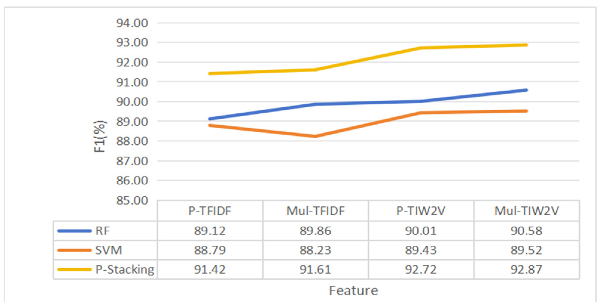
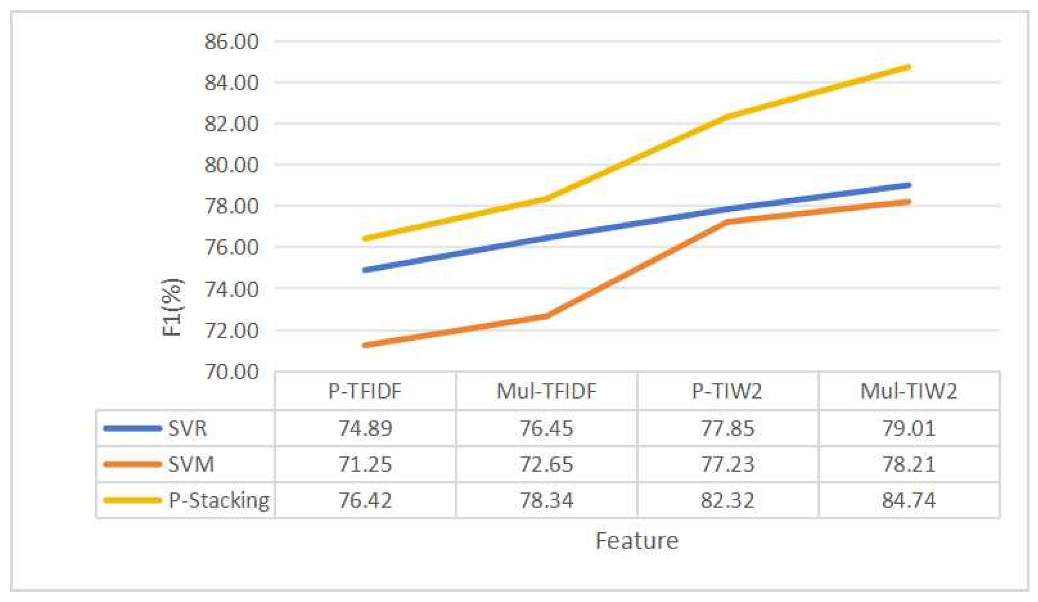
Table 1.
The feature vectors for different features.
| FEATURE | FEATURE VECTOR |
|---|---|
| TF-IDF | {0.96, 0.52, 1.08, 0.66, 0.84, 0.42, 0.64, 0.28, 1.04, 0.68, 0.94, 0.46} |
| IMPROVED TF-IDF | {1.32, 0.52, 1.48, 0.66, 1.24, 0.42, 0.85, 0.28, 1.36, 0.68, 1.23, 0.46} |
| WORD2VEC | {0.18, 0.31, 0.27, −0.23, 0.51, −0.05,0.14, −0.93, 0.34, −0.24, 0.53, 0.00} |
| TF-IDF*WORD2VEC | {0.17, 0.16, 0.29, −0.15, 0.43, −0.02, 0.09, −0.26, 0.35, −0.16, 0.50, 0.00} |
| IMPROVED TF-IDF *WORD2VEC | {0.24, 0.16, 0.41, −0.15, 0.63, −0.02, 0.12, −0.26, 0.46, −0.18, 0.65, 0.00} |
Table 2.
Part-of-speech weights in datasets with different dependency types.
| Group | Dependency Type | Part-of-Speech Weight |
|---|---|---|
| W0 | Independency | {0.24, 0.50, 0.12, 0.58, 0.22, 0.34} |
| W1 | Notification | {0.44, 0.28, 0.40, 0.18, 0.32, 0.38} |
| W2 | Arouse | {0.36, 0.26, 0.46, 0.22, 0.40, 0.30} |
| W3 | Call | {0.42, 0.60, 0.14, 0.20, 0.34, 0.30} |
| W4 | Conflict | {0.38, 0.36, 0.47, 0.32, 0.31, 0.28} |
| W5 | Aggregation | {0.48, 0.32, 0.28, 0.38, 0.20, 0.34} |
| W6 | Similar | {0.32, 0.50, 0.22, 0.34, 0.46, 0.16} |
Table 3.
The feature vectors of different features when the part-of-speech weight is W0.
| FEATURE | FEATURE VECTOR |
|---|---|
| IMPROVED TF-IDF | {1.19, 0.52, 1.62, 0.66, 0.94, 0.42, 1.01, 0.28, 1.27, 0.68, 1.26, 0.46} |
| IMPROVED TF-IDF *WORD2VEC | {0.22, 0.17, 0.44, −0.15, 0.48, −0.01, 0.12, −0.26, 0.58, −0.17, 0.82, 0.00} |
Table 4.
The feature vectors of different features when the part-of-speech weight is W1.
| FEATURE | FEATURE VECTOR |
|---|---|
| IMPROVED TF-IDF | {1.38, 0.52, 1.31, 0.66, 1.36, 0.42, 1.15, 0.28, 1.42, 0.68, 1.27, 0.46} |
| IMPROVED TF-IDF *WORD2VEC | {0.25, 0.17, 0.35, −0.15, 0.69, −0.01, 0.16, −0.26, 0.48, −0.17, 0.67, 0.00} |
Table 5.
The feature vectors of different features when the part-of-speech weight is W2.
| FEATURE | FEATURE VECTOR |
|---|---|
| IMPROVED TF-IDF | {1.38, 0.52, 1.36, 0.66, 1.73, 0.42, 1.15, 0.28, 1.42, 0.68, 1.27, 0.46} |
| IMPROVED TF-IDF *WORD2VEC | {0.25, 0.17, 0.37, −0.15, 0.88, −0.01, 0.16, −0.26, 0.68, −0.17, 0.67, 0.00} |
Table 6.
The feature vectors of different features when the part-of-speech weight is W3.
| FEATURE | FEATURE VECTOR |
|---|---|
| IMPROVED TF-IDF | {1.18, 0.52, 1.23, 0.66, 0.96, 0.42, 1.02, 0.28,1.08, 0.68, 1.02, 0.46} |
| IMPROVED TF-IDF *WORD2VEC | {0.21, 0.17, 0.33, −0.15, 0.49, −0.01, 0.14, −0.26, 0.37, −0.17, 0.54, 0.00} |
Table 7.
The feature vectors of different features when the part-of-speech weight is W4.
| FEATURE | FEATURE VECTOR |
|---|---|
| IMPROVED TF-IDF | {1.32, 0.52, 1.48, 0.66, 1.24, 0.42, 0.85, 0.28, 1.36, 0.68, 1.23, 0.46} |
| IMPROVED TF-IDF *WORD2VEC | {0.24, 0.16, 0.41, −0.15, 0.63, −0.02, 0.12, −0.26, 0.46, −0.16, 0.65, 0.00} |
Table 8.
The feature vectors of different features when the part-of-speech weight is W5.
| FEATURE | FEATURE VECTOR |
|---|---|
| IMPROVED TF-IDF | {1.37, 0.52, 1.46, 0.66, 1.39, 0.42, 1.58, 0.28, 1.23, 0.68, 1.52, 0.46} |
| IMPROVED TF-IDF *WORD2VEC | {0.25, 0.17, 0.39, −0.15, 0.71, −0.01, 0.22, −0.26, 0.42, −0.17, 0.81, 0.00} |
Table 9.
The feature vectors of different features when the part-of-speech weight is W6.
| FEATURE | FEATURE VECTOR |
|---|---|
| IMPROVED TF-IDF | {1.30, 0.52, 1.22, 0.66, 1.22, 0.42, 1.37, 0.28,1.26, 0.68, 1.09, 0.46} |
| IMPROVED TF-IDF *WORD2VEC | {0.23, 0.17, 0.33, −0.15, 0.62, −0.01, 0.19, −0.26, 0.43, −0.17, 0.58, 0.00} |
Table 10.
Experimental environment table.
| Environment | Configuration |
|---|---|
| CPU | i5-10210U |
| Random Access Memory (RAM) | 16 GB |
| Development Software | Pycharm 2020.3.5 |
| Development Language | Python 3.6 |
Table 11.
F1 values for different w, c1, and c2 values (%).
| C1 | C2 | W | FITNESS VALUE F1 (DATASET 1) | FITNESS VALUE F1 (DATASET 2) | FITNESS VALUE F1 (DATASET 3) |
|---|---|---|---|---|---|
| 2.0 | 1.0 | 0.4 | 88.63 | 77.45 | 68.39 |
| 0.5 | 89.02 | 78.48 | 68.78 | ||
| 0.6 | 88.66 | 77.76 | 68.43 | ||
| 0.7 | 88.35 | 77.62 | 68.16 | ||
| 0.8 | 88.59 | 77.63 | 67.92 | ||
| 0.9 | 88.75 | 78.15 | 68.01 | ||
| 2.0 | 2.0 | 0.4 | 88.72 | 77.60 | 68.61 |
| 0.5 | 89.24 | 78.71 | 68.93 | ||
| 0.6 | 88.81 | 77.83 | 68.54 | ||
| 0.7 | 88.59 | 77.65 | 68.28 | ||
| 0.8 | 88.69 | 77.69 | 67.99 | ||
| 0.9 | 88.76 | 78.36 | 68.12 |
Table 12.
PSO parameter values.
| Parameter | Value |
|---|---|
| c1 | 2.0 |
| c2 | 2.0 |
| w | 0.5 |
| particle number | 50 |
| iterations | 30 |
| Vmax | −0.1, +0.1 |
Table 13.
Part-of-speech weights for the three datasets.
| Datasets | Part-of-Speech Weights |
|---|---|
| Dataset 1 | {0.38, 0.36, 0.47, 0.32, 0.31, 0.28} |
| Dataset 2 | {0.47, 0.53, 0.37, 0.44, 0.72, 0.25} |
| Dataset 3 | {0.49, 0.31, 0.41, 0.55, 0.69, 0.32} |
Table 14.
F1 scores (%) for each classifier on dataset 1 at different features.
| Classifier | TF-IDF | P-TFIDF | WORD2VEC | TIW2V | P-TIW2V |
|---|---|---|---|---|---|
| KNN | 65.98 | 73.67 | 69.12 | 68.55 | 75.37 |
| DT | 83.42 | 88.02 | 81.45 | 89.28 | 89.45 |
| LGR | 81.27 | 85.38 | 80.73 | 84.03 | 87.62 |
| RF | 86.69 | 89.12 | 84.58 | 89.73 | 90.01 |
| SVM | 87.04 | 88.79 | 85.01 | 87.72 | 89.43 |
| GNB | 57.64 | 63.95 | 70.64 | 71.5 | 72.27 |
| MNB | 70.1 | 71.53 | 70.63 | 68.6 | 74.56 |
| SVR | 83.72 | 85.2 | 80.67 | 85.23 | 87.06 |
| LR | 81.96 | 83.24 | 80.33 | 82.47 | 85.24 |
Table 15.
F1 scores (%) for each classifier on dataset 2 at different features.
| Classifier | TF-IDF | P-TFIDF | WORD2VEC | TIW2V | P-TIW2V |
|---|---|---|---|---|---|
| KNN | 52.05 | 55.39 | 59.53 | 61.12 | 63.74 |
| DT | 71.23 | 72.68 | 68.9 | 72.63 | 75.12 |
| LGR | 61.85 | 63.14 | 54.21 | 58.84 | 64.98 |
| RF | 72.26 | 78.65 | 80.53 | 80.75 | 82.69 |
| SVM | 70.49 | 73.9 | 67.99 | 68.85 | 73.27 |
| GNB | 45.25 | 48.08 | 49.53 | 51.62 | 52.3 |
| MNB | 54.07 | 55.47 | 41.84 | 43.54 | 47.28 |
| SVR | 60.67 | 68.93 | 64.32 | 69.06 | 74.58 |
| LR | 62.35 | 65.41 | 53.89 | 60.58 | 65.9 |
Table 16.
F1 scores (%) for each classifier on dataset 3 at different features.
| Classifier | TF-IDF | P-TFIDF | WORD2VEC | TIW2V | P-TIW2V |
|---|---|---|---|---|---|
| KNN | 42.24 | 50.19 | 64.57 | 69.46 | 75.87 |
| DT | 62.9 | 67.06 | 73.82 | 73.08 | 78.29 |
| LGR | 66.44 | 68.27 | 63.65 | 69.25 | 70.48 |
| RF | 59.75 | 69.36 | 75.4 | 77.98 | 79.06 |
| SVM | 70.03 | 71.25 | 69.0 | 74.52 | 77.23 |
| GNB | 30.7 | 38.59 | 59.1 | 58.45 | 60.27 |
| MNB | 58.48 | 60.27 | 27.99 | 30.34 | 30.6 |
| SVR | 72.38 | 74.89 | 71.26 | 74.78 | 77.85 |
| LR | 67.45 | 72.04 | 65.86 | 70.67 | 74.61 |
Table 17.
Precision and Recall values (%) for each classifier on dataset 1 at different features.
| TF-IDF | P-TFIDF | WORD2VEC | TIW2V | P-TIW2V | ||||||
|---|---|---|---|---|---|---|---|---|---|---|
| Classifier | Recall | Precision | Recall | Precision | Recall | Precision | Recall | Precision | Recall | Precision |
| KNN | 64.45 | 67.44 | 72.96 | 74.28 | 70.41 | 67.76 | 67.95 | 69.02 | 74.21 | 76.56 |
| DT | 85.14 | 81.63 | 87.25 | 88.91 | 82.69 | 80.14 | 87.26 | 91.28 | 89.32 | 89.57 |
| LGR | 81.25 | 81.17 | 85.23 | 85.47 | 79.57 | 81.84 | 84.25 | 83.74 | 88.56 | 86.62 |
| RF | 86.24 | 87.02 | 89.96 | 88.16 | 83.15 | 86.25 | 89.67 | 89.80 | 87.45 | 92.70 |
| SVM | 88.17 | 85.75 | 87.45 | 90.03 | 84.04 | 86.09 | 86.14 | 89.46 | 90.32 | 88.55 |
| GNB | 54.93 | 61.04 | 64.57 | 63.25 | 72.94 | 68.36 | 73.47 | 69.53 | 71.14 | 73.43 |
| MNB | 69.14 | 71.16 | 71.69 | 71.28 | 73.45 | 68.14 | 69.32 | 67.91 | 74.52 | 74.64 |
| SVR | 84.68 | 82.67 | 86.47 | 83.84 | 78.36 | 83.16 | 85.27 | 85.21 | 84.47 | 89.83 |
| LR | 82.35 | 81.63 | 82.74 | 83.62 | 80.99 | 79.66 | 83.96 | 81.34 | 86.36 | 84.14 |
Table 18.
Precision and Recall values (%) for each classifier on dataset 2 at different features.
| TF-IDF | P-TFIDF | WORD2VEC | TIW2V | P-TIW2V | ||||||
|---|---|---|---|---|---|---|---|---|---|---|
| Classifier | Recall | Precision | Recall | Precision | Recall | Precision | Recall | Precision | Recall | Precision |
| KNN | 51.32 | 52.74 | 55.27 | 55.46 | 56.18 | 63.32 | 64.64 | 57.81 | 64.58 | 62.86 |
| DT | 72.84 | 69.58 | 76.14 | 69.47 | 69.32 | 68.54 | 71.85 | 73.52 | 74.65 | 75.51 |
| LGR | 62.95 | 60.65 | 64.25 | 62.14 | 55.20 | 53.24 | 56.29 | 61.74 | 65.21 | 64.68 |
| RF | 72.41 | 72.23 | 77.56 | 79.68 | 81.94 | 79.26 | 81.96 | 79.40 | 80.14 | 85.36 |
| SVM | 71.46 | 69.61 | 73.36 | 74.59 | 66.57 | 69.38 | 67.31 | 70.51 | 74.54 | 72.16 |
| GNB | 47.12 | 43.65 | 49.70 | 46.63 | 48.26 | 50.63 | 50.62 | 52.67 | 54.26 | 50.56 |
| MNB | 53.73 | 54.32 | 56.31 | 54.74 | 42.61 | 41.25 | 44.68 | 42.49 | 45.96 | 48.72 |
| SVR | 61.87 | 59.64 | 69.83 | 68.14 | 65.85 | 62.77 | 69.67 | 68.56 | 78.36 | 71.06 |
| LR | 63.65 | 61.18 | 66.37 | 64.52 | 52.65 | 55.21 | 61.37 | 59.72 | 66.03 | 65.79 |
Table 19.
Precision and Recall values (%) for each classifier on dataset 3 at different features.
| TF-IDF | P-TFIDF | WORD2VEC | TIW2V | P-TIW2V | ||||||
|---|---|---|---|---|---|---|---|---|---|---|
| Classifier | Recall | Precision | Recall | Precision | Recall | Precision | Recall | Precision | Recall | Precision |
| KNN | 45.97 | 39.15 | 54.87 | 46.14 | 66.67 | 62.38 | 68.63 | 70.22 | 76.96 | 74.65 |
| DT | 63.46 | 62.47 | 66.12 | 68.25 | 72.91 | 74.56 | 70.46 | 75.81 | 75.64 | 81.03 |
| LGR | 65.32 | 67.52 | 70.58 | 66.03 | 60.53 | 67.04 | 71.96 | 66.76 | 71.36 | 69.12 |
| RF | 59.47 | 60.07 | 74.67 | 64.86 | 76.55 | 74.16 | 75.67 | 80.32 | 78.48 | 79.68 |
| SVM | 71.65 | 68.30 | 70.35 | 72.03 | 71.96 | 66.30 | 72.67 | 76.42 | 76.34 | 78.06 |
| GNB | 27.01 | 35.46 | 34.52 | 43.66 | 62.01 | 56.36 | 56.65 | 60.25 | 64.26 | 56.68 |
| MNB | 56.31 | 60.75 | 59.41 | 61.04 | 25.36 | 31.24 | 36.39 | 26.10 | 35.49 | 26.76 |
| SVR | 75.64 | 69.42 | 76.36 | 73.36 | 74.36 | 68.31 | 72.68 | 77.06 | 78.52 | 77.23 |
| LR | 68.17 | 66.87 | 72.68 | 71.50 | 60.89 | 71.72 | 74.13 | 67.65 | 75.64 | 73.54 |
Table 20.
Precision and Recall values (%) for P-Stacking on three datasets at different features.
| TF-IDF | P-TFIDF | Word2vec | TIW2V | P-TIW2V | ||||||
|---|---|---|---|---|---|---|---|---|---|---|
| Datasets | Recall | Precision | Recall | Precision | Recall | Precision | Recall | Precision | Recall | Precision |
| Dataset 1 | 89.47 | 91.13 | 92.64 | 90.14 | 89.17 | 87.38 | 89.27 | 92.49 | 93.65 | 91.79 |
| Dataset 2 | 85.21 | 81.69 | 84.60 | 86.84 | 84.91 | 80.32 | 87.46 | 82.79 | 85.73 | 89.75 |
| Dataset 3 | 76.58 | 72.13 | 74.28 | 78.59 | 75.34 | 78.21 | 78.62 | 79.42 | 81.09 | 83.64 |
Table 21.
Part-of-speech weights in dataset 1 with different dependency types.
| Group | Dependency Type | Part-of-Speech Weights |
|---|---|---|
| W0 | Independency | {0.24, 0.50, 0.12, 0.58, 0.22, 0.34} |
| W1 | Notification | {0.44, 0.28, 0.40, 0.18, 0.32, 0.38} |
| W2 | Arouse | {0.36, 0.26, 0.46, 0.22, 0.40, 0.30} |
| W3 | Call | {0.42, 0.60, 0.14, 0.20, 0.34, 0.30} |
| W4 | Conflict | {0.38, 0.36, 0.47, 0.32, 0.31, 0.28} |
| W5 | Aggregation | {0.48, 0.32, 0.28, 0.38, 0.20, 0.34} |
| W6 | Similar | {0.32, 0.50, 0.22, 0.34, 0.46, 0.16} |
Table 22.
Part-of-speech weights in dataset 2 with different dependency types.
| Group | Dependency Type | Part-of-Speech Weights |
|---|---|---|
| W0 | Independency | {0.38, 0.25, 0.22, 0.36, 0.56, 0.35} |
| W1 | Notification | {0.45, 0.53, 0.52, 0.75, 0.26, 0.70} |
| W2 | Arouse | {0.52, 0.63, 0.55, 0.51, 0.79, 0.51} |
| W3 | Call | {0.65, 0.30, 0.45, 0.39, 0.64, 0.26} |
| W4 | Conflict | {0.50, 0.23, 0.75, 0.31, 0.74, 0.64} |
Table 23.
Part-of-speech weights in dataset 3 with different dependency types.
| Group | Dependency Type | Part-of-Speech Weights |
|---|---|---|
| W0 | Independency | {0.37, 0.22, 0.32, 0.41, 0.65, 0.43} |
| W1 | Notification | {0.56, 0.55, 0.76, 0.44, 0.67, 0.35} |
| W2 | Arouse | {0.43, 0.36, 0.33, 0.53, 0.77, 0.55} |
| W3 | Call | {0.39, 0.25, 0.35, 0.73, 0.41, 0,37} |
| W5 | Aggregation | {0.74, 0.40, 0.35, 0.36, 0.63, 0.37} |
| W6 | Similar | {0.29, 0.42, 0.69, 0.24, 0.70, 0.28} |
Table 24.
F1 scores (%) for each classifier on the Course Management System dataset at different features.
Table 24.
F1 scores (%) for each classifier on the Course Management System dataset at different features.
| Classifier | P-TFIDF | MUL-TFIDF | P-TIW2V | MUL-TIW2V |
|---|---|---|---|---|
| KNN | 73.67 | 73.52 | 75.37 | 75.36 |
| DT | 88.02 | 88.65 | 89.45 | 89.76 |
| LGR | 85.38 | 86.02 | 87.62 | 88.34 |
| RF | 89.12 | 89.86 | 90.01 | 90.58 |
| SVM | 88.79 | 88.23 | 89.43 | 89.52 |
| GNB | 63.95 | 63.25 | 72.27 | 73.22 |
| MNB | 71.53 | 72.65 | 74.56 | 74.89 |
| SVR | 85.2 | 85.36 | 87.06 | 87.41 |
| LR | 83.24 | 83.41 | 85.24 | 86.23 |
Table 25.
F1 scores (%) for each classifier on the Composition Evaluation dataset at different features.
Table 25.
F1 scores (%) for each classifier on the Composition Evaluation dataset at different features.
| Classifier | P-TFIDF | MUL-TFIDF | P-TIW2V | MUL-TIW2V |
|---|---|---|---|---|
| KNN | 55.39 | 56.03 | 63.74 | 64.20 |
| DT | 72.68 | 72.79 | 75.12 | 75.26 |
| LGR | 63.14 | 63.17 | 64.98 | 66.31 |
| RF | 78.65 | 78.52 | 82.69 | 82.94 |
| SVM | 73.9 | 75.23 | 73.27 | 74.14 |
| GNB | 48.08 | 48.57 | 52.3 | 53.03 |
| MNB | 55.47 | 55.36 | 47.28 | 47.25 |
| SVR | 68.93 | 69.01 | 74.58 | 74.69 |
| LR | 65.41 | 66.74 | 65.9 | 67.21 |
Table 26.
F1 scores (%) for each classifier on the CMS System dataset at different features.
| Classifier | P-TFIDF | MUL-TFIDF | P-TIW2V | MUL-TIW2V |
|---|---|---|---|---|
| KNN | 50.19 | 50.63 | 75.87 | 76.41 |
| DT | 67.06 | 68.62 | 78.29 | 80.16 |
| LGR | 68.27 | 69.20 | 70.48 | 71.54 |
| RF | 69.36 | 71.53 | 79.06 | 80.32 |
| SVM | 71.25 | 72.65 | 77.23 | 78.21 |
| GNB | 38.59 | 40.23 | 60.27 | 61.03 |
| MNB | 60.27 | 61.94 | 30.6 | 35.26 |
| SVR | 74.89 | 76.45 | 77.85 | 79.01 |
| LR | 72.04 | 74.64 | 74.61 | 75.36 |
Table 27.
Precision and Recall values (%) for each classifier on dataset 1 at different features.
| P-TFIDF | MUL-TFIDF | P-TIW2V | MUL-TIW2V | |||||
|---|---|---|---|---|---|---|---|---|
| Classifier | Recall | Precision | Recall | Precision | Recall | Precision | Recall | Precision |
| KNN | 72.96 | 74.28 | 74.56 | 72.61 | 74.21 | 76.56 | 74.26 | 76.33 |
| DT | 87.25 | 88.91 | 88.66 | 88.57 | 89.32 | 89.57 | 89.64 | 89.96 |
| LGR | 85.23 | 85.47 | 87.41 | 84.63 | 88.56 | 86.62 | 86.47 | 90.32 |
| RF | 89.96 | 88.16 | 88.94 | 90.96 | 87.45 | 90.24 | 90.83 | 92.70 |
| SVM | 87.45 | 90.03 | 89.64 | 86.72 | 90.32 | 88.55 | 88.87 | 90.07 |
| GNB | 64.57 | 63.25 | 65.41 | 61.38 | 71.14 | 73.43 | 74.51 | 71.86 |
| MNB | 71.69 | 71.28 | 70.54 | 74.76 | 74.52 | 74.64 | 73.17 | 76.55 |
| SVR | 86.47 | 83.84 | 85.77 | 84.82 | 84.47 | 89.83 | 88.69 | 86.07 |
| LR | 82.74 | 83.62 | 83.56 | 83.25 | 86.36 | 84.14 | 88.69 | 85.89 |
Table 28.
Precision and Recall values (%) for each classifier on dataset 2 at different features.
| P-TFIDF | MUL-TFIDF | P-TIW2V | MUL-TIW2V | |||||
|---|---|---|---|---|---|---|---|---|
| Classifier | Recall | Precision | Recall | Precision | Recall | Precision | Recall | Precision |
| KNN | 55.27 | 55.46 | 55.78 | 56.14 | 64.58 | 62.86 | 63.58 | 64.67 |
| DT | 76.14 | 69.47 | 71.03 | 74.58 | 74.65 | 75.51 | 77.64 | 73.16 |
| LGR | 64.25 | 62.14 | 64.26 | 62.14 | 65.21 | 64.68 | 68.43 | 64.36 |
| RF | 77.56 | 79.68 | 77.29 | 79.66 | 80.14 | 85.36 | 81.06 | 84.89 |
| SVM | 73.36 | 74.59 | 73.65 | 76.78 | 74.54 | 72.16 | 72.87 | 75.49 |
| GNB | 49.70 | 46.63 | 46.98 | 50.16 | 54.26 | 50.56 | 54.39 | 51.86 |
| MNB | 56.31 | 54.74 | 58.47 | 52.54 | 45.96 | 48.72 | 49.61 | 45.25 |
| SVR | 69.83 | 68.14 | 70.14 | 67.85 | 78.36 | 71.06 | 75.67 | 73.65 |
| LR | 66.37 | 64.52 | 65.39 | 68.20 | 66.03 | 65.79 | 68.59 | 65.79 |
Table 29.
Precision and Recall values (%) for each classifier on dataset 3 at different features.
| P-TFIDF | MUL-TFIDF | P-TIW2V | MUL-TIW2V | |||||
|---|---|---|---|---|---|---|---|---|
| Classifier | Recall | Precision | Recall | Precision | Recall | Precision | Recall | Precision |
| KNN | 54.87 | 46.14 | 51.94 | 49.24 | 76.96 | 74.65 | 77.42 | 75.26 |
| DT | 66.12 | 68.25 | 66.67 | 70.51 | 75.64 | 81.03 | 81.67 | 78.68 |
| LGR | 70.58 | 66.03 | 70.25 | 68.24 | 71.36 | 69.12 | 70.69 | 72.34 |
| RF | 74.67 | 64.86 | 70.43 | 72.61 | 78.48 | 79.68 | 82.49 | 78.32 |
| SVM | 70.35 | 72.03 | 74.56 | 70.69 | 76.34 | 78.06 | 76.85 | 79.64 |
| GNB | 34.52 | 43.66 | 45.97 | 35.69 | 64.26 | 56.68 | 63.56 | 58.57 |
| MNB | 59.41 | 61.04 | 63.04 | 60.91 | 35.49 | 26.76 | 38.15 | 32.65 |
| SVR | 76.36 | 73.36 | 78.13 | 74.68 | 78.52 | 77.23 | 76.49 | 81.65 |
| LR | 72.68 | 71.50 | 75.96 | 73.25 | 75.64 | 73.54 | 77.25 | 73.58 |
Table 30.
Precision and Recall values (%) for P-Stacking on three datasets using different features.
Table 30.
Precision and Recall values (%) for P-Stacking on three datasets using different features.
| P-TFIDF | TIW2V | P-TIW2V | Mul-TFIDF | |||||
|---|---|---|---|---|---|---|---|---|
| Dataset | Recall | Precision | Recall | Precision | Recall | Precision | Recall | Precision |
| Dataset 1 | 90.56 | 92.18 | 92.14 | 91.16 | 91.86 | 93.47 | 93.01 | 92.61 |
| Dataset 2 | 83.29 | 88.36 | 86.64 | 85.17 | 85.62 | 89.93 | 89.30 | 86.75 |
| Dataset 3 | 73.61 | 79.39 | 80.59 | 76.10 | 84.17 | 80.36 | 80.26 | 89.53 |
Table 31.
The F1, Recall, and Precision (%) values of different requirement sentence backbone extraction methods on each classifier.
Table 31.
The F1, Recall, and Precision (%) values of different requirement sentence backbone extraction methods on each classifier.
| OE | PE | |||||
|---|---|---|---|---|---|---|
| Classifier | Recall | Precision | F1 | Recall | Precision | F1 |
| KNN | 77.42 | 75.26 | 76.41 | 75.24 | 79.64 | 77.42 |
| DT | 81.67 | 78.68 | 80.16 | 82.04 | 80.11 | 80.98 |
| LGR | 70.69 | 72.34 | 71.54 | 76.35 | 72.18 | 74.25 |
| RF | 82.49 | 78.32 | 80.32 | 80.26 | 83.09 | 81.69 |
| SVM | 76.85 | 79.64 | 78.21 | 78.94 | 79.36 | 79.18 |
| GNB | 63.56 | 58.57 | 61.03 | 68.36 | 63.89 | 66.03 |
| MNB | 38.15 | 32.65 | 35.26 | 41.29 | 37.86 | 39.46 |
| SVR | 76.49 | 81.65 | 79.01 | 82.67 | 78.25 | 80.34 |
| LR | 77.25 | 73.58 | 75.36 | 78.39 | 75.97 | 77.12 |
| P-Stacking | 80.26 | 89.53 | 84.74 | 88.57 | 84.39 | 86.48 |
Table 32.
Program run time (s) for three datasets.
| Datasets | Time 1 | Time 2 | Time 3 | Time 4 | Sum |
|---|---|---|---|---|---|
| Dataset 1 | 136.2554 | 1.6974 | 4.1350 | 11.4882 | 153.5760 |
| Dataset 2 | 124.6930 | 1.2841 | 5.0362 | 14.0194 | 145.0327 |
| Dataset 3 | 150.2494 | 1.3758 | 3.7022 | 14.9853 | 170.3127 |
Table 33.
The nine models of program run time (s) in dataset 1.
| Classifier | Train | Test |
|---|---|---|
| KNN | 0.1324 | 0.0102 |
| DT | 0.1631 | 0.0214 |
| LGR | 0.1009 | 0.0165 |
| RF | 0.1660 | 0.0222 |
| SVM | 0.0506 | 0.0166 |
| GNB | 0.0796 | 0.0060 |
| MNB | 0.2305 | 0.0997 |
| SVR | 0.1829 | 0.0172 |
| LR | 0.0714 | 0.0065 |
Table 34.
The nine models of program run time (s) in dataset 2.
| Classifier | Train | Test |
|---|---|---|
| KNN | 0.1694 | 0.0152 |
| DT | 0.0823 | 0.0251 |
| LGR | 0.1728 | 0.0365 |
| RF | 0.1166 | 0.0329 |
| SVM | 0.1674 | 0.0270 |
| GNB | 0.0515 | 0.0041 |
| MNB | 0.1002 | 0.0094 |
| SVR | 0.1497 | 0.0213 |
| LR | 0.0879 | 0.0012 |
Table 35.
The nine models of program run time (s) in dataset 3.
| Classifier | Train | Test |
|---|---|---|
| KNN | 0.1042 | 0.0099 |
| DT | 0.0641 | 0.0236 |
| LGR | 0.0159 | 0.0140 |
| RF | 0.1249 | 0.0156 |
| SVM | 0.0412 | 0.0187 |
| GNB | 0.0213 | 0.0045 |
| MNB | 0.1746 | 0.0540 |
| SVR | 0.1714 | 0.0074 |
| LR | 0.0616 | 0.0168 |
Table 36.
Three deep learning models of program run time (s) and F1 (%) in the three datasets.
| Datasets | Deep Learning | Epochs | Time | RECALL | PRECISION | F1 |
|---|---|---|---|---|---|---|
| DATASET 1 | LSTM | 30 | 60.3233 | 69.51 | 56.96 | 62.45 |
| Bi-LSTM | 30 | 68.9160 | 57.31 | 37.09 | 45.03 | |
| CNN | 30 | 35.6623 | 51.22 | 39.56 | 38.40 | |
| DATASET 2 | LSTM | 30 | 54.3155 | 52.42 | 39.80 | 45.12 |
| Bi-LSTM | 30 | 70.6251 | 58.25 | 52.49 | 53.63 | |
| CNN | 30 | 40.2136 | 55.33 | 42.98 | 47.56 | |
| DATASET 3 | LSTM | 30 | 64.3598 | 56.39 | 47.13 | 39.80 |
| Bi-LSTM | 30 | 75.1466 | 57.34 | 44.94 | 48.79 | |
| CNN | 30 | 50.1220 | 44.61 | 52.13 | 45.54 |
Disclaimer/Publisher’s Note: The statements, opinions and data contained in all publications are solely those of the individual author(s) and contributor(s) and not of MDPI and/or the editor(s). MDPI and/or the editor(s) disclaim responsibility for any injury to people or property resulting from any ideas, methods, instructions or products referred to in the content. |
© 2024 by the authors. Licensee MDPI, Basel, Switzerland. This article is an open access article distributed under the terms and conditions of the Creative Commons Attribution (CC BY) license (https://creativecommons.org/licenses/by/4.0/).
Share and Cite
MDPI and ACS Style
Guan, H.; Xu, H.; Cai, L. Requirement Dependency Extraction Based on Improved Stacking Ensemble Machine Learning. Mathematics 2024, 12, 1272. https://doi.org/10.3390/math12091272
AMA Style
Guan H, Xu H, Cai L. Requirement Dependency Extraction Based on Improved Stacking Ensemble Machine Learning. Mathematics. 2024; 12(9):1272. https://doi.org/10.3390/math12091272
Chicago/Turabian StyleGuan, Hui, Hang Xu, and Lie Cai. 2024. "Requirement Dependency Extraction Based on Improved Stacking Ensemble Machine Learning" Mathematics 12, no. 9: 1272. https://doi.org/10.3390/math12091272
Note that from the first issue of 2016, this journal uses article numbers instead of page numbers. See further details here.