Synergising an Advanced Optimisation Technique with Deep Learning: A Novel Method in Fault Warning Systems

Abstract

In the realm of automated industry and smart production, the deployment of fault warning systems is crucial for ensuring equipment reliability and enhancing operational efficiency. Although there are a multitude of existing methodologies for fault warning, the proficiency of these systems in processing and analysing data is increasingly challenged by the progression of industrial apparatus and the escalating magnitude and intricacy of the data involved. To address these challenges, this research outlines an innovative fault warning methodology that combines a bi-directional long short-term memory (Bi-LSTM) network with an enhanced hunter–prey optimisation (EHPO) algorithm. The Bi-LSTM network is strategically utilised to outline complex temporal patterns in machinery operational data, while the EHPO algorithm is employed to meticulously fine-tune the hyperparameters of the Bi-LSTM, aiming to enhance the accuracy and generalisability of fault warning. The EHPO algorithm, building upon the foundational hunter–prey optimisation (HPO) framework, introduces an advanced population initialisation process, integrates a range of strategic exploration methodologies, and strengthens its search paradigms through the incorporation of the differential evolution (DE) algorithm. This comprehensive enhancement aims to boost the global search efficiency and accelerate the convergence speed of the algorithm. Empirical analyses, conducted using datasets from real-world industrial scenarios, have validated the improved warning performance of this proposed methodology against some benchmark techniques, as evidenced by superior metrics such as root mean square error (RMSE) and mean absolute error (MAE), albeit with a slight increase in computational resource requirements. This study not only proposes a novel paradigm for fault warning within complex industrial frameworks but also contributes to the discourse on hyperparameter optimisation within the field of machine learning algorithms.

1. Introduction

The concepts of automation and intelligent manufacturing have emerged as the driving force behind industrial development in the modern era [1]. As technological advancements lead to increasingly complex machinery and equipment being used on production lines, there is a growing demand for precision operation and efficiency in ever-changing production environments [2]. This complexity necessitates higher standards of reliability and stability, as any malfunction can lead to production halts, compromised product quality, and potential safety incidents [3,4]. Consequently, fault warning systems play an indispensable role in contemporary industry, enabling predictive maintenance, reducing downtime, and extending equipment lifespan [5].

Despite the escalating importance of fault warning systems, existing methods face significant challenges when dealing with large-scale, high-dimensional, and non-linear industrial data. These methods struggle to accurately detect early signs of fault development in complex time-series data, resulting in suboptimal accuracy and timeliness in the generated warnings. Moreover, with the advent of Industry 4.0, the exponential growth in data generated by this equipment further compounds the complexity of fault warning systems [6].

To address these challenges, this study proposes an innovative fault warning methodology that harnesses the strengths of deep learning and metaheuristic algorithms. We employ a Bi-LSTM network to capture complex temporal patterns in equipment and operational data. As an advanced deep learning model, the Bi-LSTM is particularly adept at handling time-series data and identifying potential fault precursors. However, the performance of the Bi-LSTM model is heavily contingent upon the tuning of its hyperparameters, a process that typically requires extensive experimentation and expert insight, making it time-consuming and costly in practice. The development of metaheuristic algorithms has paved the way to overcome this bottleneck. It is important to note the “No Free Lunch” theorem in the optimisation domain [7], which underscores the trade-off between the universality and specificity of optimisation algorithms. This theorem posits that no single algorithm can optimise all possible problems, thereby encouraging researchers to develop new algorithms and improve existing ones. In this study, we introduce an EHPO algorithm designed to overcome the limitations of traditional fault warning methods when handling complex industrial data. Inspired by the dynamic pursuit between hunters and prey in nature, the EHPO algorithm simulates this process to find optimal solutions. We incorporate an efficient population initialisation strategy and integrate multiple search techniques to enhance the algorithm’s global search capabilities and convergence speed in complex search spaces. Furthermore, we fuse the DE algorithm to further improve performance, enabling the EHPO algorithm to explore the parameter space more effectively and identify the optimal hyperparameter configuration, thereby enhancing the accuracy and generalisation of fault predictions.

Experimental results obtained using real-world industrial case datasets demonstrate the superior performance of our proposed method in fault warning, surpassing existing advanced methods in predictive accuracy and showing distinct advantages in key performance metrics such as the RMSE and MAE. Although there is an increase in computational time, considering the significance of fault warning, this investment is justified. Figure 1 shows the execution framework of the hybrid method developed in this paper.

In summary, the main research questions (RQs) of this paper are as follows:

RQ1: How does the integration of a Bi-LSTM network and an EHPO algorithm in a novel fault warning method enhance the accuracy and efficiency of fault warnings? This paper introduces this innovative approach, which leverages the strengths of deep learning in identifying complex temporal patterns and the adaptability of metaheuristic algorithms in hyperparameter optimisation.

RQ2: How does the enhancement of the HPO algorithm expand its application scope and demonstrate its potential in the field of industrial fault warning? This paper not only improves the performance of the model but also explores new possibilities for the application of HPO algorithms in other complex optimisation problems.

RQ3: How does the theoretical presentation of a new fault warning framework translate into practical application in specific industrial environments? This paper not only proposes a new method but also implements and tests it in real-world scenarios, demonstrating its applicability and effectiveness.

The remainder of this paper is organised as follows: First, we review the progress in related fields and provide an in-depth analysis (Section 2). We then introduce the core mechanisms of the EHPO algorithm and the Bi-LSTM model, as well as their integration (Section 3). Subsequently, we present the performance of the proposed method on real industrial datasets (Section 4) and compare it with other methods (Section 5). Section 6 analyses the positive impact of this paper on industry. Finally, we discuss the limitations of this study and outline future research directions (Section 7).

2. Literature Review

With the rapid development of industrial automation and intelligent manufacturing, fault warning systems are playing an increasingly important role in maintaining equipment stability and enhancing production efficiency [8,9]. These systems can monitor and analyse equipment operation data in real-time, identifying potential fault risks in advance, thereby reducing downtime and preventing production losses. Against this backdrop, researchers have proposed a variety of fault warning methods to cope with the growing complexity of industrial systems. Traditional fault warning methods, such as rule-based expert systems and frequency domain analysis, although effective in specific scenarios, face many challenges when dealing with large-scale, high-dimensional, and nonlinear industrial data. These methods often struggle to capture the complex temporal patterns in the data, leading to insufficient predictive accuracy [10]. In recent years, machine learning technologies have been widely applied in industrial fault warning. For example, Chen et al. [11] used a genetic algorithm (GA) to optimise a backpropagation (BP) neural network (GA-BP) for wind turbine pitch system fault warning. Lu et al. [12] devised a strategy for preemptive fault alerts during the charging of Electric Vehicles, grounded in the Adaptive Deep Belief Network. They applied nesterov accelerated adaptive moment estimation for the optimisation phase and constructed an adaptive deep belief network model representing the standard EV charging process, utilising historical EV charging data. This approach delivered accurate, real-time fault forecasting, providing robust technical assistance for EV charging fault alerts. Li et al. [13] focused on subtle, inter-turn, short-circuit faults in synchronous generators’ excitation windings and introduced an innovative warning technique. They employed an advanced particle swarm optimisation (PSO) algorithm to define the gated recurrent unit—the convolutional neural network model’s structural parameters—and used the total deviation distance as the fault detection metric. Their approach was empirically verified, charting a fresh path for synchronous generator fault diagnosis. Jing et al. [14] put forward a microservice fault detection strategy based on a light gradient boosting machine (LightGBM). By scrutinising historical operational data, they ensured high reliability, presenting a novel approach to microservice fault detection. Sun et al. [15] proposed a vibration prediction model that integrates complete ensemble empirical mode decomposition with adaptive noise and long short-term memory (LSTM) neural networks. This model utilises an improved particle swarm optimisation (IPSO) algorithm to optimise the tuning parameters of the LSTM, thereby enhancing the accuracy of the predictions. Zhao et al. [16] suggested a deep learning approach, specifically a deep autoencoder network, to analyse sensor data and issue early alerts for potential faults in wind turbine components. This method introduced a novel technical approach to providing early warnings of wind turbine component faults. Chen et al. [17] employed a GA to refine the BP neural network, delivering alerts for impending faults in wind turbines’ pitch systems. This approach offered an innovative solution for pitch system fault warnings. Wang et al. [18] created an advanced deep learning model, specifically a multi-stage fusion LSTM model. They analysed the spatiotemporal characteristics of operational data to forecast future parameters of reciprocating compressor valves, thus contributing to the objective of early fault detection. This approach presented a new solution for fault warning in reciprocating compressor valves. Cai et al. [19] utilised historical data from power systems and machine learning, particularly the extreme gradient boosting algorithm (XGBoost), to devise a predictive model for power distribution network outages. This strategy facilitated early fault warnings and maintenance scheduling for distribution network issues, providing a new approach to power system fault alerts. Liu et al. [20] leveraged the grey wolf optimisation algorithm to refine the support vector regression (GWO-SVR) model for fault warnings in wind turbine gearboxes. This methodology incorporated random forest feature selection and a sliding smooth filtering process for the treatment of input data. The experimental outcomes demonstrated that the model’s warning performance was superior to several other comparative models.

Deep learning models have demonstrated their potential in the field of fault warning, but the performance of these models largely depends on the configuration of their hyperparameters. Traditional hyperparameter tuning methods, such as grid search and random search, are often inefficient, especially when dealing with vast parameter spaces. Consequently, researchers have begun to explore the use of evolutionary algorithms, such as GA [11,21], PSO [13,15], and ant colony optimisation [22], to automate the hyperparameter search process. These algorithms simulate natural selection and collective behaviours, enabling them to find optimal solutions within complex parameter spaces.

We summarize the literature in

Table 1. Summary of the literature.

Reference	Algorithm Used	Methodology	Advantages	Disadvantages
[11]	GA + BP	Optimisation of BP neural network for wind turbine pitch system	Automated neural network optimisation	GA performance may be insufficient
[12]	Adaptive Deep Belief Network	Real-time fault forecasting for EV charging using historical data	Strong technical support for EV charging fault alerts	Complex processing of high-dimensional data
[13]	PSO + GRU-CNN	Parameter tuning for GRU-CNN model in synchronous generators for fault warning	Innovative fault warning technology for synchronous generators	Computationally intensive parameter tuning
[14]	LightGBM	Microservice fault detection with historical operational data	Reliable new method for microservice fault detection	Complex processing of high-dimensional data
[15]	IPSO+ LSTM	Vibration prediction model	Better results by combining signal processing and deep learning	Complex tuning of IPSO
[16]	Deep Autoencoder Network	Early warning for wind turbine component faults	Innovative early fault detection technology	High level of computational resources required
[17]	GA + BP	Wind turbine pitch system fault warning	Innovative solution for pitch system fault warnings	GA performance may be insufficient
[18]	Multi-stage Fusion LSTM Model	Forecasting future parameters of reciprocating compressor valves	New solution for fault warning in reciprocating compressor valves	Challenges in interpreting deep learning models
[19]	XGBoost	Predictive model for power distribution network outages using historical data	New method for power system fault alerts	Challenges with scalability
[20]	GWO + SVR	Wind turbine gearbox fault warning	Effective fault warning with feature selection and smoothing filter for input data	SVR may not capture complex patterns as effectively as deep learning

to provide a clear overview.

Based on the analysis of the literature, deep learning technologies have demonstrated significant potential in the field of fault warning. While existing methods have achieved certain successes in practical applications, considering the “No Free Lunch” theorem [7], we acknowledge that each algorithm has its limitations. In particular, the application of Bi-LSTM in this field is not yet widespread, and its latent value remains largely untapped. With the increasing complexity of technical equipment, there is an urgent need to develop more efficient fault warning algorithms. Furthermore, the integration of metaheuristic algorithms with deep learning techniques is an effective means of enhancing the performance of fault warning algorithms. Therefore, we innovatively integrated the HPO algorithm with the DE algorithm. Building on this foundation, we also introduced a variety of efficient search mechanisms and combined them with the Bi-LSTM network structure, successfully constructing an innovative fault warning model. To the best of our knowledge, this is the first time these three technologies have been combined. This groundbreaking approach not only optimises the algorithmic architecture but also enhances the search performance, with the aim of significantly improving the accuracy and efficiency of fault warning.

3. Methodology

In constructing a fault warning model, an in-depth analysis of time series data is crucial as it aids in identifying the subtle patterns and trends that may lead to system failures. Such data may include sensor readings, operational logs, and other key indicators that reflect system performance. Given that system failures are often associated with specific temporal patterns, selecting an algorithm capable of effectively capturing these patterns is of paramount importance. The Bi-LSTM is precisely such an algorithm, boasting significant advantages in handling time series data, thereby making it a potent tool for fault warning [23,24]. Bi-LSTM, through its unique gating mechanism, effectively addresses long-term dependencies within a time series. Its bidirectional structure enables the network to assimilate information from both the past and the future, providing a richer context for each point in time. This design not only enhances the model’s adaptability to varying time window lengths, enabling it to detect the harbingers of failure across different timescales but also improves the model’s ability to identify complex patterns, enabling it to handle the interplay between multiple variables and intricate causal relationships. Moreover, Bi-LSTM can integrate and fuse data from disparate sources, learning the correlations between these data sources to enhance the accuracy of the warnings. This ability allows Bi-LSTM to effectively process heterogeneous data, offering a more comprehensive perspective for fault warning. Finally, Bi-LSTM’s online learning mechanisms and adaptive adjustment capabilities further ensure that it can continually optimise its performance during system operation, adapting to new data patterns and thereby ensuring the timeliness and accuracy of fault warnings [24]. However, to fully realise the potential of Bi-LSTM, appropriate parameter tuning is indispensable. In the current research, metaheuristic algorithms have become an important means of tuning parameters. We employed HPO to optimise the parameter configuration of Bi-LSTM, aiming to achieve the best model performance. As an advanced metaheuristic algorithm, HPO demonstrates strong global optimisation capabilities, robustness, and flexibility, leading to an excellent performance [25]. Despite HPO’s excellent guidance in the search process, it also risks becoming trapped in local optima [26]. To overcome this challenge and enhance the global search effectiveness, we introduced a multi-strategy integrated approach including a population initialisation strategy, a preferential random walk, a spiral search strategy, and a reinforced search strategy. The combination of these strategies not only improves the efficiency and breadth of the search but also strengthens the algorithm’s ability to escape local optima, thus finding better solutions within the complex parameter space and further enhancing the performance of the fault warning system. Through this comprehensive approach, we can ensure that Bi-LSTM maximises its efficacy in fault warning, providing robust technical support for the stable operation of the system. Then, we detail the procedure of the hybrid algorithm designed in this paper.

3.1. Enhanced Hunter-Prey Optimisation Algorithm

The HPO algorithm is inspired by the natural behaviour of hunters hunting and prey evading capture. Naruei et al. [25] observed that prey typically form groups, and hunters tend to target individuals that are isolated from the group. Conversely, the prey will strive to escape to a safe area when pursued. Based on these observations, HPO is divided into two components: the hunter search mechanism and the prey search mechanism. In the following, we detail the execution steps of HPO and the proposed improvements. The main notations we use and their meanings are as follows (

Table 2. Main notations and their meanings.

Notations	Meaning
$O_{i,j}$	Position of a hunter or a prey
${lb}_j$	Lower bound of the problem variable for the j-th dimension
${ub}_j$	Upper bound of the problem variable for the j-th dimension
$N$	Number of individuals in the population
$D$	Number of top-performing individuals selected
$r_{d,j}$	One of the top $D$ individuals with the highest fitness
$m_j$	Centroid, typically the average position of the top $D$ individuals
${O^{\prime }}_{i,j}$	Counter-position of each individual in the population, relative to the centroid
$x_{i,j}\left(t\right)$	Current position of the hunter
$x_{i,j}(t+1)$	Updated position of the hunter
$Z$	Adaptive parameter
${\mu }_j\left(t\right)$	Average of all positions in the j-th dimension at the t-th iteration
$P_{pos,j}\left(t\right)$	Position of the prey at the t-th iteration
$P$	Index value of $\overrightarrow{R_1}$, where ($\overrightarrow{R_1}$ < $C$)
$\overrightarrow{R_1},$ $\overrightarrow{R_3}$	Random vectors within the interval [0, 1]
$R_2$	Random number within the interval [0, 1]
$IDX$	Index value of the vector ($\overrightarrow{R_1}$) that satisfies the condition ($P$ = 0)
$C$	Balance parameter between exploration and exploitation
$t$	Current iteration number
$Tmax$	Maximum number of iterations
$D_{euc\left(i\right)}\left(t\right)$	Euclidean distance between the i-th individual and the average position at the t-th iteration
$kbest$	Control factor
$R_4$	Random number in the range of [−1, 1]
$T_{pos,j}\left(t\right)$	Global optimal position
$R_5$	Random number in the range of [0, 1]
$\beta$	Adjustment parameter, set to 0.1 in this paper
${\omega }_{\left(t\right)}$	Weight factor at the t-th iteration
${\omega }_{min }$	Minimum threshold of the weight factor
${\omega }_{max}$	Maximum threshold of the weight factor
$\mathit{\partial }$	Adjustment factor, used to adjust the weight
$z_{\left(t\right)}$	Spiral search factor at the t-th iteration
$q$	Variable coefficient
$l$	Random number between (−1, 1), used to adjust the search path
${\sigma }_{\left(t\right)}$	Variance in the objective function values of all individuals in the current population at the t-th iteration
$f_i\left(t\right)$	Objective function value of the i-th individual in the t-th iteration
$\overline{f\left(t\right)}$	Average objective function value of the population in the t-th iteration
$F$	Initial amplification factor
${\sigma }_{min}$	Minimum threshold of the variance of the objective function value
${\sigma }_{max}$	Maximum threshold of the variance of the objective function value
$\Delta F$	Change in the amplification factor
$V_j\left(t\right)$, $W_j\left(t\right)$	Difference vectors in the j-th dimension at the t-th iteration
$z_{i,j}\left(t\right)$	New individual after differential mutation
${ H}_{i,j}\left(t\right)$	Individual after EHPO optimization

).

In addition, we propose some assumptions upon which our method relies:

• The features extracted from the data can effectively characterise the health status and fault characteristics of the system.
• The operating environment and operating conditions of the system are relatively stable within a certain time range.
• Fault modes can be identified and learned by analysing historical data.

3.1.1. Improved Population Initialisation Strategy

As with most metaheuristic algorithms, the initial step in HPO is population initialisation. After defining the problem’s variable dimensions and their respective bounds, HPO initialises the population based on Equation (1) [25,26].

$$O_{i,j}=\mathrm{rand}\mathit{}\left(1,j\right)\ast \left({ub}_j-{lb}_j\right)+{lb}_j$$

(1)

where $O_{i,j}$ is the position of a hunter or prey, $j$ is a function that generates a random number between 1 and the dimension $j$, ${lb}_j$ represents the lower bound of the problem variable for the j-th dimension, ${ub}_j$ represents the upper bound of the problem variable for the j-th dimension, and $\mathrm{rand}\left(1,j\right)$ is a function that generates a random number between 1 and dimension $j$.

It is worth noting that the traditional HPO algorithm employs a random method for population initialisation, which may affect the stability and robustness of the algorithm. To enhance these performance metrics, we designed a population initialisation strategy based on random centroid dynamic reverse learning. The specific implementation steps are as follows:

Step 1: Initially, we use Equation (1) to randomly generate an initial population containing $N$ individuals. Then, from this population, we select the top $D$ individuals with the highest fitness, denoted as $r_{d,j}$, where $d$ ranges from 1 to $D$.

Step 2: For the better-performing $D$ individuals, we calculate their centroid $m_j$. The centroid is typically the average position of these individuals, which can be obtained by summing their positions and dividing by $D$.

Step 3: For each individual $O_{i,j}$ in the population, we generate a counter-position ${O^{\prime }}_{i,j}$ relative to the centroid. This counter-position is calculated using Equation (2):

$${O^{\prime }}_{i,j}=2m_j-O_{i,j}$$

(2)

This step aims to enhance the diversity and exploration capability of the population by creating new individual positions on both sides of the centroid. To ensure the validity of the new individual positions, we perform a check after generating the counter-positions. If the new position exceeds the predefined boundaries, we randomly generate a new individual to ensure that all individuals’ positions are within the effective search space.

Step 4: Merge the original population with the newly generated counter-position population to form an expanded population set. Within this set, we select the top $N$ individuals with the highest fitness through a greedy selection mechanism to constitute the new-generation population, with each individual denoted as $x_{i,j}$.

This refined initialisation strategy is intended to improve the algorithm’s performance by introducing a more structured approach to population generation, which can potentially lead to better exploration and exploitation of the search space.

3.1.2. EHPO Search Mechanism

Once the initial population of EHPO is established, we enter its optimisation phase. Specifically, this phase involves the search behaviours of hunter and prey, which we describe in detail below [25].

(i)

Hunter search mechanism

The position update for the hunter follows the mathematical model (Equation (3)):

$$\begin{array}{c} x_{i,j}(t+1)=x_{i,j}\left(t\right)+0.5\left[\right(2CZ{P}_{pos,j}\left(t\right)-x_{i,j}\left(t\right))\\ +\left(2\right(1-C\left)Z{\mu }_j\right(t)-x_{i,j}(t\left)\right)]\end{array}$$

(3)

where $x_{i,j}\left(t\right)$ represents the current position of the hunter, $x_{i,j}(t+1)$ represents the updated position of the hunter, $Z$ is an adaptive parameter,${\mu }_j\left(t\right)$ represents the mean of all positions in the j-th dimension in the t-th iteration, and $P_{pos,j}\left(t\right)$ indicates the position of the prey in the t-th iteration.

Subsequently, we detail the calculation methods for each parameter in Equations (4)–(10).

$$P=\overrightarrow{R_1}<C,IDX=(P==0)$$

(4)

$$Z=R_2\otimes IDX+\overrightarrow{R_3}\otimes (\sim IDX)$$

(5)

where $\overrightarrow{R_1}$ and $\overrightarrow{R_3}$ are random vectors within the interval [0, 1]; $P$ is the index value of $\overrightarrow{R_1}$, where $\overrightarrow{R_1}<C.$ $R_2$ is a random number within the interval [0, 1]; $IDX$ is the index value of the vector $\overrightarrow{R_1}$ that satisfies the condition $P=0$; $C$ is the balance parameter between exploration and exploitation, and its value decreases from 1 to 0.02, as shown in Equation (6).

$$C=1-t(\frac{0.98}{Tmax})$$

(6)

where $t$ is the current iteration number; $Tmax$ is the maximum number of iterations.

The calculation of the average position ${\mu }_j(t)$ is shown in Equation (7).

$${\mu }_j(t)=\frac{1}{N}\sum _{i=1}^N x_{i,j}(t)$$

(7)

To obtain $P_{pos,j}\left(t\right)$, we first need to calculate the Euclidean distance between the position of the search agents and the average position, as represented in Equation (8).

$$D_{euc\left(i\right)}(t)=\sqrt{\sum _{j=1}^J (x_{i, j}(t)-{\mu }_j(t){)}^2}$$

(8)

where $D_{euc\left(i\right)}\left(t\right)$ is the Euclidean distance between the i-th individual and the average position in the t-th iteration.

The search agent with the greatest distance from the average position is considered as the prey. The position of the prey is obtained as follows:

$$P_{pos,j}\left(t\right)=x_{i, j}\left(t\right)\left|\begin{array}{c}i \mathrm{i}\mathrm{s} \mathrm{i}\mathrm{n}\mathrm{d}\mathrm{e}\mathrm{x} \mathrm{o}\mathrm{f} \mathrm{m}\mathrm{a}\mathrm{x}\left(\mathrm{e}\mathrm{n}\mathrm{d}\right)\mathrm{s}\mathrm{o}\mathrm{r}\mathrm{t}\left(D_{euc}\right(t\left)\right)\end{array}\right|$$

(9)

If we always consider the search agent with the greatest distance from the average position in each iteration, the convergence speed of the algorithm will slow down [25]. According to the characteristics of hunters preying on prey, when a hunter captures a prey, the prey dies, and the hunter will hunt for new prey. To solve this problem, a decreasing mechanism is proposed, as shown in Equation [25].

$$kbest=\mathrm{round}\mathit{}(C\times N)$$

(10)

where $kbest$ is the control factor.

Then, Equation (9) becomes:

$$P_{pos,j}\left(t\right)=x_{i, j}\left(t\right)\left|\begin{array}{c}i \mathrm{i}\mathrm{s} \mathrm{i}\mathrm{n}\mathrm{d}\mathrm{e}\mathrm{x} \mathrm{o}\mathrm{f} kbest \mathrm{s}\mathrm{o}\mathrm{r}\mathrm{t}\left(D_{euc}\right(t\left)\right)\end{array}\right|$$

(11)

It should be noted that at the beginning of the algorithm, the value of $kbest$ is $N$.

(ii)

Prey search mechanism

Combining the above parameters, we can also obtain the position update formula of the prey search mechanism as follows [25]:

$$x_{i,j}(t+1)=T_{pos,j}\left(t\right)+CZ\mathrm{c}\mathrm{o}\mathrm{s}\mathit{}\left(2\pi R_4\right)\times \left(T_{pos,j}\right(t)-x_{i,j}(t\left)\right)$$

(12)

where $R_4$ is a random number in the range of [−1, 1]. The $cos\left(\right)$ function and its input parameters allow for the next prey position to be located at different radial and angular positions of the global optimum, thereby improving the performance of the predation phase. $T_{pos,j}\left(t\right)$ is the global optimal position.

Finally, by integrating the two search agent mechanisms of the hunter and the prey, we obtain the final HPO position update formula, as shown in Equation (13):

$$x_{i,j}\left(t+1\right)=\left\{\begin{array}{c}\begin{array}{c}{x}_{i,j}\left(t\right)+0.5\left[\right(2CZ{P}_{pos,j}\left(t\right)-x_{i,j}\left(t\right))\\ +\left(2\right(1-C\left)Z{\mu }_j\right(t)-x_{i,j}(t\left)\right)]\end{array},R_5<\beta \\ T_{pos,j}\left(t\right)+CZ\cos \mathit{}\left(2\pi R_4\right)\times \left(T_{pos,j}\right(t)-x_{i,j}(t\left)\right),R_5\ge \beta \end{array}\right.$$

(13)

where $R_5$ is a random number in the range of [0, 1], and $\beta$ is a tuning parameter, which is set to 0.1 in this paper. If the value of $R_5$ is less than $\beta$, the search agent is considered as a hunter and the new position of the search agent is updated using the first part of the above Equation; if the value of $R_5$ is greater than $\beta$, the search agent is considered as a prey and the new position of the search agent is updated using the second part of Equation (14).

To further improve the performance of the algorithm, we introduce the preferential random walk and spiral search strategy to improve the optimisation process of the algorithm. The preferential random walk strategy enhances the continuity and depth of the algorithm in local search by providing individuals with a memory of their own historical positions, while balancing the need for exploration and development by adaptively adjusting the weight factor, effectively avoiding premature convergence [27]. The spiral search strategy expands the search range and improves the diversity of the search by dynamically changing the search path, enabling the algorithm to better adapt to the complex and variable search space [28]. The combination of these two strategies with the search agent mechanisms of the hunter and the prey not only improves the global search capability of the algorithm, but also accelerates the convergence speed. This multi-strategy fusion significantly enhances the flexibility, robustness, and convergence speed of the EHPO algorithm, providing it with excellent adaptability and stability when facing diversified optimisation problems.

(i)

Preferential random walk

The preferential random walk is essentially a weight factor. By adjusting the weight factor, the algorithm can find a balance between exploring unknown areas and developing areas that are known to be good. This helps to prevent the algorithm from falling into local optima too early, while also ensuring an effective local search when close to the optimal solution. The calculation of the preferential random walk is shown in Equation (14).

$${\omega }_{\left(t\right)}={\omega }_{min}+({\omega }_{max}-{\omega }_{min})\times \mathrm{e}\mathrm{x}\mathrm{p}\mathit{}(-\mathit{\partial }\times {\left(\frac{t}{Tmax}\right)}^2)$$

(14)

where ${\omega }_{\left(t\right)}$ is the weight factor in the t-th iteration, which is used to balance the search agent between exploring unknown areas and developing known good areas, ${\omega }_{min }$ is the minimum threshold of the weight factor, ${\omega }_{max}$ denotes the maximum threshold of the weight factor, and $\mathit{\partial }$ represents the adjustment factor, which is used to adjust the weight.

(ii)

Spiral search strategy

The spiral search strategy is added to the prey search stage, allowing the prey to use multiple search paths to better adjust its position, thereby improving the global search performance of the algorithm. The calculation of the spiral search strategy is shown in Equation (15).

$$z_{\left(t\right)}=e^{q\ast \mathrm{c}\mathrm{o}\mathrm{s}\mathit{}(\pi \ast (1-t/Tmax\left)\right)}$$

(15)

where $z_{\left(t\right)}$ is the spiral search factor in the t-th iteration and $q$ is a variable coefficient.

By combining the above analysis, the improved individual update methods of the EHPO are shown in Equation (16).

$$x_{i,j}\left(t+1\right)=\left\{\begin{array}{c}\begin{array}{c}{w_{\left(t\right)}\cdot x}_{i,j}\left(t\right)+0.5\left[\right(2CZ{P}_{pos,j}-x_{i,j}\left(t\right))\\ +\left(2\right(1-C)Z{\mu }_j-x_{i,j}(t\left)\right)]\end{array},R_5<\beta \\ e^{z_{\left(t\right)\cdot }l}\cdot \cos \mathit{}\left(2\pi l\right)\cdot T_{pos,j}\left(t\right)+CZ\cos \mathit{}\left(2\pi R_4\right)\times (T_{pos,j}-x_{i,j}(t\left)\right),R_5\ge \beta \end{array}\right.$$

(16)

where $l$ is a random number between (−1, 1), used to adjust the search path.

3.1.3. Reinforced Search Strategy

In this study, we not only use the core search steps of the EHPO algorithm, but also incorporate the mutation operator of DE, and make innovative improvements to it to ensure the maintenance of population diversity during the iteration process. The detailed steps of our reinforced search strategy are presented as follows:

Step 1: Set the initial amplification factor $F$, and set the threshold range of the objective function value variance, ${\sigma }_{min}$ (minimum threshold), and ${\sigma }_{max}$ (maximum threshold).

Step 2: After each EHPO optimisation, we calculate the variance ${\sigma }_{\left(t\right)}$ of the objective function values of all individuals in the current population, as shown in Equation (17).

$${\sigma }_{\left(t\right)}=\frac{1}{N}\sum _{i=1}^N{\left(f_i\left(t\right)-\overline{f\left(t\right)}\right)}^2$$

(17)

where $f_i\left(t\right)$ is the objective function value of the i-th individual in the t-th iteration, and $\overline{f\left(t\right)}$ is the average objective function value of the population in the t-th iteration.

If ${\sigma }_{\left(t\right)}$ < ${\sigma }_{min}$, this indicates that the population diversity is insufficient. We increase the amplification factor $F$ to enhance the exploration ability, i.e.,

$$F=F+\mathsf{\Delta }F$$

(18)

where $\mathsf{\Delta }F$ is the change in the amplification factor.

If ${\sigma }_{\left(t\right)}>{\sigma }_{max}$, this indicates that the population diversity is too high. We reduce the amplification factor $F$ to enhance the development ability, i.e.,

$$F=F-\Delta F$$

(19)

Step 3: After updating $F$, for each individual, we randomly select three different individuals from the current population, denoted as $x_{1,j}$,$x_{2,j}$, and $x_{3,j}$, and calculate the difference vectors between them, as shown in Equations (20) and (21).

$$V_j\left(t\right)=x_{2,j}\left(t\right)-x_{1,j}\left(t\right)$$

(20)

$$W_j\left(t\right)=x_{3,j}\left(t\right)-x_{1,j}\left(t\right)$$

(21)

where $V_j\left(t\right)$ and $W_j\left(t\right)$ are the difference vectors in the t-th iteration.

Step 4: Use these difference vectors and the current amplification factor to generate new candidate individuals $z_{i,j}\left(t\right)$. This can be achieved by Equation (22).

$$z_{i,j}\left(t\right)={ H}_{i,j}\left(t\right)\cdot F\cdot (V_j\left(t\right)+W_j\left(t\right))$$

(22)

where $z_{i,j}\left(t\right)$ is a new individual after differential mutation; $H_{i,j}\left(t\right)$ is the individual after EHPO optimisation.

Step 5: Perform boundary checks on the newly generated candidate individuals to ensure that they are within the feasible domain of the problem. If necessary, we adjust the individual position to the nearest boundary. Finally, we merge the new candidate individuals with the original population and update the population for use in the next iteration.

3.1.4. Bidirectional Long Short-Term Memory Network

Long short-term memory is a well-designed recurrent neural network (RNN) that addresses the challenges of traditional RNNs in sequence data processing through three key gate structures—forget gate, input gate, and output gate. These gates control the flow of information through specific mathematical equations, allowing LSTM to capture and maintain long-term dependencies [29].

The forget gate determines which information needs to be forgotten in the cell state. This is described by Equation (23):

$$F_{\mathrm{gate} }=\sigma \left(W_f\cdot \left[H_{\mathrm{prev} },X_t\right]+b_f\right)$$

(23)

where sigmoid is the sigmoid activation function, $W_f$ is the weight matrix of the forget gate, $b_f$ is the bias term, $H_{\mathrm{prev}}$ is the hidden state of the previous moment, and $X_t$ is the input of the current moment.

The input gate is responsible for deciding which new information will be stored in the cell state. It includes two parts: update decision and candidate value generation. The update decision is given by Equation (24):

$$I_{\mathrm{gate} }=\sigma \left(W_i\cdot \left[H_{\mathrm{prev} },X_t\right]+b_i\right)$$

(24)

where $b_i$ is the bias term for the input gate; $W_i$ is the weight matrix associated with the input gate.

The generation of new candidate values for memory units is described by Equation (25).

$$C_{\mathrm{hat} }=\tanh \mathit{}\left(W_c\cdot \left[H_{\mathrm{prev} },X_t\right]+b_C\right)$$

(25)

where $C_{\mathrm{hat} }$ is the candidate value for the memory cell; $b_C$ is the bias term for generating new candidate memory unit values.

Finally, the $C_{\mathrm{cell} }$ state is updated as follows:

$$C_{\mathrm{cell} }=F_{\mathrm{gate} }\cdot C_{\mathrm{prev} }+I_{\mathrm{gate} }\cdot C_{\mathrm{hat} }$$

(26)

where $C_{\mathrm{prev} }$ is the cell state from the previous time step.

The output gate determines which information will be transferred from the cell state to the hidden state; Equation (27) illustrates the computation method for this.

$$O_{\mathrm{gate} }=\sigma \left(W_o\cdot \left[H_{\mathrm{prev} },X_t\right]+b_o\right)$$

(27)

where $b_o$ is the bias term for the output gate.

The final calculation of the hidden state is shown in Equation (28):

$$H_t=O_{\mathrm{gate} }\cdot \tanh \mathit{}\left(C_{\mathrm{cell} }\right)$$

(28)

To further enhance the understanding of sequence data, Bi-LSTM was proposed, which processes sequence information in both the forward and backward directions. At each time step, the forward LSTM processes the natural order of the sequence, while the backward LSTM processes the reverse order. This bidirectional processing allows for Bi-LSTM to simultaneously capture the context information of the sequence before and after processing, and by merging the hidden forward and backward states, Bi-LSTM can provide a more comprehensive sequence representation. Specifically, the bidirectional processing process of Bi-LSTM is as follows.

The update of the hidden state of the forward LSTM layer is given by the following:

$$h_{\mathrm{forward},t}=LST{M}_{\mathrm{forward} }\left(x_t,h_{\mathrm{forward} \left(t-1\right)}\right)$$

(29)

where $LST{M}_{\mathrm{forward} }$ represents the calculation process of the forward LSTM, which includes the internal gate control mechanism of LSTM (forget gate, input gate, and output gate) and the update of the cell state. $x_t$ is the input of the current moment and ${ h}_{\mathrm{forward} \left(t-1\right)}$ is the forward hidden state of the previous moment.

The update of the hidden state of the backward LSTM layer is given by the following:

$$h_{\mathrm{backward},t}=LST{M}_{\mathrm{backward} }\left(x_t,h_{\mathrm{backward} \left(t+1\right)}\right)$$

(30)

where $LST{M}_{\mathrm{backward} }$ represents the calculation process of the backward LSTM, which is similar to the forward LSTM but processes the reverse order of the sequence. $h_{\mathrm{backward} \left(t+1\right)}$ is the backward hidden state of the next moment.

The merge of the hidden state of Bi-LSTM is given by the following:

$$h_t=\left[h_{\mathrm{forward},t};h_{\mathrm{backward},t}\right]$$

(31)

where [;] represents the horizontal concatenation operation.

The output layer is calculated as follows:

$$y_t=W\cdot h_t+b$$

(32)

where $y_{t }$ is the output vector, $W$ is the weight matrix of the output layer, and $b$ is the bias vector.

The characteristics of LSTM and Bi-LSTM have led to their wide application in natural language processing, speech recognition, time series analysis, and other fields. Through these gate control mechanisms, LSTM can process and remember information in long sequences, while Bi-LSTM provides a deeper level of sequence understanding based on this information. The structure and function of these networks make them powerful tools for processing complex sequence data.

3.2. EHPO-BiLSTM Procedure

Before outlining the steps of the EHPO-BiLSTM, we first need to clarify the way its objective function value is calculated. We use RMSE as the evaluation criterion. In addition, we use five-fold cross-validation for more accurate evaluation. In five-fold cross-validation, the dataset is divided into five subsets of equal size. In each iteration, the model is trained on four subsets and tested on the remaining subset. This process is repeated five times, each time choosing a different subset as the test set to ensure that each subset has the opportunity to be tested. Then, the average RMSE of these five tests is calculated as the objective function value of the individual. Equations (33) and (34) show the calculation method:

$${\mathrm{R}\mathrm{M}\mathrm{S}\mathrm{E}}_i^k=\sqrt{\frac{1}{N_k}\sum _{n=1}^{N_k}{(y_{i,n}^k-\widetilde{y_{i,n}^k})}^2}$$

(33)

where ${\mathrm{R}\mathrm{M}\mathrm{S}\mathrm{E}}_i^k$ represents the RMSE of the i-th individual in the k-th validation, $N_k$ represents the number of samples in the validation set in the k-th validation, $y_{i,n}^k$ represents the actual value of the n-th sample of the i-th individual in the k-th validation, and $\widetilde{y_{i,n}^k}$ represents the predicted value of the n-th sample of the i-th individual in the k-th validation.

Then, the objective function value of the i-th individual is calculated as shown in Equation (34).

$$f_i=\frac{1}{5}\sum _{k=1}^{5}R{\mathrm{R}\mathrm{M}\mathrm{S}\mathrm{E}}_i^k$$

(34)

where ${ f}_i$ is the objective function value of the i-th individual.

Finally, the main loop of EHPO-BiLSTM is as follows:

Step 1: Input parameters and initialisation

Input the dataset required for training the Bi-LSTM model, the model parameter space (this paper chooses the size of the hidden layer and the learning rate as the optimisation parameters), and the parameters of the EHPO (population size, number of iterations, amplification factor $F$, etc.). Initialise the hyperparameters of the Bi-LSTM model; these hyperparameters will serve as the initial individual positions in the EHPO algorithm. Optimize the initial population of the EHPO algorithm using the strategy in Section 3.1.1.

Step 2: Execute the EHPO optimisation process

Use the hunter search mechanism and prey search mechanism of the EHPO algorithm to update the population.

Step 3: Execute the reinforcement search process

Dynamically adjust the amplification factor $F$ of the DE algorithm according to the fitness variance of the population. For each individual, randomly select other individuals from the current population to calculate the difference vectors, generate new individuals, and update the population.

Step 4: Continue iterative optimization

Repeat Steps 2–3 until the maximum number of iterations is reached, the termination condition is met, and the optimal hyperparameter combination with the lowest RMSE value is determined, that is, the best Bi-LSTM hyperparameter combination.

Finally, Algorithm 1 shows the pseudocode to present a clearer execution process.

Algorithm 1 EHPO-Bi-LSTM Procedure

Input: EHPO parameters, Bi-LSTM hyperparameters space Output: Optimal hyperparameters of Bi-LSTM For $i$= 1: $N$   Generate initial individual $p_{(i,j)}$ End for For $i$ = 1: $N$   Improve $p_{(i,j)}$ using the strategy in Section 3.1.1. End for For$t$ = 1:$T_{max}$   Determine $T_{pos,j}\left(t\right)$   Calculate $C$, $kbest$, ${\omega }_{\left(t\right)}$, $z_{\left(t\right)}$, ${\mathsf{\sigma }}_{\left(t\right)}$   For $i$= 1: $N$     Calculate $Z$     If $R_5<\beta$        Execute the hunter search mechanism for the current individual     Else        Execute the prey search mechanism for the current individual     End if   End for   Update the population, determine $F$   For $i$= 1: $N$     Randomly select three individuals     Execute the reinforcement search process   End for   Update the population End for Output the optimal hyperparameters of Bi-LSTM Train the Bi-LSTM model with the optimal hyperparameters Output the warning model

4. Empirical Analysis

In this section, we aim to verify the effectiveness of the proposed algorithm and model. For this purpose, we selected the No. 31 condensate pump of the No. 3 machine of a certain power plant for in-depth analysis. The proposed method is implemented in MATLAB R2020a and runs on a PC with an Intel i5-3470 Core CPU at 3.2 GHz and 4 GB of RAM.

4.1. Data Source

We focus on the key warning issue of current overload. The main input features cover the readings of four temperature sensors (1A, 1B, 2A, 2B) on the No. 31 condensate pump motor and the ambient temperature. The output feature is the motor current, which serves as a direct indicator of overload warning. To train the EHOP-Bi-LSTM network, we first collected 1500 detailed records of the healthy operation of the condensate pump. The data cover the healthy operating status of the condensate pump under different working conditions. The data from within this period provided us with enough information to train and validate the EHOP-Bi-LSTM network model. In addition, during the data collection process, we implemented strict quality control measures. All sensors were calibrated before installation to ensure the accuracy of the data. During data collection, we regularly checked the operating status of the sensors and delt with any abnormalities immediately. In addition, we set up a data validation process to ensure the integrity and consistency of the recorded data. Afterwards, these data underwent strict preprocessing, including normalization and outlier handling, to ensure the quality and consistency of the training set. Subsequently, we used 70% of the data as the training set and the remaining 30% as the test set. This division ratio aims to ensure that the model has good generalization ability, while allowing us to fairly evaluate the performance of the model. The data normalisation we used is shown in Equation (35) and some of the data collection pages are shown in Figure 2.

$$x_{\mathrm{norm} }=\frac{x-min\left(x\right)}{max\left(x\right)-min\left(x\right)}$$

(35)

where $x$ represents the original data point. $min\left(x\right)$ denotes the minimum value among all data points in the dataset. $max\left(x\right)$ signifies the maximum value among all data points in the dataset.

4.2. Result Analysis

Based on pre-experiments and the literature analysis [30,31,32], we first set the EHPO parameters and Bi-LSTM hyperparameter space as shown in

Table 3. Parameter setting list.

Parameters	Value
$N$	100
$D$	15
$T_{max}$	200
${\sigma }_{min}$	0.2
${\sigma }_{max}$	1.5
${\omega }_{min }$	0.4
${\omega }_{max}$	0.9
$\mathit{\partial }$	1000
$F$	0.5
$\Delta F$	0.05
$q$	5
Learning rate	[0.001, 1]
Size of the hidden layer	[1, 150]

.

Then, we ran the program to obtain the optimal hyperparameters of Bi-LSTM and train the model. Finally, we applied the trained model to actual scenarios of current overload faults to verify its performance under real-world conditions. After reasonable parameter calibration, the program was run once, and we obtained the comparison results of the actual values and predicted values of the training set, as shown in Figure 3.

Afterwards, in order to determine the fault warning threshold, we first calculated the residuals between the actual observations and the predictions. These residuals reflect the deviation between the condensate pump state and the expected normal state. Then, we processed these residual data using the sliding window method. This method selects a continuous segment of a certain width ($s$ data points) in the residual sequence and calculates the average residual within these segments. This average helps us identify the long-term trend of the condensate pump state, rather than being disturbed by short-term fluctuations. After that, we observed the changes in the residuals within the sliding window to determine a reasonable threshold. When the average residual within the sliding window exceeds this threshold, the system will issue a warning, indicating that the condensate pump needs to be inspected or maintained. This method helps to detect potential faults in advance, take preventive measures, and improve the reliability of the condensate pump operation. We set $s$ to 25, and then we obtained the results shown in Figure 4. Most of the window residuals are between −3 and 5, so we set the fault warning threshold to −3 and 5.

After determining the fault warning threshold, we conducted an in-depth analysis of 600 data points from a specific current overload event cycle at the power plant. These data were input into our carefully trained prediction model and monitored in real-time using a sliding window method. In this process, we still set the window size to 25 to ensure the accuracy of the analysis. As shown in Figure 5, during the 315th data iteration, the model successfully identified an abnormal signal that exceeded the warning threshold and issued a timely warning. This warning signal corresponds to the actual time of 8 am on 10 August 2022, which is 1.5 h ahead of the actual fault occurrence. This achievement not only proves the efficiency and reliability of our algorithm but also demonstrates its significant advantage in providing an early warning of potential faults in the power system. This not only provides a valuable time window for the power plant’s maintenance team to take preventive measures but also further enhances the stability and safety of the entire power system.

The contemporary industrial sector is facing swift advancements in digitisation and automation, in which fault warning systems play a crucial role. However, with the escalating complexity of industrial equipment and the dramatic surge in data volume, traditional fault warning methods have proven to be inadequate. In this context, the proposed method presents a series of exciting new features and advancements. Firstly, it breaks through the limitations of traditional fault warning systems by employing the advanced deep learning technology of Bi-LSTM networks. Compared to traditional rule-based or statistical methods, Bi-LSTM networks are capable of capturing complex patterns in time series data, thereby enhancing the accuracy and robustness of fault prediction. This innovation not only leads to technical progress in fault warning systems but also showcases the immense potential of deep learning technology in solving complex problems in the industrial sector. Secondly, by introducing the EHPO algorithm for hyperparameter optimisation, the method further enhances the performance and generalisation ability of the model. The EHPO algorithm, with its efficient optimisation strategies and intelligent search mechanisms, effectively overcomes the limitations of traditional optimisation methods, providing a more flexible and effective solution for model optimisation. This innovation not only accelerates the training process of the model but also enhances its applicability and robustness in different industrial environments. Furthermore, the proposed method has been empirically validated, demonstrating its effectiveness and feasibility in actual industrial scenarios. Through testing and validation with real industrial datasets, the method not only verifies its superiority in terms of fault prediction but also provides a reliable solution for the industrial sector, helping enterprises to better cope with increasingly complex production environments and challenges.

5. Algorithm Performance Analysis

5.1. Compared with Other Advanced Algorithms

To validate the effectiveness of our proposed EHOP-Bi-LSTM algorithm, we compared it with several existing advanced fault warning methods, namely GA-BP [11], IPSO-LSTM [15], and GWO-SVR [20]. We selected the RMSE, MAE, and CPU running times as evaluation metrics to thoroughly analyse the performance of each algorithm. All algorithms operated in the same hardware and software environment to ensure fairness. Each algorithm was run fifteen times to minimize the impact of randomness on the results. In addition, we used the same training set and test set to ensure consistency in the comparison.

Table 4. Algorithm performance evaluation: RMSE, MAE, and CPU time benchmarks.

RMSE
Algorithms	Mean	Worst	Best
GA-BP	9.55	10.26	8.53
IPSO—LSTM	7.10	7.62	6.55
GWO-SVR	7.75	8.32	7.16
EHOP-Bi-LSTM	6.96	7.28	6.28
MAE
Algorithms	Mean	Worst	Best
GA-BP	8.56	9.56	7.93
IPSO—LSTM	7.39	8.30	6.72
GWO-SVR	7.55	7.98	6.98
EHOP-Bi-LSTM	6.33	6.78	5.86
CPU
Algorithms	Mean	Worst	Best
GA-BP	18.28	20.39	17.19
IPSO—LSTM	17.96	19.77	16.37
GWO-SVR	20.33	22.36	19.01
EHOP-Bi-LSTM	21.06	22.89	19.66

presents the average, optimal, and worst values of each algorithm in terms of RMSE, MAE, and CPU running times. In addition, Figure 6 illustrates the standard deviations of these three metrics over fifteen runs of the four algorithms.

Based on our research results, it is clear that the algorithm we developed consistently demonstrates exceptional performance on two important evaluation metrics, namely RMSE and MAE. These two metrics are key factors in measuring prediction accuracy, and our algorithm consistently achieves optimal levels in both aspects, which undoubtedly proves the effectiveness and superiority of our algorithm. We can clearly observe that, in terms of these indicators, the standard deviation of the algorithm we proposed is the smallest. The standard deviation is an important measure of data dispersion, with a smaller standard deviation indicating higher stability of the data. Therefore, this result amply demonstrates the excellent robustness and resilience of our proposed algorithm.

This achievement is due to our algorithm’s adoption of the Bi-LSTM network, a deep learning model specifically designed for handling time series data. The Bi-LSTM network can capture complex temporal patterns in machinery operation data, including long-term and short-term dependencies, which are crucial for improving the accuracy of fault prediction. In this way, our algorithm can more accurately identify and predict potential mechanical faults, thereby enhancing the accuracy and efficiency of the diagnosis. Furthermore, our algorithm also incorporates the EHPO algorithm to optimise the hyperparameters of the Bi-LSTM network. The EHPO algorithm, by introducing advanced population initialisation processes and strategic exploration methods, allows for the algorithm to quickly locate promising parameter areas at the early stages of optimisation. This strategic exploration method not only maintains the diversity of the search process but also effectively prevents the algorithm from converging to local optima prematurely. This balance of exploration and exploitation enables the algorithm to search for more optimal parameter configurations globally, thereby further improving the model’s prediction accuracy and generalisation ability. In summary, by combining the Bi-LSTM network and EHPO algorithm, our algorithm demonstrates outstanding performance in handling time series data and predicting mechanical faults. This combination not only improves the accuracy of prediction but also enhances the model’s generalisation ability, making it more reliable and effective in practical applications.

However, we also note that the computational time of the algorithm increases with the addition of search strategies. This is because the use of more strategies necessitates a higher number of computational steps, which in turn extends the processing time. Despite this, we consider it a worthwhile investment, as increasing the search strategies allows us to consistently obtain more precise predictive results, thereby enhancing the overall performance of the algorithm.

In summary, although our algorithm increases in computation time, its excellent performance in terms of prediction accuracy consistently makes us believe that it is an algorithm worth implementing.

5.2. EHPO Performance Analysis

The EHPO algorithm is meticulously designed to enhance the performance of Bi-LSTM. Therefore, in this section, we conduct a detailed analysis of this algorithm. Initially, we examine the impact of various proposed strategies on its performance enhancement. Subsequently, we test its performance on different benchmark functions.

5.2.1. Analysis of Improvement Strategies

Within EHPO, we implemented four distinct strategies: a population initialisation strategy, a preferential random walk, a spiral search strategy, and a reinforced search strategy. These strategies were integrated into the HPO optimisation process. We conducted a thorough comparative analysis of the effects produced by each strategy, utilising the case study from Section 4. To distinguish these algorithms, we named them as HPOPS, HPOPW, HPOSS, and HPORS, respectively. Additionally, we adopted the method of Tian et al. [33], using the relative percentage deviation (RPD) as a metric to measure the performance of each algorithm, as shown in Equation (36). Clearly, the smaller the RPD, the better the performance of a particular algorithm.

$$RPD=\frac{{Alg}_{Sol}-{Min}_{Sol}}{{Min}_{Sol}}$$

(36)

where ${Min}_{Sol}$ represents the minimum value of the fitness function; ${Alg}_{Sol}$ denotes the value of the fitness function obtained in each experiment.

It is important to note that we set ${Min}_{Sol}$ to 1. Although this value may not be achievable in the experiments, it provides us with a benchmark. We ran each algorithm ten times and calculated the average and standard deviation of their RPDs. Finally, the results are shown in

Table 5. Algorithm performance evaluation.

Algorithms	Mean Value	Standard Deviation
HPO	7.26	0.65
HPOPS	6.17	0.56
HPOPW	6.48	0.53
HPOSS	6.25	0.47
HPORS	5.97	0.50
EHPO	5.36	0.42

and Figure 7.

Based on the findings presented in Table 5 and Figure 7, it is observed that, among the algorithms integrating the four strategies, HPORS demonstrates the lowest average RPD, signifying the substantial contribution of the reinforced search strategy. HPOSS exhibits the smallest standard deviation, indicating the stability of the performance enhancement brought by the spiral search strategy. All algorithms outperform the foundational HPO, showcasing improvements in both average values and standard deviations. Moreover, EHPO, which amalgamates all four strategies, emerges as the most effective, evidencing the collective strength of these strategies in enhancing algorithmic performance.

5.2.2. Benchmark Function Testing

In this section, we conduct a comprehensive performance analysis of the EHPO algorithm, selecting six representative test functions to evaluate its performance. As shown in

Table 6. Description of the benchmark function.

Function Name	Dimension (n)	Value Range	Minimum Value
$f_1(x)={\displaystyle \sum _{i=1}^n}{x}_i^2$	30	${[-100, 100]}^n$	0
$f_2(x)={\displaystyle \sum _{i=1}^n}({\displaystyle \sum _{i=1}^n}{x}_j{)}^2$	30	${[-100, 100]}^n$	0
$f_3(x)={\displaystyle \sum _{i=1}^n}[x_i^2-10\cos \mathit{ }(2\pi x_i)+10)]$	30	${[-5.12, 5.12]}^n$	0
$f_4(x)=\frac{1}{4000}{\displaystyle \sum _{i=1}^n}{x}_i^2-{\displaystyle \prod _{i=1}^n}\cos \mathit{ }(\frac{x_i}{\sqrt{i}})+1$	30	${[-600, 600]}^n$	0
$f_5(x)==[\frac{1}{500}+{\displaystyle \sum _{j=1}^{25}}\frac{1}{j+\sum _{i=1}^2{(x_i-a_{ij})}^6}{]}^{-1}$	2	${[-\mathrm{65,536}, \mathrm{65,536}]}^n$	1
$\begin{array}{c}{f}_6\left(x\right)=[1+{(x_1+x_2+1)}^2(19-14x_1+3x_1^2-14x_2\\ +6x_1{x}_2+3x_2^2\left)\right]\times [30+{(2x_1-3x_2)}^2(18-32x_1\\ +12x_1^2+48x_2-36x_1{x}_2+27x_2^2\left)\right]\end{array}$	2	${[-2, 2]}^n$	3

. These test functions can simulate the complexity and diversity of real-world problems, thereby testing multiple key capabilities of EHPO:

• Test functions 1 and 2 are unimodal functions, which define only one global optimal solution. These types of functions are mainly used to evaluate the convergence speed and optimization ability of the algorithm, that is, the efficiency and accuracy of the algorithm in finding the global optimal solution.
• Test functions 3 and 4 are multimodal functions, which contain multiple local optimal solutions. These functions aim to test the ability of the algorithm to escape from local optima and continue to search for global optimal solutions. This is an important indicator of the robustness of the algorithm and its ability to escape local optimal solutions.
• Test functions 5 and 6 are hybrid functions, which combine multiple different function characteristics to simulate a more complex search space. These functions test the exploratory ability and adaptability of the algorithm when facing complex and changing environments.

Through a comprehensive evaluation of these test functions, we can obtain a deep understanding of the performance of the EHPO algorithm, including its performance for different types of problems and potential areas for improvement.

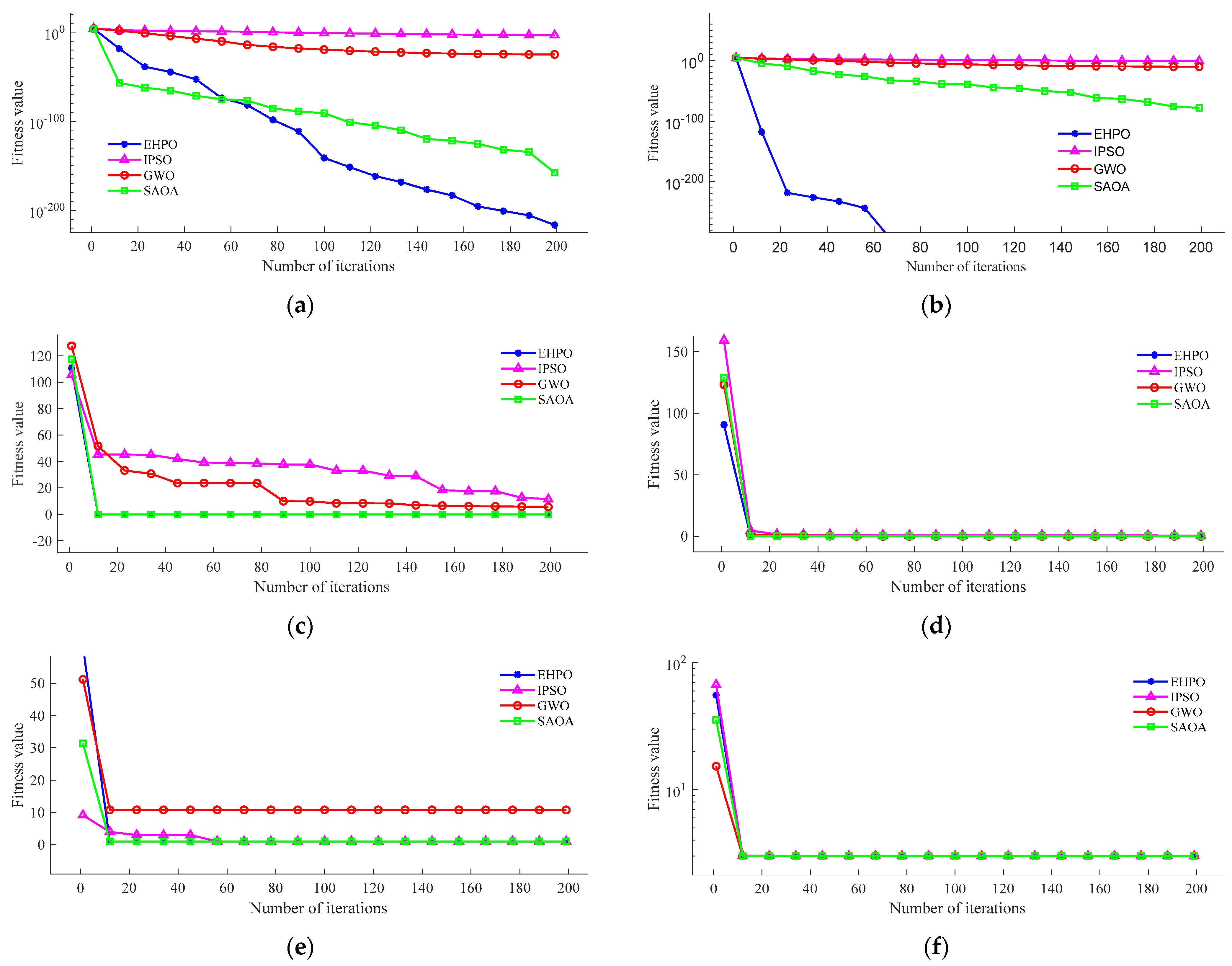
We chose the IPSO [15], GWO [34], and improved arithmetic optimization algorithm (SAOA) [35] as benchmark algorithms. These algorithms demonstrate an excellent performance. They each represent a specific class of optimisation strategies and ideas, and so the selection of these algorithms provides a comprehensive benchmark against which to assess the performance of EHPO. All algorithms have the same number of iterations and population size, with the number of iterations set to 200 and the population size set to 50. Other parameters were set according to the recommendations in the literature. The final results are shown in Figure 8.

The results in Figure 8 provide insights into the performance of the EHPO algorithm on different types of test functions:

• Unimodal test functions 1 and 2: In these two tests, EHPO shows good performance, successfully finding the minimum value among the four algorithms, and converging the fastest. This indicates that EHPO has a strong optimization ability and fast convergence speed on unimodal problems, and can effectively locate the global optimal solution.
• Multimodal test functions 3 and 4: The design of multimodal test functions contains multiple local optimal solutions, which poses a challenge to the global search ability of the algorithm. In test function 3, both EHPO and SAOA can find the minimum value, indicating that these two algorithms perform well in escaping local optima. In test function 4, all four algorithms find the minimum value, but EHPO has the fastest convergence speed in this test, showing its efficient performance on multimodal problems. In contrast, SAOA shows the best convergence speed in test function 3, which means that SAOA has advantages in some multimodal problems.
• Hybrid test functions 5 and 6: Hybrid test functions further increase the complexity of the problem. In test function 5, except for GWO, all other algorithms find the optimal value, and EHPO and SAOA have the fastest convergence speed, indicating that they maintain efficient search capabilities when dealing with complex search spaces. For test function 6, the performance differences between the four algorithms are not significant.

In summary, EHPO shows an excellent performance on both unimodal and multimodal test functions, especially in terms of convergence speed. At the same time, it also shows a comparable or superior performance regarding hybrid test functions. These results indicate that EHPO is a powerful and flexible optimization tool that performs well in different types of optimization problems.

6. Industrial Implications

The findings of this research have had a favourable impact on the industrial sector, which can be observed on multiple levels. Firstly, by enhancing the accuracy and universality of the fault warning system, firms can achieve more stable and reliable production processes. This translates into the better execution of production plans, more efficient utilisation of resources, and higher levels of product quality control, thereby boosting the firm’s production efficiency and competitiveness. Secondly, by reducing maintenance costs and production disruptions, firms can better manage their operating costs and increase profitability. These savings can be reinvested in technological innovation, staff training, and other areas, further fostering the development and growth of the firm. Additionally, improving the safety and comfort of the working environment helps to increase employee job satisfaction and loyalty and reduce staff turnover, thereby stabilising the production team and ensuring the continuity of production. Furthermore, steering the industry in a more sustainable direction aids in reducing resource wastage and environmental pollution, thereby making a positive contribution to the sustainable development of society and the environment. In summary, the results of this research not only hold significant value for the firm itself but also have an important positive impact on society and the environment as a whole.

7. Conclusions and Future Work

This study is focused on predicting and responding to potential equipment failures within the realm of industrial equipment fault early warning. We developed a comprehensive approach that combines deep learning techniques with metaheuristic algorithms, enhancing the accuracy and practicality of the early warning system. The Bi-LSTM is central to this method, acting as a powerful RNN that processes and predicts complex patterns in time series data. Its design leverages the dependencies of time series data in both directions, allowing for the more precise detection of subtle operational changes. In model construction and optimisation, we addressed the challenge of selecting optimal hyperparameters by using the EHPO algorithm. EHPO’s iterative process improves search efficiency and strengthens the model’s robustness against complex data.

Our method was validated in actual industrial environments, and the analysis of case datasets indicates that our approach achieves good fault warning effects. Moreover, through comparison with other advanced algorithms, our method shows a clear advantage in terms of predictive accuracy and also achieves satisfactory results in terms of indicators such as RMSE and MAE. These research findings confirm the effectiveness of the method and its potential in the early detection and prevention of equipment failures, reduction in downtime, and improvements in production efficiency and economic benefits.

Whilst our research has made significant strides in the field of industrial equipment fault warning, we recognise that as industrial technology continues to evolve and the types of equipment and fault patterns diversify, handling complex and diverse data will pose a challenge [4,36]. Our model needs to have stronger adaptability and generalisation capabilities. At the same time, the hyperparameter optimisation process may require substantial computational resources and time. In the future, we will explore the use of more complex deep learning models and more advanced data processing methods to enhance the adaptability and robustness of the model. We will also consider using more efficient hyperparameter optimisation algorithms to improve the search efficiency and model performance. Furthermore, we will research how to extend our approach to various industrial scenarios and consider integrating advanced machine learning technologies, such as transfer learning and meta-learning, to develop a more powerful and flexible equipment fault early warning system [37,38,39,40].

References

- Ji, Z.; Gan, H.; Liu, B. A deep learning-based fault warning model for exhaust temperature prediction and fault warning of marine diesel engine. J. Mar. Sci. Eng. 2023, 11, 1509. [Google Scholar] [CrossRef]
- Jieyang, P.; Kimmig, A.; Dongkun, W.; Niu, Z.; Zhi, F.; Jiahai, W.; Liu, X.; Ovtcharova, J. A systematic review of data-driven approaches to fault diagnosis and early warning. J. Intell. Manuf. 2023, 34, 3277–3304. [Google Scholar] [CrossRef]
- Fan, L.; Li, J.; Pan, Y.; Wang, S.; Yan, C.; Yao, D. Research and application of smart grid early warning decision platform based on big data analysis. In Proceedings of the 2019 4th International Conference on Intelligent Green Building and Smart Grid (IGBSG), Hubei, China, 6–9 September 2019; IEEE: Piscataway, NJ, USA, 2019; pp. 645–648. [Google Scholar]
- Hu, M.; He, Y.; Lin, X.; Lu, Z.; Jiang, Z.; Ma, B. Digital twin model of gas turbine and its application in warning of performance fault. Chin. J. Aeronaut. 2023, 36, 449–470. [Google Scholar] [CrossRef]
- Böse, M.; Andrews, J.; Hartog, R.; Felizardo, C. Performance and next-generation development of the finite-fault rupture detector (FinDer) within the United States West Coast ShakeAlert warning system. Bull. Seismol. Soc. Am. 2023, 113, 648–663. [Google Scholar] [CrossRef]
- Qiao, L.; Zhang, Y.; Wang, Q. Fault detection in wind turbine generators using a meta-learning-based convolutional neural network. Mech. Syst. Signal Process. 2023, 200, 110528. [Google Scholar] [CrossRef]
- Adam, S.P.; Alexandropoulos SA, N.; Pardalos, P.M.; Vrahatis, M.N. No free lunch theorem: A review. In Approximation and Optimization: Algorithms, Complexity and Applications; Springer: Berlin/Heidelberg, Germany, 2019; pp. 57–82. [Google Scholar]
- Lyu, N.; Jin, Y.; Miao, S.; Xiong, R.; Xu, H.; Gao, J.; Liu, H.; Li, Y.; Han, X. Fault warning and location in battery energy storage systems via venting acoustic signal. IEEE J. Emerg. Sel. Top. Power Electron. 2021, 11, 100–108. [Google Scholar] [CrossRef]
- Peng, H.; Zhang, H.; Fan, Y.; Shangguan, L.; Yang, Y. A review of research on wind turbine bearings’ failure analysis and fault diagnosis. Lubricants 2022, 11, 14. [Google Scholar] [CrossRef]
- Yang, Y.; Liu, A.; Xin, H.; Wang, J. Fault early warning of wind turbine gearbox based on multi-input support vector regression and improved ant lion optimization. Wind. Energy 2021, 24, 812–832. [Google Scholar] [CrossRef]
- Chen, S.; Ma, Y.; Ma, L. Fault early warning of pitch system of wind turbine based on GA-BP neural network model. E3S Web Conf. 2020, 194, 03005. [Google Scholar] [CrossRef]
- Lu, G.; Wen, X.; He, G.; Yi, X.; Yan, P. Early fault warning and identification in condition monitoring of bearing via wavelet packet decomposition coupled with graph. IEEE/ASME Trans. Mechatron. 2021, 27, 3155–3164. [Google Scholar] [CrossRef]
- Li, J.; Liu, J.; Chen, Y. A fault warning for inter-turn short circuit of excitation winding of synchronous generator based on GRU-CNN. Glob. Energy Interconnect. 2022, 5, 236–248. [Google Scholar] [CrossRef]
- Jing, N.; Li, H.; Zhao, Z. A microservice fault identification method based on LightGBM. In Proceedings of the 2022 IEEE 8th International Conference on Cloud Computing and Intelligent Systems (CCIS), Chengdu, China, 26–28 November 2022; IEEE: Piscataway, NJ, USA, 2022; pp. 709–713. [Google Scholar]
- Sun, Y.; Wang, L.; Lei, Q.; Cao, Q. Research on Vibration Prediction of Hydroelectric Turbine Units Based on CEEMDAN-IPSO-LSTM. People’s Yellow River 2023, 45, 156–162. [Google Scholar]
- Zhao, H.; Liu, H.; Hu, W.; Yan, X. Anomaly detection and fault analysis of wind turbine components based on deep learning network. Renew. Energy 2018, 127, 825–834. [Google Scholar] [CrossRef]
- Chen, H.; Li, S.; Li, M. Multi-Channel High-Dimensional Data Analysis with PARAFAC-GA-BP for Nonstationary Mechanical Fault Diagnosis. Int. J. Turbomach. Propuls. Power 2022, 7, 19. [Google Scholar] [CrossRef]
- Wang, H.; Chen, J.; Zhu, X.; Song, L.; Dong, F. Early warning of reciprocating compressor valve fault based on deep learning network and multi-source information fusion. Trans. Inst. Meas. Control 2023, 45, 777–789. [Google Scholar] [CrossRef]
- Cai, J.; Cai, Y.; Cai, H.; Shi, S.; Lin, Y.; Xie, M. Feeder fault warning of distribution network based on XGBoost. J. Phys. Conf. Ser. 2020, 1639, 012037. [Google Scholar] [CrossRef]
- Liu, J.; Cao, J.; Zhao, X. Fault Early Warning for Wind Turbine Gearbox Based on OOB-GWO-SVR. J. Electron. Meas. Instrum. 2022, 36, 97–105. [Google Scholar] [CrossRef]
- Fu, Y.; Liu, Y.; Yang, Y. Multi-sensor GA-BP algorithm based gearbox fault diagnosis. Appl. Sci. 2022, 12, 3106. [Google Scholar] [CrossRef]
- Liu, L.; Wan, X.; Gao, Z.; Zhang, X. An improved MPGA-ACO-BP algorithm and comprehensive evaluation system for intelligence workshop multi-modal data fusion. Adv. Eng. Inform. 2023, 56, 101980. [Google Scholar] [CrossRef]
- Hu, Y.; Wei, R.; Yang, Y.; Li, X.; Huang, Z.; Liu, Y.; He, C.; Lu, H. Performance degradation prediction using LSTM with optimized parameters. Sensors 2022, 22, 2407. [Google Scholar] [CrossRef]
- Le, T.; Vo, M.T.; Vo, B.; Hwang, E.; Rho, S.; Baik, S.W. Improving electric energy consumption prediction using CNN and Bi-LSTM. Appl. Sci. 2019, 9, 4237. [Google Scholar] [CrossRef]
- Naruei, I.; Keynia, F.; Sabbagh Molahosseini, A. Hunter–prey optimization: Algorithm and applications. Soft Comput. 2022, 26, 1279–1314. [Google Scholar] [CrossRef]
- Zu, L.; Wang, Z.; Liu, C.; Ge, S.S. Research on UAV path planning method based on improved HPO algorithm in multi-task environment. IEEE Sens. J. 2023, 23, 19881–19893. [Google Scholar] [CrossRef]
- Ye, Z.; Zhao, H.; Zhang, K.; Zhu, Y.; Xiao, Y.; Wang, Z. Improved DeepWalk Algorithm Based on Preference Random Walk. In Proceedings of the CCF International Conference on Natural Language Processing and Chinese Computing, Dunhuang, China, 9–14 October 2019; Springer International Publishing: Cham, Switzerland, 2019; pp. 265–276. [Google Scholar]
- Ouyang, C.; Qiu, Y.; Zhu, D. Adaptive spiral flying sparrow search algorithm. Sci. Program. 2021, 2021, 6505253. [Google Scholar] [CrossRef]
- Zhang, S.; Zheng, D.; Hu, X.; Yang, M. Bidirectional long short-term memory networks for relation classification. In Proceedings of the 29th Pacific Asia Conference on Language, Information and Computation, Shanghai, China, 30 October–1 November 2015; pp. 73–78. [Google Scholar]
- Fu, M.; Liu, Q. An Improved Hunter-prey Optimization Algorithm and Its Application. In Proceedings of the 2022 IEEE International Conference on Networking, Sensing and Control (ICNSC), Shanghai, China, 15–18 December 2022; IEEE: Piscataway, NJ, USA, 2022; pp. 1–7. [Google Scholar]
- Suebsombut, P.; Sekhari, A.; Sureephong, P.; Belhi, A.; Bouras, A. Field data forecasting using LSTM and Bi-LSTM approaches. Appl. Sci. 2021, 11, 11820. [Google Scholar] [CrossRef]
- Luan, L.; Tan, L.; Niu, B. A novel hybrid global optimization algorithm based on particle swarm optimization and differential evolution algorithms. Inf. Control. 2007, 36, 708–714. [Google Scholar]
- Tian, G.; Liu, J.; Zhang, X.; Pham, D.T.; Guo, X.; Du, Y.; Zhao, C.; Li, H. Multi-objective disassembly line design and optimisation considering energy efficiency and human factors. J. Eng. Des. 2024, 1–29. [Google Scholar] [CrossRef]
- Mirjalili, S.; Mirjalili, S.M.; Lewis, A. Grey wolf optimizer. Adv. Eng. Softw. 2014, 69, 46–61. [Google Scholar] [CrossRef]
- Li, S.; Jin, N.; Dogani, A.; Yang, Y.; Zhang, M.; Gu, X. Enhancing LightGBM for Industrial Fault Warning: An Innovative Hybrid Algorithm. Processes 2024, 12, 221. [Google Scholar] [CrossRef]
- Huang, C.; Qu, S.; Ke, Z.; Zheng, W. Dual fault warning method for coal mill based on Autoformer WaveBound. Reliab. Eng. Syst. Saf. 2024, 245, 110030. [Google Scholar] [CrossRef]
- Shen, S.; Sadoughi, M.; Li, M.; Wang, Z.; Hu, C. Deep convolutional neural networks with ensemble learning and transfer learning for capacity estimation of lithium-ion batteries. Appl. Energy 2020, 260, 114296. [Google Scholar] [CrossRef]
- Liu, X.; Liu, Z.; Wang, G.; Cai, Z.; Zhang, H. Ensemble transfer learning algorithm. IEEE Access 2017, 6, 2389–2396. [Google Scholar] [CrossRef]
- Xue, D.; Zhou, X.; Li, C.; Yao, Y.; Rahaman, M.; Zhang, J.; Chen, H.; Zhang, J.; Qi, S.; Sun, H. An application of transfer learning and ensemble learning techniques for cervical histopathology image classification. IEEE Access 2020, 8, 104603–104618. [Google Scholar] [CrossRef]
- Tian, G.; Zhang, C.; Zhang, X.; Feng, Y.; Yuan, G.; Peng, T.; Pham, D.T. Multi-objective evolutionary algorithm with machine learning and local search for an energy-efficient disassembly line balancing problem in remanufacturing. J. Manuf. Sci. Eng. 2023, 145, 051002. [Google Scholar] [CrossRef]
Figure 1.
Method execution framework.
Figure 2.
Data collection interface.
Figure 3.
A comparison of actual and predicted values.
Figure 4.
Residual trends and fault threshold determination.
Figure 5.
Model fault warning result.
Figure 6.
Comparison of standard deviations for three metrics across four algorithms.
Figure 7.
Comparison of RPD across six algorithms.
Figure 8.
Benchmark function testing results: Function 1 (a), Function 2 (b), Function 3 (c), Function 4 (d), Function 5 (e) and Function 6 (f).