TPTM-HANN-GA: A Novel Hyperparameter Optimization Framework Integrating the Taguchi Method, an Artificial Neural Network, and a Genetic Algorithm for the Precise Prediction of Cardiovascular Disease Risk

Abstract

The timely and precise prediction of cardiovascular disease (CVD) risk is essential for effective prevention and intervention. This study proposes a novel framework that integrates the two-phase Taguchi method (TPTM), the hyperparameter artificial neural network (HANN), and a genetic algorithm (GA) called TPTM-HANN-GA. This framework efficiently optimizes hyperparameters for an artificial neural network (ANN) model during the training stage, significantly enhancing prediction accuracy for cardiovascular disease (CVD) risk. The proposed TPTM-HANN-GA framework requires far fewer experiments than a traditional grid search, making it highly suitable for application in resource-constrained, low-power computers, and edge artificial intelligence (edge AI) devices. Furthermore, the proposed TPTM-HANN-GA framework successfully identified the optimal configurations for the ANN model’s hyperparameters, resulting in a hidden layer of 4 nodes, a tanh activation function, an SGD optimizer, a learning rate of 0.23425849, a momentum rate of 0.75462782, and seven hidden nodes. This optimized ANN model achieves 74.25% accuracy in predicting the risk of cardiovascular disease, which exceeds the existing state-of-the-art GA-ANN and TSTO-ANN models. The proposed TPTM-HANN-GA framework enables personalized CVD prediction to be efficiently conducted on low-power computers and edge-AI devices, achieving the goal of point-of-care testing (POCT) and empowering individuals to manage their heart health effectively.

1. Introduction

Cardiovascular disease (CVD) poses a significant public health challenge, with profound implications for both individuals and communities, resulting in substantial mortality rates and societal impact. A range of cardiovascular disorders, including coronary artery disease, myocardial infarction (heart attacks), strokes, arrhythmias, heart failure, and atherosclerosis, present a substantial menace to human health [1]. These conditions disrupt the normal function of the heart and blood vessels, impairing blood and oxygen delivery and causing significant damage to various bodily systems [2]. Consider the impact of narrowed arteries depriving the heart of oxygen and nutrients in coronary artery disease, the irregular electrical signals leading to arrhythmias, or the weakened pumping ability of the heart in heart failure, leaving individuals struggling to breathe. A stroke, characterized by a sudden interruption of blood flow to the brain, can strip individuals of language, movement, and essential functions. Meanwhile, atherosclerosis, operating silently, accumulates plaque in arteries, constricts blood flow, and increases the risk of events [3].

Cardiovascular diseases (CVDs) do not arise from isolated factors but rather from a complex network of interconnected risk elements. High blood pressure, cholesterol, and diabetes often collaborate, intensifying each other’s adverse impacts [4]. We require a multi-faceted strategy that addresses all contributing factors collectively rather than addressing each risk element in isolation. Engaging in unhealthy behaviors, such as poor diet, smoking, and excessive alcohol consumption, exacerbates the risk of CVD [5,6,7]. Individual choices and behaviors play a pivotal role in determining cardiovascular health outcomes. The solution rests in adopting healthier behaviors: consuming balanced diets, engaging in regular physical activity, quitting smoking, and moderating alcohol intake. However, prevention alone is insufficient. Detecting cardiovascular diseases (CVDs) at an early stage allows for timely intervention to prevent their severe impact.

Early detection poses a significant challenge in combating cardiovascular diseases (CVDs) [8,9,10]. Unlike diseases with clear and recognizable symptoms, CVDs often present as subtle signs, such as fatigue, chest discomfort, or general stress—easily dismissed in the hustle of daily life. These ambiguous indicators often fail to prompt proactive medical intervention, leading to disease. Compounding this challenge, certain CVDs progress gradually. Atherosclerosis, for example, deposits plaque in arteries, obstructing blood flow and revealing its destructive consequences much later on. Effective screening tools do exist but often require specialized equipment and trained professionals, resources that are not readily available in regions with limited resources. This reality means that essential examinations, such as electrocardiograms, blood tests, and cardiac ultrasounds, become inaccessible, further reducing the likelihood of early detection.

The accurate prediction of cardiovascular diseases (CVDs) can help healthcare professionals identify high-risk individuals before the onset of clinical symptoms. By analyzing a comprehensive set of CVD risk factors, predictive models can be constructed to estimate an individual’s susceptibility to this often silent condition [11,12,13,14]. This method empowers clinicians to prioritize patient monitoring and implement preventative measures. Tailored medical interventions and personalized health management recommendations can then be established for each patient. Early detection through such predictive models provides a valuable opportunity for treatment, facilitating interventions such as targeted lifestyle modifications (e.g., diet and exercise programs) and stress management strategies [15]. By adopting these proactive measures, individuals identified as high-risk can significantly reduce their CVD risk and take greater control of their overall well-being.

Additionally, pharmacological interventions become viable options, further lowering the risk of cardiovascular events [16]. Ultimately, early prediction not only minimizes the incidence and severity of CVD but also empowers individuals to become active participants in their cardiovascular health. The effect of CVD prediction fosters public health awareness, prompting individuals to take ownership of their heart health. Understanding their susceptibility can prompt people to make positive changes, such as incorporating regular exercise, choosing healthier diets, and scheduling preventive check-ups with their doctors. This approach can significantly reduce their risk of developing health problems. This shift in behavior translates to a healthier population, placing less strain on healthcare systems. Predictive models empower healthcare professionals to become efficient stewards of limited resources. By anticipating demand and developing targeted prevention and treatment plans, we can optimize resource allocation, reduce hospitalization times, and minimize healthcare costs [17]. The early identification of high-risk individuals coupled with effective interventions alleviates the pressure on healthcare systems, creating a virtuous cycle of improved health outcomes and reduced long-term financial burdens.

Despite the appeal of early CVD prediction, the potential for erroneous outcomes cannot be overlooked. In the context of early CVD prediction, a misclassification of patients as high-risk can trigger a sequence of unwarranted interventions, resource misallocation, and psychological distress [18]. Considering the potential for undergoing extraneous medical procedures, the associated financial strain, and the consequent psychological burden, a cautious approach to early CVD prediction is warranted [19]. The converse scenario presents an equally significant challenge: the missed identification of genuinely high-risk individuals. This can lead to a critical delay in implementing essential interventions, potentially allowing for the disease to progress unabated. Furthermore, inaccurate predictions breed skepticism. This public distrust can hamper efforts to promote preventative measures and ultimately weaken the entire system [20]. Therefore, the pursuit of highly accurate CVD prediction is not just a scientific endeavor but an ethical imperative. We must strive to minimize false positives and negatives, ensuring the benefits outweigh the risks and upholding public trust in this invaluable tool.

Scholars such as Arroyo and Delima (2022) [21] have harnessed genetic algorithms to fine-tune artificial intelligence, boosting prediction accuracy by 5.08%. Kim (2021) [22] demonstrated the potential of smartwatch-derived data for CVD prevalence prediction, achieving promising results with a machine-learning approach utilizing support vector machines (SVMs). Khan et al. (2023) [23] investigated the efficacy of machine learning algorithms, specifically random forest, for CVD prediction. Their findings demonstrated promising performance in terms of both accuracy and sensitivity. Building on previous work, Moon et al. (2023) [24] achieved a breakthrough in cardiovascular disease (CVD) susceptibility prediction. Their approach, which combined advanced AI techniques such as the literature embedding with machine learning, not only delivered 96% accuracy but also shed light on the underlying genes and factors contributing to individual risk.

Cardiovascular disease (CVD) prediction has made significant strides in recent years, but achieving high accuracy with limited resources remains a challenge. This study tackles the critical barrier of computational costs in accurate cardiovascular disease (CVD) prediction. The proposed method empowers individuals by significantly reducing computing needs while maintaining high accuracy, thereby achieving the goal of real-time, individualized CVD risk stratification that is readily accessible to users, enabling the optimization of preventative interventions and transforming health surveillance. Moreover, the proposed method, enabled by a resource-efficient artificial neural network model, allows for precise individual risk assessment, facilitating timely interventions that improve quality of life and overall cardiovascular health. Whether at the doctor’s office or even at home, this further achieves the goal of accurate CVD prediction at the point of care.

2. Materials and Methods

2.1. TPTM-HANN-GA Framework

Enhancing the performance of CVD risk prediction algorithms is paramount. Traditionally, researchers rely on subjective judgment when choosing hyperparameter levels, often leading to limited improvements and inefficient resource allocation. Hence, to fully realize the capabilities of CVD prediction models, this study proposed an optimization framework that breaks free from the limitations of trial and error. By combining two powerful techniques, the two-phase Taguchi method (TPTM) and the hyperparameter artificial neural network (HANN), this framework aimed to systematically and efficiently identify the optimal hyperparameter configurations for CVD prediction models.

In lieu of an exhaustive grid search, TPTM prioritizes the identification of salient relationships between hyperparameters and model accuracy. This is achieved by strategically evaluating multiple hyperparameter levels simultaneously, minimizing the required number of experiments. This phase shines a light on how each hyperparameter influences accuracy, revealing valuable insights, such as the potential benefit of a higher momentum rate in artificial neural networks (ANNs). Leveraging the insights gleaned from TPTM, the HANN algorithm assumes responsibility for the optimization process. This specialized neural network acts to fine-tune the hyperparameters based on the discovered trends. Its learning capabilities allow it to pinpoint the optimal configuration for maximizing prediction accuracy. To further enhance the optimization process, the framework incorporates the genetic algorithm (GA). This evolutionary approach explores the hyperparameter space, leveraging the knowledge gained from the previous phase to identify even more promising configurations. The genetic algorithm (GA) leverages a bio-inspired approach, emulating natural selection to refine the hyperparameter search process. This iterative process converges towards superior solutions, as detailed in

Table 1. Algorithm table for related methods.

Algorithm	Description and Explanation
Taguchi Method	Define Problem: determine the system or process to be optimized and identify the performance characteristics to evaluate. Design Experiment: select factors and levels and construct a Taguchi orthogonal array for experimental design. Conduct Experiment: execute experiments based on the design plan and collect data on performance characteristics. Analyze Experiment Results: evaluate experiment results using methods such as signal-to-noise ratio and analysis of variance (ANOVA). Optimize Design: adjust factor levels based on analysis results to optimize the system or process design. Validate Design: validate the optimized design to ensure the system or process meets expected performance.
Artificial neural network	Initialization: initialize the network structure and parameters. Forward Propagation: compute the outputs of each layer based on input data. Calculate Loss: determine the difference between predicted and actual outputs. Backward Propagation: update the network’s parameters based on the loss. Training: repeat steps 2–4 using training data to optimize the network. Prediction: use the trained network to predict outputs for new data.
Genetic algorithm	Initialize: initialize a population by randomly generating initial individuals. Evaluate: calculate the fitness of each individual to assess the quality of their solutions. Selection: choose individuals with higher fitness as parents for reproduction using roulette wheel selection. Crossover: perform a two-point crossover between selected parents to produce new offspring. Mutation: mutation is applied to introduce randomness to the newly generated offspring. Update: replace selected individuals in the population with the newly generated offspring to form the next generation. Termination: check if termination criteria are met (e.g., reaching maximum iterations).

.

This collaborative framework, harnessing the strengths of TPTM, HANN, and GA, promises to revolutionize the optimization of CVD prediction models. This work transcends heuristic optimization approaches, leveraging a data-driven methodology to achieve enhanced accuracy and reliability in CVD prediction models. Consequently, this paves the way for improved clinical decision-making and potentially superior patient outcomes.

The analytical process in this study can be delineated into six distinct steps, as illustrated in Figure 1.

(1)

Problem Definition: The first step of this investigation delved into the heart of the data itself. We began by identifying the source of the dataset and exploring its origin and any inherent biases or limitations.

(2)

Unveiling Hyperparameter Trends through Initial-Phase Taguchi Method: The initial exploration of hyperparameter space utilized the Taguchi L₁₈(2¹ × 3⁷) design. This powerful tool let us efficiently explore diverse combinations for our artificial neural network (ANN) model used in cardiovascular disease (CVD) prediction. We employed a combination of experimental and analytical techniques, including orthogonal arrays, parameter response tables, graphs, and analysis of variance (ANOVA), to achieve two key goals:

(i)

Identify Improved Configurations: By analyzing accuracy data from various configurations, we aimed to pinpoint settings that enhance CVD prediction accuracy compared to the initial model.

(ii)

Discern Preferred Trends: Beyond specific configurations, we sought to uncover broader trends within each hyperparameter. This involved identifying whether increasing or decreasing a hyperparameter’s value generally led to better prediction results.

By these trends, we gained valuable insights into the behavior of our ANN model and could make informed decisions for further optimization in the next step.

(3)

Refinement with the Second-phase Taguchi Method: Building upon the initial trends identified, we launched a second-phase Taguchi method L₉(3⁴) to delve deeper into the promising hyperparameter space. This focused exploration aimed to recollect an enriched dataset that promisingly harbored the best hyperparameter configurations. By strategically confining the hyperparameter range based on the insights from the previous step, we increased the likelihood of capturing the optimal solution within this refined search space. This iterative approach, characteristic of the Taguchi method, allowed us to efficiently hone in on the most favorable parameter settings for our model. To build a hyperparameter artificial neural network (HANN) model with a diverse dataset, this study used the Monte Carlo method to enhance the accuracy. This probabilistic model introduces uncertainty, resulting in varied outcomes during the simulation and creating a more diverse dataset. A normal distribution probabilistic model was applied for the Monte Carlo data augmentation in this study.

(4)

Crafting the Hyperparameter Artificial Neural Network (HANN): The data harvested in Step 3 served as the foundation for building our hyperparameter neural network (HANN). This study proposed a streamlined HANN architecture with a single hidden layer. To pinpoint the optimal configuration for this network, we employed a grid search method. This strategy systematically evaluates numerous parameter combinations, guided by the goal of minimizing the root mean square error (RMSE) on the test set. Following the initial hyperparameter exploration via TPTM, the HANN algorithm leverages the identified trends to converge on the optimal architecture.

(5)

Using the Genetic Algorithm (GA) to Find the Best Hyperparameter Configurations for Accurate Cardiovascular Disease Risk Prediction: This study took optimization a step further by employing the genetic algorithm (GA) to determine the globally optimal configurations for the HANN model’s input variables. In contrast to grid search’s finite exploration, the genetic algorithm efficiently searches the hyperparameter space. This bio-inspired approach emulates natural selection, iteratively refining the population towards configurations that yield progressively enhanced robustness and accuracy in CVD risk prediction models. This broader search empowers the model to perform at its peak by considering a wider range of potential configurations.

(6)

Comparative Study: To validate the advancements achieved in this study, the highest model accuracy obtained through the TPTM-HANN-GA method was benchmarked against the accuracy of relevant models reported in the literature. This comparison provided a rigorous assessment of our proposed approach and its potential contributions to the field.

2.2. Literature Review

2.2.1. Artificial Neural Network (ANN)

Artificial neural networks can effectively learn and represent intricate patterns within data. These networks consist of interconnected nodes (neurons) arranged in layers. Each neuron receives signals from previous layers, processes them, and sends its own signal forward. This intricate web allows for ANNs to learn complex relationships [25,26,27,28]. However, two hyperparameters significantly impact their performance: learning rate and momentum. The learning rate controls how much the network adjusts its internal connections during training. If this rate is too high, the network becomes unstable, while a rate that is too low slows down learning or gets stuck in suboptimal solutions [29,30]. The momentum optimization technique accumulates historical gradient updates. This inertia smooths out fluctuations in the learning landscape, which is particularly beneficial for navigating complex problems with numerous local minima. By effectively utilizing this momentum term, the optimization process converges more efficiently.

Artificial neural networks have emerged for various modeling and prediction tasks across diverse fields. Katona T. et al. (2024) proposed an optimized deep learning model utilizing pre-trained CNNs and novel optimization strategies for multi-label classification of chest X-ray images, aiming to aid automated interpretation and support clinicians in their diagnoses [31]. Franchini, G. (2024) proposed a green approach to hyperparameter tuning in deep learning models, utilizing performance predictors to minimize computational costs and environmental impact, thereby accelerating the neural architecture search process and improving efficiency in tasks such as image denoising and classification [32]. Other studies have explored their potential in medical image segmentation tasks (Malhotra et al., 2022) [33], real-time classification of diversely packaged drugs (You et al., 2023) [34], toxicology research for predicting compound toxicity (Pantic et al., 2022) [35], classifying liver cancer from histopathology images (Lin et al., 2021) [36], lung cancer recognition (He et al., 2022) [37], and even predicting the outcome of diabetic foot ulcer treatments (Poradzka et al., 2023) [38]. Furthermore, research such as Krasteva et al. (2023) demonstrates their optimization capabilities for specific tasks such as arrhythmia classification [39]. These diverse applications showcase the wide-ranging potential of ANNs in various prediction and modeling domains.

2.2.2. Taguchi Method

The Taguchi method, developed by Dr. Genichi Taguchi in the 1950s, revolutionized quality management. Initially popular in Japan, it gained global recognition in the 1980s, becoming a cornerstone of robust design [40]. Dr. Taguchi’s early work laid the foundation for this approach, leading to significant improvements in product quality and cost [41,42]. The key innovation of the Taguchi method lies in its focus on “noise factors,” uncontrollable variables impacting product performance. Unlike traditional methods that solely address controllable factors, the Taguchi method seeks optimal parameter settings that minimize the impact of noise, leading to more robust and consistent products by utilizing orthogonal arrays. These special experimental designs allow researchers to gather comprehensive data with fewer experiments, improving the efficiency and result reliability [43]. In contemporary high-complexity manufacturing systems, achieving such optimization efficiency is paramount. Traditional methodologies often exhibit limitations in terms of protracted execution times and substantial resource requirements.

Traditional full factorial designs, where all possible combinations of factors are tested, can become time-consuming as the number of variables increases. This exponential growth in experiments poses a significant challenge for researchers seeking efficient solutions. Orthogonal arrays, introduced by Dr. Taguchi, are a powerful tool for streamlining experimentation. These designs allow researchers to study the effects of multiple factors with significantly fewer experiments, maintaining comprehensive and reliable data [43]. This efficiency is particularly valuable in today’s complex research environments, where time and resources are often limited. Furthermore, orthogonal arrays ensure experimental reproducibility. By ensuring specific properties in the experimental setup, these designs guarantee that experiments can be easily replicated and their results verified, boosting the overall reliability and validity of the findings.

Dr. Taguchi’s contribution involved applying the signal-to-noise ratio (SN), a well-established concept in telecommunications typically quantified in decibels (dB), to the domain of quality control. This innovative approach significantly reshaped quality management practices. This powerful metric exposed factors significantly affecting product quality during production [40]. A high SN ratio signified a robust process and exceptional quality, while a low one served as a red flag. Tailored to specific quality objectives, three distinct SN ratio types were employed:

(1) Nominal-the-better (NTB): Preferring values closest to a target (m).

$${\mathrm{S}\mathrm{N}}_{\mathrm{N}\mathrm{T}\mathrm{B}}=-10\mathit{log}\left[\frac{{\sum }_{i=1}^n(y_i-m{)}^2}{n}\right]=-10\mathit{log}\left[{{\left(\overline{y}-m\right)}^2+S}^2\right].$$

(1)

(2) Smaller-the-better (STB): Aiming for the smallest possible values.

$${\mathrm{S}\mathrm{N}}_{\mathrm{S}\mathrm{T}\mathrm{B}}=-10\mathit{log}\frac{{\sum }_{i=1}^n{y}_i^2}{n}=-10\mathit{log}({\overline{y}}^2+S^2).$$

(2)

(3) Larger-the-better (LTB): Seeking the largest possible values.

$${\mathrm{S}\mathrm{N}}_{\mathrm{L}\mathrm{T}\mathrm{B}}=-10\mathit{log}\frac{{\sum }_{i=1}^n\frac{1}{y_i^2}}{n}.$$

(3)

Formulas (1)–(3) used specific calculations to assess quality based on average values ($\overline{y}$), target values (m), variances (S²), individual values (y_i), and the number of treatments (n).

The Taguchi method’s versatility is gaining recognition as a powerful tool for optimizing diverse engineering challenges. In biosensing, Kaziz et al. (2023) [44] employed its L₈(2⁵) approach to significantly accelerate detection times under alternating current electrothermal forces. For medical imaging, Tseng et al. (2022) [45] successfully optimized brain tissue visualization using a custom PMMA slit gauge designed through the Taguchi method. Karimipourfard et al. (2024) [46] used the Taguchi method to improve a deep learning model for fast and accurate patient-specific internal dosimetry, achieving results comparable to the gold-standard Monte Carlo but with much faster calculation speed. Bayraktar et al. (2024) [47] applied the Taguchi method to optimize the production of bacterial nano-cellulose from whey waste, a sustainable approach yielding biocompatible and biodegradable nanomaterials with potential for biomedical applications. These diverse applications demonstrate the Taguchi method’s adaptability and potential to contribute to advancements across various engineering fields.

2.2.3. Genetic Algorithm

Introduced in 1975, the genetic algorithm (GA) has matured into a robust optimization paradigm. Leveraging principles inspired by natural selection, GAs excel at navigating intricate problem domains to identify optimal solutions. The GA iteratively refines a population of potential solutions, favoring those that perform well. This self-adapting approach excels in high-dimensional optimization, making it ideal for tasks such as hyperparameter tuning in machine learning and control variable refinement in engineering [48]. The GA’s evolutionary process involves three phases: chromosome reproduction, crossover (combining features), and mutation (introducing randomness). Within the solution space of an engineering challenge, the GA iteratively identifies the most versatile solution that meets all constraints, boasts the highest fitness function value, and represents the globally optimal solution [49].

The genetic algorithm (GA) is an effective tool for iterative optimization. It orchestrates a process that progressively refines candidate solutions towards achieving global optima within the search space. This iterative refinement commences with population initialization, where a collection of diverse candidate solutions is generated, constituting the initial population. This variety sets the stage for exploration across the solution space. Next, the evaluation stage assesses each solution’s performance through a fitness function, gauging its effectiveness within the problem context. The optimization process intensifies with the parent selection stage. During this stage, a selection mechanism prioritizes high-performing individuals within the population to become parents for the next generation. Parent selection mechanisms, such as roulette wheel selection or elite preservation, prioritize solutions with superior fitness scores, ensuring these desirable traits are carried forward. Subsequently, the crossover operation takes place. Here, genetic material from two selected parents is exchanged, resulting in offspring chromosomes that inherit a blend of valuable characteristics from both parents. This process of crossover is instrumental in maintaining population diversity and fostering the exploration of novel solution spaces. However, evolution needs variety, so mutation throws in controlled randomness, altering some offspring to prevent stagnation in local optima. Following the reproduction phase, a selection mechanism determines which individuals from the current generation (parents and offspring) will be incorporated into the subsequent generation’s population. This selection pressure ensures the population continuously evolves toward superior solutions. This cyclical refinement propels the search for better solutions. This iterative process continues until a predefined termination criterion is satisfied. This criterion can be based on achieving a satisfactory fitness score or exceeding a maximum number of generations. Each iteration facilitates the progressive refinement of the population towards superior solution states within the search space.

This study employed a structured chromosome format to represent control variable configurations. Each variable’s value was encoded as a binary gene, forming the building blocks of the chromosome. This efficient encoding facilitated manipulation and analysis within the experimental domain. To find optimal control settings, the GA leverages iterative crossover and mutation operations. These operations guide the current population toward the next generation, progressively approaching optimal settings or reaching a predefined limit [49]. The chosen two-point crossover creates novel chromosomes by exchanging genetic material between paired parents. Notably, crossover points remain consistent across genes within a chromosome. During mutation, a designated portion of each chromosome’s bits undergoes random changes (1 to 0 or vice versa). This systematic variation fosters convergence towards optimal solutions. The study’s objective function was adapted and transformed into a fitness function within the GA framework. Higher fitness values are directly associated with superior solution quality. Chromosomes with high fitness have a greater chance of generating offspring, promoting the propagation of promising genetic traits. The roulette wheel method further biases selection towards high-fitness chromosomes, accelerating the search for optimal solutions. This rewrite retained the key information while avoiding direct copying, achieving the desired originality and clarity.

The versatility of the genetic algorithm (GA) is demonstrably evident across a multitude of disciplines, as exemplified by the following contemporary applications. Neumann et al. (2023) [50] explored GA’s role in ETO challenges. They analyzed key characteristics, constraints, and objectives, delving into common encoding formats and genetic operators, with a particular focus on multi-objective approaches. Altarabichi et al. (2023) [51] tackled efficient feature selection in massive datasets by proposing a two-phase surrogate-assisted evolutionary approach powered by GA. This innovative method demonstrated effectiveness in sifting through large data volumes. Aziz et al. (2023) [52] introduced a novel approach combining GA and deep learning for highly accurate fraud detection in Ethereum smart contracts. Their method outperformed various popular techniques, showcasing the algorithm’s potential for enhancing financial security. Ghezelbash et al. (2023) [53] leveraged GA to improve mineral prospectivity mapping. They combined unsupervised clustering and supervised machine learning methods, demonstrating the algorithm’s adaptability to real-world geospatial applications.

3. Results

3.1. Dataset Description

This study employs the Kaggle Cardiovascular Disease dataset [54] to validate the proposed method for predicting the risk of cardiovascular disease. The dataset encompasses 70,000 medical records, each containing 12 variables (11 input features and 1 target variable). To optimize the training and testing of our ANN models, we implemented an 80% training and 20% testing split.

Table 2. Description of features in the Kaggle Cardiovascular Disease dataset [54].

Variable	Data Type
#1: Age	int (days)
#2: Height	int (cm)
#3: Weight	float (kg)
#4: Gender	categorical code
#5: Systolic blood pressure	int
#6: Diastolic blood pressure	int
#7: Cholesterol	1: normal, 2: above normal, 3: well above normal
#8: Glucose	1: normal, 2: above normal, 3: well above normal
#9: Smoking	binary
#10: Alcohol intake	binary
#11: Physical activity	binary
#12: Presence (or absence) of cardiovascular disease	binary

describes the comprehensive features of the Kaggle Cardiovascular Disease dataset.

(a)

An analysis of age distribution (measured in days) revealed distinct proportions across age groups. The youngest group (under 16,000 days) comprised 8159 individuals (11.66%). The 16,000–17,999-day range held 10,027 individuals (14.32%), followed by the 18,000–19,999-day group with 20,490 (29.27%). The 20,000–21,999-day range showed a similar number at 20,011 (28.59%), while the oldest group (22,000–24,000 days) included 11,313 individuals (16.16%).

(b)

An analysis of height distribution (in centimeters) showed a clear trend. The shortest group (under 150 cm) accounted for 1537 individuals (2.20%). The most common height range was 160–169 cm, with 33,463 individuals (47.80%). Heights between 150 and 159 cm and 170–179 cm were also well represented at 16,986 (24.27%) and 15,696 (22.42%), respectively. Taller individuals were less frequent, with 2213 (3.16%) between 180 and 189 cm and only 105 (0.15%) exceeding 190 cm.

(c)

An examination of weight distribution (in kilograms) uncovered a pattern. The lightest weight category (below 50 kg) included 987 individuals (1.41%). Weights between 50 and 69 kg were the most prevalent, with 27,864 individuals (39.81%) falling within this range (50–59 kg: 7174 at 10.25% and 60–69 kg: 20,690 at 29.56%). The 70–79 kg range was also significant at 19,476 (27.82%). Heavier weights were progressively less common, with 11,989 individuals (17.13%) between 80 and 89 kg, 5831 (8.33%) between 90 and 99 kg, and 3853 (5.50%) exceeding 100 kg.

(d)

An analysis of gender distribution revealed a skew towards females. There were 45,530 females, representing approximately 65.4% of the 70,000 patients. Males accounted for the remaining 34.96%, totaling 24,470 patients.

(e)

An analysis of systolic blood pressure readings showed a majority of individuals within a normal range. Specifically, 13,038 (18.63%) had readings below 120, while 37,561 (53.66%) fell between the healthy range of 120 and 139. Readings between 140 and 159, though considered elevated, were present in 14,436 individuals (20.62%). Only a small portion, 5.57% (3901) and 1.52% (1064) had readings between 160 and 179 and above 180, respectively, which are categorized as hypertension.

(f)

An analysis of diastolic blood pressure readings yielded a similar distribution to systolic blood pressure. A significant portion, 35,450 individuals (50.64%), exhibited readings within the normal range (80–89 mmHg). Similarly, a sizeable group, 14,116 (20.17%), had readings below 80 mmHg. While elevated diastolic pressure readings (90–99 mmHg) were present in 14,612 individuals (20.87%), readings categorized as hypertension (100 mmHg and above) were less common, affecting 5.91% (4139 individuals) between 100 and 109 mmHg and 2.40% (1683 individuals) above 110 mmHg.

(g)

An analysis of cholesterol levels revealed a positive trend, with the majority (74.84%, or 52,385 patients) having normal levels. However, a notable portion of the population, 13.64% (approximately 9549 patients), has above-normal cholesterol, and 11.52% (approximately 8066 patients) has well above-normal levels.

(h)

Similar to cholesterol, an analysis of glucose levels showed a positive trend. The majority of patients (84.97%, or 59,479 individuals) exhibited normal glucose levels. However, a combined percentage of 15.03% (7.41% above normal and 7.62% well above normal) had abnormal glucose levels.

(i)

The analysis of smoking habits reveals a positive public health trend. A very high proportion of patients (approximately 91.19%, or 63,831 individuals) are non-smokers. This is encouraging news, as smoking is a major risk factor for various health conditions. However, there is still a minority of patients (approximately 8.81%, or 6169 individuals) who smoke.

(j)

The prevalence of alcohol consumption is low in this patient population. A vast majority of patients (approximately 94.62%, or 66,236 individuals) reported no alcohol consumption. This is positive, as excessive alcohol consumption can contribute to various health problems. However, a small minority (approximately 5.38%, or 3764 individuals) do consume alcohol.

(k)

Encouragingly, a large majority of patients (approximately 80.37%, or 56,261 individuals) reported being physically active. This is a positive finding, as regular physical activity is associated with numerous health benefits, including a reduced risk of cardiovascular disease. However, a significant minority (approximately 19.63%, or 13,739 individuals) were inactive.

(l)

Nearly half (49.97%) of the patient population has cardiovascular disease (CVD). This highlights the importance of continued monitoring and preventative measures for this at-risk group.

Given the diverse nature of the input features, normalization is crucial to ensure consistent analysis and prevent biases: imbalanced scales can skew the model towards features with larger values. To address this, we adopted z-score normalization, a technique that standardizes features by transforming them onto a common scale with a mean of 0 and a standard deviation of 1. This not only improves accuracy by giving each feature equal weight during training but also enhances the robustness of our analytical evaluations across the entire feature set.

3.2. Unveiling Hyperparameter Trends through the Initial-Phase Taguchi Method

In Section 3.2 and Section 3.3, we refer to the part of the experimental results of the two-stage Taguchi optimization (TSTO) method (C. M. Lin and Y. S. Lin, 2023) [55]. This study follows the steps of TSTO and adds the Monte Carlo method to the second-stage Taguchi method of TSTO to expand the number of modeling data points. Therefore, this study refers to the modified method as the two-phase Taguchi method (TPTM) to distinguish it from the TSTO method.

To maximize the model’s predictive ability, we focused on six key hyperparameters influencing the artificial neural network (ANN): hidden layers (HL), activation function (AF), optimizer (OP), learning rate (LR), momentum rate (MR), and hidden nodes (HN). Their potential impact on performance is outlined in

Table 3. Hyperparameters’ levels for the L₁₈(2¹ × 3⁷) orthogonal array.

V1	V2	V3	V4	V5	V6
Level 1 = 4	Level 1 = logistic	Level 1 = lbfgs	Level 1 = 0.2	Level 1 = 0.7	Level 1 = 4
Level 2 = 8	Level 2 = tanh	Level 2 = sgd	Level 2 = 0.3	Level 2 = 0.8	Level 2 = 8
Level 3 = 12	Level 3 = relu	Level 3 = adam	Level 3 = 0.4	Level 3 = 0.9	Level 3 = 12

, where “level 1” represents the lower setting and “level 2” signifies the higher one. To identify optimal configurations and uncover broader trends, we leveraged the Taguchi method’s initial phase L₁₈(2¹ × 3⁷). This systematic approach evaluated various combinations of these hyperparameters (V₁ through V₆) within the L₁₈(2¹ × 3⁷) orthogonal array. By analyzing the resulting accuracy data, we aimed to pinpoint settings that lead to improved predictive performance compared to the initial model and discern general trends within each hyperparameter, guiding us toward more effective configurations in the next step.

The Taguchi design addresses the inherent randomness present in ANN training by incorporating noise as a controlled factor. This approach effectively improves the signal-to-noise ratio, mitigating random variations and ensuring consistent performance across training iterations. Employing a conventional grid search for six hyperparameters with three discrete levels, replicated three times, yields 2187 (3⁶ × 3) experiments. In contrast, the initial-phase Taguchi method in this study achieved the same goal with only 54 experiments, significantly reducing the computational burden. This efficiency allowed us to utilize an ultra-low-cost personal computer, detailed below, eliminating the need for high-end hardware or GPUs. This study used a low-power computer manufactured by Hewlett-Packard Company (Palo Alto, CA, USA). It was equipped with an i5-1135G7 @ 2.40 GHz processor, 8 GB RAM, 64-bit operating system. To perform our computations, we utilized Python 3.9.13 software, developed by the Python Software Foundation, (Wilmington, DE, USA).

By delving into the effects of each hyperparameter, we aimed to identify critical factors and uncover recurring patterns within their different settings. The impact effect of each hyperparameter is quantified by the maximum difference in the overall average SN ratio across its different levels. To comprehensively communicate these findings, we constructed both a table and a chart of hyperparameter responses, concisely summarizing the analysis of each hyperparameter’s influence.

Since our goal is to maximize the ANN model’s average accuracy (following the larger-the-better principle), we calculated the SN ratio for each experiment using Formula (3). The resulting SN ratios are presented in the last row of

Table 4. Results and application of the L₁₈(2¹ × 3⁷) orthogonal array.

Experiment		1	2	3	4	5	6	7	8	9	10	11	12	13	14	15	16	17	18
Hyperparameter	V1	4	4	4	8	8	8	12	12	12	4	4	4	8	8	8	12	12	12
	V2	logistic	tanh	relu	logistic	tanh	relu	logistic	tanh	relu	logistic	tanh	relu	logistic	tanh	relu	logistic	tanh	relu
	V3	lbfgs	sgd	adam	lbfgs	sgd	adam	sgd	adam	lbfgs	adam	lbfgs	sgd	sgd	adam	lbfgs	adam	lbfgs	sgd
	V4	0.2	0.3	0.4	0.3	0.4	0.2	0.2	0.3	0.4	0.4	0.2	0.3	0.4	0.2	0.3	0.3	0.4	0.2
	V5	0.7	0.8	0.9	0.8	0.9	0.7	0.9	0.7	0.8	0.8	0.9	0.7	0.7	0.8	0.9	0.9	0.7	0.8
	V6	4	8	12	12	4	8	8	12	4	8	12	4	12	4	8	4	8	12
Accuracy	N1	0.4951	0.7389	0.4951	0.4951	0.7404	0.4951	0.4951	0.4951	0.7341	0.4951	0.7361	0.7389	0.5049	0.4951	0.7416	0.4951	0.7441	0.7384
	N2	0.4951	0.7382	0.5049	0.4951	0.7405	0.4951	0.5049	0.4951	0.7414	0.4951	0.7386	0.7381	0.4951	0.5049	0.7412	0.4951	0.7418	0.724
	N3	0.4951	0.7262	0.4951	0.4951	0.7331	0.4951	0.5049	0.5136	0.4951	0.4951	0.7372	0.7404	0.4951	0.4951	0.7404	0.4951	0.7423	0.7431
Average Accuracy		0.4951	0.7345	0.4984	0.4951	0.738	0.4951	0.5016	0.5013	0.6569	0.4951	0.7373	0.7391	0.4984	0.4984	0.7411	0.4951	0.7427	0.7352
Standard Deviation		0.0000	0.0071	0.0056	0.0000	0.0043	0.0000	0.0056	0.0106	0.1401	0.0000	0.0013	0.0012	0.0056	0.0056	0.0007	0.0000	0.0012	0.01
Signal-to-Noise Ratio		−6.105	−2.682	−6.050	−6.105	−2.639	−6.105	−5.994	−6.002	−4.124	−6.105	−2.647	−2.626	−6.050	−6.050	−2.603	−6.105	−2.584	−2.674

. Next, we delve further into the hyperparameter effects by examining the table of hyperparameter response (

Table 5. Table of hyperparameter response for the average of SN Ratio in L₁₈(2¹ × 3⁷) orthogonal array.

Hyperparameter	V1	V2	V3	V4	V5	V6
Average of signal-to-noise ratio	Level 1 = −4.369	Level 1 = −6.078	Level 1 = −4.028	Level 1 = −4.929	Level 1 = −4.912	Level 1 = −4.608
	Level 2 = −4.925	Level 2 = −3.767	Level 2 = −3.777	Level 2 = −4.354	Level 2 = −4.623	Level 2 = −4.345
	Level 3 = −4.581	Level 3 = −4.030	Level 3 = −6.070	Level 3 = −4.592	Level 3 = −4.340	Level 3 = −4.921
Effect	0.556	2.311	2.293	0.575	0.572	0.576
Rank	6	1	2	4	5	3

The effect of each hyperparameter is quantified by the maximum difference in the overall average SN ratio across its different levels.

) and the chart of the hyperparameter response (Figure 2). These visualization tools help us understand how varying each hyperparameter level affects the model’s SN ratio. Finally, to statistically assess the significance of these effects, we conducted an ANOVA analysis (presented in

Table 6. Hyperparameter ANOVA table for the SN ratio in L₁₈(2¹ × 3⁷) array.

Hyperparameter	Degrees of Freedom	Sum of Squares	Mean of Squares	F-Value	p-Value
V1	2	0.946	0.473	0.35	0.718
V2	2	19.195	9.597	7.20	0.034
V3	2	18.972	9.486	7.12	0.034
V4	2	1.003	0.502	0.38	0.704
V5	2	0.983	0.491	0.37	0.709
V6	2	0.998	0.499	0.37	0.706
Error	5	6.665	1.333
Sum	17	48.761
				R2	R2 (adjust)
				86.33%	53.53%

ANOVA, analysis of variance.

). This statistical test provides valuable insights into which hyperparameters have the most substantial impact on the model’s performance.

The analysis in Table 5 reveals a hierarchy of hyperparameter influence on the ANN’s SN ratio, with V₂ (AF) and V₃ (OP) emerging as the most critical factors (p < 0.1 in Table 6). Figure 2 visually confirms this, showcasing “tanh” for V₂ (AF) and “sgd” for V₃ (OP) as optimal configurations alongside favorable settings for V₄ (LR), V₅ (MR), and V₆ (HN). Notably, the best configuration for V₁ (HL) lies at level 1 (4 hidden layers), denoted as V₁(1). The optimized model architecture consists of six variables: V₁(1), V₂(2), V₃(2), V₄(2), V₅(3), and V₆(2). This configuration translates to a four-hidden-layer network with eight hidden nodes per layer, resulting in the 11-8-8-8-8-1 architecture shown in Figure 3.

3.3. Refinement with the Second-Phase Taguchi Method

Analyzing Figure 2 revealed that four hidden layers (V₁) yielded the best SN ratio. Prioritizing accuracy, we fixed V₁ at four layers to avoid compromising the performance. Additionally, the ANOVA identified V₂ (AF) and V₃ (OP) as key categorical variables, which were set to tanh and sgd, respectively, for optimal results. Further insights from Figure 2 suggested that settings of 0.3, 0.9, and 8 for V₄ (LR), V₅ (MR), and V₆ (HN), respectively, led to improvements in both accuracy and SN ratio. Building upon these findings, the second-phase Taguchi method aimed to refine these configurations and promisingly discover even better configurations. We maintained the optimal setting V₁ (HL) = 4 and assigned the optimal values for categorical variables (V₂ = tanh, V₃ = sgd) identified earlier. For the remaining hyperparameters (V₄, V₅, V₆), we investigated a range of values around their previously identified optimal settings, looking for potential improvements.

Table 7. Hyperparameters’ levels in the L₉(3⁴) orthogonal array.

V4	V5	V6
Level 1 = 0.25	Level 1 = 0.85	Level 1 = 6
Level 2 = 0.3	Level 2 = 0.9	Level 2 = 8
Level 3 = 0.35	Level 3 = 0.95	Level 3 = 10

summarizes the hyperparameters and their exploration ranges for this step.

The Taguchi method’s efficiency shines through its use of the orthogonal array L₉(3⁴). As presented in

Table 8. Results and application of the L₉(3⁴) orthogonal array.

Experiment		1	2	3	4	5	6	7	8	9
Hyperparameter	V4	0.25	0.25	0.25	0.3	0.3	0.3	0.35	0.35	0.35
	V5	0.85	0.9	0.95	0.85	0.9	0.95	0.85	0.9	0.95
	V6	6	8	10	8	10	6	10	6	8
Accuracy	N1	0.739	0.7392	0.7348	0.7348	0.7399	0.7357	0.7418	0.7376	0.742
	N2	0.7379	0.7381	0.7414	0.7411	0.7341	0.736	0.7349	0.7301	0.7374
	N3	0.7417	0.7376	0.7398	0.7399	0.74	0.7395	0.7388	0.7374	0.7291
Average Accuracy		0.7395	0.7383	0.7387	0.7386	0.738	0.7371	0.7385	0.735	0.7361
Standard Deviation		0.002	0.0008	0.0035	0.0033	0.0034	0.0021	0.0035	0.0043	0.0065
Signal-to-Noise Ratio		−2.621	−2.635	−2.631	−2.632	−2.639	−2.650	−2.633	−2.675	−2.661

, each hyperparameter was assigned to a column, enabling efficient exploration with minimal experiments. This approach required only 27 experiments (9 runs with three repeats), compared to the 81 experiments needed for a grid search with three levels and three repeats per hyperparameter. Through this refined exploration, we gathered valuable data with potential optimal solutions for our model hyperparameters.

In order to construct a hyperparameter ANN model using a large and diverse dataset, this study employed the Monte Carlo method [56] to enhance the accuracy of data from Table 8. The Monte Carlo method is a probabilistic model that incorporates uncertainty or stochastic elements in its predictions. Therefore, when using a probabilistic model to simulate outcomes, different results will be obtained each time, allowing for the generation of a more diverse dataset. In this study, a normal distribution probabilistic model was utilized for the Monte Carlo method data augmentation, and the results of the data augmentation are presented in

Table 9. Results of Monte Carlo method.

Experiment		1	2	3	4	5	6	7	8	9
Hyperparameter	V4	0.25	0.25	0.25	0.3	0.3	0.3	0.35	0.35	0.35
	V5	0.85	0.9	0.95	0.85	0.9	0.95	0.85	0.9	0.95
	V6	6	8	10	8	10	6	10	6	8
Accuracy	N1	0.739	0.7392	0.7348	0.7348	0.7399	0.7357	0.7418	0.7376	0.742
	N2	0.7379	0.7381	0.7414	0.7411	0.7341	0.736	0.7349	0.7301	0.7374
	N3	0.7417	0.7376	0.7398	0.7399	0.74	0.7395	0.7388	0.7374	0.7291
Average Accuracy		0.7395	0.7383	0.7387	0.7386	0.738	0.7371	0.7385	0.735	0.7361
Standard Deviation		0.002	0.0008	0.0035	0.0033	0.0034	0.0021	0.0035	0.0043	0.0065
P1		0.7389	0.7387	0.7395	0.7357	0.7338	0.7376	0.7365	0.7402	0.7347
P2		0.7397	0.7378	0.7449	0.7343	0.7363	0.7363	0.7443	0.7396	0.7251
P3		0.74	0.7367	0.7394	0.7418	0.7416	0.737	0.7383	0.7314	0.7474
P4		0.7403	0.7384	0.7447	0.7383	0.7379	0.7381	0.7407	0.7387	0.7378
P5		0.7422	0.7361	0.7376	0.7354	0.7425	0.7356	0.7338	0.7422	0.7344
P6		0.7389	0.7383	0.7399	0.7439	0.7329	0.737	0.74	0.7345	0.7346
P7		0.7423	0.7381	0.7397	0.7398	0.7415	0.7386	0.7385	0.7318	0.7287
P8		0.7397	0.738	0.7428	0.7375	0.7372	0.7345	0.7397	0.7374	0.733
P9		0.7404	0.738	0.7366	0.7412	0.7394	0.7361	0.7354	0.735	0.7287
P10		0.7384	0.7366	0.7388	0.7316	0.7376	0.7361	0.7323	0.7339	0.7446

, rows P₁ to P₁₀.

3.4. Crafting the Hyperparameter Artificial Neural Network (HANN)

The HANN model in Figure 4 uses learning rate (V₄), momentum rate (V₅), and hidden nodes (V₆) as input variables to predict cardiovascular disease accuracy. Its output variable is the accuracy value from Table 9. The dataset for the HANN model is sourced from Table 9. This study proposes a single-hidden-layer HANN model. The data are randomly split into 80% for training and 20% for testing. The model uses the Relu activation function and the Adam optimizer, and it is trained for 1000 iterations. A grid search identifies the optimal hyperparameters of HANN for learning rate, momentum rate, and number of hidden nodes. Learning rates of [0.1, 0.15, 0.2, 0.25, 0.3], momentum rates of [0.75, 0.8, 0.85, 0.9, 0.95], and hidden nodes between 1 and 20 are explored. The hyperparameter of HANN at this time refers to the model parameters of HANN. It is distinct from the input variables of HANN, which include the learning rate (V₄), momentum rate (V₅), and hidden nodes (V₆). The minimum RMSE is used to assess the performance of HANN and determine the final weights. The grid search yields optimal hyperparameters of learning rate = 0.25, momentum rate = 0.9, and seven hidden nodes. This translates to an optimal architecture of 3-7-1 (Figure 4).

3.5. Using the Genetic Algorithm (GA) to Find the Best Hyperparameter Configurations for Accurate Cardiovascular Disease Risk Prediction

The genetic algorithm (GA) initiates by standardizing the HANN model’s input variables. This ensures all variables operate on a comparable scale, facilitating the optimization process. The standardized values are then converted into binary code, forming a string of each potential solution. The GA leverages genetic operations such as reproduction, crossover, and mutation to evolve this code over successive generations. In this study, the fitness function, which guides the evolutionary process, is directly tied to the accuracy of cardiovascular disease prediction. As expressed in Formula (4), higher accuracy translates to higher fitness, making it more likely for individuals with better predictive power to be selected for reproduction and further evolution.

$$Fitness function=accuracy of cardiovascular disease$$

(4)

The genetic algorithm (GA) begins by generating 25 initial populations for reproduction. Each segment’s area is proportional to the fitness score (predictive accuracy) of a solution. Solutions demonstrating superior cardiovascular disease prediction capabilities are assigned larger segments, increasing their likelihood of selection for the next iteration. In accordance with prior empirical findings, this work adopts a crossover rate of 0.9 and a mutation rate of 0.05 for the genetic algorithm. These parameters have been demonstrated to achieve successful results in past experiments. This balance allows for exploration (mutation) while preserving good genes (crossover). The algorithm runs for 500 iterations, ensuring sufficient exploration. Our goal is to find the best settings for V₄, V₅, and V₆ in the HANN model. We defined their allowable ranges using “Level 1” and “Level 3”, as detailed in Table 3. After its optimization run, the GA reveals the global champions: V₄ = 0.23425849, V₅ = 0.75462782, and V₆ = 7.

The GA used in this paper performed eight-digit and single-digit searches for LR (learning rate), MR (moment rate), and HN (hidden nodes), respectively. A total of 25 initial populations and 500 iterations were tested for a total of 12,500 tests. If a grid search is used, 10⁸ × 10⁸ × 10 = 10¹⁷ tests are required, which can significantly reduce the number of modeling tests.

Our quest for the best artificial neural network (ANN) model for cardiovascular disease prediction culminated in a two-phase approach, combining the Taguchi method, hyperparameter artificial neural network (HANN), and genetic algorithm (GA). Through the second-phase Taguchi method, we identified the winning hyperparameter configurations: 4 layers (V₁: HL), tanh (V₂: AF), sgd (V₃: OP), 0.23425849 (V₄: LR), 0.75462782 (V₅: MR), and 7 (V₆: HN). These settings, depicted in Figure 5, represent the optimal architecture (11-7-7-7-7-1) for our ANN model of cardiovascular disease. To bolster confidence in these hyperparameters, we conducted five confirmation experiments (refer to

Table 10. Confirmation results for TPTM-HANN-GA method.

Proposed Method	No1	No2	No3	No4	No5	Average Accuracy	Standard Deviation
TPTM-HANN-GA	0.74379	0.7425	0.7445	0.73971	0.74186	0.7425	0.00186

). Across these confirmatory experiments, we achieved an average accuracy of 74.25%, highlighting the effectiveness of our chosen configuration. By leveraging the strengths of various methods, this amalgamation of TPTM-HANN-GA has yielded an artificial neural network model with exceptional potential for predicting cardiovascular disease risk. The hyperparameter settings have been summarized in

Table 11. Summarized table of hyperparameter settings for the relevant algorithm.

Algorithm	Hyperparameter Settings
Initial-Phase Taguchi Method	V1 (HL) = 4 hidden layers, V2 (AF) = tanh, V3 (OP) = sgd, V4 (LR) = 0.3, V5 (MR) = 0.9, and V6 (HN) = 8 hidden nodes.
Hyperparameter artificial neural network (HANN)	Hidden layer = 1, activation = relu, optimizer = adam, learning rate = 0.25, momentum rate = 0.9, and hidden nodes = 7.
Genetic algorithm	Population size = 25, crossover rate = 0.9, crossover type = two-point, mutation rate = 0.05, and iteration = 500.
ANN for CVD prediction	V1 (HL) = 4 hidden layers; V2 (AF) = tanh; V3 (OP) = sgd; V4 (LR) = 0.23425849; V5 (MR) = 0.75462782; and V6 (HN) = 7 hidden nodes.

.

3.6. Comparative Study

To evaluate the effectiveness of the proposed TPTM-HANN-GA method for cardiovascular disease prediction, we compared its accuracy to existing approaches. We specifically focused on two methods: the GA-ANN model proposed by Arroyo and Delima (2022) [21] and the TSTO-ANN method proposed by C. M. Lin and Y. S. Lin (2023) [55].

Using the same dataset and reported results from these studies, we conducted a direct comparison with both GA-ANN and TSTO-ANN (

Table 12. Comparing the performance of the TPTM-HANN-GA method against several state-of-the-art approaches [21].

Method	Accuracy
ANN	68.35%
Logistic regression	72.35%
Decision tree	61.72%
Random forest	68.94%
Support vector machine	72.16%
K-Nearest Neighbor	68.34%
GA-ANN	73.43%
TSTO-ANN	74.14%
Proposed TPTM-HANN-GA	74.25%

). The results demonstrate that the proposed TPTM-HANN-GA method outperformed other algorithms benchmarked in the Arroyo and Delima study, solidifying its potential to improve accuracy in cardiovascular disease prediction models.

Moreover, from Table 12, it is evident that the proposed TPTM-HANN-GA framework exhibits a significant difference in accuracy compared to other existing algorithms, excluding TSTO-ANN. Therefore, we further compare the overall performance of the proposed TPTM-HANN-GA framework with the TSTO-ANN method, which demonstrates closer accuracy levels. The comparison results are presented in

Table 13. Comparing the overall performance measures of TPTM-HANN-GA against the TSTO-ANN method.

Experiment	TPTM-HANN-GA					TSTO-ANN
	Precision	Sensitivity	F1	AUC	Specificity	Precision	Sensitivity	F1	AUC	Specificity
#1	0.7457	0.7432	0.7422	0.7432	0.7956	0.7403	0.7403	0.7403	0.7403	0.7418
#2	0.7432	0.7427	0.7424	0.7427	0.7664	0.7433	0.7423	0.7417	0.7423	0.7773
#3	0.7442	0.7428	0.7421	0.7428	0.7840	0.7416	0.7415	0.7414	0.7415	0.7517
#4	0.7429	0.7422	0.7417	0.7422	0.7725	0.7448	0.7416	0.7403	0.7416	0.8012
#5	0.7429	0.7425	0.7422	0.7425	0.7647	0.7426	0.7416	0.7410	0.7416	0.7771
#6	0.7435	0.7427	0.7423	0.7427	0.7738	0.7429	0.7422	0.7417	0.7422	0.7725
#7	0.7443	0.7424	0.7415	0.7424	0.7897	0.7406	0.7406	0.7405	0.7406	0.7474
#8	0.7434	0.7433	0.7431	0.7433	0.7576	0.7414	0.7410	0.7407	0.7410	0.7647
#9	0.7427	0.7424	0.7421	0.7424	0.7646	0.7422	0.7419	0.7417	0.7419	0.7620
#10	0.7444	0.7427	0.7419	0.7427	0.7874	0.7468	0.7421	0.7404	0.7421	0.8138
Average	0.7437	0.7427	0.7422	0.7427	0.7756	0.7426	0.7415	0.7410	0.7415	0.7709

. As shown in Table 13, we conducted ten repeated experiments for each of these two methods to achieve a fairer comparison. The average values of all performance measures for TPTM-HANN-GA are better than those for the TSTO-ANN method. This head-to-head comparison provides strong evidence for the effectiveness of TPTM-HANN-GA in enhancing CVD risk prediction accuracy.

4. Discussion

Accurately predicting cardiovascular disease (CVD) risk is crucial for early intervention and improved patient outcomes. This study proposes a novel framework, TPTM-HANN-GA, that continuously optimizes hyperparameters for an ANN model to enhance CVD prediction precision.

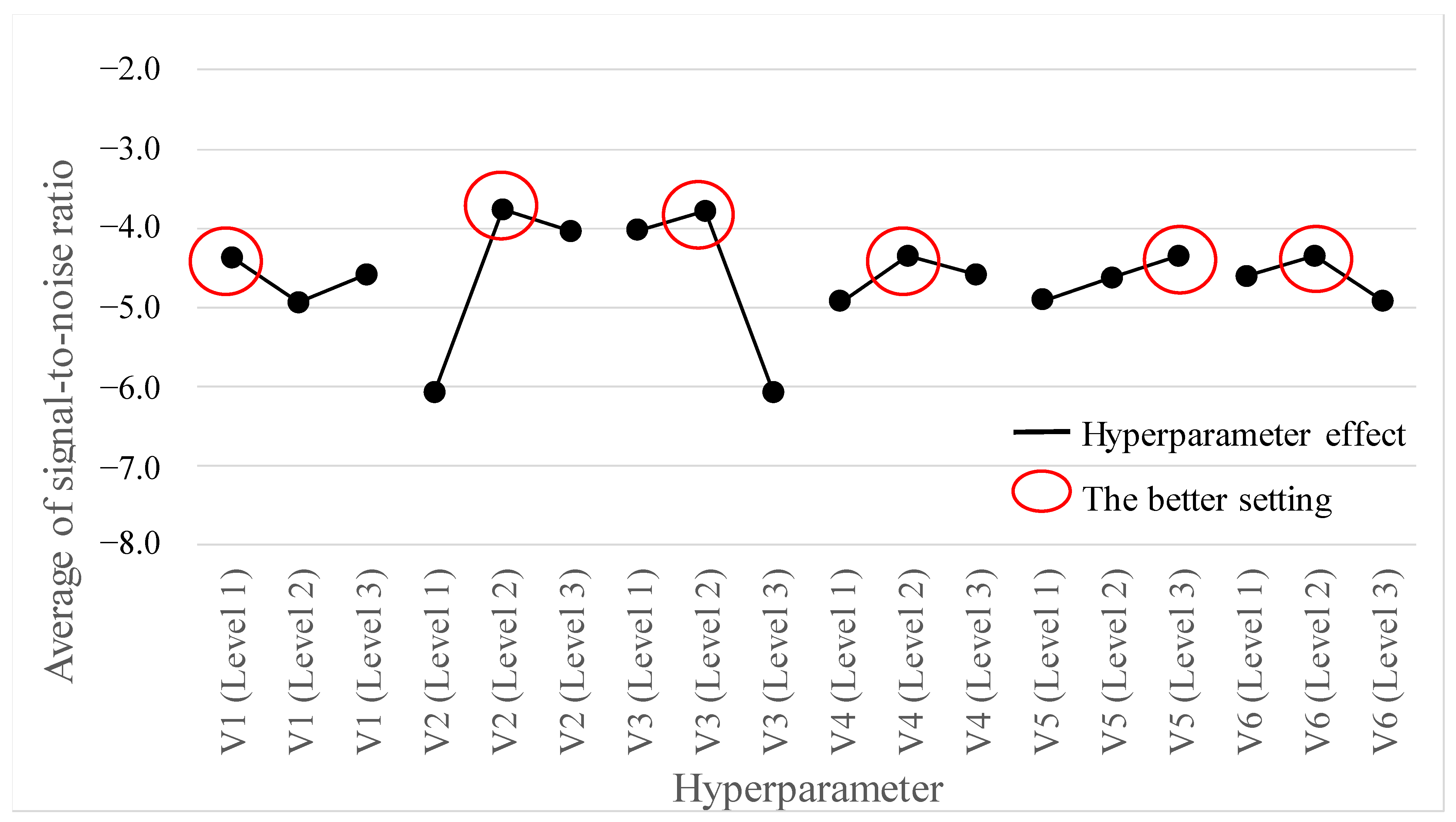
This study addressed the crucial challenge of improving prediction accuracy for cardiovascular disease (CVD). We proposed the TPTM-HANN-GA framework to fine-tune an ANN model for better CVD risk assessment. This method also revealed the relative impact of each hyperparameter (V₂ > V₃ > V₆ > V₄ > V₅ > V₁), guiding further optimization. Our analysis led to these optimal hyperparameter settings for the ANN model: V₁ (HL) = 4, V₂ (AF) = tanh, V₃ (OP) = sgd, V₄ (LR) = 0.3, V₅ (MR) = 0.9, and V₆ (HN) = 8.

In the subsequent phase, we refined the three hyperparameters’ predicted accuracies using the Taguchi method L₉(3⁴). This method facilitated the identification of optimal configurations with fewer trials. We then added the Monte Carlo method with a normal distribution probabilistic model into the second-stage Taguchi method of TSTO to increase the number of modeling data points. By employing the Monte Carlo method, this study aimed to construct a hyperparameter artificial neural network (HANN) model using a larger and more diverse dataset, theoretically enhancing the overall performance of the given dataset.

Table 9 serves as the data source for the HANN model, with V₄ (LR), V₅ (MR), and V₆ (HN) acting as input variables for predicting cardiovascular accuracy. The model boasts a single hidden layer for efficient learning. An amount of 80% of the dataset fuels the training process, while the remaining 20% is reserved for testing. To identify the optimal hyperparameter combination, we employed a grid search, evaluating various learning rates, momentum rates, and hidden node configurations. After 1000 training iterations, the search yielded these winning settings: learning rate = 0.25, moment rate = 0.9, and hidden nodes = 7. This configuration translates to a 3-7-1 HANN model architecture chosen based on minimizing the root mean square error (RMSE) on the test dataset.

To identify the optimal configuration of input variables for the HANN model, we employed a genetic algorithm (GA), leveraging a population size of 25. This work prioritizes individuals within the population for reproduction based on their predicted accuracy. Individuals exhibiting superior predictive performance are assigned a higher probability of selection. Crossover and mutation rates were set at 0.9 and 0.05, respectively, balancing exploration and stability. After 500 iterations, the GA identified the ultimate hyperparameter configuration: V₄ (LR) = 0.23425849, V₅ (MR) = 0.75462782, and V₆ (HN) = 7. To validate these findings, we conducted confirmation experiments and achieved an average accuracy of 74.25%. This underscores the effectiveness of the GA-optimized HANN model.

The proposed TPTM-HANN-GA framework achieved a 0.11% higher accuracy in predicting cardiovascular disease risk compared to the leading TSTO-ANN model. This indicates its ability to correctly identify an additional 77 patients from the 70,000 data points in the Kaggle Cardiovascular Disease dataset. It highlights the potential to enhance patient survival rates. In addition, TPTM-HANN-GA can perform a continuous value search for each continuous variable. This method has a larger search space and is more general than the discrete search method of the TSTO-ANN model, which is more likely to find the optimal solution. The GA used in this paper performed eight-digit and single-digit searches for LR (learning rate), MR (moment rate), and HN (hidden nodes), respectively.

The TPTM-HANN-GA framework offers several advantages over traditional grid search methods, notably by substantially reducing computational demands while maintaining the ideal accuracy.

In this study, we applied the HANN method to the GA to search for optimal settings of continuous hyperparameters. In contrast to the TSTO method, which only allows for discrete parameter searches (e.g., learning rate choices limited to 0.2, 0.3, and 0.4), HANN-TPTM-GA enables the simultaneous use of discrete and continuous variables. For instance, the learning rate can be selected continuously within the range of 0.2 to 0.4. Theoretically, it allows for an infinite number of learning rate choices. In our study, the identified optimal learning rate was 0.23425849. Consequently, the expanded search range makes it easier to find optimal solutions compared to TSTO-ANN. In our research, the achieved accuracy of 74.25% surpasses the 74.14% accuracy obtained with TSTO-ANN.

In the initial phase of the Taguchi method, experiments for model training were performed using the Taguchi orthogonal array L₁₈(2¹ × 3⁷) involving 54 runs, which required a total computation time of 33.9 min on a personal computer, translating to an average of about 0.63 min per run. Comparatively, considering the traditional grid search involving 2187 runs, this study did not execute all runs but estimated that at 0.63 min per run, completing the full set of 2187 runs would likely demand around 1373.8 min. The initial-phase Taguchi method enables a reduction in computation time by approximately 40 times.

In the second phase of the Taguchi method, a traditional grid search with three levels for each hyperparameter, repeated three times, would necessitate 81 trials, taking approximately 50.9 min to complete. Conversely, employing the Taguchi orthogonal array L₉(3⁴) reduced the number of experiments to 27, with an approximate total time requirement of 16.9 min. The second-phase Taguchi method enables a reduction in computation time by approximately three times.

In the final step, we applied a genetic algorithm to identify optimal hyperparameter configurations for accurate CVD Risk Prediction. This involved testing a total of 25 initial populations over 500 iterations, resulting in 12,500 tests. In contrast, if a traditional grid search were employed, it would entail 10⁸ × 10⁸ × 10 = 10¹⁷ tests, leading to an impractical consumption of time resources.

Our approach significantly mitigates computational demands, rendering it well-suited for low-power computers and edge artificial intelligence (edge AI) devices, which can achieve the goal of point-of-care testing (POCT), providing individuals a way to take charge of their heart health.

While the identified hyperparameters are tailored to the specific dataset used, exploring the adaptability of TPTM-HANN-GA to other medical domains could reveal significant potential. Additionally, relying solely on a single dataset limits generalizability. Incorporating independent datasets from diverse healthcare organizations in future research can enhance the technique’s validity. Furthermore, validating its efficacy with datasets from various sources will increase its credibility and generalizability.

In future work, the proposed TPTM-HANN-GA framework could be extended to address other deep learning-based medical image disease detection tasks, including pathological, CT, and X-ray images. The TPTM-HANN-GA framework is particularly suitable for application in clinical edge AI devices, which will provide more efficient training and accurate inference results for medical image disease detection tasks with limited computing resources.

5. Conclusions

This study proposes a novel TPTM-HANN-GA framework to improve the prediction of CVD risk. Compared with traditional grid search methods, TPTM-HANN-GA significantly enhances the prediction accuracy of an ANN model while minimizing computational costs, making it efficient and resource-friendly. TPTM-HANN-GA adapts to various neural networks, offering flexibility for implementation. The network architecture will be simplified and lightweight by incorporating optimal hyperparameter settings. These improvements enable the resulting ANN model to run efficiently on low-power computers, which offers individuals direct access to personalized CVD risk prediction, allowing them to effectively manage their heart health and accomplish the objective of point-of-care testing.

References

1. Martin, S.S.; Aday, A.W.; Almarzooq, Z.I.; Anderson, C.A.; Arora, P.; Avery, C.L.; Baker-Smith, C.M.; Gibbs, B.B.; Beaton, A.Z.; Boehme, A.K.; et al. 2024 Heart Disease and Stroke Statistics: A Report of US and Global Data From the American Heart Association. Circulation 2024, 149, e347–e913. [Google Scholar] [CrossRef]
2. Zhang, L.; Lu, H.; Yang, C. Global, regional, and national burden of stroke from 1990 to 2019: A temporal trend analysis based on the Global Burden of Disease Study 2019. Int. J. Stroke 2024. [Google Scholar] [CrossRef] [PubMed]
3. Gaziano, T.; Reddy, K.S.; Paccaud, F.; Horton, S.; Chaturvedi, V. Cardiovascular disease. In Disease Control Priorities in Developing Countries, 2nd ed.; Oxford University Press: New York, NY, USA, 2006. [Google Scholar]
4. Patnode, C.D.; Redmond, N.; Iacocca, M.O.; Henninger, M. Behavioral Counseling Interventions to Promote a Healthy Diet and Physical Activity for Cardiovascular Disease Prevention in Adults without Known Cardiovascular Disease Risk Factors: Up-dated evidence report and systematic review for the us preventive services task force. JAMA 2022, 328, 375–388. [Google Scholar] [CrossRef] [PubMed]
5. Tektonidou, M.G. Cardiovascular disease risk in antiphospholipid syndrome: Thrombo-inflammation and atherothrombosis. J. Autoimmun. 2022, 128, 102813. [Google Scholar] [CrossRef]
6. World Health Organization. The World Health Report: 2000: Health Systems: Improving Performance; World Health Organization: Geneva, Switzerland, 2000. [Google Scholar]
7. Said, M.A.; van de Vegte, Y.J.; Zafar, M.M.; van der Ende, M.Y.; Raja, G.K.; Verweij, N.; van der Harst, P. Contributions of Interactions Between Lifestyle and Genetics on Coronary Artery Disease Risk. Curr. Cardiol. Rep. 2019, 21, 89. [Google Scholar] [CrossRef] [PubMed]
8. Arpaia, P.; Cataldo, A.; Criscuolo, S.; De Benedetto, E.; Masciullo, A.; Schiavoni, R. Assessment and Scientific Progresses in the Analysis of Olfactory Evoked Potentials. Bioengineering 2022, 9, 252. [Google Scholar] [CrossRef] [PubMed]
9. Rahman, H.; Bukht, T.F.N.; Imran, A.; Tariq, J.; Tu, S.; Alzahrani, A. A Deep Learning Approach for Liver and Tumor Segmentation in CT Images Using ResUNet. Bioengineering 2022, 9, 368. [Google Scholar] [CrossRef] [PubMed]
10. Centracchio, J.; Andreozzi, E.; Esposito, D.; Gargiulo, G.D. Respiratory-Induced Amplitude Modulation of Forcecardiography Signals. Bioengineering 2022, 9, 444. [Google Scholar] [CrossRef] [PubMed]
11. Ullah, M.; Hamayun, S.; Wahab, A.; Khan, S.U.; Rehman, M.U.; Haq, Z.U.; Rehman, K.U.; Ullah, A.; Mehreen, A.; Awan, U.A.; et al. Smart technologies used as smart tools in the management of cardiovascular disease and their future perspective. Curr. Probl. Cardiol. 2023, 48, 101922. [Google Scholar] [CrossRef] [PubMed]
12. Dritsas, E.; Trigka, M. Efficient data-driven machine learning models for cardiovascular diseases risk prediction. Sensors 2023, 23, 1161. [Google Scholar] [CrossRef] [PubMed]
13. Yashudas, A.; Gupta, D.; Prashant, G.C.; Dua, A.; AlQahtani, D.; Reddy, A.S.K. DEEP-CARDIO: Recommendation System for Cardiovascular Disease Prediction using IOT Network. IEEE Sens. J. 2024. [Google Scholar] [CrossRef]
14. Subramani, S.; Varshney, N.; Anand, M.V.; Soudagar, M.E.M.; Al-Keridis, L.A.; Upadhyay, T.K.; Alshammari, N.; Saeed, M.; Subramanian, K.; Anbarasu, K.; et al. Cardiovascular diseases prediction by machine learning incorporation with deep learning. Front. Med. 2023, 10, 1150933. [Google Scholar] [CrossRef] [PubMed]
15. Yang, L.; Peavey, M.; Kaskar, K.; Chappell, N.; Zhu, L.; Devlin, D.; Valdes, C.; Schutt, A.; Woodard, T.; Zarutskie, P.; et al. Development of a dynamic machine learning algorithm to predict clinical pregnancy and live birth rate with embryo morphokinetics. F&S Rep. 2022, 3, 116–123. [Google Scholar] [CrossRef] [PubMed]
16. Smith, B.R.; Edelman, E.R. Nanomedicines for cardiovascular disease. Nat. Cardiovasc. Res. 2023, 2, 351–367. [Google Scholar] [CrossRef]
17. Wijemunige, N.; Rannan-Eliya, R.P.; van Baal, P.; O’donnell, O. Optimizing cardiovascular disease risk screening in a low-resource setting: Cost-effectiveness of program modifications in Sri Lanka modelled with nationally representative survey data. BMC Public Health 2023, 23, 1792. [Google Scholar] [CrossRef] [PubMed]
18. Olisah, C.C.; Smith, L.; Smith, M. Diabetes mellitus prediction and diagnosis from a data preprocessing and machine learning perspective. Comput. Methods Programs Biomed. 2022, 220, 106773. [Google Scholar] [CrossRef] [PubMed]
19. Luengo-Fernandez, R.; Walli-Attaei, M.; Gray, A.; Torbica, A.; Maggioni, A.P.; Huculeci, R.; Bairami, F.; Aboyans, V.; Timmis, A.D.; Vardas, P.; et al. Economic burden of cardiovascular diseases in the European Union: A population-based cost study. Eur. Hear. J. 2023, 44, 4752–4767. [Google Scholar] [CrossRef]
20. Čáp, J.; Miertová, M.; Bóriková, I.; Žiaková, K.; Tomagová, M.; Gurková, E. Trust in healthcare professionals of people with chronic cardiovascular disease. Nurs. Ethics 2023. [Google Scholar] [CrossRef] [PubMed]
21. Arroyo, J.C.T.; Delima, A.J.P. An Optimized Neural Network Using Genetic Algorithm for Cardiovascular Disease Prediction. J. Adv. Inf. Technol. 2022, 13, 95–99. [Google Scholar] [CrossRef]
22. Kim, M.-J. Building a Cardiovascular Disease Prediction Model for Smartwatch Users Using Machine Learning: Based on the Korea National Health and Nutrition Examination Survey. Biosensors 2021, 11, 228. [Google Scholar] [CrossRef]
23. Khan, A.; Qureshi, M.; Daniyal, M.; Tawiah, K. A Novel Study on Machine Learning Algorithm-Based Cardiovascular Disease Prediction. Health Soc. Care Community 2023, 2023, 1406060. [Google Scholar] [CrossRef]
24. Moon, J.; Posada-Quintero, H.F.; Chon, K.H. A literature embedding model for cardiovascular disease prediction using risk factors, symptoms, and genotype information. Expert Syst. Appl. 2023, 213, 118930. [Google Scholar] [CrossRef]
25. Rosenblatt, F. Principles of Neurodynamics: Perceptrons and the Theory of Brain Mechanisms; Spartan Books: New York, NY, USA, 1962. [Google Scholar]
26. Olden, J.D.; Jackson, D.A. Illuminating the “black box”: A randomization approach for understanding variable contributions in artificial neural networks. Ecol. Model. 2002, 154, 135–150. [Google Scholar] [CrossRef]
27. Stern, H.S. Neural Networks in Applied Statistics. Technometrics 1996, 38, 205–214. [Google Scholar] [CrossRef]
28. McClelland, J.L.; Rumelhart, D.E. Explorations in Parallel Distributed Processing: A Handbook of Models, Programs, and Exercises, 1st ed.; MIT Press: London, UK, 1989. [Google Scholar]
29. Fausett, L. Fundamentals of Neural Networks: An Architecture, Algorithms, and Applications; Prentice Hall: New Jersey, NJ, USA, 1994. [Google Scholar]
30. Hagan, M.T.; Demuth, H.B.; Beale, M. Neural Network Design; PWS: Boston, MA, USA, 1995. [Google Scholar]
31. Katona, T.; Tóth, G.; Petró, M.; Harangi, B. Developing New Fully Connected Layers for Convolutional Neural Networks with Hyperparameter Optimization for Improved Multi-Label Image Classification. Mathematics 2024, 12, 806. [Google Scholar] [CrossRef]
32. Franchini, G. GreenNAS: A Green Approach to the Hyperparameters Tuning in Deep Learning. Mathematics 2024, 12, 850. [Google Scholar] [CrossRef]
33. Malhotra, P.; Gupta, S.; Koundal, D.; Zaguia, A.; Enbeyle, W. Deep Neural Networks for Medical Image Segmentation. J. Health Eng. 2022, 2022, 9580991. [Google Scholar] [CrossRef] [PubMed]
34. You, Y.-S.; Lin, Y.-S. A Novel Two-Stage Induced Deep Learning System for Classifying Similar Drugs with Diverse Packaging. Sensors 2023, 23, 7275. [Google Scholar] [CrossRef] [PubMed]
35. Pantic, I.; Paunovic, J.; Cumic, J.; Valjarevic, S.; Petroianu, G.A.; Corridon, P.R. Artificial neural networks in contemporary toxicology research. Chem. Interact. 2022, 369, 110269. [Google Scholar] [CrossRef] [PubMed]
36. Lin, Y.-S.; Huang, P.-H.; Chen, Y.-Y. Deep Learning-Based Hepatocellular Carcinoma Histopathology Image Classification: Accuracy Versus Training Dataset Size. IEEE Access 2021, 9, 33144–33157. [Google Scholar] [CrossRef]
37. He, B.; Hu, W.; Zhang, K.; Yuan, S.; Han, X.; Su, C.; Zhao, J.; Wang, G.; Wang, G.; Zhang, L. Image segmentation algorithm of lung cancer based on neural network model. Expert Syst. 2022, 39, e12822. [Google Scholar] [CrossRef]
38. Poradzka, A.A.; Czupryniak, L. The use of the artificial neural network for three-month prognosis in diabetic foot syndrome. J. Diabetes Its Complicat. 2023, 37, 108392. [Google Scholar] [CrossRef] [PubMed]
39. Krasteva, V.; Christov, I.; Naydenov, S.; Stoyanov, T.; Jekova, I. Application of Dense Neural Networks for Detection of Atrial Fibrillation and Ranking of Augmented ECG Feature Set. Sensors 2023, 21, 6848. [Google Scholar] [CrossRef] [PubMed]
40. Su, C.T. Quality Engineering: Off-Line Methods and Applications, 1st ed.; CRC Press: Boca Raton, FL, USA, 2013. [Google Scholar]
41. Parr, W.C. Introduction to Quality Engineering: Designing Quality into Products and Processes; Asia Productivity Organization: Tokyo, Japan, 1986. [Google Scholar]
42. Taguchi, G.; Elsayed, E.A.; Hsiang, T.C. Quality Engineering in Production Systems; McGraw-Hill: New York, NY, USA, 1989. [Google Scholar]
43. Ross, P.J. Taguchi Techniques for Quality Engineering: Loss Function, Orthogonal Experiments, Parameter and Tolerance Design, 2nd ed.; McGraw-Hill: New York, NY, USA, 1996. [Google Scholar]
44. Kaziz, S.; Ben Romdhane, I.; Echouchene, F.; Gazzah, M.H. Numerical simulation and optimization of AC electrothermal microfluidic biosensor for COVID-19 detection through Taguchi method and artificial network. Eur. Phys. J. Plus 2023, 138, 96. [Google Scholar] [CrossRef] [PubMed]
45. Tseng, H.-C.; Lin, H.-C.; Tsai, Y.-C.; Lin, C.-H.; Changlai, S.-P.; Lee, Y.-C.; Chen, C.-Y. Applying Taguchi Methodology to Optimize the Brain Image Quality of 128-Sliced CT: A Feasibility Study. Appl. Sci. 2022, 12, 4378. [Google Scholar] [CrossRef]
46. Karimipourfard, M.; Sina, S.; Mahani, H.; Karimkhani, S.; Sadeghi, M.; Alavi, M.; Faghihi, R. A Taguchi-optimized Pix2pix generative adversarial network for internal dosimetry in 18F-FDG PET/CT. Radiat. Phys. Chem. 2024, 218, 111532. [Google Scholar] [CrossRef]
47. Bayraktar, A.; Gürsoy, C. Production of New Nano-Bacterial Cellulose with Lactobacillus rhamnosus by Using Whey Waste as Substrate with Optimization Taguchi Method, which has the potential to be used in many biomedical products. Res. Sq. 2024. [Google Scholar] [CrossRef]
48. Goldberg, D.E. Genetic Algorithm in Search, Optimization and Machine Learning, 1st ed.; Addison-Wesley: New York, NY, USA, 1989. [Google Scholar]
49. Renders, J.-M.; Flasse, S. Hybrid methods using genetic algorithms for global optimization. IEEE Trans. Syst. Man Cybern. Part B (Cybern.) 1996, 26, 243–258. [Google Scholar] [CrossRef] [PubMed]
50. Neumann, A.; Hajji, A.; Rekik, M.; Pellerin, R. Genetic algorithms for planning and scheduling engineer-to-order production: A systematic review. Int. J. Prod. Res. 2023, 62, 2888–2917. [Google Scholar] [CrossRef]
51. Altarabichi, M.G.; Nowaczyk, S.; Pashami, S.; Mashhadi, P.S. Fast Genetic Algorithm for feature selection—A qualitative approximation approach. In Proceedings of the Companion Conference on Genetic and Evolutionary Computation, Lisbon, Portugal, 15–19 July 2023; pp. 11–12. [Google Scholar] [CrossRef]
52. Aziz, R.M.; Mahto, R.; Goel, K.; Das, A.; Kumar, P.; Saxena, A. Modified genetic algorithm with deep learning for fraud transactions of ethereum smart contract. Appl. Sci. 2023, 13, 697. [Google Scholar] [CrossRef]
53. Ghezelbash, R.; Maghsoudi, A.; Shamekhi, M.; Pradhan, B.; Daviran, M. Genetic algorithm to optimize the SVM and K-means algorithms for mapping of mineral prospectivity. Neural Comput. Appl. 2023, 35, 719–733. [Google Scholar] [CrossRef]
54. Ulianova, S. Cardiovascular Disease Dataset. 2019. Available online: https://www.kaggle.com/datasets/sulianova/cardiovascular-disease-dataset (accessed on 17 February 2023).
55. Lin, C.-M.; Lin, Y.-S. Utilizing a Two-Stage Taguchi Method and Artificial Neural Network for the Precise Forecasting of Cardiovascular Disease Risk. Bioengineering 2023, 10, 1286. [Google Scholar] [CrossRef] [PubMed]
56. Kroese, D.P.; Brereton, T.; Taimre, T.; Botev, Z.I. Why the Monte Carlo method is so important today. Wiley Interdiscip. Rev. Comput. Stat. 2014, 6, 386–392. [Google Scholar] [CrossRef]
Figure 1. Proposed method. The proposed method integrates the two-phase Taguchi method (TPTM), hyperparameter artificial neural network (HANN), and genetic algorithm (GA) to optimize hyperparameters for an ANN model used in predicting CVD risk.
Mathematics 12 01303 g001
Figure 2. Chart of hyperparameter response for the average of SN ratio in L18(21 × 37) array. In this chart, we can find the higher SN ratios for each hyperparameter.
Mathematics 12 01303 g002
Figure 3. 11-8-8-8-8-1 architecture for ANN model of cardiovascular disease.
Mathematics 12 01303 g003
Figure 4. 3-7-1 architecture of the HANN model. The HANN model used learning rate (V4), momentum rate (V5), and hidden nodes (V6) as input variables to predict cardiovascular disease accuracy.
Mathematics 12 01303 g004
Figure 5. 11-7-7-7-7-1 architecture for ANN model of cardiovascular disease.
Mathematics 12 01303 g005